

NBER WORKING PAPER SERIES
HOW THE SUBPRIME CRISIS WENT GLOBAL:EVIDENCE FROM BANK CREDIT DEFAULT SWAP SPREADS
Barry EichengreenAshoka Mody
Milan NedeljkovicLucio Sarno
Working Paper 14904http://www.nber.org/papers/w14904
NATIONAL BUREAU OF ECONOMIC RESEARCH1050 Massachusetts Avenue
Cambridge, MA 02138April 2009
The authors are respectively with the University of California, Berkeley; the International MonetaryFund; the University of Warwick; and the Cass Business School and the Centre for Economic PolicyResearch. They are grateful to Charlie Kramer for comments and to Susan Becker and Anastasia Guscinafor valuable research assistance. The views expressed here are those of the authors and should notbe attributed to the International Monetary Fund, its management, its Executive Directors, or the NationalBureau of Economic Research.
NBER working papers are circulated for discussion and comment purposes. They have not been peer-reviewed or been subject to the review by the NBER Board of Directors that accompanies officialNBER publications.
© 2009 by Barry Eichengreen, Ashoka Mody, Milan Nedeljkovic, and Lucio Sarno. All rights reserved.Short sections of text, not to exceed two paragraphs, may be quoted without explicit permission providedthat full credit, including © notice, is given to the source.

How the Subprime Crisis Went Global: Evidence from Bank Credit Default Swap SpreadsBarry Eichengreen, Ashoka Mody, Milan Nedeljkovic, and Lucio SarnoNBER Working Paper No. 14904April 2009JEL No. F36,G15,G18
ABSTRACT
How did the Subprime Crisis, a problem in a small corner of U.S. financial markets, affect the entireglobal banking system? To shed light on this question we use principal components analysis to identifycommon factors in the movement of banks' credit default swap spreads. We find that fortunes of international banks rise and fall together even in normal times along with short-term global economicprospects. But the importance of common factors rose steadily to exceptional levels from the outbreakof the Subprime Crisis to past the rescue of Bear Stearns, reflecting a diffuse sense that funding andcredit risk was increasing. Following the failure of Lehman Brothers, the interdependencies brieflyincreased to a new high, before they fell back to the pre-Lehman elevated levels – but now they moreclearly reflected heightened funding and counterparty risk. After Lehman's failure, the prospect ofglobal recession became imminent, auguring the further deterioration of banks' loan portfolios. Atthis point the entire global financial system had become infected.
Barry EichengreenDepartment of EconomicsUniversity of California, Berkeley549 Evans Hall 3880Berkeley, CA 94720-3880and [email protected]
Ashoka ModyResearch DepartmentInternational Monetary Fund700 19th Street, NWWashington, DC [email protected]
Milan NedeljkovicDepartment of EconomicsThe University of WarwickGibbet Hill RoadCoventry, CV4 7AL, [email protected]
Lucio SarnoCass Business School106 Bunhill RowLondon, EC1Y 8TZ, UKUnited [email protected]
2
I. INTRODUCTION
One enduring question about the financial turbulence that engulfed the world starting
in the summer of 2007 is how problems in a small corner of U.S. financial markets—
securities backed by subprime mortgages accounting for only some 3 per cent of U.S.
financial assets—could infect the entire U.S. and global banking systems. This paper seeks to
shed further light on that question. We analyze the risk premium on debt owed by individual
banks as measured by banks’ credit default swap (CDS) spreads, focusing on the CDS
spreads of the 45 largest financial institutions in the United States, the United Kingdom,
Germany, Switzerland, France, Italy, Netherlands, Spain and Portugal.2
We use principal components analysis to extract the common factors underlying
weekly variations in the CDS spreads of individual banks. If the spreads for different banks
move independently, then we can infer that the risk of bank failure is driven by bank-specific
factors. If they move together then we infer that banks are perceived as subject to common
risks. This provides us with the first bit of evidence on how the crisis spread.
In addition to estimating the importance of common factors we attempt to ascertain
what they reflect. We examine the correlation between the common factors on the one hand
and real-economy influences outside the financial system, transactional relationships among
2 These swaps are insurance contracts. The buyer of the CDS makes payments to the seller in order to receive a payment if a credit instrument (e.g. a bond or a loan) goes into default or in the event of a specified credit event, such as bankruptcy. The spreads are, in effect, a measure of the credit risk or the insurance premium charged. Although CDS spreads are implicitly spreads on the issuers’ bonds, they have the advantage, as Longstaff et al. (2008) point out, that they are “less encumbered by covenants and guarantees.” However, there has been a recent concern that speculative pressure within the CDS market sometimes causes the swaps to become delinked from their function of hedging against default (Soros, 2009). Longstaff et al. (2008) analyze spreads on sovereign CDS, whereas Zhang, Zhou, and Zhu (2008) examine the determinants of spreads on corporate CDS spreads.

3
banks, and transactional influences between banks and other parts of the financial system on
the other.3
We reach three conclusions. First, the share of common factors was already quite
high, at 62 percent, prior to the outbreak of the Subprime Crisis in July 2007. Banks’
fortunes rose and fell together to a considerable extent, in other words, even before the crisis.
These common factors were correlated with U.S. high-yield spreads—the premium paid
relative to Treasury bonds by U.S. corporations that had less than investment grade credit
ratings—which we take as an indicator of the perceived probability of default by less
creditworthy U.S. corporations, which in turn reflects economic growth prospects.4 For
obvious reasons, those defaults and the growth performance that drives them have major
implications for the condition of the banking system even in normal times.
The share of the variance accounted for by common factors then rose to 77 percent in
the period between the July 2007 eruption of the Subprime Crisis and Lehman’s failure in
September 2008. This is indicative of a perception that banks as a class faced higher
common risks than before. At the same time, the correlation between the common factors
and U.S. high-yield spreads declined, while the correlation with measures of banks’ own
credit risk and of generalized risk aversion increased (Brunnermeier, 2009). An
interpretation is that the Subprime Crisis made investors more wary about the risks in bank
3 To be clear, we do not attempt to identify causality. However, the correlations offer a rich set of stylized characterizations. These characterizations are likely to be the basis for defining and probing more subtle hypotheses. 4 These high-yield spreads have been found to be good predictors of U.S. growth at horizons of about a year, reflecting a financial-accelerator interaction between credit markets and the real economy (Mody and Taylor, 2003). Because European high-yield spreads are closely correlated with US spreads and, as such, offer no additional information, U.S. high-yield spreads (spreads of corporations with less than investment-grade rating) are also a measure of global prospects.
4
portfolios for reasons largely independent of the evolution of the real economy but that lack
of detailed information on those risks led them to treat all banks as riskier rather than
discriminating among them.
Following Lehman’s failure, there was a further brief increase in the share of the
variance accounted for by the common components. Then, although the level of CDS spreads
remained high, the share of their variation accounted for by the common component fell back
relatively quickly to levels about those that prevailed just before the Lehman episode. In
other words, the common movements declined from their peaks but remained at the post-
Bear Stearns elevated levels. Thus, the perception persisted that the banks’ fortunes were
linked. The correlation between the common factors and high-yield corporate spreads also
reemerged, evidently reflecting the perception that a global recession was now in train. More
importantly, the common component of CDS spreads became more highly correlated with
measures of funding and credit risk as measured by spreads in the asset-backed commercial
paper market and LIBOR minus the overnight index swap. An interpretation is that whereas
in the July 2007-September 2008 period investors became more aware of systemic risk in an
unfocused sense, Lehman’s failure caused that common risk to be more concretely identified
with both developments in the real economy and specific problems in the financial system.
In sum, then, our answer to the question posed in the title is thus as follows. Banks
fortunes rise and fall together even in normal times. But the importance of common factors
rose to exceptional levels between the outbreak of the Subprime Crisis and the rescue of Bear
Stearns, reflecting increased diffuse sense that credit risk was increasing. The period
following the failure of Lehman Brothers then saw a further increase in those
interdependencies, reflecting heightened funding and counterparty risk. In addition there
5
were direct spillovers, as opposed to common movements, from the CDS spreads of U.S.
banks to those of European banks. After Lehman’s failure the prospect of global recession
became imminent, auguring the further deterioration of banks’ loan portfolios. At this point
the entire global financial system had become infected.
It is helpful to be clear about what this paper does not do. It does not pinpoint any one
bank or set of banks as systemically-important. Rather, the extent of comovement in spreads
points to tendencies of the degree to which the system is perceived to be tied to common
factors. An individual bank within the set examined may be more or less tied to the common
factors to the extent that it has a large or small extent of idiosyncratic risk. Ultimately, then,
the methodology outlined here is a guide for policy only to the extent that it highlights
overall trends. The task of determining the systemic importance of an individual bank
requires examining the data in the books of the banks—or worse, at data that should be on
the books but is not.
The rest of the paper is organized as follows. Section II specifies a dynamic factor
model in which common latent factors explain the movement of the CDS spreads of the 45
banks in our sample. The model is estimated using principal components analysis, allowing
the contributions of the components to change over time. In Section III, we consider the
possibility of additional spillovers from inter-bank exposures that go beyond the common
movements identified by the latent factors. Then in Section IV, we describe the changing
correlations between these latent factors and a number of high frequency financial series. A
final section concludes.
6
II. COMMON FACTORS IN CDS SPREADS
We start by decomposing the movement in credit default swap (CDS) spreads of 45
global banks into common and idiosyncratic components.5 The sample runs from July 29,
2002 to November 28, 2008.6 The data are 5-year CDS spreads, the five year maturity being
the most widely traded. We use end-of-day quotes from the New York market for payment in
U.S. dollars based on U.S. dollar-denominated notional amounts. As is customary, the
spreads are denominated in basis points (100 basis points equal 1 percentage point). These
are averaged over the week to obtain a weekly series, smoothing out sharp daily movements
and irregular trading, yielding 331 observations per bank. The data are from Bloomberg.
II.1 Preliminary data analysis
Table 1 reports summary statistics on spreads for 45 banks. Average spreads over the
period vary significantly across banks (from a low of 17 for Rabobank to a high of 101 basis
points for AIG).7 Our interest is not so much in the cross-sectional variation at this stage,
however, as in the variation over time, which has been substantial. Unlike sovereign CDS
spreads where the standard deviations are typically smaller than the means, the standard
deviations of the CDS spreads of financial institutions studied here are close to the means
and sometimes larger. The minimum/maximum values further highlight the considerable
5 The term “banks” is used throughout, although some insurance companies are also included in the sample.
6 Thereafter, the intense involvement of the U.S. authorities in managing the short-term vulnerability of the financial sector increasingly reflects the official interventions, which, because they operated differentially across the institutions, limits the validity of a market-driven common set of influences on their CDS.
7 This variation is, however, smaller than the 100-fold variation in premia across the Japanese and Brazilian sovereigns in the sample analyzed by Longstaff et al. (2008).
7
time-series variation. For example, the spread for Merrill Lynch ranges from 15 to 473 basis
points; in Europe, the range for Commerzbank varies from 8 to 260 basis points.
Figure 1 tracks the time variation in median spreads for all banks, U.S. banks, and
European banks. In 2002, after the tech bubble burst and confidence was challenged by the
events of September 11, 2001, CDS spreads were elevated. Some banks were able to
purchase protection at relatively low spreads of 20-50 basis points, but others paid more than
100 basis points. Subsequently spreads declined everywhere. The low point was the week of
January 17, 2007 when the median spread in the full sample of 45 banks was 7.5 basis points.
Thereafter, spreads increased gradually, reaching a median of 12 basis points in the second
week of July 2007. But even in that week, the highest spread was 55 basis points for Bear
Stearns.8 In contrast, the subsequent rise in spreads was dramatic with twin peaks
corresponding to the Bear Stearns rescue and the Lehman Brothers failure. For U.S. banks, a
high of 417 basis points was reached following the severe stress after the Lehman failure
during the week of October 1, 2008; the median spread then moderated to 268 basis points in
the last week of November 2008. The corresponding numbers for the European banks were
130 and 97 basis points, respectively.
II.2 A dynamic factor model of CDS spreads
The first question we ask is whether the movements in spreads reflected common
drivers. To answer that question we estimate the “latent” or unobserved factors generating
common movements. The relationship between these unobserved factors ( tF ) and the
8 Someone, evidently, new about the extent of its leverage.
8
observed spreads ( tiX , ) can be approximately represented by a dynamic factor model
(Chamberlain and Rothchild, 1983):
ittiithiti XLFX εφ ++Λ= −1,,, )( (1)
tiX , is a vector of the weekly changes in CDS spreads of each of the 45 banks, where “i”
refers to a bank and “t” is the time subscript. iΛ is a matrix of factor loadings, and thF , are
latent factors (h=1,…,k). The estimation procedure allows for tiX , to be serially correlated
and for itε to be cross-sectionally correlated and heteroscedastic.9 Stacking the terms,
specification (1) can be equally represented as:
ε+Φ+Λ′= XLFX )( (2)
where X and ε are TxN matrices, F is a Txk, and Λ is a Nxk matrix.
The idea here is that the covariance among the series can be captured by a few
unobserved common factors. The latent factors and their loadings can be consistently
estimated by the method of principal components. As Bai and Ng (2002, 2008) and Stock
and Watson (2002) show, the principal component (PC) estimator enables us to identify
factors up to a change of sign and consistently estimate them up to an orthonormal
transformation.10 The procedure also provides a measure of the fraction of the total variation
explained by each factor, which is computed as the ratio between the k largest eigenvalues of
the matrix X′X divided by the sum of all eigenvalues.
9 Note, however, that the contribution of the idiosyncratic covariances to the total variance needs to be bounded (Bai and Ng, 2008), which puts a limit on the amount of cross-correlation and heteroscedasticity.
10 Note that the consistency is related to the space spanned by the factors and not with respect to the individual factor estimates. Under standard regulatory conditions, Bai and Ng (2008) establish consistency of the estimates of the factor space provided that T/N²→0, which holds in our case.
9
The data for each bank are first filtered for autocorrelation since in the presence of
serial correlation the covariance matrix of the data will not have the factor structure (exact or
approximate) and as such can lead to biased inference. To assess the changes over time, the
model is estimated recursively after the first 150 data points: as such, the filtering is also
performed recursively. At each recursion an AR(p) model is applied to each series, where the
order, p, is determined using the individual partial autocorrelation function (PACF) and
residuals from the AR(p) model are used as the filtered series. The data is then tested for non-
stationarity and, as expected, unit root tests indicate no evidence of nonstationarity in the
series.11 Finally, all series are standardized at each recursion since principal component
estimates are not scale invariant.
II.3 Estimation results and discussion
Figure 2 shows changes over time in the contributions of the common factors to the
total variance in the CDS data. Recall that up until mid-July 2007, i.e., before the start of the
subprime crisis, absolute movements in bank CDS spreads were small. The principal
components analysis shows that even in this relatively tranquil period the perceived riskiness
of different international banks moved together to a considerable extent. The first component
contributed just above 40 percent of these movements and the second a further 10 percent.
Together the first four common factors explained about 60 percent of movements in CDS
spreads in this period.12 The statistical procedure does not tell us of course whether these
11 To save space, these results are not reported.
12 Factors other than the first four individually explained less than 4 percent of the variation. Thus, our analysis below focuses on the PC estimates obtained using the four factor “space.” This is supported by the results obtained by running the Onatski’s (2006) criterion for determination of the number of factors in the data
(continued)
10
common influences reflected interconnections within the banking system or were the result
of common external factors. To explore that distinction, in Section IV, we report evidence on
the correlations of the common “unobserved” factors and observed variables representing
real economic prospects and metrics of banks’ funding stress and their systemic credit risk.
A new phase commenced in July 2007, when HSBC announced large subprime-mortgage
related losses and CDS spreads rose sharply. While spreads retreated somewhat in the
months thereafter, they remained at significantly higher levels. Nevertheless, July 2007 saw
the start of a tendency towards an increase in the comovement of spreads. The rise in the
share of variance explained by the first factor and the first four factors combined trended up
even as the average spreads rose and fell. Thus, while the sense of crisis went into remission
periodically in late 2007 and early 2008, the perception remained that banks faced common
risks. By early March 2008, prior to the rescue of Bear Stearns, the share of the first
component had risen by about 15 percentage points to 56 percent.
The importance of the common factors continued to increase following the Bear
Stearns rescue, reaching a new high in May 2008, at which point the first common factor
explained almost 60 percent of the variance of CDS spreads. Then, the period between May
and September 2008 was one of general weakness of financial-market indicators. The share
of the variance explained by common components of CDS spreads exhibited some slight
tendency to decline in this period, although it remained not very far below the high level
reached in May.
through a grid of parameter values. The Bai and Ng (2002) information criterion does lead to the possibility of more than four factors, but this criterion tends to overestimate the number of factors in samples with relatively small cross-sections and high cross-correlations (Anderson and Vahid, 2007, Onatski, 2006). As a practical matter, our results remain the same with either 3 or 5 factors.
11
The failure of Lehman Brothers was accompanied by a further increase in
comovement of spreads.13 The share of the variation accounted for by the first principal
component jumped to 65 percent, while the share accounted for by the first four reached 80
percent. However, there was moderation of the comovement by the first week of October, as
the share of the variance accounted for by the common factors fell back to pre-Lehman
levels.
To get a sense of whether the degree of commonality we observe for international
banks is high or low, we can compare these results with those of Longstaff et al. (2008) for
sovereign CDS spreads. Longstaff et al. found that the fraction of the variance of spreads on
the CDS of 26 sovereigns explained by the first component varied between 32 and 48
percent. Note that they used monthly (rather than weekly) changes in spreads and the higher
share is for months in which observations were available for all sovereigns. These features of
their analysis smooth out some part of the idiosyncratic movements and, to that extent, might
overstate the commonality. As such, the initial—pre-subprime—contribution of the first
component of banks’ spreads at about a 40 percent share is at least in a comparable range,
and possibly implies greater commonality. That share of the first component for the banks, as
we have reported, then rose to approximately 60 percent just before the Lehman failure and
further to 65 percent just after. When considering the first four components, Longstaff et al.
(2008) find that they explain 60 to 70 percent of the share of sovereign spreads variation,
which is comparable to our range of 60 to 80 percent. The implication also is that for
sovereign spreads, the second component and beyond have a more substantial contribution
13 As well as in the aggregate share of all four components.
12
than is the case for banks, implying greater variety of global common influences on
sovereign spreads.
III. ADDITIONAL SPILLOVERS
In this section, we investigate whether, once the common factors are considered, the
CDS spread of a particular bank is further influenced by current and lagged changes in CDS
spreads of other banks. In other words, we ask whether there is significant information in
CDS spreads of other banks over and above that contained in the common factors.
These spillover tests are performed by regressing the change in the (non-filtered) CDS spread
of a bank “i” on its own lags, the common factors, and the (lagged and current) changes in
CDS spreads of another bank (bank “j), as in equation (3). Since the CDS data exhibit a
break in the last week of July 2007 we also added a dummy variable for the sub-prime
period, where )(1, τ≥= − tIXD tjt :14
itttjjtiiihiti uDXLXLFX ++++Λ= −− δλφ 1,1,,, )()( (3)
Equation (3) was estimated for each pair of banks, which yielded a total of 2025 regressions.
In each case, we tested for the statistical significance of the coefficients jλ by computing the
heteroskedascity robust Lagrange multiplier (LM) test of specification (3).15 The restrictions
are tested using a standard χ² test.16
14 Bai and Ng (2006a) showed that the so-called “factor-augmented” regressions yield consistent estimates of the parameters as T,N→∞ provided that √T/N→0. Of course, in a finite sample the estimation error will not disappear completely.
15 The heteroscedasticity robust estimate of the covariance matrix was obtained using the Davidson and MacKinnon (1985)’s transformation of the squared residuals. 16 Simulation results in Clark and McCracken (2005) and Rossi (2005) establish that the likelihood ratio test (and other asymptotically equivalent tests) does not lose power to detect the significance of variables in OLS
(continued)
13
In only about 2½ percent of the 2025 possible relationships is the CDS spread of
another bank significant at the 5 percent significance level. This supports the validity of the
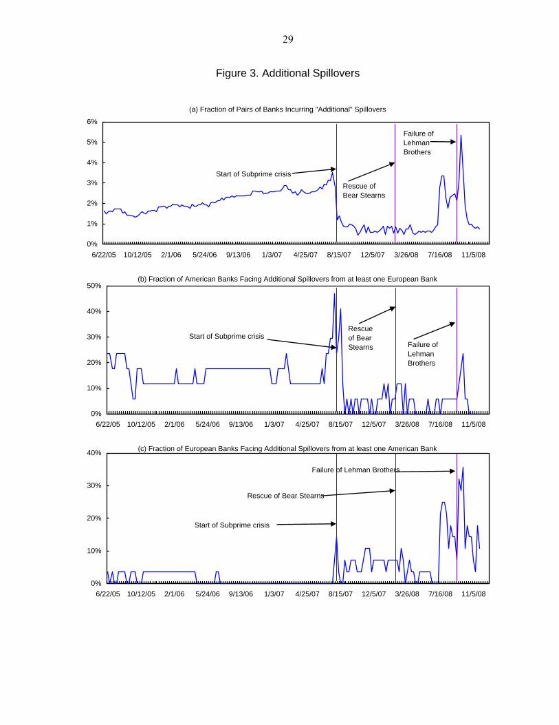
common factors estimated in the preceding section.17 The relatively few additional spillovers
we identify are illustrated in Figure 3(a). Following the start of the sub-prime crisis, the
incidence of such spillovers declined, implying that the commonality is well captured by the
latent factors. However, the additional spillovers increased notably starting in mid-July 2008
and reached their maximum during the Lehman Brothers crisis. An interpretation is that not
just global economic drivers (which are presumably being picked up by the common factors)
but also counterparty risk and other similarities in a few banks’ portfolios (which are being
captured by the additional spillovers) figured importantly in individual CDS spreads around
the time of the Lehman Brothers failure.18 The banks for which additional spillovers matter
tend to be well-known names: they include ING, Rabobank, Royal Bank of Scotland, and
UBS in Europe, and Bank of America, J.P. Morgan, and Morgan Stanley in the United
States.
Our procedure also allows us to glean some evidence of international spillovers. Here
we consider the percentage of banks in the U.S. significantly influenced by a bank in the
regression subject to the structural break provided that the relationship existed for any subsample (i.e. before or after the break). It is well known that in the presence of breaks and heteroscedasticity, all classical tests may be oversized (Hansen, 2000). We also run the robust bootstrap LM test based on the fixed design wild bootstrap (Hansen, 2000) and recursive wild bootstrap (Goncalves and Kilian, 2004), but the results were not significantly different. In addition, we also performed a battery of Monte Carlo experiments using the robust LM and Wald statistics (with and without bootstrapping) and while both tests had similar power properties the LM test had more conservative rejection rates. 17 In contrast, if we estimate the same specification without controlling for common factors, more than half of the relationships show (misleading) evidence of spillovers. In other words, the presence of common factors that drive spreads reflecting common vulnerabilities faced by banks better characterizes the co-movements of bank spreads than direct influences from one bank to another.
18 The importance of counterparty problems due to the failure of Lehman Brothers is emphasized by, inter alia, Jones (2009).
14
European Union (Figure 3b) and vice versa (Figure 3c). Note that we are not looking here at
pairwise influences; rather the question is what percentage of banks has at least one cross-
border relationship with evidence of additional spillovers.19
The period before the sub-prime crisis is relatively stable with moderate evidence of
spillovers from the European Union to the U.S. (Figure 3b) and little evidence of spillovers
from the U.S. banks to European banks (Figure 3c). Following the start of the crisis in July
2007, in contrast, the incidence of additional spillovers from the U.S. system to Europe
increased, particularly in periods of high distress (in August 2007 and from the beginning of
July 2008 onwards). Interestingly, the magnitude of additional spillovers from European to
U.S. banks declined in this period. This is consistent with a view that developments in U.S.
banks were the stronger source of perceived financial risk starting in the early stages of the
subprime crisis.
IV. CORRELATING LATENT FACTORS WITH OBSERVED FINANCIAL VARIABLES
The next step is to look for economic correlates of the latent factors identified in
Section II. We first present findings that correlate the “space” spanned by the first four
principal components. We then discuss correlations separately for the first and the second
principal components.20 19 Clearly, this leads to a larger fraction of banks than where the assessment is on a pairwise basis.
20 An alternative approach would be to regress observed CDS spreads on a combination of bank-specific and macro variables. Such an approach would, in principle, allow the bank-specific variables to account for the idiosyncratic movements and the macro variables to explain the common movements. Since our immediate interest is in the common changes, a statistically-rigorous examination of correlations between the latent CDS factors—identified in the first stage of our analysis—with observed macro variables appears the most direct approach. The regression approach may also be misleading in this context since, even when the observed series are highly correlated with the factors, they might still be found to be weakly correlated with the CDS data if the variance of the idiosyncratic component is large.
15
IV.1 Some Statistical Considerations
There are several approaches to studying such correlations. Bai and Ng (2006b) have
developed statistical criteria to investigate whether any candidate observed series yields the
same information that is contained in the set of factors. The general idea is to examine if the
observed series can be represented as a linear combination of the latent factors allowing for a
limited degree of noise in the relationship. Instead of examining the relationship with the
entire factor space, the observed series can also be correlated with a particular factor
subspace, including a particular factor. Ahn and Perez (2008) implement an estimation
procedure that consistently determines the number of factors that can be related to the set of
observable series of interest.21 Once this number of factors is determined, the individual
correlations between factors and the observed series can be examined. The Ahn and Perez
analysis makes the strong assumption of independence between the idiosyncratic part of the
movement in CDS spreads and the observed series. If that assumption is invalid, then the
results will be biased since the rejections of the null hypothesis of no correlation may occur
for any number of factors related to the observables. To obtain robust results we therefore
adopt a pre-step estimation procedure to validate the series of observables we use.22
21 This procedure is essentially an extension of Andrews and Lu’s (2001) general approach to model and moment selection in the generalized method of moment (GMM) estimation.
22 Given the structure of the procedure and if the true number of factors is known and equal to k, then for m observed series it follows that if we reject the null hypothesis that m(N-k) moment conditions are zero, this may happen only if the instruments (observed series) are correlated with a subset of the idiosyncratic errors. If the observed series were correlated with all idiosyncratic errors, then this would imply the existence of another factor in the data. The pre-step procedure can be seen as leading to a conservative selection of correlates since we exclude all observable series that are correlated with both the factors and idiosyncratic variations: the selected observables are then very robust. The useful pre-step therefore is to compute a J-test using standard optimal HAC weighting matrix for m(N-k) moment conditions and test whether the null can be rejected. Following the non-rejection of the null, Ahn and Perez (2008)’s model selection procedure can be applied; otherwise the set of observed series needs to be reconsidered.

16
Further considerations apply to each approach—that relating the observed series to
the space of factors and the individual factor correlates. With regard to the Bai and Ng
(2006b) R-squared and NS criteria, it is not straightforward to determine the threshold that
would signal a “matching” between the factor space and individual series of interest when the
relationship is contaminated with some degree of noise. With regard to correlations with
individual factors, the concern is whether these correlations uniquely identify the
relationships with a particular factor. For instance, finding a correlation of 0.5 between the
first factor and a series of interest may genuinely reflect a correlation but may also be
spuriously picking up a correlation between the second factor and the series. This is a direct
consequence of the non-consistency of the individual PC estimates, irrespective of whether
the unobserved factors are correlated or not. In general, the literature has not fully dealt with
these issues. It is commonplace to report the criteria and the correlations without
acknowledging their non-uniqueness. To evaluate the seriousness of these limitations, we
used a Monte Carlo experiment to investigate how these procedures behave to reassure
ourselves that the results are meaningful and robust.23
23 We perform two sets of experiments (not reported but available upon request). Both experiments are designed as to resemble the characteristics of the (change in) CDS data. We allow for the data to be cross-correlated and heteroskedastic and subject to a break in volatility and occasional outliers. In the first experiment the factors explain a roughly equal percentage of total variation, whereas the second experiment captures the situations when the first factor explains the largest part of the overall variance and when its importance increases after the break point. The “observable” series are generated through a linear relationship with factor(s) with a varying degree of noise. The R-squared and NS criterion and simple correlations between observable series and the estimates of the first two factors were obtained using 5000 simulations. Ahn and Perez’s (2008) GMM-based BIC criteria were computed using 1000 simulations and 100 randomizations to save on computing time. The main findings from the experiment are the following. First, the GMM-based BIC criterion performs fairly well selecting in all cases the correct number of factors. The proposed pre-step estimation captures whenever the series are correlated with the idiosyncratic errors. Second, the R-squared and NS estimates are significantly lower (higher) than those proposed by Bai and Ng (2006b) when there is some noise in the relation and breaks in volatility. In particular, the R-squared estimates we highlight below are meaningful measures of the relationships of interest under the moderate levels of noise. Third, the signal-to-noise ratio from using correlations as a proxy improves with the difference in the importance of factors. The second experiment shows
(continued)
17
IV.2 Correlates
We limit our attention to U.S. variables, since the corresponding European variables
are highly correlated with U.S. series. A first set of variables representing the real economy
includes the corporate default risk measured by the high-yield spread (HYS), risk aversion
(VIX), and returns on the S&P stock index.24 A second set of variables representing the
banks’ financial risks includes the credit risk spread (LIBOR minus overnight index swap),
liquidity spread (overnight index swap minus the Treasury bill yield), and spreads on asset
backed commercial paper (ABCP).25
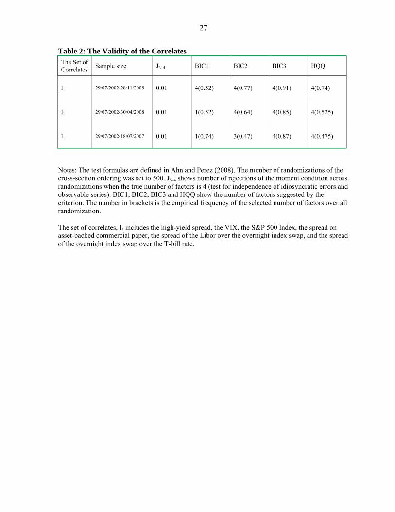
The GMM-based model and moment selection criterion of the validity of the
observed series is performed first and the results are presented in Table 2. The test is
performed for the full sample and two sub samples (up to July 2007 and up to May 2008) in
order to examine whether the most recent period (with possible outliers) is influencing the
results. In the first column of Table 2 we can see that none of the proposed series is
correlated with the idiosyncratic part of CDS spreads since the frequency of rejections of the
null among all randomizations of the data is very small for all samples. This implies that we
can use the moment selection criterion to investigate the relationship between the observed
series and the factors. In turn, the results from full and sub-sample estimation of the criterion
that finding a high correlation between the first factor and individual observed series cannot be an artifact of correlation between the other factor and that series. The same does not hold when the factors have a similar contribution to the overall variation in the data.
24 VIX is the implied volatility on the S&P 100 (OEX) option and is a widely used measure of global risk aversion.
25 As with the CDS data, all series are recursively filtered and checked for nonstationarity and are standardized prior to the estimation of the correlations.

18
suggest that the information in the set of observed series is correlated with the three or four
factor subspace and that the patterns followed by the individual series are not spurious.26
IV.3 The Real Economy Prior to the Subprime Crisis
In the “real economy” group, we consider three correlates. High-yield spreads (HYS,
spreads on bonds issued by less-than-investment-grade issuers) reflect increased corporate
default probabilities and do well in predicting short-term growth prospects (Mody and
Taylor, 2003). The S&P 500 average reflects the market’s perception of the economic
outlook, while the VIX is a measure of economic volatility embedded in stock price
movements.
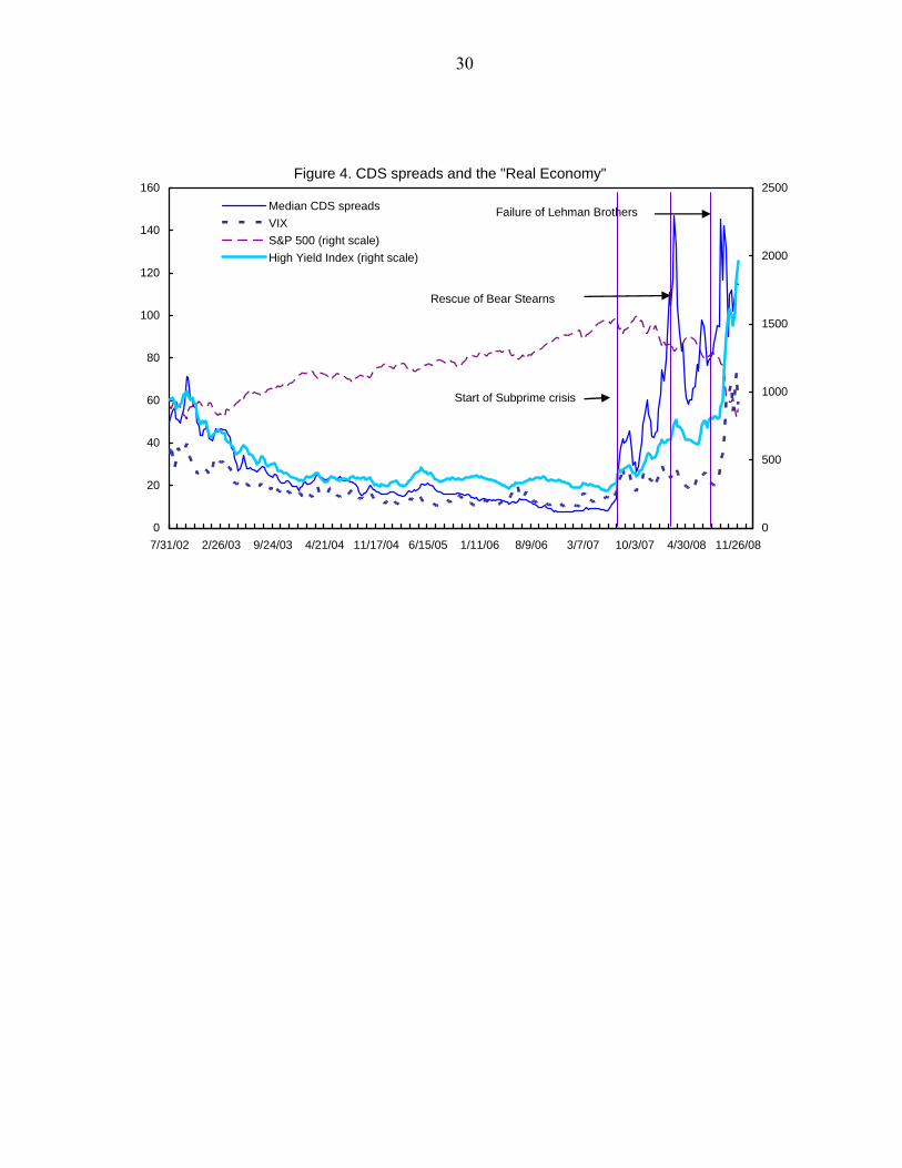
Figure 4 shows the evolution of (median) CDS spreads in relation to these observed
variables. Prior to the start of the subprime crisis, the HYS and the VIX trended down along
with the median CDS spreads. As the figure suggests and we show below, the real economy
as represented by the stock market bore less short-term relationship with the movement in
CDS spreads. The HYS, VIX, and CDS spreads were all at low levels prior to July 2007.
And while they rose subsequently, their short-term movements became less correlated
between the start of the subprime crisis and the failure of Lehman Brothers.
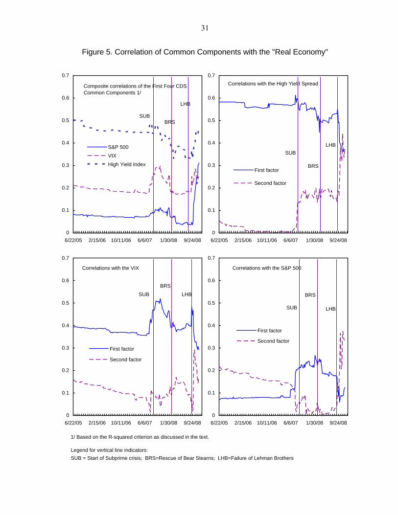
In Figure 5, panel A, we show the correlation of the first four factor space with HYS;
this was relatively high prior to the subprime crisis. The R-squared criterion gives a value of
0.5 on the eve of the subprime crisis. In contrast, the correlation with the S&P returns is
26 For the full sample, the various criteria suggest the existence of a relationship between the series and four factors. For the sub-samples BIC1 suggests a relationship with only one factor, whereas three or four factors are picked by other criterion. Given that apart from the first factor, all other factors may be perceived as weak, BIC1 may underselect the true number of relationships, as shown in the simulation study. On the other hand, BIC3 and HQQ tend to overselect the true number of relationships. As such we base our inference on BIC2.
19
low—the R-squared is less than 0.1. Notice that the R-squared for the VIX lies in between,
but at 0.2 is at the lower end of the range.
The implication is that perceptions of banks’ risk in that tranquil period were shaped
by a global factor that is best summarized by corporate default risk. This is reasonable not
just because of the banks’ direct exposure to default risk but also because HYS have a proven
track record as a forward-looking predictor of economic prospects (Mody and Taylor, 2003).
In particular, HYS movements capture the operation of the financial accelerator: high spreads
imply high expected default rates (and hence lower collateral), lower credit supply, reduced
growth prospects, and hence higher spreads. HYS has also been found to be a significant
explanatory variable of emerging market spread differences across countries and movements
over time (see Eichengreen and Mody, 2000, and Longstaff et al., 2008, who find it to be the
most potent of their candidate variables). In contrast, stock returns include both upside and
downside movements: while high stock returns presumably lower risk to a degree, banks’
risks are apparently more clearly defined by downside risks as reflected in the HYS. The fact
that the correlation with the VIX is significantly smaller than for HYS suggests that a
generalized risk aversion does not necessarily translate into banks’ risk premia.
These interpretations are supported by the correlations with specific factors reported
in Panel B of Figure 5. Up through the start of the subprime crisis, the HYS was most highly
correlated with the first principal component of CDS spreads.27 In contrast, there was almost
no correlation with the second factor. The same was true the VIX (panel C). In contrast, S&P
returns had a higher correlation with the second factor (panel D). An interpretation is that the
first factor reflects global perceptions of downside risks, while the second gives more weight 27 Hereafter, all the correlations are expressed in absolute terms for the ease of comparison.
20
to general movements in expected future profitability. Note, though, that the second factor
explains a much smaller fraction of the overall variance of CDS spreads. Hence returns had
a much weaker association with spreads’ movements.
IV.4 The Emergence of Financial Factors
Thus, prior to the subprime crisis, global economic factors as summarized in the HYS
were the main drivers of the CDS spreads of international banks. Following the onset of the
crisis and through the Bear Stearns bailout, however, the correlation with the HYS declined
(Figure 5, panel A). The decline in the overall correspondence between the HYS and the
factor space reflected a decline in correlation with the increasingly important first factor of
CDS spreads and occurred despite some increase in correlation with the second factor (panel
B). Evidently, there was some dissociation with the real economy despite the fact that banks’
prospects appear to have been perceived as increasingly correlated with one another in this
period. Intuitively, the common risk did not obviously emanate from a sense of worsening of
economic prospects. Moreover, an initial sharp increase in correlation with the VIX,
reflecting generalized risk aversion, died down to pre-crisis levels by the time of Bear
Stearns (Figure 5, panels A and C). The small rise in the correlation between S&P returns
and the CDS factor space probably reflects that that fears about the stability of the banking
system were driven more by problems in the banks’ positions in securities than by the ability
of their corporate customers to stay current on their loans.
Once the subprime crisis started, the relevance of financial variables, particularly
those related to banks’ credit and funding risks, acquired greater prominence. A common
metric of banks’ credit risks is the TED spread, or the difference between the interest rates on
21
interbank loans (we use the US dollar, 3-month LIBOR) and short-term U.S. government
debt (3-month US Treasury bills). This captures the risk premia on bank borrowing, since
LIBOR is the rate at which banks borrow and Treasury bills (T-Bills) are considered risk-
free.
However, the TED spread reflects not just banking sector credit risk but also includes
liquidity or flight-to-quality risk. These two categories of risks can be approximately
decomposed. TED=(LIBOR-OIS)+(OIS-“T-Bill”), where the OIS is an “overnight index
swap;” which measures the expected daily average Fed Funds rate over the next 3 months.
Thus, TED can be decomposed into the banking sector credit risk premium (LIBOR-OIS)
and liquidity or flight-to-quality premium (OIS-T-Bill).28
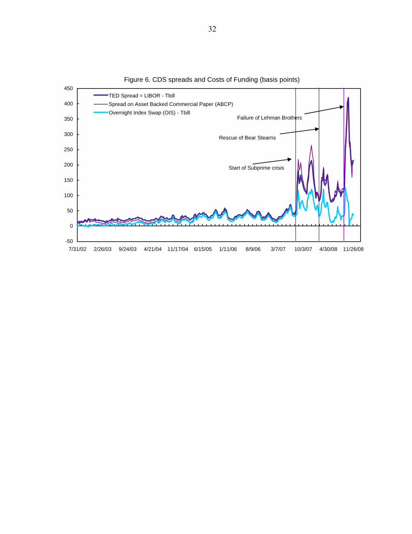
The TED spread rose sharply in the post-Lehman-crisis period as Figure 6 shows.
While the liquidity premium (the OIS-T-Bill differential) also increased, the more substantial
increase was in the credit risk (the LIBOR-OIS differential). Note also the spike after the
start of the subprime crisis in the spread on asset-backed commercial paper. Since banks use
these instruments for their short-term funding, the rise in this spread proxies the risks
associated with rollover in short-term funding. That the market for asset-backed commercial
paper issued by banks and conduits collapsed within days of the Lehman bankruptcy is well
known; see Jones (2009).29
28 Of course, the OIS-TB spread picks up some credit risk, but most analysts now view the “general collateral” repo rate as the “risk free” rate, and that plots very closely to the OIS rate. The LIBOR-OIS spread is analyzed by Taylor (2009) and critiqued by Jones (2009).
29 Note also from Figure 6 that the LIBOR-OIS spread moved rather closely with the spreads on asset-backed commercial paper, often used to proxy the banks’ costs of funding since banks issue such paper to fund their investments.

22
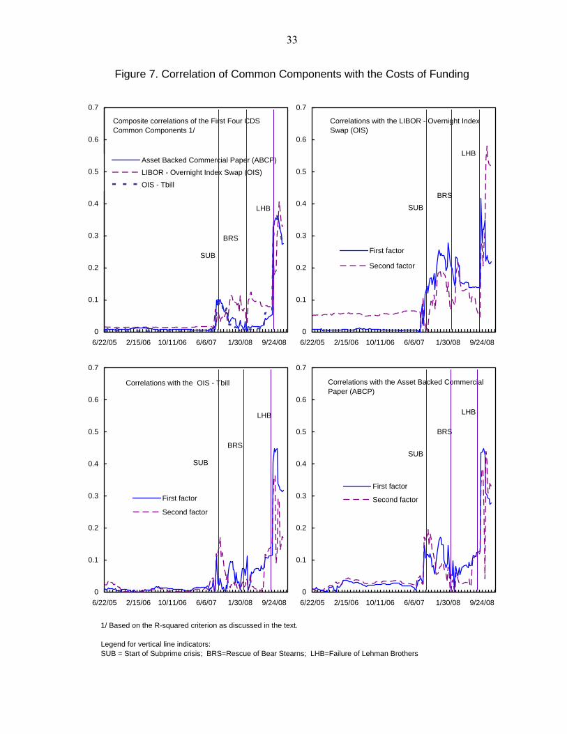
The correlation of the common factors with these financial variables, which had been
historically close to zero, rose following the start of the crisis (Figure 7). Thus perceived
bank risk, which had previously stemmed mainly from the development of the real economy,
now stemmed more from banks’ own internal credit and funding risks. But while liquidity
risk (as captured by the OIS-T-bill spread) and the ABCP spread showed some correlation
with the CDS factor space initially, those correlations were not sustained. In contrast, the
correlation with credit risk was sustained. Credit risk had the largest correlation of these three
financial variables with the factor space after the start of the crisis; in particular, the
correlation with the first factor rose steadily up until Bear Stearns.
While the change in the pattern of correlations clearly points to greater emphasis on
the internal workings of the banking system (rather than to the broader global economy), the
correlations we find even at their elevated levels during this phase are small.30 To the extent
that banks’ credit risk and funding risk did become more important, our measures for these
features may not be sufficiently encompassing. In addition other concerns, such as lack of
transparency of the complex asset holdings, may have also acquired greater prominence in
assessing bank risks.
Not much changed between the Bear Stearns rescue and the Lehman failure. The
correlation with HYS stabilized at below pre-crisis levels and the correlation with credit risk
remained significantly above pre-crisis levels. The other correlations remained low, near
their pre-crisis levels. Thus while corporate default risk remained a salient factor determining
30 Thus, to a degree the rise in the share of the first component (and first four components) of CDS spreads remains a matter for further investigation.
23
banks’ risk, there was a shift as this traditionally-dominant factor lost ground and the risk that
banks themselves may not be able to honor each others obligations gained prominence.
IV. 5 After Lehman
The immediate post-Lehman phase is remarkable for the unprecedented alignment of
risks. The correlation between the CDS factor space and all of their correlates rose, according
the R-squared criterion, with the correlations with the financial variables increasing most
sharply. The increase in credit and funding risk premia reflected the stress faced by banks. In
addition, these developments presumably contributed to a revision of prospects of the real
economy that further undermined confidence in the condition of and prospects for the
banking system.
By the R-squared criterion, the correlation between the space of common factors in
bank CDS spreads and the HYS increased following the failure of Lehman, reversing its
decline in the preceding four-plus quarters. The correlation with the S&P returns showed a
particularly large increase as global economic prospects were seen as increasingly tied to the
fortunes of banks. In contrast, despite the high level of VIX during this period, the correlation
between the CDS factor space and VIX increased relatively little. In contrast, there was an
especially sharp increase in the correlation between the financial variables and the common
factor in banks’ CDS spreads.
Differences in the correlations between these real and financial variables and the first
and second common factors provide further intuition. The financial stress indicators became
more correlated with the first factor of CDS spreads; that correlation rose to levels that had
not been seen before. In contrast, the real economic variables, particularly the HYS, that had
24
moved the first factor in the past, declined sharply in importance in the immediate post-
Lehman phase. Instead, the correlation between the real economy and the common CDS
movements shifted to the smaller, second factor.
V. CONCLUSIONS
We have analyzed common factors in bank credit default swaps both before and
during the credit crisis that broke out in July 2007 in order to better understand how this
crisis spread from the subprime segment of the U.S. financial market to the entire U.S. and
global banking system. We showed first common factors in CDS spreads are present even in
normal times; they reflect the impact of the macroeconomy—the ultimate common factor
from this point of view—on banks as a group. But the importance of the common factor
increased significantly between the eruption of the Subprime Crisis in July 2007 and the
failure of Lehman Brothers in September 2008. This increase in the common factor seems to
have been associated with a proxy for the banking-sector credit-risk premium, especially in
the period prior to the rescue of Bear Stearns. In contrast, the correlation with the state of the
real economy, which had been evident prior to the crisis, appears to have been somewhat
attenuated. In this abnormal period investors, in other words, investors were not yet
concerned so much with the prospect of a global recession that would impact the banks’ loan
books as with other credit risks affecting the banks – connected, presumably, with their
investments in subprime related securities.
After the failure of Lehman Brothers the importance of the common factor remained
elevated. But where movements in that factor had previously been related to diffuse
measures of generalized banking-sector credit risk, they now became increasingly linked to
25
measures of funding risk. In addition, the correlation of the common factor with the real
economy reasserted itself, as evidence of the deepening recession mounted.
What does this evidence imply for policy decisions taken in this period? With benefit
of hindsight (which is what a retrospective statistical analysis permits), we can see a
substantial common factor in banks’ CDS spreads that could have alerted the authorities to
the risks of allowing a major financial institution to fail. The further increase in that common
factor in the period between the outbreak of the Subprime Crisis and the critical decision
concerning Lehman Brothers should have implied further caution in this regard. It was not
the implications of any impending economic slowdown about which investors were primarily
worried in this period; rather the concern was about the state of the banks’ asset portfolios
and, presumably, their investments in securities in particular. The heightened comovement at
least in part reflected incomplete knowledge about the magnitude of toxic asset positions in
this relatively early stage of the crisis, and, hence, raised the possibility that instability could
spread more quickly and widely than assumed in the consensus view. In the event, Lehman
Brothers was allowed to fail, after which the sensitivity of the CDS spreads of global banks
as a group experienced heightened sensitivity to the whole range of economic and financial
variables. As those variables deteriorated, the result was a perfect storm.

26
Table 1: The Sample of Financial Institutions Mean Standard
deviation Median Minimum Maximum
Abbey 26.29 27.36 15.16 4.51 137.93 Barclays 28.45 37.81 12.21 5.65 251.89 HBOS 35.64 54.12 13.78 4.84 385.86 HSBC 23.73 23.88 14.01 4.99 134.96 Lloyds TSB 22.39 27.24 12.30 3.87 184.40 RBS 28.84 39.71 13.02 4.00 289.11 Standard Chartered 31.65 30.37 18.59 5.87 176.73 Allianz 36.19 27.76 24.92 6.03 136.59 Commerzbank 45.81 41.82 27.05 8.14 221.83 HVB 43.24 36.41 29.64 6.32 167.81 Deutsche Bank 31.38 28.54 18.29 10.11 161.68 Dresdner Bank 34.73 30.22 22.00 5.52 154.83 Hannover Rueckversicherung 44.88 30.08 34.67 8.17 138.25 Münchner Hypoth. 32.31 20.56 25.56 5.78 120.19 Monte dei Paschi 30.90 24.31 21.03 6.17 137.93 UniCredit 28.27 25.28 16.06 7.65 133.66 AXA 49.19 46.95 27.93 9.11 235.14 BNP Paribas 20.51 19.01 12.31 5.51 103.83 Credit Agricole 24.19 27.47 13.27 6.08 145.56 LCL 24.58 27.61 12.58 6.16 150.27 Société Générale 24.85 27.11 13.25 5.97 138.93 ABN AMRO 26.79 29.92 15.03 5.26 172.69 ING 26.54 31.12 15.44 4.45 163.93 Rabobank 16.83 22.49 8.35 3.12 131.92 Banco Santader 31.46 30.47 16.89 7.68 143.98 Credit Suisse 38.98 35.44 20.87 9.04 169.57 UBS 29.04 43.34 11.63 4.55 276.23 Banco Comerc. Port. 33.20 28.23 21.86 8.20 145.36 American Express 59.97 90.51 25.84 9.07 603.16 AIG 101.24 310.18 24.87 8.57 2624.15 Bank of America 35.03 33.93 21.34 8.47 191.45 Bear Sterns 60.14 62.51 34.47 19.01 574.31 Chubb 39.28 29.26 29.94 10.01 153.70 Citibank 43.19 54.79 20.83 7.52 351.93 Fed. Mortgage 22.81 14.09 20.67 6.35 82.55 Freddie Mac 21.77 14.77 19.03 5.28 83.10 Goldman Sachs 57.72 64.67 34.33 18.95 437.37 Hartford 67.82 111.88 36.36 10.82 826.17 JP Morgan 44.05 31.96 31.37 11.81 174.98 Lehman Brothers 86.00 127.03 36.74 19.49 641.91 Merrill Lynch 68.94 77.04 34.60 15.61 417.10 Met Life 62.58 108.22 30.46 11.20 790.42 Morgan Stanley 73.21 117.44 34.42 18.59 1153.09 Safeco 46.01 34.38 32.88 18.04 181.00 Wachovia 52.70 84.18 21.42 10.40 741.79
27
Table 2: The Validity of the Correlates The Set of Correlates Sample size JN-4 BIC1 BIC2 BIC3 HQQ
I1 29/07/2002-28/11/2008 0.01 4(0.52) 4(0.77) 4(0.91) 4(0.74)
I1 29/07/2002-30/04/2008 0.01 1(0.52) 4(0.64) 4(0.85) 4(0.525)
I1 29/07/2002-18/07/2007 0.01 1(0.74) 3(0.47) 4(0.87) 4(0.475)
Notes: The test formulas are defined in Ahn and Perez (2008). The number of randomizations of the cross-section ordering was set to 500. JN-4 shows number of rejections of the moment condition across randomizations when the true number of factors is 4 (test for independence of idiosyncratic errors and observable series). BIC1, BIC2, BIC3 and HQQ show the number of factors suggested by the criterion. The number in brackets is the empirical frequency of the selected number of factors over all randomization. The set of correlates, I1 includes the high-yield spread, the VIX, the S&P 500 Index, the spread on asset-backed commercial paper, the spread of the Libor over the overnight index swap, and the spread of the overnight index swap over the T-bill rate.

28
Figure 1. Evolution of Spreads on Credit Default Swaps (median, basis points)
0
50
100
150
200
250
300
350
400
450
7/31/02 2/26/03 9/24/03 4/21/04 11/17/04 6/15/05 1/11/06 8/9/06 3/7/07 10/3/07 4/30/08 11/26/08
All 45 banksEuropean banksU.S. banks
Start of Subprime crisis
Rescue of Bear Stearns
Failure of Lehman Brothers
Figure 2. Share of CDS Spreads'Variation Explained by the Four Common Components
30%
40%
50%
60%
70%
80%
90%
6/22/05 10/12/05 2/1/06 5/24/06 9/13/06 1/3/07 4/25/07 8/15/07 12/5/07 3/26/08 7/16/08 11/5/08
Contribution of third and four factorsContribution of second factorContribution of first factorSum of all four factors
Start of Subprime crisis
Rescue of Bear Stearns
Failure of Lehman Brothers
29
Figure 3. Additional Spillovers
(a) Fraction of Pairs of Banks Incurring "Additional" Spillovers
0%
1%
2%
3%
4%
5%
6%
6/22/05 10/12/05 2/1/06 5/24/06 9/13/06 1/3/07 4/25/07 8/15/07 12/5/07 3/26/08 7/16/08 11/5/08
Start of Subprime crisis
Failure of Lehman Brothers
Rescue of Bear Stearns
(b) Fraction of American Banks Facing Additional Spillovers from at least one European Bank
0%
10%
20%
30%
40%
50%
6/22/05 10/12/05 2/1/06 5/24/06 9/13/06 1/3/07 4/25/07 8/15/07 12/5/07 3/26/08 7/16/08 11/5/08
Start of Subprime crisisFailure of Lehman Brothers
Rescue of Bear Stearns
(c) Fraction of European Banks Facing Additional Spillovers from at least one American Bank
0%
10%
20%
30%
40%
6/22/05 10/12/05 2/1/06 5/24/06 9/13/06 1/3/07 4/25/07 8/15/07 12/5/07 3/26/08 7/16/08 11/5/08
Start of Subprime crisis
Failure of Lehman Brothers
Rescue of Bear Stearns
30
Figure 4. CDS spreads and the "Real Economy"
0
20
40
60
80
100
120
140
160
7/31/02 2/26/03 9/24/03 4/21/04 11/17/04 6/15/05 1/11/06 8/9/06 3/7/07 10/3/07 4/30/08 11/26/080
500
1000
1500
2000
2500Median CDS spreadsVIXS&P 500 (right scale)High Yield Index (right scale)
Start of Subprime crisis
Rescue of Bear Stearns
Failure of Lehman Brothers
31
Figure 5. Correlation of Common Components with the "Real Economy"
1/ Based on the R-squared criterion as discussed in the text.
Legend for vertical line indicators:SUB = Start of Subprime crisis; BRS=Rescue of Bear Stearns; LHB=Failure of Lehman Brothers
Composite correlations of the First Four CDS Common Components 1/
0
0.1
0.2
0.3
0.4
0.5
0.6
0.7
6/22/05 2/15/06 10/11/06 6/6/07 1/30/08 9/24/08
S&P 500
VIX
High Yield Index
SUBBRS
LHB
Correlations with the High Yield Spread
0
0.1
0.2
0.3
0.4
0.5
0.6
0.7
6/22/05 2/15/06 10/11/06 6/6/07 1/30/08 9/24/08
First factor
Second factor
SUB
BRS
LHB
Correlations with the VIX
0
0.1
0.2
0.3
0.4
0.5
0.6
0.7
6/22/05 2/15/06 10/11/06 6/6/07 1/30/08 9/24/08
First factor
Second factor
SUBBRS
LHB
Correlations with the S&P 500
0
0.1
0.2
0.3
0.4
0.5
0.6
0.7
6/22/05 2/15/06 10/11/06 6/6/07 1/30/08 9/24/08
First factor
Second factor
SUB
BRS
LHB
32
Figure 6. CDS spreads and Costs of Funding (basis points)
-50
0
50
100
150
200
250
300
350
400
450
7/31/02 2/26/03 9/24/03 4/21/04 11/17/04 6/15/05 1/11/06 8/9/06 3/7/07 10/3/07 4/30/08 11/26/08
TED Spread = LIBOR - TbillSpread on Asset Backed Commercial Paper (ABCP)Overnight Index Swap (OIS) - Tbill
Start of Subprime crisis
Rescue of Bear Stearns
Failure of Lehman Brothers
33
Figure 7. Correlation of Common Components with the Costs of Funding
1/ Based on the R-squared criterion as discussed in the text.
Legend for vertical line indicators:SUB = Start of Subprime crisis; BRS=Rescue of Bear Stearns; LHB=Failure of Lehman Brothers
Composite correlations of the First Four CDS Common Components 1/
0
0.1
0.2
0.3
0.4
0.5
0.6
0.7
6/22/05 2/15/06 10/11/06 6/6/07 1/30/08 9/24/08
Asset Backed Commercial Paper (ABCP)
LIBOR - Overnight Index Swap (OIS)
OIS - Tbill
SUB
BRS
LHB
Correlations with the LIBOR - Overnight Index Swap (OIS)
0
0.1
0.2
0.3
0.4
0.5
0.6
0.7
6/22/05 2/15/06 10/11/06 6/6/07 1/30/08 9/24/08
First factor
Second factor
SUBBRS
LHB
Correlations with the OIS - Tbill
0
0.1
0.2
0.3
0.4
0.5
0.6
0.7
6/22/05 2/15/06 10/11/06 6/6/07 1/30/08 9/24/08
First factor
Second factor
SUB
BRS
LHB
Correlations with the Asset Backed Commercial Paper (ABCP)
0
0.1
0.2
0.3
0.4
0.5
0.6
0.7
6/22/05 2/15/06 10/11/06 6/6/07 1/30/08 9/24/08
First factor
Second factor
SUB
BRS
LHB
34
References
Ahn, Seung and M. Fabrizio Perez, 2008, “GMM Estimation of the Number of Latent Factors”, Arizona State University mimeo.
Anderson, Helen and Farshid Vahid, 2007, “Forecasting the Volatility of Australian Stock
Returns: Do Common Factors Help?” Journal of Business and Economic Statistics 25(1), pp.76-90.
Andrews, Donald W.K. and Biao Lu, 2001, “Consistent model and moment selection
procedures for GMM estimation with application to dynamic panel data models”, Journal of Econometrics 101, pp 123-164.
Bai, Jushan and Serena Ng, 2002, “Determining the Number of Factors in Approximate
Factor Models”, Econometrica 70(1), pp. 191–221. Bai, Jushan and Serena Ng, 2006a, “Confidence Intervals for Diffusion Index Forecasts and
Inference with Factor-Augmented Regressions”, Econometrica 74(4), pp. 1133–1150. Bai, Jushan and Serena Ng, 2006b, “Evaluating Latent and Observed Factors in
Macroeconomics and Finance”, Journal of Econometrics 113, pp. 507–537. Bai, Jushan and Serena Ng, 2008, “Extremum Estimation when the Predictors are Estimated
from Large Panels”, Annals of Economics and Finance, 9(2), pp. 201-222 Brunnermeier, M.K. 2009, “Deciphering the Liquidity and Credit Crunch 2007-08,” Journal
of Economic Perspectives, forthcoming. Chamberlain, Garry and Michael Rothschild, 1983, “Arbitrage, Factor Structure and Mean-
Variance Analysis in Large Asset Markets”, Econometrica 51, pp. 1281–1304. Clark, Todd E. and Michael W. McCracken, 2005. "The power of tests of predictive ability in
the presence of structural breaks", Journal of Econometrics 124(1), pp 1-31, Davidson, Russell and James MacKinnon, 1985, “Heteroskedasticity-robust tests in
regression directions”, Annales de l’INSEE 59, pp. 183–218. Eichengreen, Barry and Ashoka Mody. 2000. “What explains changing spreads on emerging
market debt?” in Sebastian Edwards (ed.), Capital Flows and the Emerging Economies, Chicago: University of Chicago Press.
Goncalves, Silvia and Lutz Kilian, 2004, "Bootstrapping Autoregressions with Conditional
Heteroscedasticity of Unknown Form,” Journal of Econometrics 123, pp. 89-120. Hansen, Bruce, 2000, “Testing for structural change in conditional models”, Journal of
Econometrics 97, pp. 93-115.

35
Jones, Sam, 2009, “Why Letting Lehman Go Did Crush the Financial Markets,”
www.ft.com/alphaville (12 March). Longstaff, F.A., Pan, J., Pedersen, L.H. and Singleton, K.J. 2008, “How Sovereign Is
Sovereign Credit Risk?” UCLA and Stanford, mimeo. Mody, Ashoka and Mark Taylor, 2003, “The High Yield Spread as a Predictor of Real
Economic Activity: Evidence of a Financial Accelerator for the United States,” IMF Staff Papers 50(3): 373-402.
Onatski, Alexei, 2006, “Determining the Number of Factors from Empirical Distribution of Eigenvalues,” Columbia University mimeo. Rossi, Barbara, 2005, “Optimal Tests for Nested Model Selection with Underlying Parameter
Instability”, Econometric Theory 21, pp. 962-990. Soros, George, 2009, “The Game Changer,” Financial Times, January 28,
http://www.ft.com/cms/s/0/49b1654a-ed60-11dd-bd60-0000779fd2ac.html?nclick_check=1
Stock, James and Mark Watson, 2002, “Forecasting Using Principal Components from a Large Number of Predictors,” Journal of the American Statistical Association 97, pp. 1167-1179. Taylor, John B., 2009, Getting Off Track: How Government Actions and Interventions
Caused, Prolonged, and Worsened the Financial Crisis, Stanford, CA: Hoover Institution Press.
Zhang, Benjamin Yi-Bin, Zhou, Hao and Zhu, Haibin, 2008, “Explaining Credit Default
Swap Spreads With the Equity Volatility and Jump Risks of Individual Firms,” FEDS Discussion Paper No. 2005-63; Review of Financial Studies, Forthcoming; BIS Working Paper No. 181. Available at SSRN: http://ssrn.com/abstract=713482


