

IOSR Journal of Electrical and Electronics Engineering (IOSR-JEEE)
e-ISSN: 2278-1676,p-ISSN: 2320-3331, Volume 5, Issue 6 (May. - Jun. 2013), PP 55-80 www.iosrjournals.org
www.iosrjournals.org 55 | Page
Hydro-Thermal Scheduling: Using Soft Computing Technique
Approch
Sudipta Sen, Arka Roy (ELECTRICAL ENGINEERING / Techno India, India)
(ELECTRICAL ENGINEERING / Techno India, India)
Abstract: The project work HYDRO-THERMAL SCHEDULING is done to optimize generation cost of power
in a hydro-thermal power plant using MATLAB software. This is basically a simulation project. Here three
different types of techniques or algorithms have been used. These are classical method of solving short term
fixed head hydrothermal scheduling, Genetic algorithm and Differential Evolution method. Genetic algorithm is
a meta-heuristic search method and Differential Evolution is another method which makes the results better by
generation to generation. Here the results of all these algorithms and methods are compared and the best result
is obtained to optimize the cost function.
For performing the comparative study among the three methods the help of the software MATLAB has
been taken as a tool for coding. This study is being performed on a primitive hydro-thermal power system
network consisting of one thermal power plant and one hydel power plant. Genetic algorithm has emerged as a
candidate due to its flexibility and efficiency for many optimization applications. DE or differential evolution belongs to the class of evolutionary algorithms that include evolution strategies (ES) and conventional genetic
algorithms (GA).
Keywords – [1] Classical Method [2] Differential Evolution [3] Generic Algorithm [ 4] Hydro-Thermal
Scheduling [5]MATLAB
I. Introduction A modern power system consists of a large number of thermal and hydel power plants connected at
various load centers through a transmission network. An important objective in the operation of such a power
system is to generate and transmit power to meet the system load demand at minimum fuel cost by an optimal
mix of various types of plants. The study of the problem of optimal scheduling of power generation at various plants in a power system is of paramount importance, particularly where the hydel sources are scarce and high
cost of thermal generation has to be relied upon to meet the power demand. The hydel resources being
extremely limited , the worth water is greatly increased. If optimum use is made of their limited resources in
conjunction with the thermal sources, huge saving in fuel and the associated cost can be made.
In certain sectors, however, the hydel source is sufficiently large, particularly in rainy seasons as the
inflows into the hydel exhibit an annual cyclicity. Moreover there may be a seasonal variation in power demand
on the system, and this too exhibits an annual cyclicity. The optimization interval of one year is thus a natural
choice for long range optimal generation scheduling. The solution to the scheduling problem in this case
consists of determination of water quantities to be drawn from the reservoirs for hydel generation in each sub-
interval and the corresponding thermal generation to meet the load demand over each sub-interval utilizing the
entire quantity of water available for power generation during the total interval. The long range scheduling (generally persisting from months to year) involves mainly the scheduling of water release. Long range
scheduling also involves meteorological and statistical analysis. The benefit of this scheduling is to save the cost
of generation, in addition to meeting the agricultural and irrigational requirements. Long range scheduling
involves optimization of the operating policy in the context of major unknowns such as load, hydroelectric
inflows, unit availability etc.
The short range problem usually has an optimization interval of a day or a week. This period is
normally divided into sub-intervals for scheduled purposes. Here the load, water inflows and unit availability are
assumed to be known. A set of starting conditions being given, an optimal hourly schedule can be prepared that
minimizes a desired objective while meeting system constraints successfully.
Cost optimization of hydro stations can be achieved by assuming the water head constant and
converting the incremental water rate characteristics to incremental fuel cost curve by multiplying it with the
cost of water per cubic meter and applying the conventional technique of minimizing the cost function.

Hydro-Thermal Scheduling: Using Soft Computing Technique Approch
www.iosrjournals.org 56 | Page
Problem Definition Short term fixed head hydro-thermal scheduling considering transmission line loss and involving
multiple thermal and hydro generators for minimizing thermal generation cost and optimal use of limited water
resource available.
The endeavor of this project is to perform a comparative study of the results obtained by solving the
hydro-thermal scheduling problem with the help the Classical method, the Genetic Algorithm and the
Differential Evolutionary Algorithm and draw a conclusion about their effectivity in solving this optimization
problem.
A hydro thermal system consists of one thermal and one hydro unit. The units have following characteristics.
Hydro plant: W=(0.2 2.5 +1.5* ) /hr
Volume of water available=42*
Thermal plant : =(0.002 +10 +1000) unit of cost/MW
Prepare a hydrothermal schedule per hour basis for the same plant for one day, where the load has the following
schedule:
12 midnight-12 noon :350 MW, 12 noon-12 midnight:700 MW
Consider and
The B-coefficient matrix of the system is
= *
Planning and Approach For performing the comparative study among the three methods the help of the software MATLAB has
been taken as a tool for coding. This study is being performed on a primitive hydro-thermal power system
network consisting of one thermal power plant and one hydel power plant.
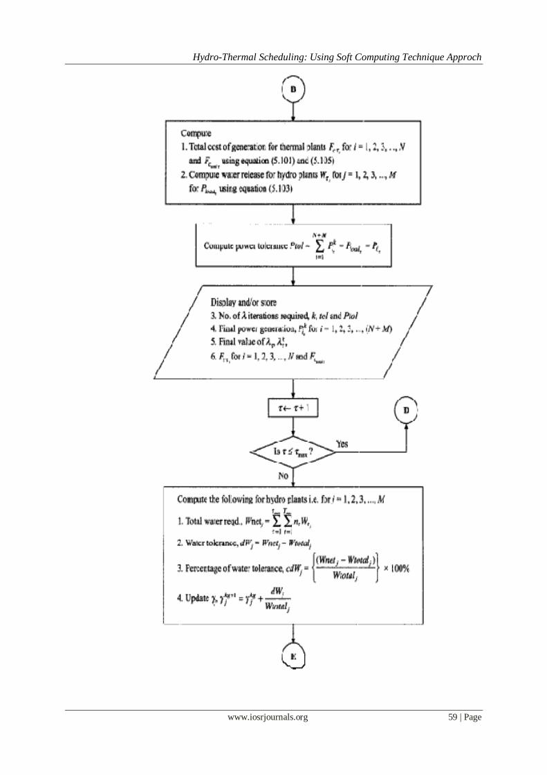
Fig 1

Hydro-Thermal Scheduling: Using Soft Computing Technique Approch
www.iosrjournals.org 57 | Page
1.1 Classical Method

Hydro-Thermal Scheduling: Using Soft Computing Technique Approch
www.iosrjournals.org 58 | Page
Hydro-Thermal Scheduling: Using Soft Computing Technique Approch
www.iosrjournals.org 59 | Page

Hydro-Thermal Scheduling: Using Soft Computing Technique Approch
www.iosrjournals.org 60 | Page
Fig 2
1.2 Genetic Algorithm A global optimization technique known as genetic algorithm has emerged as a candidate due to its
flexibility and efficiency for many optimization applications. Genetic algorithm is a stochastic searching
algorithm. It combines an artificial ,i.e., the Darwinian survival of the fittest principle of genetic operation,
abstracted from nature to form a robust mechanism that is very effective at finding optimal solutions to complex
real world problems. Evolutionary computing is an adaptive search technique based on the principles of genetics
and natural selection. They operate on string structures. The string is a combination of binary digits representing
a coding of the control parameters of a given problem. Many such string structures are considered
simultaneously, with the most fit of these structures receiving exponentially increasing opportunities to pass on genetically important material to successive generation of string structures. In this way genetic algorithms
search for many points is the search space at once, and yet continually narrow the focus of the search to the
areas of the observed best performance. The basic elements of genetic algorithms are reproduction, crossover
and mutation.
The first step is the coding of control variables as strings in binary numbers. In reproduction the individuals are
selected based on their fitness values relative to those of population. In the crossover operation, the two
individuals strings are selected at random from the mating pool and a crossover site is selected at random from
the mating pool and a crossover site is selected at random along the string length. The binary digits are
interchanged between two strings at crossover site. In Mutation, an occasional random alteration of a binary
digit Is done. The above procedure to implement genetic algorithms is outlined below:
Algorithm: Genetic Algorithm 1. Code the problem variables into binary strings.
2. Randomly generate initial population strings. Tossing of a coin can be used.
3. Evaluate fitness values of population members.
4. Is solution available among the population?
If yes GOTO step 9.
5. Select highly fit strings as parents and produce off springs according to their fitness.

Hydro-Thermal Scheduling: Using Soft Computing Technique Approch
www.iosrjournals.org 61 | Page
6. Create new strings by mating current off spring. Apply crossover and mutation operators to introduce
variations and form new strings.
7. New strings replace existing one. 8. GOTO step 4 ad repeat.
9. Stop.
Genetic algorithms are computerized search and optimization algorithms based on the principles of
natural genetics and natural selection. Although genetic algorithm were first presented systematically by prof.
John Holland of the university of Michigan, the basic ideas of analysis and design based on the concept of
biological evolution can be found in the work of Goldberg.
Hydrothermal Scheduling Using Genetic Algorithm:-
1.Read data, namely cost coefficients, ai, bi, ci, B-coefficients, Bij(i=1,2,3,….,NG; j=1,2,3,……NG),number of
steps for gamma correction (d), number of generations(z),step size α, water availability throughout all intervals q, l length of string, L population size, pc crossover probability, pm mutation probability, number of intervals (t),
λmin and λmax for each intervals etc.
2. Generate an array of random numbers. Generate the population λj (j=1, 2,…..L) by flipping the coin for both
intervals. The bit is set according to the coin flip as bij =1 if p=1 or 0<=p otherwise bij=0 where p=0.5.
3. Generate the initial population of gamma.
4. If number of iterations for gamma correction>= d then GOTO step 24 else repeat step 4 to 23.
5. If number of intervals <= t repeat step 6 to 20 for each interval and increment interval counter each time else
GOTO step 4.
6. Set the generation counter k=0, fmax=0 and fmin=1.
7. If k>=z GOTO step 5 else repeat step 7 to 20.
8. Increment generation counter k=k+1, and set population counter j=0.
9. Increment the population counter j=j+1.
10.Decode the string using the equations (j=1,2,……,L) and
+ /(2l-1) (j=1,2,…….,L).
11. Use Gauss Elimination method to find Pij (i=1,2,……NG including hydel and thermal generators).
12. Calculate the transmission loss.
13. Find out εj. 14. Find out the fitness values from the fitness function fj=1/(1+α*εj
/Pd). If (fj>fmax) then set fmax= fj and if
((fj<fmin) then set fmin= fj.
15. If (j<L) then GOTO step 9 and repeat.
16. Find population with maximum fitness and average fitness of the population.
17. Select the parents for crossover using stochastic remainder roulette wheel selection using the following
algorithm:
{ STOCHASTIC REMAINDER ROULETTE WHEEL SELECTION:
1. Input the fitness values of all individuals, (i=1, 2,……,L), population size, L.
2. Initialize the population counter, i=0 and initialize the selection counter, j=0.
3. Increment the selection counter, j=j+1.
4. Find y=
5. Separate the integer part of Y real number, I=integer(Y).
6. Separate the fractional part of Y, .
7. If (I<0) then GOTO step 12.
8. Increment the population counter, k=k+1.
9. Decrease the integer part to zero, I=I-1.
10. .
11. 7 and repeat.
12. Check, if (j>L) GOTO step 3 and repeat. 13. Reset the selection counter, j=0.
14. If (k>L) GOTO step 19.
15. Increment the selection counter, j=j+1.
16. If (j>L) then set j=1.
17. If ( >0.0) then {W=iflip( )}. If (W=1) then {k=k+1, , }

Hydro-Thermal Scheduling: Using Soft Computing Technique Approch
www.iosrjournals.org 62 | Page
18. GOTO step 14 and repeat.
19. Stop.
}
18. Perform single point crossover for the selected parents.
19. Perform the mutation.
20. Modify and create the new population of lambda for the next generation.
21. Check whether the total available water is enough for hydel generation in each interval.
22. Calculate the error in initially anticipated values of gammas’ population.
23. Modify the values of gamma in gammas’ population and GOTO step 4.
24. Stop.
1.3 Differential Evolution (DE) DE or differential evolution belongs to the class of evolutionary algorithms that include evolution
strategies (ES) and conventional genetic algorithms (GA). DE differs from the conventional genetic algorithms
in its use of perturbing vectors, which are the difference between two randomly chosen vectors. DE is a scheme
which it generates the trial vectors from a set of initial populations. In each step, DE mutates vectors by adding
weighted random vectors differentials to them. If the fitness of the trial vector is better than that of the target
vector, the trial vector replaces the target vector in the next generation.
DE offers several strategies for optimization. They are classified according to the following notations
such as DE/x/y/z, where x refers to the method used for generating parent vector that will form the base for
mutated vector, y indicates the number of difference vector used in mutation process and z is the crossover
scheme used in the cross over operation to create the offspring population. The symbol x can be ‘rand’ (randomly chosen vector) or ‘best’ (the best vector found so far). The symbol y i.e. the number of difference
vector, is normally set to be 1 or 2. For cross over operation, a binomial (notation: ‘bin’) or exponential
(notation: ‘exp’) operation is used. The version used here is the DE/rand/1/bin, which is described by the
following steps:
1.3.1 Initialization The optimization process in DE is carried with four basic operations: initialization, mutation, crossover
and selection. The algorithm starts by creating a population vector P of size Np composed of individuals that
evolve over G generation. Each individual Xi is a vector that contains as many as elements as the problem decision variable. The population size Np is an algorithm control parameter selected by the user. Thus
P(G) = [ (G)Xi ,……., (G)XNp ] (G)Xi = [ (G)Xi ,……, (G)XD,i ]
T, i= 1,……, Np
The initial population is chosen randomly in order to cover the entire searching region uniformly. A uniform
probability distribution for all random variables is assumed in the following as (0)Xj,I = minXj + σj(
maxXj – minXj )
Where i= 1,….., Np and j= 1,….., D.
Here D is the number of decision or control variable s, minXj and maxXj are the lower and upper limits of
the j the decision variables and σj є [0,1] is a uniformly distributed random number generated a new for each
value of j. (0)Xj,I is the jth parameter of the ith individual of the initial population.
1.3.2 Mutation operation Several strategies of mutation have been introduced in the literature of DE. The essential ingredient in
the mutation operation is the vector difference. The mutation operation creates mutant vectors (Vi) by perturbing
a randomly selected vector (Xk) with the difference of two other randomly selected vectors ( Xt and Xm )
according to (G)Vi = (G)Xk + fm( (G)Xl – (G)Xm )
where Xk, Xl and Xm are randomly chosen vectors є [1 ,….., Np] and k # l # m # i. In other words, the indices are
mutually different including the running index i. The mutation factor fm that lies within [0,2] is a user chosen
parameter used to control the perturbation size in the mutation operator and to avoid search stagnation.
1.3.3 Crossover operation In order to extend further diversity in the searching process, crossover operation is performed. The
crossover operation generates trial vectors (Ui) by mixing the parameter of the mutant vectors with the target
vectors. For each mutant vector, in index q є [ 1 ,……, Np ] is chosen randomly using a uniform distribution and
trial vectors are generated according to

Hydro-Thermal Scheduling: Using Soft Computing Technique Approch
www.iosrjournals.org 63 | Page
(G)Uj.i = (G)Vj,i , if ηj ≤ Cr or j=q.
= (G)Xj,i , otherwise.
Where i= 1 ,…….., Np and j= 1 ,….. D. ηj is a uniformly distributed random number within [0,1] generated anew for each value of j. The crossover factor CR є [0,1] is a user chosen parameter that controls the diversity of
the population. (G)Xj,i , (G)Vj,i and (G)Uj,i are the jth parameter of the ith target vector, mutant vector and trial
vector at G generation, respectively.
1.3.4 Selection operation Selection is the operation through which better offspring are generated. The evaluation (fitness)
function of an offspring is compared to that of its parent. The parent is replaced by its offspring if the fitness of
the offspring is better than that of its parent. While the parent is retained in the next generation if the fitness of
the offspring is worse than that of its parent. Thus , if f denotes the cost (fitness) function under optimization
(minimization), then (G+1)Xi =
(G)Ui , if f((G)Ui) ≤ f((G)Xi)
= (G)xi , otherwise.
The optimization process is repeated for several generations. This allows individuals to improve their fitness
while exploring the solution space for optimal value. The iterative process of mutation, crossover and selection
on the population will continue until a user-specified stopping criterion, normally, the maximum number of
generations allowed, is met. The other type of stopping criterion i.e. convergence to global optimum is possible
if the global optimum of the problem is available. Keeping all these into consideration, the DE technique has
been applied to solve the short-term combined economic emission scheduling problem of hydrothermal systems.
II. Design Issues The following assumptions are taken into consideration while designing the problem
1.4 Hydro reservoir has constant head during operation.
4.2 The water spillage from the water reservoir has been neglected. 4.3 The operating schedule is for 24 hours while each interval is for one hour.
4.4 The beginning and ending storage volumes are specified.
III. Testing
In this section MATLAB program code is given of different procedures:
1.5 Hydrothermal Scheduling using Genetic Algorithm f=[.2 2.5 15000 ; .002 10 1000];
%the first row describes the water rate characteristics of the hydal plant.
%the second row describes the fuel cost characteristics of the thermal
%plant.
p1max=700;
p1min=50;
p2max=700;
p2min=100; b=[4.45 -.05; -.05 4.5]*10^(-5);%B-coefficient matrix
l=22;%String Length
pop=20;%pop= number of population
pc=.8;%Crossover probability
pm=.01;%Mutation probability
p=.5;%Probability for creating random binary string
pd1=350;%Load demand during first interval
pd2=700;%Load demand during second interval
%Limits of lamda during the two interval
lamdamin1=11;
lamdamax1=11.5; lamdamin2=12.9;
lamdamax2=13.3;
%Maximum and minimum values of fitness function
fmin1=1;
fmax1=0;
fmin2=1;

Hydro-Thermal Scheduling: Using Soft Computing Technique Approch
www.iosrjournals.org 64 | Page
fmax2=0;
%Random binary string generation
for i=1:20, for j=1:22,
if rand<=p,
binstr(i,j)=1;
elseif rand==1,
binstr(i,j)=1;
else
binstr(i,j)=0;
end
end
end
binstr; %The binary string is converted to analog values
y=zeros(20,1);
for i=1:20,
for j=1:22,
y(i,1)=binstr(i,j)*2^(j-1)+y(i,1);
end
end
y;
%Creating the initial population of lamda for both intervals
lamda1=zeros(20,1);
for i=1:20,
lamda1(i,1)=lamdamin1+((lamdamax1-lamdamin1)*y(i,1))/(2^l-1); end
lamda1;
lamdaavg1=sum(lamda1)/20;
lamda2=zeros(20,1);
for i=1:20,
lamda2(i,1)=lamdamin2+((lamdamax2-lamdamin2)*y(i,1))/(2^l-1);
end
lamda2;
lamdaavg2=sum(lamda2)/20;
%Creating the initial population of gamma
gamma=zeros(20,1); for i=1:20,
gamma(i,1)=lamda1(i,1)/(2*f(1,1)*175+2.5);
end
for d=1:25,%Loop for corrction of gamma values
%.........Calculation during 1st interval........%
for z=1:50,%Loop for creating new generations for better results
%Creating elements of the matirx for obtaining the set of
%solution for each member of the population
for i=1:20,
a11(i,1)=2*(gamma(i,1)*f(1,1)+lamda1(i,1)*b(1,1));
end
a11; for i=1:20,
a22(i,1)=2*(f(2,1)+lamda1(i,1)*b(2,2));
end
a22;
for i=1:20,
a12(i,1)=2*b(1,2)*lamda1(i,1);
end
a21=a12;
for i=1:20,
c1(i,1)=lamda1(i,1)-f(1,2)*gamma(i,1);

Hydro-Thermal Scheduling: Using Soft Computing Technique Approch
www.iosrjournals.org 65 | Page
end
c1;
for i=1:20, c2(i,1)=lamda1(i,1)-f(2,2);
end
c2;
p1=zeros(3,20);
for i=1:20,
p1=inv([a11(i,1) a12(i,1); a21(i,1) a22(i,1)])*([c1(i);c2(i)]);
for j=1:2,
pp1(j,i)=p1(j,1);
end
end
pp1; for s=1:20,
if pp1(1,i)>p1max,
pp1(1,i)=p1max;
elseif pp1(1,i)<p1min,
pp1(i,1)=p1min;
else
end
if pp1(2,i)>p2max,
pp1(2,i)=p2max;
elseif pp1(2,i)<p2min,
pp1(2,i)=p2min;
else end
end
%Loop for calculating transmission loss
pl1=zeros(20,1);
for i=1:20,
for j=1:2,
for k=1:2,
pl1(i,1)=pl1(i,1)+pp1(k,i)'*b(k,j)*pp1(k,i);
end
end
end pl1;
%Loop for calculating the error in solution
eps1=zeros(20,1);
for i=1:20,
ppi1=0;
for j=1:2,
ppi1=pp1(j,i)+ppi1;
end
if (pd1+pl1(i,1))>ppi1,
eps1(i,1)=pd1+pl1(i,1)-ppi1;
else
eps1(i,1)=ppi1-pd1-pl1(i,1); end
end
eps1;
%Loop for calculating values
%Fitness function is 1/(1+eps1/pd1)
ff1=zeros(20,1);
for i=1:20,
ff1(i,1)=1/(1+eps1(i,1)/pd1);
if ff1(i,1)>fmax1,
fmax1=ff1(i,1);

Hydro-Thermal Scheduling: Using Soft Computing Technique Approch
www.iosrjournals.org 66 | Page
powerhydal1=pp1(1,i);
powerthermal1=pp1(2,i);
powerloss1=pl1(i,1); end
if ff1(i,1)<fmin1,
fmin1=ff1(i,1);
end
end
ff1;
avgff1=sum(ff1)/20;
i=0;
j=0;
%Stochastic remainder roulette wheel selection of strings
%available for crossover while j<20,
j=j+1;
y=ff1(j,1)/avgff1;
if y>=1,
integery=1;
else
integery=0;
end
frac(j,1)=y-1;
while integery>=0,
i=i+1;
integery=integery-1; sel1(i)=j;
end
end
sel1;
for i=1:20,
selstr1(i,1)=sel1(i);
end
selstr1;
%Crassover logic
for i=1:10,
p=1+round((20-i)*rand); q=selstr1(p);
r=1+round((20-i-1)*rand);
s=selstr1(r);
t=1+round((21-1+1)*rand);
for j=1:t,
binstr1(i,j)=binstr(q,j);
binstr1(i+10,j)=binstr(s,j);
end
for j=(t+1):22,
binstr1(i,j)=binstr(s,j);
binstr1(i+10,j)=binstr(q,j);
end end
%Mutation logic
for i=1:20,
for j=1:22,
if rand==1,
binstr1(i,j)=not(binstr1(i,j));
elseif rand<=pm,
binstr1(i,j)=not(binstr1(i,j));
else
binstr1(i,j)=binstr1(i,j);

Hydro-Thermal Scheduling: Using Soft Computing Technique Approch
www.iosrjournals.org 67 | Page
end
end
end binstr1;
binstr=binstr1;
y=zeros(20,1);
%Modified analog values of binary string
for i=1:20,
for j=1:22,
y(i,1)=binstr(i,j)*2^(j-1)+y(i,1);
end
end
y;
%Updating value of lamda lamda1=zeros(20,1);
for i=1:20,
lamda1(i,1)=lamdamin1+((lamdamax1-lamdamin1)*y(i,1))/(2^l-1);
end
lamda1;
lamdaavg1=sum(lamda1)/20;
end
%..........Calculation during 2nd interval..........%
%All the notations are same as 1st interval with a 2 suffix instead of 1
%where required%
for z=1:50,
for i=1:20, a11(i,1)=2*(gamma(i,1)*f(1,1)+lamda2(i,1)*b(1,1));
end
a11;
for i=1:20,
a22(i,1)=2*(f(2,1)+lamda2(i,1)*b(2,2));
end
a22;
for i=1:20,
a12(i,1)=2*b(1,2)*lamda2(i,1);
end
a21=a12; for i=1:20,
c1(i,1)=lamda2(i,1)-f(1,2)*gamma(i,1);
end
c1;
for i=1:20,
c2(i,1)=lamda2(i,1)-f(2,2);
end
c2;
p2=zeros(3,20);
for i=1:20,
p2=inv([a11(i,1) a12(i,1); a21(i,1) a22(i,1)])*([c1(i);c2(i)]);
for j=1:2, pp2(j,i)=p2(j,1);
end
end
pp2;
for s=1:20,
if pp2(1,i)>p1max,
pp2(1,i)=p1max;
elseif pp1(1,i)<p1min,
pp2(i,1)=p1min;
else

Hydro-Thermal Scheduling: Using Soft Computing Technique Approch
www.iosrjournals.org 68 | Page
end
if pp2(2,i)>p2max,
pp2(2,i)=p2max; elseif pp2(2,i)<p2min,
pp2(2,i)=p2min;
else
end
end
pl2=zeros(20,1);
for i=1:20,
for j=1:2,
for k=1:2,
pl2(i,1)=pl2(i,1)+pp2(k,i)'*b(k,j)*pp2(k,i);
end end
end
pl2;
eps2=zeros(20,1);
for i=1:20,
ppi2=0;
for j=1:2,
ppi2=pp2(j,i)+ppi2;
end
if (pd2+pl2(i,1))>ppi2,
eps2(i,1)=pd2+pl2(i,1)-ppi2;
else eps2(i,1)=ppi2-pd2-pl2(i,1);
end
end
eps2;
ff2=zeros(20,1);
for i=1:20,
ff2(i,1)=1/(1+eps2(i,1)/pd2);
if ff2(i,1)>fmax2,
fmax2=ff2(i,1);
powerhydal2=pp2(1,i);
powerthermal2=pp2(2,i); powerloss2=pl2(i,1);
end
if ff2(i,1)<fmin2,
fmin2=ff2(i,1);
end
end
ff2;
avgff2=sum(ff2)/20;
i=0;
j=0;
while j<20,
j=j+1; y=ff2(j,1)/avgff2;
if y>=1,
integery=1;
else
integery=0;
end
frac(j,1)=y-1;
while integery>=0,
i=i+1;
integery=integery-1;

Hydro-Thermal Scheduling: Using Soft Computing Technique Approch
www.iosrjournals.org 69 | Page
sel2(i)=j;
end
end sel2;
for i=1:20,
selstr2(i,1)=sel2(i);
end
selstr2;
for i=1:10,
p=1+round((20-i)*rand);
q=selstr2(p);
r=1+round((20-i-1)*rand);
s=selstr2(r);
t=1+round((21-1+1)*rand); for j=1:t,
binstr1(i,j)=binstr(q,j);
binstr1(i+10,j)=binstr(s,j);
end
for j=(t+1):22,
binstr1(i,j)=binstr(s,j);
binstr1(i+10,j)=binstr(q,j);
end
end
for i=1:20,
for j=1:22, if rand==1,
binstr1(i,j)=not(binstr1(i,j));
elseif rand<=pm,
binstr1(i,j)=not(binstr1(i,j));
else
binstr1(i,j)=binstr1(i,j);
end
end
end
binstr1;
binstr=binstr1; y=zeros(20,1);
for i=1:20,
for j=1:22,
y(i,1)=binstr(i,j)*2^(j-1)+y(i,1);
end
end
y;
lamda2=zeros(20,1);
for i=1:20,
lamda2(i,1)=lamdamin2+((lamdamax2-lamdamin2)*y(i,1))/(2^l-1);
end
lamda2; lamdaavg2=sum(lamda2)/20;
end
%The following loop is for correcting values of gamma
for i=1:20,
waterneed1(i,1)=.2*(pp1(1,i))^2+2.5*pp1(1,i)+15000;
waterneed2(i,1)=.2*(pp2(1,i))^2+2.5*pp2(1,i)+15000;
deltawater(i,1)=waterneed1(i,1)*12+waterneed2(i,1)*12-420000;
deltagamma(i,1)=deltawater(i,1)/420000;
gamma(i,1)=gamma(i,1)+deltagamma(i,1);
end
Hydro-Thermal Scheduling: Using Soft Computing Technique Approch
www.iosrjournals.org 70 | Page
end
avgpowerhydal1=0;
avgpowerthermal1=0; avgpowerhydal2=0;
avgpowerthermal2=0;
%The following loop is for calculating average values of thermal and hydal
%generation during each interval
for i=1:20,
avgpowerhydal1=avgpowerhydal1+pp1(1,i)/20;
avgpowerthermal1=avgpowerthermal1+pp1(2,i)/20;
avgpowerhydal2=avgpowerhydal2+pp2(1,i)/20;
avgpowerthermal2=avgpowerthermal2+pp2(2,i)/20;
end
avgpowerhydal1%Hydal generation during interval 1 avgpowerthermal1%Thermal generation during interval 1
avgpowerhydal2%Hydal generation during interval 2
avgpowerthermal2%Thermal generation during interval 2
averageloss1=sum(pl1)/20%Transmission loss during interval 1
averageloss2=sum(pl2)/20%Transmission loss during interval 2
%Thermal generation cost during 1st interval
rupees1=f(2,1)*avgpowerthermal1^2+f(2,2)*avgpowerthermal1+1000
%Thermal of thermal generation during 2nd interval
rupees2=f(2,1)*avgpowerthermal2^2+f(2,2)*avgpowerthermal2+1000
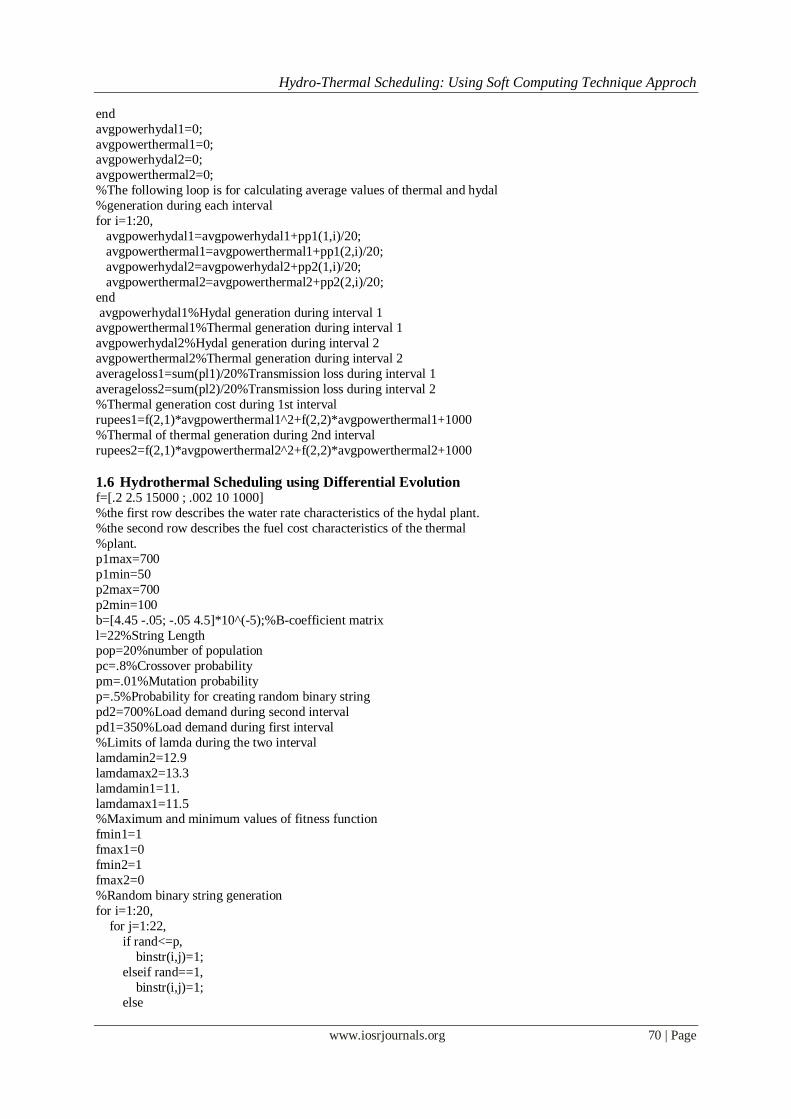
1.6 Hydrothermal Scheduling using Differential Evolution f=[.2 2.5 15000 ; .002 10 1000]
%the first row describes the water rate characteristics of the hydal plant.
%the second row describes the fuel cost characteristics of the thermal
%plant.
p1max=700
p1min=50
p2max=700
p2min=100
b=[4.45 -.05; -.05 4.5]*10^(-5);%B-coefficient matrix
l=22%String Length pop=20%number of population
pc=.8%Crossover probability
pm=.01%Mutation probability
p=.5%Probability for creating random binary string
pd2=700%Load demand during second interval
pd1=350%Load demand during first interval
%Limits of lamda during the two interval
lamdamin2=12.9
lamdamax2=13.3
lamdamin1=11.
lamdamax1=11.5 %Maximum and minimum values of fitness function
fmin1=1
fmax1=0
fmin2=1
fmax2=0
%Random binary string generation
for i=1:20,
for j=1:22,
if rand<=p,
binstr(i,j)=1;
elseif rand==1,
binstr(i,j)=1; else

Hydro-Thermal Scheduling: Using Soft Computing Technique Approch
www.iosrjournals.org 71 | Page
binstr(i,j)=0;
end
end end
binstr;
%The binary string is converted to analog values
y=zeros(20,1);
for i=1:20,
for j=1:22,
y(i,1)=binstr(i,j)*2^(j-1)+y(i,1);
end
end
y;
%Creating the initial population of lamda for both intervals lamda1=zeros(20,1);
for i=1:20,
lamda1(i,1)=lamdamin1+((lamdamax1-lamdamin1)*y(i,1))/(2^l-1);
end
lamda1;
lamdaavg1=sum(lamda1)/20;
lamda2=zeros(20,1);
for i=1:20,
lamda2(i,1)=lamdamin2+((lamdamax2-lamdamin2)*y(i,1))/(2^l-1);
end
lamda2;
lamdaavg2=sum(lamda2)/20; %Creating the initial population of gamma
gamma=zeros(20,1);
for i=1:20,
gamma(i,1)=lamda1(i,1)/(2*f(1,1)*175+2.5);
end
for d=1:8,%Loop for corrction of gamma values
%.........Calculation during 1st interval........%
for z=1:25,%Loop for creating new generations for better results
%Creating elements of the matirx for obtaining the set of
%solution for each member of the population
for i=1:20, a11(i,1)=2*(gamma(i,1)*f(1,1)+lamda1(i,1)*b(1,1));
end
a11;
for i=1:20,
a22(i,1)=2*(f(2,1)+lamda1(i,1)*b(2,2));
end
a22;
for i=1:20,
a12(i,1)=2*b(1,2)*lamda1(i,1);
end
a21=a12;
for i=1:20, c1(i,1)=lamda1(i,1)-f(1,2)*gamma(i,1);
end
c1;
for i=1:20,
c2(i,1)=lamda1(i,1)-f(2,2);
end
c2;
p1=zeros(3,20);
for i=1:20,
p1=inv([a11(i,1) a12(i,1); a21(i,1) a22(i,1)])*([c1(i);c2(i)]);

Hydro-Thermal Scheduling: Using Soft Computing Technique Approch
www.iosrjournals.org 72 | Page
for j=1:2,
pp1(j,i)=p1(j,1);
end end
pp1;
for s=1:20,
if pp1(1,i)>p1max,
pp1(1,i)=p1max;
elseif pp1(1,i)<p1min,
pp1(i,1)=p1min;
else
end
if pp1(2,i)>p2max,
pp1(2,i)=p2max; elseif pp1(2,i)<p2min,
pp1(2,i)=p2min;
else
end
end
%Loop for calculating transmission loss
pl1=zeros(20,1);
for i=1:20,
for j=1:2,
for k=1:2,
pl1(i,1)=pl1(i,1)+pp1(k,i)'*b(k,j)*pp1(k,i);
end end
end
pl1;
%Loop for calculating the error in solution
eps1=zeros(20,1);
for i=1:20,
ppi1=0;
for j=1:2,
ppi1=pp1(j,i)+ppi1;
end
if (pd1+pl1(i,1))>ppi1, eps1(i,1)=pd1+pl1(i,1)-ppi1;
else
eps1(i,1)=ppi1-pd1-pl1(i,1);
end
end
eps1;
%Loop for calculating values
%Fitness function is 1/(1+eps1/pd1)
ff1=zeros(20,1);
for i=1:20,
ff1(i,1)=1/(1+eps1(i,1)/pd1);
if ff1(i,1)>fmax1, fmax1=ff1(i,1);
powerhydal1=pp1(1,i);
powerthermal1=pp1(2,i);
powerloss1=pl1(i,1);
end
if ff1(i,1)<fmin1,
fmin1=ff1(i,1);
end
end
ff1;

Hydro-Thermal Scheduling: Using Soft Computing Technique Approch
www.iosrjournals.org 73 | Page
%comparing the fitness functiion between two succesive values and updating
%the best one for 1st interval%
for i=1:20; pp11(1,i)=pp1(1,i);
pp11(2,i)=pp1(2,i);
pl11(i,1)=pl1(i,1);
eps11(i,1)=eps1(i,1);
ff11(i,1)=ff1(i,1);
for j=1:22;
binstr1(i,j)=binstr(i,j);
end
end
for i=1:20;
if ff1(i,1)<ff11(i,1), ff1(i,1)=ff11(i,1);
for j=1:22;
binstr(i,j)=binstr1(i,j);
end
pp1(1,i)=pp11(1,i);
pp1(2,i)=pp11(2,i);
pl1(i,1)=pl11(i,1);
eps1(i,1)=eps11(i,1);
else
end
end
avgff1=sum(ff1)/20; i=0;
j=0;
%Stochastic remainder roulette wheel selection of strings
%available for crossover
while j<20,
j=j+1;
y=ff1(j,1)/avgff1;
if y>=1,
integery=1;
else
integery=0; end
frac(j,1)=y-1;
while integery>=0,
i=i+1;
integery=integery-1;
sel1(i)=j;
end
end
sel1;
for i=1:20,
selstr1(i,1)=sel1(i);
end selstr1;
%Crassover logic
for i=1:10,
p=1+round((20-i)*rand);
q=selstr1(p);
r=1+round((20-i-1)*rand);
s=selstr1(r);
t=1+round((21-1+1)*rand);
for j=1:t,
binstr1(i,j)=binstr(q,j);
Hydro-Thermal Scheduling: Using Soft Computing Technique Approch
www.iosrjournals.org 74 | Page
binstr1(i+10,j)=binstr(s,j);
end
for j=(t+1):22, binstr1(i,j)=binstr(s,j);
binstr1(i+10,j)=binstr(q,j);
end
end
%Mutation logic
for i=1:20,
for j=1:22,
if rand==1,
binstr1(i,j)=not(binstr1(i,j));
elseif rand<=pm,
binstr1(i,j)=not(binstr1(i,j)); else
binstr1(i,j)=binstr1(i,j);
end
end
end
binstr1;
binstr=binstr1;
y=zeros(20,1);
%Modified analog values of binary string
for i=1:20,
for j=1:22,
y(i,1)=binstr(i,j)*2^(j-1)+y(i,1); end
end
y;
%Updating value of lamda
lamda1=zeros(20,1);
for i=1:20,
lamda1(i,1)=lamdamin1+((lamdamax1-lamdamin1)*y(i,1))/(2^l-1);
end
lamda1;
lamdaavg1=sum(lamda1)/20;
end %..........Calculation during 2nd interval..........%
%All the notations are same as 1st interval with a 2 suffix instead of 1
%where required%
for z=1:50,
for i=1:20,
a11(i,1)=2*(gamma(i,1)*f(1,1)+lamda2(i,1)*b(1,1));
end
a11;
for i=1:20,
a22(i,1)=2*(f(2,1)+lamda2(i,1)*b(2,2));
end
a22; for i=1:20,
a12(i,1)=2*b(1,2)*lamda2(i,1);
end
a21=a12;
for i=1:20,
c1(i,1)=lamda2(i,1)-f(1,2)*gamma(i,1);
end
c1;
for i=1:20,
c2(i,1)=lamda2(i,1)-f(2,2);

Hydro-Thermal Scheduling: Using Soft Computing Technique Approch
www.iosrjournals.org 75 | Page
end
c2;
p2=zeros(3,20); for i=1:20,
p2=inv([a11(i,1) a12(i,1); a21(i,1) a22(i,1)])*([c1(i);c2(i)]);
for j=1:2,
pp2(j,i)=p2(j,1);
end
end
pp2;
for s=1:20,
if pp2(1,i)>p1max,
pp2(1,i)=p1max;
elseif pp1(1,i)<p1min, pp2(i,1)=p1min;
else
end
if pp2(2,i)>p2max,
pp2(2,i)=p2max;
elseif pp2(2,i)<p2min,
pp2(2,i)=p2min;
else
end
end
pl2=zeros(20,1);
for i=1:20, for j=1:2,
for k=1:2,
pl2(i,1)=pl2(i,1)+pp2(k,i)'*b(k,j)*pp2(k,i);
end
end
end
pl2;
eps2=zeros(20,1);
for i=1:20,
ppi2=0;
for j=1:2, ppi2=pp2(j,i)+ppi2;
end
if (pd2+pl2(i,1))>ppi2,
eps2(i,1)=pd2+pl2(i,1)-ppi2;
else
eps2(i,1)=ppi2-pd2-pl2(i,1);
end
end
eps2;
ff2=zeros(20,1);
for i=1:20,
ff2(i,1)=1/(1+eps2(i,1)/pd2); if ff2(i,1)>fmax2,
fmax2=ff2(i,1);
powerhydal2=pp2(1,i);
powerthermal2=pp2(2,i);
powerloss2=pl2(i,1);
end
if ff2(i,1)<fmin2,
fmin2=ff2(i,1);
end
end

Hydro-Thermal Scheduling: Using Soft Computing Technique Approch
www.iosrjournals.org 76 | Page
ff2;
%comparing the fitness functiion between two succesive values and updating
%the best one for 2nd interval% for i=1:20;
pp12(1,i)=pp2(1,i);
pp12(2,i)=pp2(2,i);
pl12(i,1)=pl2(i,1);
eps12(i,1)=eps2(i,1);
ff12(i,1)=ff2(i,1);
for j=1:22;
binstr1(i,j)=binstr(i,j);
end
end
for i=1:20; if ff2(i,1)<ff12(i,1),
ff2(i,1)=ff12(i,1);
for j=1:22;
binstr(i,j)=binstr(i,j);
end
pp2(1,i)=pp12(1,i);
pp2(2,i)=pp12(2,i);
pl2(i,1)=pl12(i,1);
eps2(i,1)=eps12(i,1);
else
end
end avgff2=sum(ff2)/20;
i=0;
j=0;
while j<20,
j=j+1;
y=ff2(j,1)/avgff2;
if y>=1,
integery=1;
else
integery=0;
end frac(j,1)=y-1;
while integery>=0,
i=i+1;
integery=integery-1;
sel2(i)=j;
end
end
sel2;
for i=1:20,
selstr2(i,1)=sel2(i);
end
selstr2; for i=1:10,
p=1+round((20-i)*rand);
q=selstr2(p);
r=1+round((20-i-1)*rand);
s=selstr2(r);
t=1+round((21-1+1)*rand);
for j=1:t,
binstr1(i,j)=binstr(q,j);
binstr1(i+10,j)=binstr(s,j);
end

Hydro-Thermal Scheduling: Using Soft Computing Technique Approch
www.iosrjournals.org 77 | Page
for j=(t+1):22,
binstr1(i,j)=binstr(s,j);
binstr1(i+10,j)=binstr(q,j); end
end
for i=1:20,
for j=1:22,
if rand==1,
binstr1(i,j)=not(binstr1(i,j));
elseif rand<=pm,
binstr1(i,j)=not(binstr1(i,j));
else
binstr1(i,j)=binstr1(i,j); end
end
end
binstr1;
binstr=binstr1;
y=zeros(20,1);
for i=1:20,
for j=1:22,
y(i,1)=binstr(i,j)*2^(j-1)+y(i,1);
end
end
y; lamda2=zeros(20,1);
for i=1:20,
lamda2(i,1)=lamdamin2+((lamdamax2-lamdamin2)*y(i,1))/(2^l-1);
end
lamda2;
lamdaavg2=sum(lamda2)/20;
end
%The following loop is for correcting values of gamma
for i=1:20,
waterneed1(i,1)=.2*(pp1(1,i))^2+2.5*pp1(1,i)+15000;
waterneed2(i,1)=.2*(pp2(1,i))^2+2.5*pp2(1,i)+15000; deltawater(i,1)=waterneed1(i,1)*12+waterneed2(i,1)*12-420000;
deltagamma(i,1)=deltawater(i,1)/420000;
gamma(i,1)=gamma(i,1)+deltagamma(i,1);
end
end
avgpowerhydal1=0
avgpowerthermal1=0
avgpowerhydal2=0
avgpowerthermal2=0
%The following loop is for calculating average values of thermal and hydal
%generation during each interval
for i=1:20, avgpowerhydal1=avgpowerhydal1+pp1(1,i)/20;
avgpowerthermal1=avgpowerthermal1+pp1(2,i)/20;
avgpowerhydal2=avgpowerhydal2+pp2(1,i)/20;
avgpowerthermal2=avgpowerthermal2+pp2(2,i)/20;
end
avgpowerhydal1%Hydal generation during interval 1
avgpowerthermal1%Thermal generation during interval 1
avgpowerhydal2%Hydal generation during interval 2
avgpowerthermal2%Thermal generation during interval 2
averageloss1=sum(pl1)/20%Transmission loss during interval 1

Hydro-Thermal Scheduling: Using Soft Computing Technique Approch
www.iosrjournals.org 78 | Page
averageloss2=sum(pl2)/20%Transmission loss during interval 2
%Thermal generation cost during 1st interval
rupees1=f(2,1)*avgpowerthermal1^2+f(2,2)*avgpowerthermal1+1000 %Thermal of thermal generation during 2nd interval
rupees2=f(2,1)*avgpowerthermal2^2+f(2,2)*avgpowerthermal2+1000
IV. Measurements, Results and Discussions
1.7 Result of Hydrothermal Scheduling using Classical Method avgpowerhydal1 =97.0568 avgpowerthermal1 =256.2839
avgpowerhydal2 =113.7627
avgpowerthermal2 =603.1106
averageloss1 =3.3508
averageloss2 =16.8773
rupees1 =3.6942e+003
rupees2 =7.758e+003
1.8 Result of Hydrothermal Scheduling using Genetic Algorithm avgpowerhydal1 =97.0613
avgpowerthermal1 = 256.1341
avgpowerhydal2 =113.7632
avgpowerthermal2 =603.0219
averageloss1 =3.3339
averageloss2 =16.7512
rupees1 =3.6926e+003
rupees2 =7.7575e+003
1.9 Result of Hydrothermal Scheduling using Differential Evolution avgpowerhydal1 = 97.2076
avgpowerthermal1 =255.0306
avgpowerhydal2 =113.9729
avgpowerthermal2 =602.6239
averageloss1 =3.3103
averageloss2 =16.7320 rupees1 =3.6804e+003
rupees2 =7.7525e+003
V. Discussions
From the results obtained above a comparison can be drawn among the three methods (Classical
Method, Genetic Algorithm and the Differential Evolutionary Algorithm) with respect to their effectivity in
solving the Short Term Fixed Head Hydrothermal Scheduling Problem considering Transmission Line Loss.
It can be observed from the above results that in the Differential Evolutionary Algorithm the scheduled generation for the hydel power plant in maximum for each interval and from the classical method solution we
can observe that the scheduled generation for the hydel power plant in minimum for each interval among the
three methods. Solution of Genetic Algorithm gives the scheduled hydel generation values in between the above
two methods.
As the running cost of hydel plant is very low compared to the thermal power plant so it can be said
that solving by Differential Evolutionary Algorithm we get the best solution of the Short Term Fixed Head
Hydrothermal Scheduling Problem considering Transmission Line Loss followed by Genetic Algorithm and
Classical Method.
Consequently the overall running cost per hour of the hydrothermal system is minimum for the solution
of the Differential Evolutionary Algorithm followed by the solutions of the Genetic Algorithm and Classical
Method which is in accordance with the above obtained results.

Hydro-Thermal Scheduling: Using Soft Computing Technique Approch
www.iosrjournals.org 79 | Page
The following table shows the comparison SOLUTION METHOD
HYDEL GENERATION IN INTERVAL 1 IN MW
THERMAL GENERATION IN INTERVAL 1 IN MW
COST OF THERMAL GENERATION IN INTERVAL 1 IN RS/HR
HYDEL GENERATION IN INTERVAL 2 IN MW
THERMAL GENERATION IN INTERVAL 2 IN MW
COST OF THERMAL GENERATION IN INTERVAL 2 IN RS/HR
Classical Method
97.0568 256.2839 3694.20 113.7627 603.1106 7758
Genetic Algorithm
97.0613 256.1341 3692.60 113.7632 603.0219 7757.70
Differential Evolutionary Algorithm
97.2076 255.0306 3680.40 113.9729 602.6239 7752.50
Table 1
0
1000
2000
3000
4000
5000
6000
7000
8000
9000
CLASSICAL METHOD
GENETIC ALGORITHM
DIFFERENTIAL EVOLUTIONARY
ALGO
COST OF THERMAL GENERATION IN INTERVAL 1 IN RS/HR
COST OF THERMAL GENERATION IN INTERVAL 2 IN RS/HR
Fig 3
Fig 4

Hydro-Thermal Scheduling: Using Soft Computing Technique Approch
www.iosrjournals.org 80 | Page
VI. Conclusion In the concluding remarks it can be stated that the result obtained by Differential Evolutionary Algorithm is
the best followed by the solutions obtained by the Genetic Algorithm and Classical Method.
So Fixed Head Short Term Hydrothermal Scheduling considering Transmission Loss can be done by
Differential Evolutionary Algorithm in order minimize the generation cost of thermal power plant and to make
use of limited water resource optimally to meet the load demand in each interval in the network.
On doing this program some assumptions were taken into consideration such as water head of hydro
reservoir to be constant during operation, water spillage from the water reservoir has been neglected, the
operating schedule is for 24 hours while each interval is for one hour, beginning and ending water storage
volumes are specified.
References [1] Learning programming using MATLAB Khalid Sayood
[2] Electrical Power Systems Wadhwa, C.L.2009
[3] Power System Analysis: Operation And Control 3Rd Ed. Chakrabarti & Halder
[4] Power System Analysis Operation And Control 2ed Chakrabarti/halder
[5] Power System Optimization D. P. Kothari, J. S. Dhillon,2004,572 pages
[6] Optimization of Power System Operation Jizhong Zhu,2009,603 pages
[7] Power System Engineering 2e Kothari & Nagrath,2008,1050 pages
[8] ABA Journal - Aug 1956 Vol. 42,100 pages,Magazine
[9] A genetic algorithm modelling framework and solution technique for short term optimal hydrothermal scheduling,SO Orero… -
Power Systems, IEEE Transactions on, 2002 - ieeexplore.ieee.org
[10] Short-term hydrothermal scheduling part. I. Simulated annealing approach,KP Wong… - Generation, Transmission and …, 2002 -
ieeexplore.ieee.org
[11] Nonlinear approximation method in Lagrangian relaxation-based algorithms for hydrothermal Scheduling [PDF] from uconn.eduX
Guan, PB Luh… - Power Systems, IEEE Transactions …, 2002 – ieeexplore.ieee.org
[12] Fast evolutionary programming techniques for short-term hydrothermal scheduling N Sinha, R Chakrabarti… - Electric Power
Systems …, 2003 - Elsevier
[13] Optimum short-term hydrothermal scheduling with spinning reserve through network flows,FJ Heredia… - Power Systems, IEEE
Transactions …, 2002 - ieeexplore.ieee.org
[14] An efficient hydrothermal scheduling algorithm MF Carvalho, S Soares - Power Systems, IEEE Transactions …, 2007 -
ieeexplore.ieee.org
[15] A. Cohen and V. Sherkat, "Optimization-Based Methods for Operations Scheduling," Proceedings of IEEE, Vol. 75, No. 12, 1987,
pp. 1574-1591.
[16] Differential evolution–a simple and efficient heuristic for global optimization over continuous space R Storn… - Journal of global
optimization, 1997 - Springer


