
2012 Annual Report
Illinois Volunteer Lake Monitoring Program
By
Gregory P. Ratliff and
Illinois Environmental Protection Agency
Bureau of Water
Surface Water Section
Lakes Program
P.O. Box 19276
Springfield, Illinois 62794-9276
In cooperation with:
Chicago Metropolitan Agency for Planning
233 S. Wacker Drive, Suite 800
Chicago, Illinois 60046
Greater Egypt Regional Planning and Development Commission
P.O. Box 3160
Carbondale, Illinois 62901
Lake County Health Department
500 W. Winchester Road, Suite 102
Libertyville, Illinois 60048
June 2014
2
Table of Contents
Acknowledgements
Acronyms and Abbreviations
Objectives
Background
o Physical Characteristics of Illinois Lakes
o Water Characteristics and Lakes
o Eutrophication
o Trophic State Index
o Volunteer Lake Monitoring Program
History
o Components of the VLMP
Basic Monitoring
Aquatic Invasive Species
Identifying Pollutants
Chlorophyll Monitoring
Dissolved Oxygen/Temperature
Methods & Procedures
o Volunteer Recognition & Education
o Training Volunteers
o Basic Monitoring Program
Basic Monitoring Procedures
Aquatic Invasive Species Tracking
o Expanded Monitoring Program
General Sampling Handling
Water Quality Sampling
Procedures
Chlorophyll Sampling Procedures
Chlorophyll Filtering Procedures
Dissolved Oxygen/Temperature
Sampling Procedures
o Data Handling
Data Evaluation
o Aquatic Life Conditions
o Aesthetic Quality Conditions
o Identifying Potential Sources
Results and Discussion
o Basic Monitoring Program
Lakes
Volunteers
Data Returns
Transparency Ranking
o Expanded Monitoring Program
Water Quality Monitoring
Dissolved Oxygen/Temperature
o Trophic State Index
o Transparency Variability
Summary
o Grants Available to Control Nonpoint
Source Pollution in Illinois
References
Glossary
Appendix A: Summary Tables (Attachment)
Table 1: Volunteer Participation
Table 2: Transparency Ranking
Table 3: Macrophyte Coverage Totals
Table 4: Trophic State Indexes
Table 5: Nonvolatile Suspended Solid Totals
Table 6: Total Nitrogen to Total Phosphorus Ratios
Table 7: Median Chloride and Alkalinity Results
Table 8: Aquatic Life Evaluation Components
Table 9: Aquatic Life Ratings
Table 10: Aesthetic Quality Evaluation Components
Table 11: Aesthetic Quality Ratings
Table 12: Lake Statistics
Table 13: BMPs to Reduce Nonpoint Source Pollution
Table 14: Potential Sources
Appendix B: 2011 Physical VLMP Data
Appendix C: 2011 Chemical VLMP Data
3
Acknowledgements
First and foremost, thanks to the 315 volunteer lake scientists who make this program possible. Their dedication
to Illinois lakes is greatly appreciated and acknowledged. The following list of volunteers includes those who
may have only been able to participate on one sampling date during the 2012 sampling season.
A special “Thank You” to ALL 315 volunteers who participated in the 2011 VLMP!!
Lake/County Volunteer
Altamont New Effingham Co. Kevin Whitten
Lloyd Wendling Dustin Lightfoot Vaughn Voelker
Antioch Lake Co.
Jim Golden
Apple Canyon Jo Daviess Co. Darryle Burmeister
Sharon Burmeister Aren Helgerson Mark Krueger
Bangs Lake Co.
Joseph Nichele
Barrington Lake Co.
Val Dyokas Tom McGongle
Bass Lee Co.
Jerry Corcoran
Beaver Grundy Co.
Barb Arnold Jim Arnold
Bertinetti Christian Co.
Richard Marshall
Bird's Pond Sangamon Co. Harry Hendrickson
Phil Voth Brent Schweisberger Bob Thomas
Black Oak Lee Co.
Jerry Corcoran
Bloomington McLean Co.
Jill Mayes Tony Alwood
Bluff Lake Co. Bill Holleman
Melonnie Hartl Brittany Hartl Betty Holleman
Borah Richland Co.
Patrick Kocher
Buffalo Creek Lake Co. Dave Hodge
Jeff Weiss Tom Murphy Uzair Khan
Campton Kane Co.
Bruce Galauner Brenda Galauner
Campus Jackson Co. Marjorie Brooks
Natalia Montano Mejia Margaret Andersen Samantha Swanberg
Candlewick Boone Co. Joe Rush
Lee Odden Pat Odden Rich Witt
Canton Fulton Co.
Carla Murray Bryan Murray
Carbondale Res. Jackson Co. Alex Bishop Kim Cole
Bill Daily Cainen Freed Jason Newsome Rebecca Jones
Catherine Lake Co.
Gerard Urbanozo Kathy Paap
Cedar Jackson Co. John Wallace Chris Marks
Jason Newsome Cainen Freed Tony Kerrens Karen Frailey
Channel Lake Co.
Gerard Urbanozo Kathy Paap
Charles DuPage Co.
Darlene Garay Ken Brennan
4
Charleston SCR Coles Co. Alan Alford
Trevor Stewart Brock Teichmiller Eric McCausland Ian McCausland
Chautaugua Jackson Co.
Nancy Spear Michael Madigan
Civic Grundy Co. Georgette Vota Harold Vota David Davenport Jamison Davenport Julianna Davenport Kim Davenport Liz Davenport Dave Togliatti
Daniel Cueller Lauren Cueller Elizabeth Tjelle Alexis Tjelle Olivia Tjelle Amelia Fritz Eli Fritz Theo Fritz Tracy Fritz Matt Fritz
Country Menard Co.
Jarrell Jarrard
Countryside Lake Co.
Ethan Butler Evan Butler John Butler
Crooked Lake Co.
Ted Mathis
Cross Lake Co.
Chuck Miller Don Raineri Jenny DiBennedetto
Crystal McHenry Co.
Phil Hoaglund
Decatur Macon Co. Joe Nihiser Sarah Gray
Vince Grove Leigh Miller Brittney Campbell Kyle Leckrone Luke Peterson
Deep Lake Co.
Ron Riesbeck
Deep Quarry Du Page Co.
Jessi DeMartini Jim Intihar Joe Limpers
Devil's Kitchen Williamson Co.
Don Johnson
Diamond Lake Co.
Greg Denny Alice Denny
Druce Lake Co.
Lori Rieth Donna Ludwig Wendy Kotulla
Duck Lake Co. Carol Bettis Lee Bettis
John Gustafson Brenda Cornils Angela Wilson John Annarella
Dunlap Madison Co.
Kendall Couch Chad Martins Shelly Koelker
East Loon Lake Co.
Bill Lomas Jim Dvorak
Evergreen McLean Co. Jill Mayes
Tony Alwood Justin Constantino Laura Hanna Osmel Toledo
Fischer Lake Co.
Richard Hartman Dennis Owczarski
Fish Trap Jo Daviess Co.
Jack Schroeder Bill Mamm
Forest Lake Co.
Larry Stecker Joe Wachter
Fourth Lake Co.
Donald Wilson Jerry Kolar
Fox Lake Co.
Ed Goeden Gerard Urbanozo
Fyre Mercer Co.
Ted Kloppenborg Vicki Kloppenborg
Gages Lake Co. Matt Brueck
Jennifer Brueck Paul Brueck Zach Brueck
Galena Jo Daviess Co.
Emily Lubcke Russ Pomaro Madelynn Wilharm
Gamlin St. Clair Co.
Scott Framsted
Goose McHenry Co.
Ross K. Nelson Jennifer Olson Ross S. Nelson
5
Governor Bond Bond Co.
Matt Willman
Grays Lake Co.
Bill Soucie Kate Soucie Luke Soucie
Griswold McHenry Co.
Melanie Kandler Lisa Garcia Adam Garcia
Harrisburg Res. Saline Co.
P. Randell Gray David Pendall
Herrin New Williamson Co.
Stephen Phillips
Herrin Old Williamson Co.
Stephen Phillips
Highland Lake Co.
Mike Kalstrup John Kalstrup
Highland Silver Madison Co.
Jeff Coalson Gary Pugh II Mike Buss
Homer Champaign Co. Taylor Dunne
Nathan Hudson Jacob Pruiett Matt Balk
Honey Lake Co.
Brian Thomson Mike Paciga
Indian Cook Co. John Kanzia
Elizabeth Merritt Matt Nagrodski Samanth Swatek
Island Lake & McHenry Co.
Bob Carpenter
Jacksonville Morgan Co.
David Byus Bill Urban Mike Woods
Joliet Jr. College Will Co.
Virginia Piekarski Polly Lavery
Killarney McHenry Co.
Neil O’Brien Dennis Oleksy
Kinkaid Jackson Co.
David Fligor Ryan Guthman
La Fox Pond Kane Co.
Terry Moyer
Lake of Egypt Williamson Co.
JoAnn Malacarne Leroy Pfaltzgraff Lori Pfaltzgraff
Lake of the Woods Champaign Co. Taylor Dunne
Nathan Hudson Jacob Pruiett Matt Balk
Leisure Lake Co.
Jack Schenk
Leopold Lake Co.
Colleen Marencik
Linden Lake Co.
Lyle Erickson James Cousineau
Little Silver Lake Co.
James Sheehan
Little Swan Warren Co.
Jim Jones Judi Jones Colene Adams
Loch Lomond Lake Co. Paul Papineau
Jon Holsman Jim Cupec August Holsman
Long Lake Co.
Marco Ringa Robert Ringa III Erik Herrmann
Longmeadow Cook Co.
Barb Schuetz
Loveless Du Page Co.
Rebecca Riebe Jan Jensen
Mattoon Shelby Co.
David Basham Heather McFarland
Mauvaise Terre Morgan Co.
David Byus Bill Urban Mike Woods
Miller Jefferson Co. Donald Beckman Thomas Zielonko
Joan Beckman Jack Lietz Janet Fryar Ron Howard Brad Forsberg
Miltmore Lake Co.
Donald Wilson Jerry Kolar
6
Minear Lake Co.
Lyle Neagle Sandy Neagle
Murphysboro Jackson Co.
Ryan Guthman
Napa Suwe Lake Co. Chris Szuba
Joe Sallak Joyce Sallak Michael Szuba Sr
Nashville Washington Co.
Kenneth Oltmann
New Thompson Jackson Co.
Jim Milford Sara Milford
North Tower Lake Co.
Keven Rische Dustin Good
Olney East Fork Richland Co.
Patrick Kocher
Ossami Tazewell Co. Todd Curtis Cindy Curtis Kari Curtis
Kelly Curtis Johnna Maragos Dave Orcel Paul Bronzo Scott Buttington
Otter Macoupin Co. Stan Crawford Otis Forster III
Ben Sergent Nick Gunn Jeff Stanley Terry Ross
Paradise Coles Co.
David Basham Heather McFarland
Paris Twin East Edgar Co.
Chris Chapman Greg Whiteman
Paris Twin West Edgar Co.
Chris Chapman Greg Whiteman
Petersburg Menard Co.
Steve Gerber
Petite Lake Co.
Bill Holleman Betty Holleman
Pierce Winnebago Co.
Phillip (Jack) Schroeder
Pinckneyville Perry Co. Kent Lindner
Mike Millikin Travis Gilliam Charlie Dinkins
Pine Lee Co.
Jerry Corcoran
Pistakee McHenry Co.
Gerard Urbanozo
Potomac Lake Co.
Mary Stow Therese Patch
Richardson Wildlife Lee Co.
Terry Moyer
Round Lake Co.
Douglas Vehlow Gwen Knight
Sand Lake Co.
Michael Plishka
Sara Effingham Co.
Tom Ryan Bob Kennedy Janet Kennedy
Silver McHenry Co.
Bruce Wallace Sandy Wallace
Spring Lake Co.
Melonnie Hartl
Spring McDonough Co.
Brian McIlhenny
Spring Arbor Jackson Co.
John Roseberry
Spring Ledge Lake Co.
Tom Heinrich
Springfield Sangamon Co. Steve Frank
Michelle Nicol-Bodamer Dan Brill Kim Lucas
Stephen Will Co. Alex Mayer
John Mayer Ethan Mayer John Balke
Summerset Winnebago Co.
Walter Raduns Tom Tindell
Sunset Champaign Co. Taylor Dunne
Nathan Hudson Jacob Pruiett Matt Balk
Sunset Lee Co.
Jerry Corcoran
7
Sunset Macoupin Co.
Steve Kolsto Caleb Kolsto John Kemp
Sylvan Lake Co.
Bruce May Sara May
Taylorville Christian Co.
Mark Jacoby Marlin Brune
Third Lake Co. Mike Adam
Kathy Paap Gerard Urbanozo Donna Minkley
Three Oaks North McHenry Co. David Rodgers
Michael Wisinski Kayce Olbrich Ken Krueger
Three Oaks South McHenry Co. David Rodgers
Michael Wisinski Kayce Olbrich Ken Krueger
Timber Lake Co.
Paul Dietzen
Tower Lake Co.
Keven Rische Dustin Good
Twin Oaks Champaign Co.
Jim Roberts
Valley Lake Co.
Marian Kowalski Joe Kowalski John Kowalski
Vermilion Vermilion Co.
Bert C. Nicholson Paul Sermerscheim
Vernor Richland Co.
Patrick Kocher
Virginia Cook Co. Fred Siebert
Virginia Siebert Paul Herzog Janet Herzog
Waterford Lake Co.
Lyle Erickson David DeSecki Nancy DeSecki
Waverly Morgan Co.
Andy Smith Steve Edwards Andy Fairless
Wee-Ma-Tuk Fulton Co.
Christopher Strong David Davis Barbara Davis
West Loon Lake Co.
Bill Lomas James Dvorak
Wonder McHenry Co.
Ken Shaleen
Woodhaven Lee Co.
Jerry Corcoran
Woods Creek McHenry Co. Bonnie Libka Robert Libka
Tom Dunn Carl Eckman Chuck Schumann Zach Hansen
Wooster Lake Co.
Ed Kubicki Marty Klein
Zurich Lake Co.
Dick Schick Anne Schick Tom Heimerly
8
This report represents the coordinated efforts of many individuals. The Illinois Environmental Protection Agency’s
Lake Program, under the direction of Gregg Good, was responsible for the original design of the Volunteer Lake
Monitoring Program (VLMP) and its continued implementation. Two Area-wide Planning Commissions: Chicago
Metropolitan Agency for Planning (CMAP) and Greater Egypt Regional Planning and Development Commission
(GERPDC), along with Lake County Health Department (LCHD), were responsible for program administration in
their regions of the state.
Program coordination was provided by Teri Holland and Greg Ratliff (IEPA); Holly Hudson (CMAP); Travis Taylor
and Cary Minnis (GERPDC); and Mike Adam and Kelly Deem (LCHD).
Training of volunteers was performed by Teri Holland, Greg Ratliff, Holly Hudson, Travis Taylor, and Kelly Deem.
Data handling was performed by Teri Holland, Greg Ratliff, Natalia Jones, Jeremy Morgan (IEPA), Holly Hudson
(CMAP), Travis Taylor, Margi Mitchell (GERPDC) and Kelly Deem (LCHD).
This report was written by Greg Ratliff and edited by Gregg Good, Teri Holland and Tara Lambert.
9
Acronyms and Abbreviations
AIS Aquatic Invasive Species
ALC Aquatic Life Conditions AQC Aesthetic Quality
Conditions CHL-A Chlorophyll-A CMAP Chicago Metropolitan
Agency for Planning DO Dissolved Oxygen
GERPDC Greater Egypt Regional Planning &
Development Commission
GPS Global Positioning System
ICLP Illinois Clean Lakes
Program IEPA Illinois Environmental
Protection Agency LCHD Lake County Health
Department IPCB Illinois Pollution
Control Board mg/L milligrams per Liter NPS Non-point Source
NVSS Non-volatile Suspended Solid
SD Secchi Depth SPU Standard Platinum-
Cobalt Units TKN Total Kjeldahl Nitrogen TN Total Nitrogen
TN:TP Total Nitrogen to Total Phosphorus ratio
TP Total Phosphorus TSI Trophic State Index
TSICHL TSI for Chlorophyll-A TSISD TSI for Secchi Depth TSITP TSI for Total
Phosphorus TSS Total Suspended Solid ug/L microgram per Liter
VLMP Volunteer Lake Monitoring Program
VSS Volatile Suspended Solid
Objectives
1. Increase citizen knowledge of the factors that affect lake quality in order to provide a better understanding of lake/watershed ecosystems and promote informed decision making;
2. Encourage development and implementation of sound lake protection and management plans;
3. Encourage local involvement in problem solving by promoting self-reliance;
4. Enlist and develop local “grass roots” support and foster cooperation among citizen, organizations, and various units of government;
5. Gather fundamental information on Illinois lakes: with this information, current water quality can be determined as well as (with historical data) long term trends;
6. Provide an historic data baseline to document water quality impacts and support lake management decision-making; and
7. Provide an initial screening tool for guiding the implementation of lake protection/restoration techniques and framework for a technical assistance program.
10
Background
There are 3,041 lakes with surface areas of six acres or more in Illinois. Approximately 75 percent of these lakes
are artificially constructed, 23 percent are river backwaters, and the remaining 2 percent are of glacial origin. In
addition to being valuable recreational and ecological resources, these lakes serve as potable, industrial, and
agricultural water supplies; as cooling water sources; and as flood control structures.
Physical Characteristics
The physical characteristics of lakes are mainly established during formation. G.E. Hutchinson, in his A Treatise
on Limnology (1957), described 76 different ways to form lakes. In this report, we will limit our look to four
generalized types; glacial lakes, riverine lakes, impoundments, and quarry lakes. Each of these categories can be
broken down into many subcategories (not within the scope of this report); however, this report will present
data using these categories.
Glacial Lakes
Glaciers formed lake basins by gouging holes in loose soil or soft bedrock, depositing material across
stream beds, or leaving buried chunks of ice that later melted to leave lake basins; scour lakes (Lake
Michigan), chain of lakes on an outwash plain divided by moraines (Bluff, Catherine, Channel, Fox, Grass,
Marie, Nippersink, Pistakee, Petite, and Redhead lakes along the Fox River) and kettle lakes (Grays Lake
in Grayslake, Lake County), respectively.
Riverine Lakes
Erosion and deposition of rivers can form lakes, such as meandering rivers forming oxbow lakes. Rivers
never follow the same path over extended periods of time and oxbow lakes are formed by the isolated
sections created when rivers change direction and cut new channels. Horseshoe Lake near Granite City
is a good example of an oxbow lake. Lakes can be formed from river side channels, convergence of
several side channels, or connected backwater off-shoots fed by river or streams. These backwaters may
be continually fed or intermittently flooded throughout the yearly cycle. For purposes of this report, we
will use riverine to group these river associated lakes.
Impoundment Lakes
Humans have created reservoirs (artificial lakes) by damming rivers and streams. Carlyle of Fayette
County (26,000 acres), Rend of Franklin County (18,000 acres), Springfield of Sangamon County (4,260
acres), Mattoon of Coles, Cumberland and Shelby Counties (1,050 acres), Apple Canyon (450 acres) and
Galena (225 acres) of Jo Daviess County are all examples of impoundment lakes.
Quarry Lakes
Quarries and abandoned excavation sites may fill with water and become lakes, as well. Examples
include: Sunset of Champaign County (89 acres, Sand & Gravel Quarry), Johnson of Peoria County (170
acres, Coal Strip Mine), and Independence Grove of Lake County (119 acres, Borrow Pit).
11
Lakes constantly undergo evolutionary change, reflected in changes occurring in their watersheds. Most lakes
will eventually fill in with the remains of lake organisms as well as silt and soil washed in by floods and streams.
These gradual changes in the physical and chemical components of a lake affect the development and
succession of plant and animal communities. This natural process takes thousands of years. Human activities,
however, can dramatically change lakes, for better or worse, in just a few years.
Lakes serve as traps for materials generated within their watershed (drainage basin). The trapped material
generally impairs water quality and may severely impact beneficial uses and significantly shorten the life of the
lake. Suspended and deposited sediments can cause serious use impairment problems. Excessive macrophyte
(aquatic plant) growth and/or algal blooms often result from the addition of nutrients such as nitrogen and
phosphorus. An overabundance of plant life may tend to limit recreational and public water supply usage. Lakes
may also collect heavy metal and organic contamination from urban, industrial, and agricultural sources.
Dissolved oxygen deficiencies may limit desirable biological habitat, or result in taste and odor problems for
public water supplies.
Water Characteristics and Lakes
Water is an invaluable substance with unique characteristics. It is less dense as a solid than as a liquid. While
most substances contract when they solidify, water expands. When water is above 39o Fahrenheit (4o Celsius) it
behaves like other liquids; it expands as it warms and contracts when it cools. Water starts to freeze when the
temperature approaches 32o Fahrenheit (0° Celsius). As the temperature reaches 32o Fahrenheit the water
molecules spread apart to lock into a crystalline lattice.
Ice forms and floats on top of a lake when the surface temperature in the lake reaches 32o Fahrenheit. The ice
becomes an insulating layer on the surface of the lake; it reduces heat loss from the water below and enables
life to continue in the lake. When ice absorbs enough heat for its temperature to increase above 32o Fahrenheit,
crystalline lattice of ice is broken and water molecules slip closer together. If ice sank, lakes would be packed
from the bottom up with ice, and many of them would not be able to thaw out in spring and summer, since the
energy from the air and the sunlight does not penetrate very far.
Water's density increases to a maximum at 39.16o Fahrenheit (3.98° Celsius). Therefore, in lakes, warmer waters
are always found on top of cooler waters producing layers of water called strata. This is typical of a lake that is
stratified during the summer. In winter, however, the density differences in water cause a reverse stratification
where ice floats on top of warmer waters.
The thermal properties of lakes and the annual circulation event that results is the most influential factor on lake
biology and chemistry. As surface water warms up in the spring, it becomes lighter than the cooler, denser water
at the bottom. The lake becomes stratified as the surface water continues to warm and the density difference
between the surface and bottom waters becomes too great for the wind energy to mix.
As the surface waters cool in the late summer and fall, the temperature difference between the layers are
reduced, and mixing becomes easier. With the cooling of the surface, the mixing layer gradually extends
12
downward until the entire water column is again mixed and homogeneous. The destratification process is
referred to as fall turnover.
During winter, the lake may undergo stratification once again, this time with the colder, less dense water on the
surface (or under the ice) with the warmer and denser water of 39o Fahrenheit on the bottom. When the ice
melts and the surface water begins to warm up, the density differences between depths are minimal and the
lake again circulates creating spring turnover.
The development of summer stratification varies depending on several factors, including lake depth, wind
exposure, and spring temperatures. The lakes in Illinois typically finish with spring turnover by early to mid May;
however, to make sure spring turnover is complete in a specific lake, a temperature profile of the water column
should be taken. (Marencik et al, 2010).
Eutrophication
Lakes are temporary features of a landscape. Over tens to many thousands of years, lake basins change in size
and depth as a result of climate, movements in the earth’s crust, shoreline erosion, and the accumulation of
sediment. Eutrophication is the term used to describe this process.
Classical lake succession takes a lake through a series of trophic states. Oligotrophic lakes exhibit low plant
nutrients keeping productivity low. The lake water contains oxygen at all depths and deep lakes can support cold
water fish, like trout. The water in Oligotrophic lakes is clear. Mesotrophic lakes exhibit moderate plant
productivity. The hypolimnion may lack oxygen in summer and only warm water fisheries are supported.
Eutrophic lakes exhibit excess nutrients. Blue-green algae dominate during summer and algae scums are
probable at times. The hypolimnion also lacks oxygen in summer and poor transparency is normal. Rooted
macrophyte problems may be evident. These states normally progress in a linear fashion from oligotrophy to
eutrophy. This progression corresponds to a gradual increase in lake productivity. Where this is not the case, it
usually stems from cultural eutrophication. Finally, hypoeutrophic lakes exhibit algal scums during the summer,
few macrophytes, and no oxygen in the hypolimnion. Fish kills are also possible in summer and under winter ice.
Some lakes are naturally eutrophic. They lie in naturally fertile watersheds and therefore have little chance of
being anything other than eutrophic. Unless other factors, such as higher turbidity or an increase in the
hydraulic flushing rate intervenes, these lakes will have naturally high rates of primary production.
It should be noted that the term “eutrophic” covers a wide variety of lake water quality and usability conditions.
Eutrophic lakes can range from very desirable recreational and water supply lakes with excellent warm water
fisheries, to lakes with undesirable aesthetics and water use limitations (generally considered hypereutrophic).
The goal of Illinois Environmental Protection Agency’s Lake Program is to protect, enhance, and restore the
quality and usability of Illinois’ lake ecosystems. This means preventing conditions where the water quality is
degraded to the extent of producing nuisance algal blooms, an overabundance of aquatic plants, deteriorated
fish populations, excessive sedimentation, and other problems which limit the lake’s intended uses.
13
Tropic State Index
A lake’s ability to support plant and animal life defines its level of productivity, or trophic state. The large
amount of water quality data collected by the Volunteer Lake Monitoring Program can be complicated to
evaluate. In order to analyze all of the data, it is helpful to use a trophic state index (TSI). A TSI condenses large
amounts of water quality data into a single, numerical index. Different values of the index are assigned to
different concentrations or values of water quality parameters.
The most widely used and accepted trophic state index was developed by Bob Carlson (1977) and is known as
the Carlson TSI. Carlson found statistically significant relationships between summertime total phosphorus,
chlorophyll a, and Secchi disk transparency for numerous lakes. He then developed a mathematical model to
describe the relationships between these three parameters, the basis for the Carlson TSI. Using this, a TSI score
can be generated by just one of the three measurements. Carlson TSI values range from 1 to 100. Each increase
of 10 TSI points (10, 20, 30, etc.) represents a doubling in algal biomass. Data for one parameter can also be
used to predict the value of another.
The Carlson TSI is divided into four lake productivity categories: oligotrophic (where water bodies have the
lowest level of productivity), mesotrophic (where water bodies have a moderate level of biological productivity),
eutrophic (where water bodies have a high level of biological productivity), and hypereutrophic (where water
bodies have the highest level of biological productivity). The trophic state of a water body can also affect its use
or perceived utility. The productivity of a lake can therefore be assessed with ease using the TSI score for one or
more parameters (Figure 13). Mesotrophic lakes, for example, generally have a good balance between water
quality and algae/fish production. Eutrophic lakes have less desirable water quality and an overabundance of
algae or fish.
Some lakes are exceptions to the Carlson TSI model. The relationship between transparency, chlorophyll a, and
total phosphorus can vary based on factors not observed in Carlson’s study lakes. For instance, high
concentrations of suspended sediments will cause a decrease in transparency from the predicted value based on
total phosphorus and chlorophyll a concentrations. Heavy predation of algae by zooplankton will cause
chlorophyll a values to decrease from the expected levels based on total phosphorus concentrations.
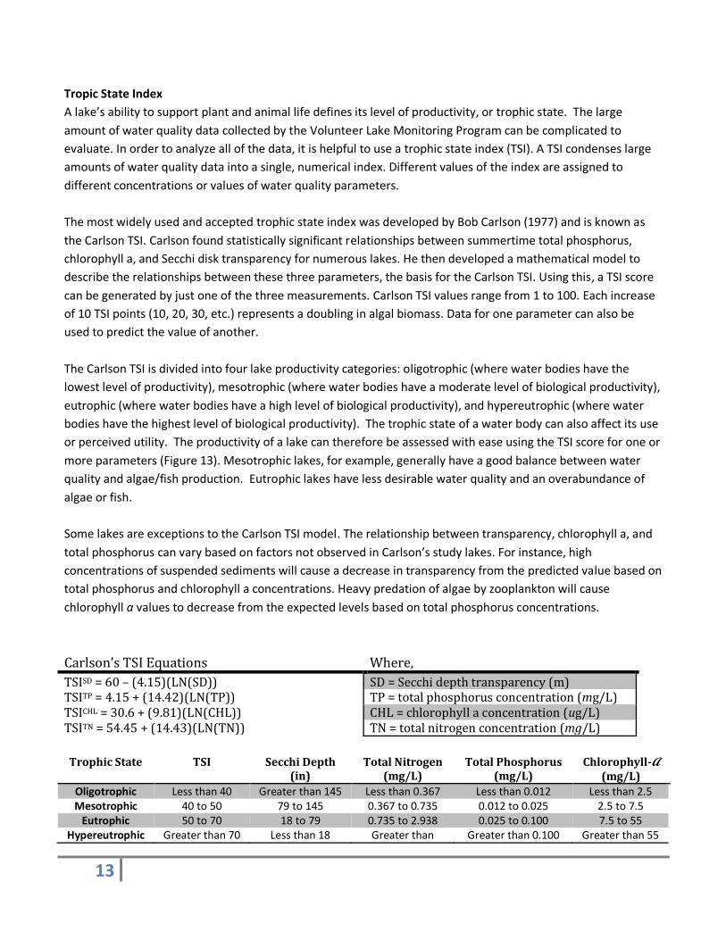
Carlson’s TSI Equations Where,
TSISD = 60 – (4.15)(LN(SD)) SD = Secchi depth transparency (m) TSITP = 4.15 + (14.42)(LN(TP)) TP = total phosphorus concentration (mg/L) TSICHL = 30.6 + (9.81)(LN(CHL)) CHL = chlorophyll a concentration (ug/L) TSITN = 54.45 + (14.43)(LN(TN)) TN = total nitrogen concentration (mg/L)
Trophic State TSI Secchi Depth (in)
Total Nitrogen (mg/L)
Total Phosphorus (mg/L)
Chlorophyll-A (mg/L)
Oligotrophic Less than 40 Greater than 145 Less than 0.367 Less than 0.012 Less than 2.5 Mesotrophic 40 to 50 79 to 145 0.367 to 0.735 0.012 to 0.025 2.5 to 7.5
Eutrophic 50 to 70 18 to 79 0.735 to 2.938 0.025 to 0.100 7.5 to 55 Hypereutrophic Greater than 70 Less than 18 Greater than Greater than 0.100 Greater than 55

14
2.938
A TSI based on average Secchi transparency for each lake is calculated to classify lakes according to their degree
of eutrophication as evidenced by their ability to support plant growth. As originally derived by Carlson, each
major division of the index (10, 20, 30, etc…) represents a theoretical doubling of plant productivity (algae
biomass). However, for Illinois lakes, the TSI value also reflects sediment-related turbidity; therefore, the higher
the TSI value, the greater impairment the lake likely exhibits from sediment-related turbidity and/or algal
growth. Lakes with an average Secchi transparency less than 79 inches (a TSI greater than 50) are classified as
eutrophic.
Using the Indices Beyond Classification
A major strength of TSI is that the interrelationships between variables can be used to identify certain conditions
in the lake or reservoir that are related to the factors that limit algal biomass or affect the measured variables.
When more than one of the three variables are measured, it is possible that different index values will be
obtained. Because the relationships between the variables were originally derived from regression relationships
and the correlations were not perfect, some variability between the index values is to be expected. However, in
some situations the variation is not random and factors interfering with the empirical relationship can be
identified. These deviations of the total phosphorus or the Secchi depth index from the chlorophyll index can be
used to identify errors in collection or analysis or real deviations from the “standard” expected values (Carlson
1981). Some possible interpretations of deviations of the index values are given in the table below (updated
from Carlson 1983).
Relationship Between TSI Variables Conditions
TSI(Chl) = TSI(TP) = TSI(SD) Algae dominate light attenuation; TN/TP ~ 33:1
TSI(Chl) > TSI(SD) Large particulates, such as Aphanizomenon flakes, dominate
TSI(TP) = TSI(SD) > TSI(CHL) Non-algal particulates or color dominate light attenuation
TSI(SD) = TSI(CHL) > TSI(TP) Phosphorus limits algal biomass (TN/TP >33:1)
TSI(TP) >TSI(CHL) = TSI(SD) Algae dominate light attenuation but some factor such as nitrogen limitation, zooplankton grazing or toxics limit algal biomass.
The simplest way to use the index for comparison of variables is to plot the seasonal trends of each of the
individual indices. If every TSI value for each variable is similar and tracks each other, then you know that the
lake is probably phosphorus limited (TN/TP = 33; Carlson 1992) and that most of the attenuation of light is by
algae.
In some lakes, the indices do not correspond throughout the season. In these cases, something very basic must
be affecting the relationships between the variables. The problem may be as simple as the data were calculated
incorrectly or that a measurement was done in a manner that produced different values. For example, if an
extractant other than acetone is used for chlorophyll analysis, a greater amount of chlorophyll might be
15
extracted from each cell, affecting the chlorophyll relationship with the other variables. If a volunteer incorrectly
measures Secchi depth, a systematic deviation might also occur.
After methodological errors can be ruled out, remaining systematic seasonal deviations may be caused by
interfering factors or non-measured limiting factors. Chlorophyll and Secchi depth indices might rise above the
phosphorus index, suggesting that the algae are becoming increasingly phosphorus limited. In other lakes or
during the season, the chlorophyll and transparency indices may be close together, but both will fall below the
phosphorus curve. This might suggest that the algae are nitrogen-limited or at least limited by some other factor
than phosphorus. Intense zooplankton grazing, for example, may cause the chlorophyll and Secchi depth indices
to fall below the phosphorus index as the zooplankton remove algal cells from the water or Secchi depth may
fall below chlorophyll if the grazers selectively eliminate the smaller cells.
In turbid lakes, it is common to see a close relationship between the total phosphorus TSI and the Secchi depth
TSI, while the chlorophyll index falls 10 or 20 units below the others. Clay particles contain phosphorus, and
therefore lakes with heavy clay turbidity will have the phosphorus correlated with the clay turbidity, while the
algae are neither able to utilize all the phosphorus nor contribute significantly to the light attenuation. This
relationship of the variables does not necessarily mean that the algae is limited by light, only that not all the
measured phosphorus is being utilized by the algae.
Finally, aquatic biomass productivity is affected by limiting certain nutrients, nitrogen and phosphorus. To apply
this method, the water body's limiting nutrient must be determined. The limiting nutrient is the nutrient of
lowest concentration that controls plant growth. This nutrient is normally phosphorus or nitrogen and in lakes it
is most often phosphorus.
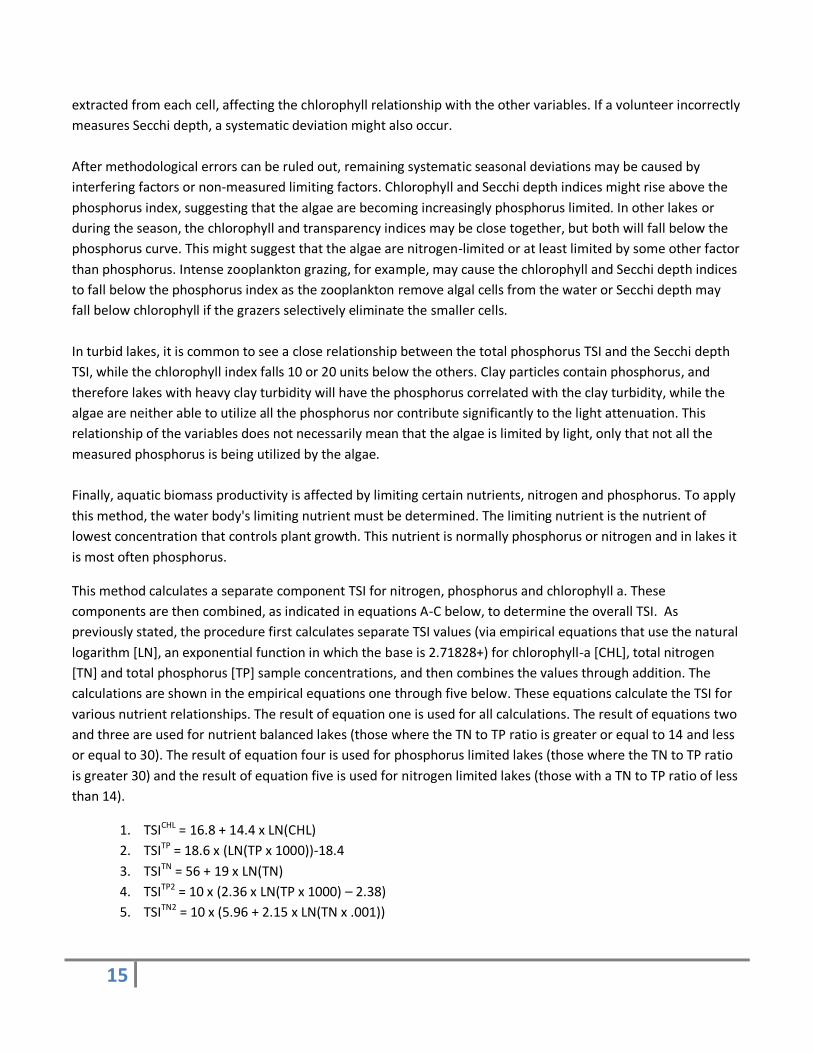
This method calculates a separate component TSI for nitrogen, phosphorus and chlorophyll a. These
components are then combined, as indicated in equations A-C below, to determine the overall TSI. As
previously stated, the procedure first calculates separate TSI values (via empirical equations that use the natural
logarithm [LN], an exponential function in which the base is 2.71828+) for chlorophyll-a [CHL], total nitrogen
[TN] and total phosphorus [TP] sample concentrations, and then combines the values through addition. The
calculations are shown in the empirical equations one through five below. These equations calculate the TSI for
various nutrient relationships. The result of equation one is used for all calculations. The result of equations two
and three are used for nutrient balanced lakes (those where the TN to TP ratio is greater or equal to 14 and less
or equal to 30). The result of equation four is used for phosphorus limited lakes (those where the TN to TP ratio
is greater 30) and the result of equation five is used for nitrogen limited lakes (those with a TN to TP ratio of less
than 14).
1. TSICHL = 16.8 + 14.4 x LN(CHL)
2. TSITP = 18.6 x (LN(TP x 1000))-18.4
3. TSITN = 56 + 19 x LN(TN)
4. TSITP2 = 10 x (2.36 x LN(TP x 1000) – 2.38)
5. TSITN2 = 10 x (5.96 + 2.15 x LN(TN x .001))
16
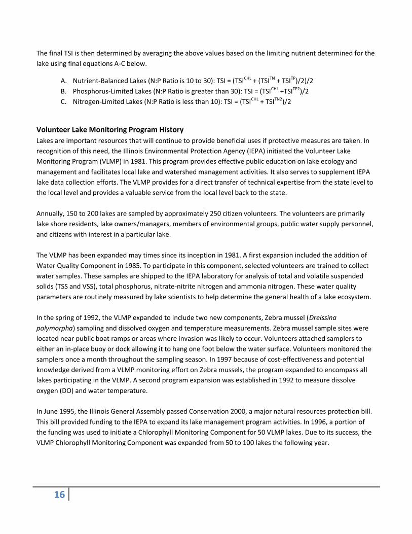
The final TSI is then determined by averaging the above values based on the limiting nutrient determined for the
lake using final equations A-C below.
A. Nutrient-Balanced Lakes (N:P Ratio is 10 to 30): TSI = (TSICHL + (TSITN + TSITP)/2)/2
B. Phosphorus-Limited Lakes (N:P Ratio is greater than 30): TSI = (TSICHL +TSITP2)/2
C. Nitrogen-Limited Lakes (N:P Ratio is less than 10): TSI = (TSICHL + TSITN2)/2
Volunteer Lake Monitoring Program History
Lakes are important resources that will continue to provide beneficial uses if protective measures are taken. In
recognition of this need, the Illinois Environmental Protection Agency (IEPA) initiated the Volunteer Lake
Monitoring Program (VLMP) in 1981. This program provides effective public education on lake ecology and
management and facilitates local lake and watershed management activities. It also serves to supplement IEPA
lake data collection efforts. The VLMP provides for a direct transfer of technical expertise from the state level to
the local level and provides a valuable service from the local level back to the state.
Annually, 150 to 200 lakes are sampled by approximately 250 citizen volunteers. The volunteers are primarily
lake shore residents, lake owners/managers, members of environmental groups, public water supply personnel,
and citizens with interest in a particular lake.
The VLMP has been expanded may times since its inception in 1981. A first expansion included the addition of
Water Quality Component in 1985. To participate in this component, selected volunteers are trained to collect
water samples. These samples are shipped to the IEPA laboratory for analysis of total and volatile suspended
solids (TSS and VSS), total phosphorus, nitrate-nitrite nitrogen and ammonia nitrogen. These water quality
parameters are routinely measured by lake scientists to help determine the general health of a lake ecosystem.
In the spring of 1992, the VLMP expanded to include two new components, Zebra mussel (Dreissina
polymorpha) sampling and dissolved oxygen and temperature measurements. Zebra mussel sample sites were
located near public boat ramps or areas where invasion was likely to occur. Volunteers attached samplers to
either an in-place buoy or dock allowing it to hang one foot below the water surface. Volunteers monitored the
samplers once a month throughout the sampling season. In 1997 because of cost-effectiveness and potential
knowledge derived from a VLMP monitoring effort on Zebra mussels, the program expanded to encompass all
lakes participating in the VLMP. A second program expansion was established in 1992 to measure dissolve
oxygen (DO) and water temperature.
In June 1995, the Illinois General Assembly passed Conservation 2000, a major natural resources protection bill.
This bill provided funding to the IEPA to expand its lake management program activities. In 1996, a portion of
the funding was used to initiate a Chlorophyll Monitoring Component for 50 VLMP lakes. Due to its success, the
VLMP Chlorophyll Monitoring Component was expanded from 50 to 100 lakes the following year.
17
Components of the VLMP
“Secchi Transparency”
Citizens select a lake to monitor and are then trained to measure water clarity (transparency) using a Secchi disk.
The Secchi disk was developed in 1865 by Professor P.A. Secchi for a Vatican-Financed Mediterranean
oceanographic expedition. At the time, it was used to determine if a ship could safely pass over a reef without
damaging its hull. It has since become a standard piece of equipment for lake scientists.
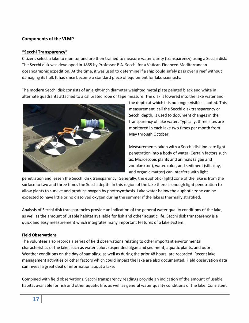
The modern Secchi disk consists of an eight-inch diameter weighted metal plate painted black and white in
alternate quadrants attached to a calibrated rope or tape measure. The disk is lowered into the lake water and
the depth at which it is no longer visible is noted. This
measurement, call the Secchi disk transparency or
Secchi depth, is used to document changes in the
transparency of lake water. Typically, three sites are
monitored in each lake two times per month from
May through October.
Measurements taken with a Secchi disk indicate light
penetration into a body of water. Certain factors such
as, Microscopic plants and animals (algae and
zooplankton), water color, and sediment (silt, clay,
and organic matter) can interfere with light
penetration and lessen the Secchi disk transparency. Generally, the euphotic (light) zone of the lake is from the
surface to two and three times the Secchi depth. In this region of the lake there is enough light penetration to
allow plants to survive and produce oxygen by photosynthesis. Lake water below the euphotic zone can be
expected to have little or no dissolved oxygen during the summer if the lake is thermally stratified.
Analysis of Secchi disk transparencies provide an indication of the general water quality conditions of the lake,
as well as the amount of usable habitat available for fish and other aquatic life. Secchi disk transparency is a
quick and easy measurement which integrates many important features of a lake system.
Field Observations
The volunteer also records a series of field observations relating to other important environmental
characteristics of the lake, such as water color, suspended algae and sediment, aquatic plants, and odor.
Weather conditions on the day of sampling, as well as during the prior 48 hours, are recorded. Recent lake
management activities or other factors which could impact the lake are also documented. Field observation data
can reveal a great deal of information about a lake.
Combined with field observations, Secchi transparency readings provide an indication of the amount of usable
habitat available for fish and other aquatic life, as well as general water quality conditions of the lake. Consistent
18
monitoring and observations throughout the sampling season and over a period of years can help identify lake
problems and causes, document water quality trends, and evaluate lake and watershed management strategies.
Aquatic Invasive Species
Aquatic invasive species (AIS) tracking has expanded over the years. AIS are freshwater organisms that spread or
are introduced outside their native habitats and cause negative environmental and/or economic impacts. You
also may hear AIS called aquatic “exotic,” “nuisance,” or “non-indigenous” species. Unfortunately, more than 85
AIS have been introduced into Illinois. The zebra mussel, Eurasian water milfoil, and silver carp are all examples
of invaders that have impacted our state.
Aquatic invaders such as these have been introduced and spread through a variety of activities including those
associated with recreational water users, backyard water gardeners, aquarium hobbyists, natural resource
professionals, the baitfish industry, and commercial shipping. The Illinois VLMP is partnering with Illinois-
Indiana Sea Grant, the Illinois Natural History Survey, and the Midwest Invasive Plant Network to monitor for
and help prevent the spread of aquatic invasive species to Illinois lakes.
Some of the AIS on the IEPA’s watch list include:
Mollusks: Zebra mussel, Quagga mussel, New Zealand mudsnail, Asian clam
Crustaceans: Rusty crayfish, Spiny water flea, Fishhook water flea, Bloody red shrimp
Fish: Round goby, Bighead & Silver carp (Asian carps), Ruffe, White perch
Aquatic Plants:
o Submersed (underwater) plants: Eurasian water milfoil, Curlyleaf pondweed, Brazilian elodea
(Brazilian waterweed), Hydrilla, Indian swampweed, Brittle waternymph (Brittle naiad)
o Free-floating plants: European frogbit, Water hyacinth, Water lettuce
o Rooted, floating-leaved plants: Pond water-starwort, Swamp stone crop, European waterclover,
Yellow floating heart, Water chestnut
o Emergent (above water) plants: Purple loosestrife, Flowering rush, Reed manna grass, Parrot
feather
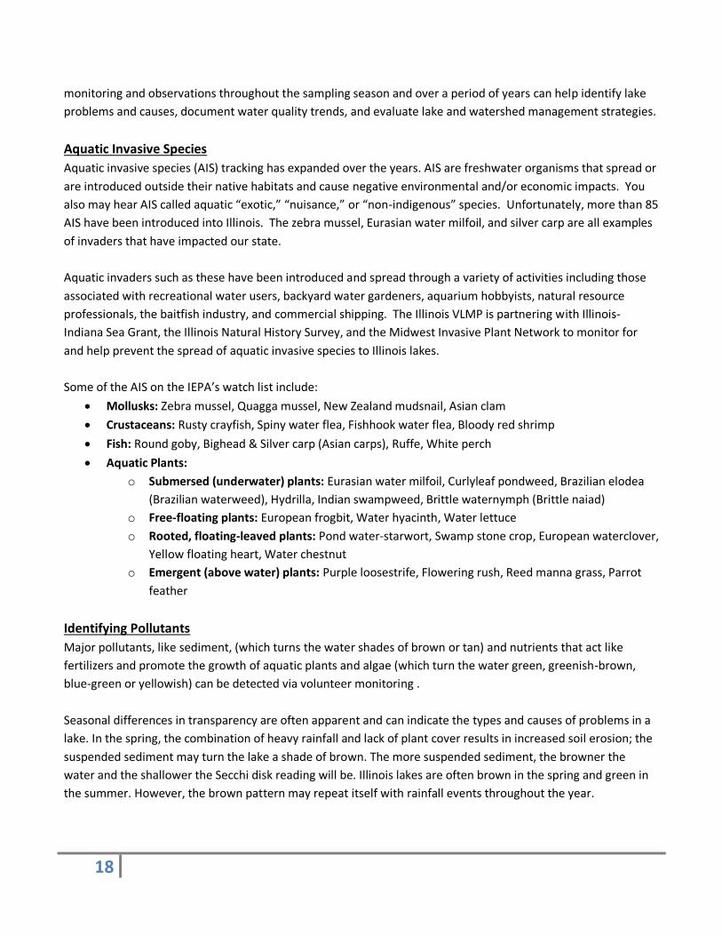
Identifying Pollutants
Major pollutants, like sediment, (which turns the water shades of brown or tan) and nutrients that act like
fertilizers and promote the growth of aquatic plants and algae (which turn the water green, greenish-brown,
blue-green or yellowish) can be detected via volunteer monitoring .
Seasonal differences in transparency are often apparent and can indicate the types and causes of problems in a
lake. In the spring, the combination of heavy rainfall and lack of plant cover results in increased soil erosion; the
suspended sediment may turn the lake a shade of brown. The more suspended sediment, the browner the
water and the shallower the Secchi disk reading will be. Illinois lakes are often brown in the spring and green in
the summer. However, the brown pattern may repeat itself with rainfall events throughout the year.
19
Deep lakes that have small amounts of incoming sediment from rainfall are generally clearer in the spring than
shallow lakes. They may remain relatively clear throughout the year or they may exhibit algal blooms. Lakes with
suspended sediment problems may show some improvement during the summer, when fewer storm events and
the development of crop cover in agricultural watersheds generally results in less soil erosion. These lakes, as
well as those that were relatively clear in the spring, may develop nuisance algal blooms during the summer if
excessive nutrients are present.
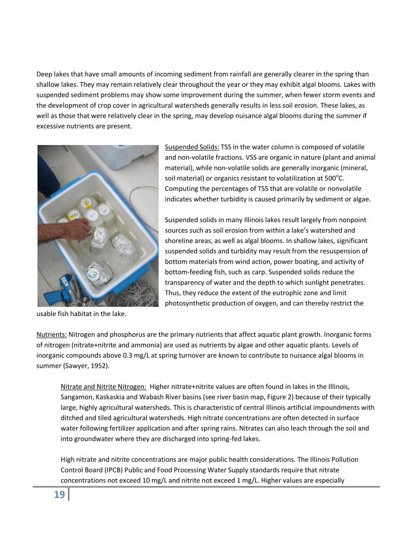
Suspended Solids: TSS in the water column is composed of volatile
and non-volatile fractions. VSS are organic in nature (plant and animal
material), while non-volatile solids are generally inorganic (mineral,
soil material) or organics resistant to volatilization at 500oC.
Computing the percentages of TSS that are volatile or nonvolatile
indicates whether turbidity is caused primarily by sediment or algae.
Suspended solids in many Illinois lakes result largely from nonpoint
sources such as soil erosion from within a lake’s watershed and
shoreline areas, as well as algal blooms. In shallow lakes, significant
suspended solids and turbidity may result from the resuspension of
bottom materials from wind action, power boating, and activity of
bottom-feeding fish, such as carp. Suspended solids reduce the
transparency of water and the depth to which sunlight penetrates.
Thus, they reduce the extent of the eutrophic zone and limit
photosynthetic production of oxygen, and can thereby restrict the
usable fish habitat in the lake.
Nutrients: Nitrogen and phosphorus are the primary nutrients that affect aquatic plant growth. Inorganic forms
of nitrogen (nitrate+nitrite and ammonia) are used as nutrients by algae and other aquatic plants. Levels of
inorganic compounds above 0.3 mg/L at spring turnover are known to contribute to nuisance algal blooms in
summer (Sawyer, 1952).
Nitrate and Nitrite Nitrogen: Higher nitrate+nitrite values are often found in lakes in the Illinois,
Sangamon, Kaskaskia and Wabash River basins (see river basin map, Figure 2) because of their typically
large, highly agricultural watersheds. This is characteristic of central Illinois artificial impoundments with
ditched and tiled agricultural watersheds. High nitrate concentrations are often detected in surface
water following fertilizer application and after spring rains. Nitrates can also leach through the soil and
into groundwater where they are discharged into spring-fed lakes.
High nitrate and nitrite concentrations are major public health considerations. The Illinois Pollution
Control Board (IPCB) Public and Food Processing Water Supply standards require that nitrate
concentrations not exceed 10 mg/L and nitrite not exceed 1 mg/L. Higher values are especially
20
dangerous to infants less than six months old because of their susceptibility to methemoglobinemia,
“blue baby syndrome.”
Total Ammonia Nitrogen: Ammonia in fresh water can be extremely toxic to aquatic organisms, while at
the same time it is a source of nutrients that promote plant growth. For “General Use” waters, the IPCB
specifies that total ammonia nitrogen shall not exceed 15 mg/L, and un-ionized ammonia shall not
exceed 0.04 mg/L. Ammonia nitrogen in aquatic systems usually occurs in high(er) concentrations only
when dissolved oxygen is low or depleted.
Phosphorus: Phosphorus is an essential nutrient for plant and animal growth. It is a constituent of
fertile soils, plants, and protoplasm. It also plays a vital role in energy transfer during cell metabolism. To
restrict noxious growth of algae and other aquatic plants, the IPCB established a General Use standard
of 0.05 mg/L for total phosphorus (TP) in any lake, or in any stream at the point where it enters a lake.
Allum et al (1977) classified oligotrophic lakes as those with TP values below 0.01 mg/L and mesotrophic
as those lakes with TP values between 0.01 and 0.02 mg/L. Eutrophic lakes have TP values greater than
0.02 mg/L.
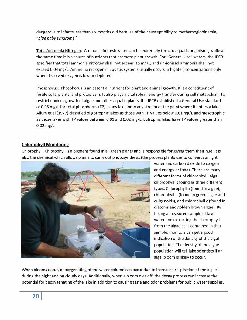
Chlorophyll Monitoring
Chlorophyll: Chlorophyll is a pigment found in all green plants and is responsible for giving them their hue. It is
also the chemical which allows plants to carry out photosynthesis (the process plants use to convert sunlight,
water and carbon dioxide to oxygen
and energy or food). There are many
different forms of chlorophyll. Algal
chlorophyll is found as three different
types. Chlorophyll a (found in algae),
chlorophyll b (found in green algae and
eulgenoids), and chlorophyll c (found in
diatoms and golden brown algae). By
taking a measured sample of lake
water and extracting the chlorophyll
from the algae cells contained in that
sample, monitors can get a good
indication of the density of the algal
population. The density of the algae
population will tell lake scientists if an
algal bloom is likely to occur.
When blooms occur, deoxygenating of the water column can occur due to increased respiration of the algae
during the night and on cloudy days. Additionally, when a bloom dies off, the decay process can increase the
potential for deoxygenating of the lake in addition to causing taste and odor problems for public water supplies.

21
The chlorophyll sample is taken at twice the Secchi depth and is filtered by the volunteer. The water quality
sample and the chlorophyll samples are then mailed to the IEPA’s Springfield laboratory for analysis. All training,
equipment, and analysis are free of charge to the volunteers.
Dissolved Oxygen/Temperature
These two water quality measurements play important roles in the overall health of lakes. Most living organisms
need oxygen to survive. So it is important to know how much and at what depth dissolved oxygen is available to
these organisms. Low oxygen levels often occur during summer and winter stratification. During the summer in
Illinois’ stratified mesotrophic lakes, the top layer is warm, highly oxygenated water (epilimnion), while the
bottom waters are very low in oxygen and much cooler (hypolimnion).
Oxygen can enter the water column in several ways. The most
common are through photosynthesis of aquatic plants and
algae, as well as through diffusion of oxygen entering the lake
from the atmosphere. Oxygen can also enter the lake via water
from inflowing tributaries.
The amount of oxygen that can be dissolved in water is
determined by the water’s temperature. Cooler water can hold
more oxygen than warmer water. Often, the amount of oxygen
in water is reported as percent saturation. During an algal
bloom, the algae can put more oxygen into the water than the
water can normally hold; this is called super-saturation. The percent saturation is calculated as a ratio of the
lake’s actual DO concentration and the maximum concentration possible under saturated conditions. During an
algal bloom, the percent saturation may exceed 200 percent. Conversely, the mass dying of algae and/or
macrophytes can cause a depletion of DO as
organisms that use oxygen feed on dead
material.
SUPER-SATURATION AND DEPLETION GRAPH
(Wetzel 2001)
The graph depicts the dramatic difference
between a nutritionally balanced lake and a
eutrophic lake. Depending on fish species,
dissolved oxygen dropping below a certain
threshold may cause a “fish kill.”
22
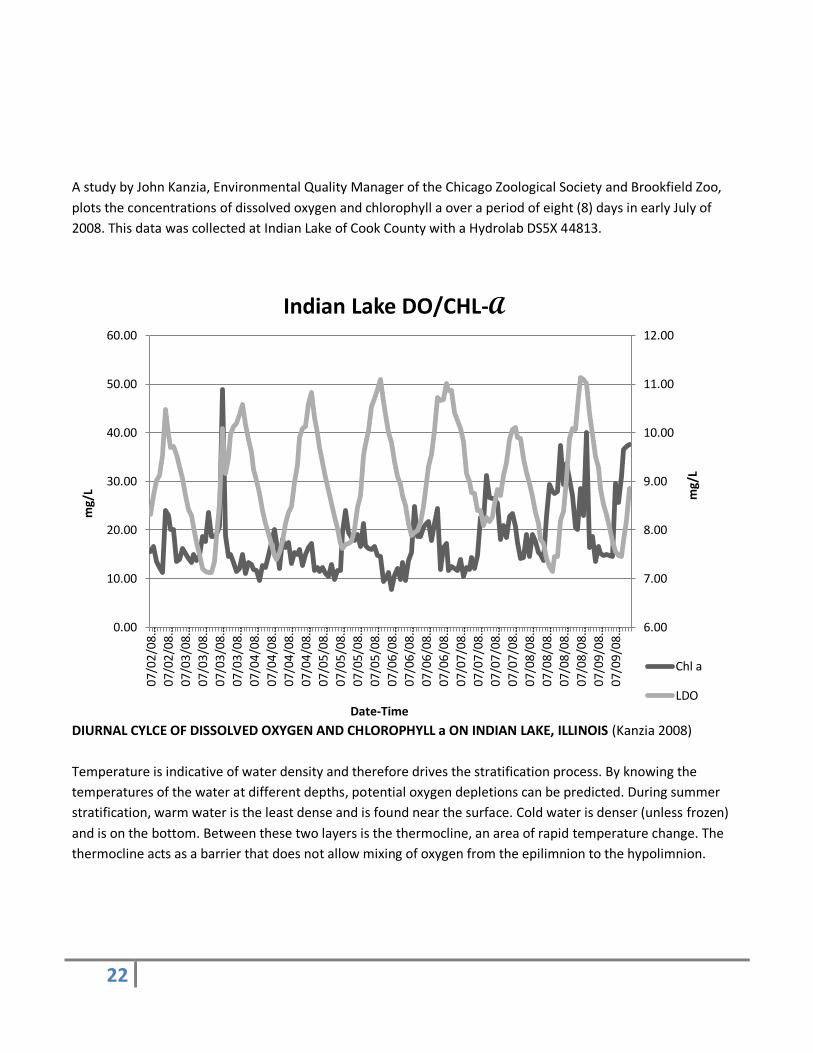
A study by John Kanzia, Environmental Quality Manager of the Chicago Zoological Society and Brookfield Zoo,
plots the concentrations of dissolved oxygen and chlorophyll a over a period of eight (8) days in early July of
2008. This data was collected at Indian Lake of Cook County with a Hydrolab DS5X 44813.
DIURNAL CYLCE OF DISSOLVED OXYGEN AND CHLOROPHYLL a ON INDIAN LAKE, ILLINOIS (Kanzia 2008)
Temperature is indicative of water density and therefore drives the stratification process. By knowing the
temperatures of the water at different depths, potential oxygen depletions can be predicted. During summer
stratification, warm water is the least dense and is found near the surface. Cold water is denser (unless frozen)
and is on the bottom. Between these two layers is the thermocline, an area of rapid temperature change. The
thermocline acts as a barrier that does not allow mixing of oxygen from the epilimnion to the hypolimnion.
6.00
7.00
8.00
9.00
10.00
11.00
12.00
0.00
10.00
20.00
30.00
40.00
50.00
60.00
07/0
2/0
8…
07/0
2/0
8…
07/0
3/0
8…
07/0
3/0
8…
07/0
3/0
8…
07/0
3/0
8…
07/0
4/0
8…
07/0
4/0
8…
07/0
4/0
8…
07/0
4/0
8…
07/0
5/0
8…
07/0
5/0
8…
07/0
5/0
8…
07/0
5/0
8…
07/0
6/0
8…
07/0
6/0
8…
07/0
6/0
8…
07/0
6/0
8…
07/0
7/0
8…
07/0
7/0
8…
07/0
7/0
8…
07/0
7/0
8…
07/0
8/0
8…
07/0
8/0
8…
07/0
8/0
8…
07/0
8/0
8…
07/0
9/0
8…
07/0
9/0
8…
mg/
L
mg/
L
Date-Time
Indian Lake DO/CHL-A
Chl a
LDO
23
Methods and Procedures
Volunteer Recognition and Education
At the beginning of the season, new volunteers were presented cloth emblems to display on clothing
highlighting their involvement in the VLMP. At the end of the sampling season, all volunteers who monitored
four or more sampling periods were sent a Certificate of Appreciation.
As another way to honor volunteers each year, a session at the Illinois Lake Management Association’s Annual
Conference is designated as the Volunteer Lake Monitoring Program Session. Outstanding VLMP volunteers are
presented with plaques and lapel pins to commemorate years of service. Session participants also receive
information about other volunteer programs and an update on the VLMP for the upcoming sampling season.
Volunteers also receive a VLMP newsletter. These
newsletters contain reminders for the volunteers regarding
VLMP, as well as educational information on lake conditions,
management, and monitoring.
Training Volunteers
Training of new volunteers, “refresher” training for returning
volunteers and expanded monitoring training was conducted
by staff coordinators from IEPA’s Lake Program, as well as
from Regional Coordinators. In all cases, this training took
place at the volunteer’s lake. During the training sessions, the
coordinator used the volunteer’s boat to visit each sampling
site, whereupon the volunteer was instructed in the proper
sampling procedures.
Basic Monitoring Program
Volunteers typically take lake water transparency readings
with a Secchi disk at three designated sites, generally twice a
month from May 1 through October 31. The sites are chosen
after a review of the lake’s physical statistics including a
bathymetric map, location and size of inlets and outlets, and
any structures or features affecting the lake, such as, farms,
residential properties, commercial or industrial properties and
old dam or infrastructure with the confines of the lake bed.
Site one is typically the deepest part of the lake. In
impoundment lakes, that is most often near the dam.
Two or more additional sites are identified in the inlets
(fingers) for the lake, in channels deep enough for volunteers to reach by boat. A site map is generated by the
24
program personnel that includes the general site locations, Global Positioning System (GPS) coordinates (if
available), and a unique site code identifying the lake.
Basic Monitoring Procedures
The volunteer proceeds to a site using a lake map. The order for monitoring the lake sites is not specific.
Locations are located specifically by either using “sight lines” (aligning 2 sets of landmarks on shore) or by GPS
coordinates. After reaching the monitoring site, the volunteer carefully lowers the anchor over the side of the
boat until it reaches the lake bottom, letting out plenty of anchor line so that the boat drifts away from any
sediment disturbed by the anchor.
The volunteer must remove any sunglasses, hat or object which may obstruct a clear view of the Secchi disk. The
Secchi disk is then slowly lowered into the water until it can no longer be seen. At the point where the volunteer
lose sight of the disk, the rope or survey tape is marked at the water level with a clothespin. The Secchi disk is
then lowered about 1 to 2 more feet into the water, before slowly being raised towards the water surface.
When the disk reappears, the line is again marked by pinching the rope or survey tape at the water level with
the fingers. The rope/survey tape and Secchi disk are brought back into the boat, being careful not to release
your “pinching” fingers. A loop is formed between the clothespin and the pinching fingers, sliding the clothespin
to the center (the top) of the loop. This marks the average of the two transparency readings. The number of
inches between the disk and the clothespin, to the closest inch, is recorded on the Secchi Monitoring Form,
along with the time (in 24-hour format) that the measurement was taken.
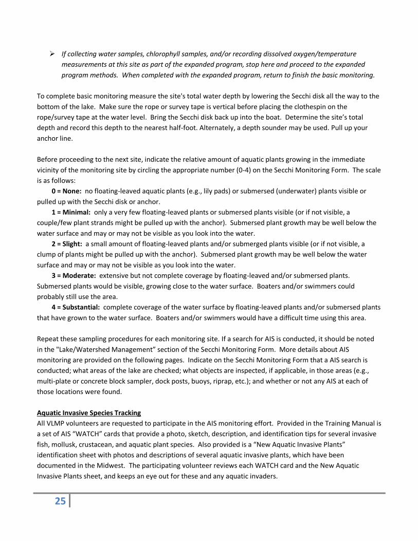
Sometimes, the "true" Secchi disk transparency can't be measured
because either: the disk reached the lake bottom and could still be
seen or the disk was lost from view because it "disappeared" into
dense growth of rooted aquatic plants. Sometimes moving a few
feet will permit the Secchi disk to be observed through the aquatic
plants, however, this situation cannot always be avoided. The
Secchi Monitoring Form is annotated to reflect these two potential
situations. Secchi disk transparency reading is recorded regardless
of these situations.
Volunteers also record apparent water color at each location. Determine the water color by lowering the Secchi
disk (on the shaded side of the boat) to one-half (½) the Secchi transparency. Holding the Color Chart just above
the surface of the water near one of the disk's white quadrants, compare the color of the white quadrant with
the various colors on the standardized color chart, and record the corresponding number on the Secchi
Monitoring Form. If no exact match exists, record the color number that is the closest match or a 20 to
represent “other.” If choosing other, please provide your observations in “Additional Observations.” If the
Secchi transparency was limited by either reaching the lake bed or plant growth, do not take a color reading
(just place a dash or "n/a" for color on the Secchi Monitoring Form).
25
If collecting water samples, chlorophyll samples, and/or recording dissolved oxygen/temperature
measurements at this site as part of the expanded program, stop here and proceed to the expanded
program methods. When completed with the expanded program, return to finish the basic monitoring.
To complete basic monitoring measure the site's total water depth by lowering the Secchi disk all the way to the
bottom of the lake. Make sure the rope or survey tape is vertical before placing the clothespin on the
rope/survey tape at the water level. Bring the Secchi disk back up into the boat. Determine the site’s total
depth and record this depth to the nearest half-foot. Alternately, a depth sounder may be used. Pull up your
anchor line.
Before proceeding to the next site, indicate the relative amount of aquatic plants growing in the immediate
vicinity of the monitoring site by circling the appropriate number (0-4) on the Secchi Monitoring Form. The scale
is as follows:
0 = None: no floating-leaved aquatic plants (e.g., lily pads) or submersed (underwater) plants visible or
pulled up with the Secchi disk or anchor.
1 = Minimal: only a very few floating-leaved plants or submersed plants visible (or if not visible, a
couple/few plant strands might be pulled up with the anchor). Submersed plant growth may be well below the
water surface and may or may not be visible as you look into the water.
2 = Slight: a small amount of floating-leaved plants and/or submerged plants visible (or if not visible, a
clump of plants might be pulled up with the anchor). Submersed plant growth may be well below the water
surface and may or may not be visible as you look into the water.
3 = Moderate: extensive but not complete coverage by floating-leaved and/or submersed plants.
Submersed plants would be visible, growing close to the water surface. Boaters and/or swimmers could
probably still use the area.
4 = Substantial: complete coverage of the water surface by floating-leaved plants and/or submersed plants
that have grown to the water surface. Boaters and/or swimmers would have a difficult time using this area.
Repeat these sampling procedures for each monitoring site. If a search for AIS is conducted, it should be noted
in the "Lake/Watershed Management” section of the Secchi Monitoring Form. More details about AIS
monitoring are provided on the following pages. Indicate on the Secchi Monitoring Form that a AIS search is
conducted; what areas of the lake are checked; what objects are inspected, if applicable, in those areas (e.g.,
multi-plate or concrete block sampler, dock posts, buoys, riprap, etc.); and whether or not any AIS at each of
those locations were found.
Aquatic Invasive Species Tracking
All VLMP volunteers are requested to participate in the AIS monitoring effort. Provided in the Training Manual is
a set of AIS “WATCH” cards that provide a photo, sketch, description, and identification tips for several invasive
fish, mollusk, crustacean, and aquatic plant species. Also provided is a “New Aquatic Invasive Plants”
identification sheet with photos and descriptions of several aquatic invasive plants, which have been
documented in the Midwest. The participating volunteer reviews each WATCH card and the New Aquatic
Invasive Plants sheet, and keeps an eye out for these and any aquatic invaders.
26
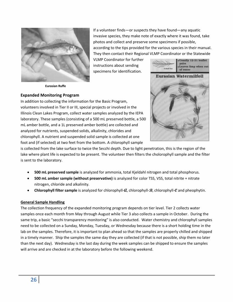
If a volunteer finds—or suspects they have found—any aquatic
invasive species, they make note of exactly where it was found, take
photos and collect and preserve some specimens if possible,
according to the tips provided for the various species in their manual.
They then contact their Regional VLMP Coordinator or the Statewide
VLMP Coordinator for further
instructions about sending
specimens for identification.
Expanded Monitoring Program
In addition to collecting the information for the Basic Program,
volunteers involved in Tier II or III, special projects or involved in the
Illinois Clean Lakes Program, collect water samples analyzed by the IEPA
laboratory. These samples (consisting of a 500 mL preserved bottle, a 500
mL amber bottle, and a 1L preserved amber bottle) are collected and
analyzed for nutrients, suspended solids, alkalinity, chlorides and
chlorophyll. A nutrient and suspended solid sample is collected at one
foot and (if selected) at two feet from the bottom. A chlorophyll sample
is collected from the lake surface to twice the Secchi depth. Due to light penetration, this is the region of the
lake where plant life is expected to be present. The volunteer then filters the cholorophyll sample and the filter
is sent to the laboratory.
500 mL preserved sample is analyzed for ammonia, total Kjeldahl nitrogen and total phosphorus.
500 mL amber sample (without preservative) is analyzed for color TSS, VSS, total nitrite + nitrate
nitrogen, chloride and alkalinity.
Chlorophyll filter sample is analyzed for chlorophyll-A, chlorophyll-B, chlorophyll-C and pheophytin.
General Sample Handling
The collection frequency of the expanded monitoring program depends on tier level. Tier 2 collects water
samples once each month from May through August while Tier 3 also collects a sample in October. During the
same trip, a basic “secchi transparency monitoring” is also conducted. Water chemistry and chlorophyll samples
need to be collected on a Sunday, Monday, Tuesday, or Wednesday because there is a short holding time in the
lab on the samples. Therefore, it is important to plan ahead so that the samples are properly chilled and shipped
in a timely manner. Ship the samples the same day they are collected (if that is not possible, ship them no later
than the next day). Wednesday is the last day during the week samples can be shipped to ensure the samples
will arrive and are checked in at the laboratory before the following weekend.
Eurasian Ruffe
27
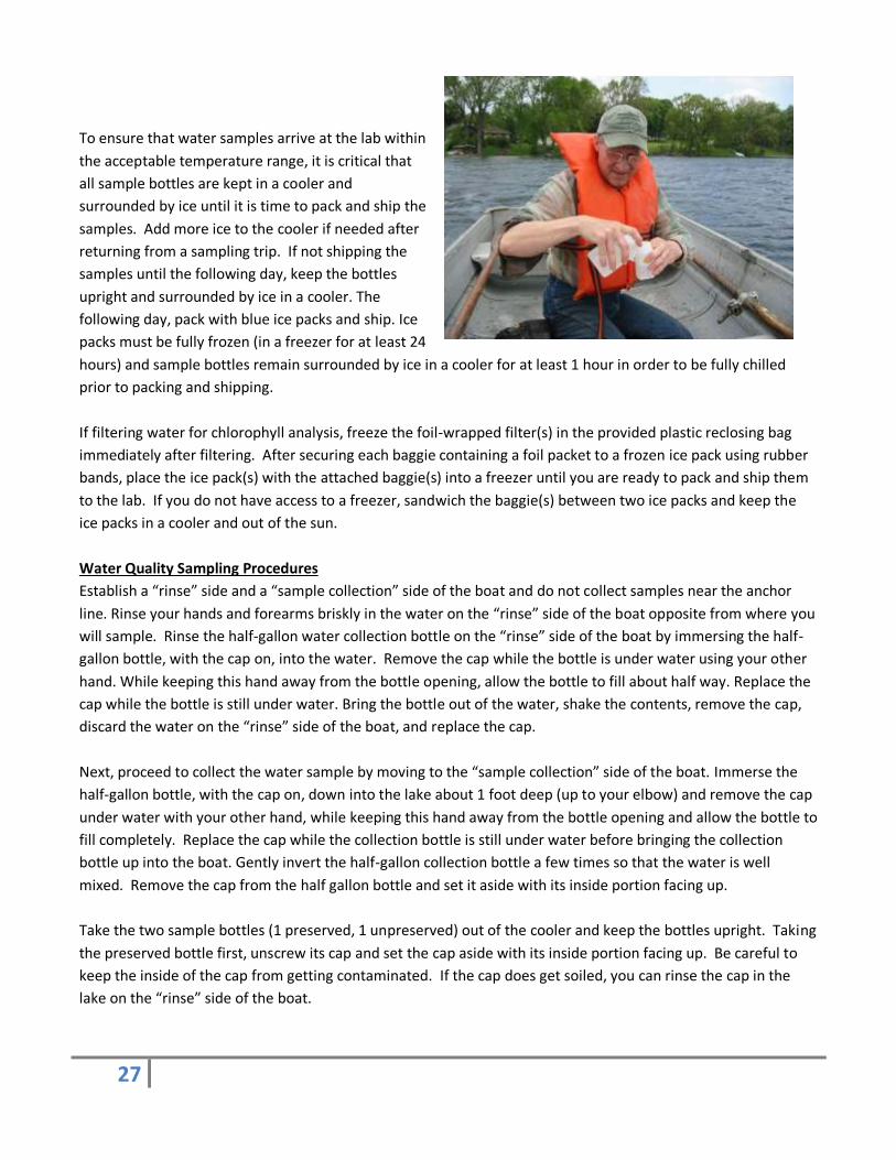
To ensure that water samples arrive at the lab within
the acceptable temperature range, it is critical that
all sample bottles are kept in a cooler and
surrounded by ice until it is time to pack and ship the
samples. Add more ice to the cooler if needed after
returning from a sampling trip. If not shipping the
samples until the following day, keep the bottles
upright and surrounded by ice in a cooler. The
following day, pack with blue ice packs and ship. Ice
packs must be fully frozen (in a freezer for at least 24
hours) and sample bottles remain surrounded by ice in a cooler for at least 1 hour in order to be fully chilled
prior to packing and shipping.
If filtering water for chlorophyll analysis, freeze the foil-wrapped filter(s) in the provided plastic reclosing bag
immediately after filtering. After securing each baggie containing a foil packet to a frozen ice pack using rubber
bands, place the ice pack(s) with the attached baggie(s) into a freezer until you are ready to pack and ship them
to the lab. If you do not have access to a freezer, sandwich the baggie(s) between two ice packs and keep the
ice packs in a cooler and out of the sun.
Water Quality Sampling Procedures
Establish a “rinse” side and a “sample collection” side of the boat and do not collect samples near the anchor
line. Rinse your hands and forearms briskly in the water on the “rinse” side of the boat opposite from where you
will sample. Rinse the half-gallon water collection bottle on the “rinse” side of the boat by immersing the half-
gallon bottle, with the cap on, into the water. Remove the cap while the bottle is under water using your other
hand. While keeping this hand away from the bottle opening, allow the bottle to fill about half way. Replace the
cap while the bottle is still under water. Bring the bottle out of the water, shake the contents, remove the cap,
discard the water on the “rinse” side of the boat, and replace the cap.
Next, proceed to collect the water sample by moving to the “sample collection” side of the boat. Immerse the
half-gallon bottle, with the cap on, down into the lake about 1 foot deep (up to your elbow) and remove the cap
under water with your other hand, while keeping this hand away from the bottle opening and allow the bottle to
fill completely. Replace the cap while the collection bottle is still under water before bringing the collection
bottle up into the boat. Gently invert the half-gallon collection bottle a few times so that the water is well
mixed. Remove the cap from the half gallon bottle and set it aside with its inside portion facing up.
Take the two sample bottles (1 preserved, 1 unpreserved) out of the cooler and keep the bottles upright. Taking
the preserved bottle first, unscrew its cap and set the cap aside with its inside portion facing up. Be careful to
keep the inside of the cap from getting contaminated. If the cap does get soiled, you can rinse the cap in the
lake on the “rinse” side of the boat.
28
Slowly pour the water from the half-gallon collection bottle into the preserved sample bottle. Fill the sample
bottle to just under its shoulder. Be careful not to overfill the preserved bottle, since it
contains an acid preservative. Recap the preserved sample bottle tightly and gently
rotate and invert the sample bottle to ensure the preservative is well-mixed with the
sample water. Then follow the same procedure to fill the unpreserved sample bottle.
Both the preserved and unpreserved sample bottles must be filled from the same half-
gallon water collection.
If you overfill the preserved bottle, mark a big “X” across its label and set it aside for
later disposal. Write the appropriate SAMPLE ID on a new preserved bottle. Pour out
the lake water that’s still in the half-gallon collection bottle on the “rinse” side of the
boat, then resample as described above.
Immediately place the two sample bottles into a cooler with ice. Push the bottles into
the ice so they are upright and surrounded by ice. Remember to close the lid, so
sunlight cannot reach the samples. Discard any remaining water in the half-gallon
collection bottle on the “rinse” side of the boat.
Chlorophyll Sampling Procedures
Check the water depth again using the handheld depth sounder. The chlorophyll
sampling depth is twice the Secchi transparency, to the nearest foot, unless the lake is
not deep enough at the monitoring site or if aquatic plants might interfere with
sample collection. In these cases, the depth is reduced to 2 feet from the bottom of
the lake or to a depth that does not touch plant growth. In all cases, collect the
chlorophyll sample to the nearest foot. Also make sure to record the chlorophyll
sample collection depth on the Secchi Monitoring Form and chlorophyll lab sheet.
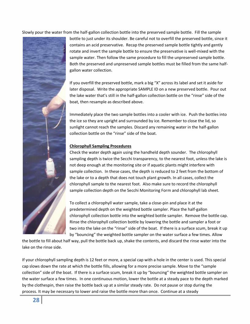
To collect a chlorophyll water sample, take a close-pin and place it at the
predetermined depth on the weighted bottle sampler. Place the half-gallon
chlorophyll collection bottle into the weighted bottle sampler. Remove the bottle cap.
Rinse the chlorophyll collection bottle by lowering the bottle and sampler a foot or
two into the lake on the “rinse” side of the boat. If there is a surface scum, break it up
by “bouncing” the weighted bottle sampler on the water surface a few times. Allow
the bottle to fill about half way, pull the bottle back up, shake the contents, and discard the rinse water into the
lake on the rinse side.
If your chlorophyll sampling depth is 12 feet or more, a special cap with a hole in the center is used. This special
cap slows down the rate at which the bottle fills, allowing for a more precise sample. Move to the “sample
collection” side of the boat. If there is a surface scum, break it up by “bouncing” the weighted bottle sampler on
the water surface a few times. In one continuous motion, lower the bottle at a steady pace to the depth marked
by the clothespin, then raise the bottle back up at a similar steady rate. Do not pause or stop during the
process. It may be necessary to lower and raise the bottle more than once. Continue at a steady
29
lowering/raising pace until the bottle is one-half (1/2) to two-thirds (2/3) full. If the collection bottle is
completely (or even nearly completely) full after you pull it up, you must discard the water on the “rinse” side of
the boat and start over. As you lower and raise the weighted bottle sampler, never let it touch the lake bottom
or rub against aquatic plants. Bring the weighted bottle sampler into the boat. Place the solid cap on the half-
gallon bottle and tighten, then remove the bottle from the sampler. Gently invert the half-gallon bottle several
times to ensure the water is well mixed.
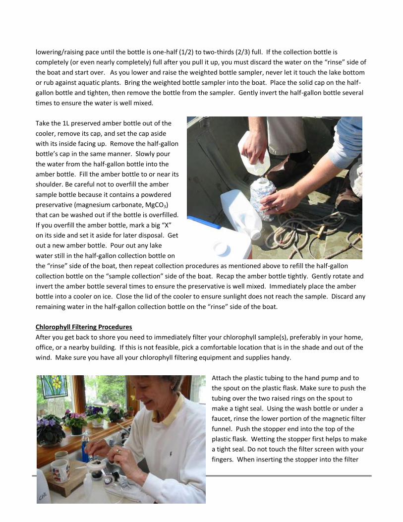
Take the 1L preserved amber bottle out of the
cooler, remove its cap, and set the cap aside
with its inside facing up. Remove the half-gallon
bottle’s cap in the same manner. Slowly pour
the water from the half-gallon bottle into the
amber bottle. Fill the amber bottle to or near its
shoulder. Be careful not to overfill the amber
sample bottle because it contains a powdered
preservative (magnesium carbonate, MgCO3)
that can be washed out if the bottle is overfilled.
If you overfill the amber bottle, mark a big “X”
on its side and set it aside for later disposal. Get
out a new amber bottle. Pour out any lake
water still in the half-gallon collection bottle on
the “rinse” side of the boat, then repeat collection procedures as mentioned above to refill the half-gallon
collection bottle on the “sample collection” side of the boat. Recap the amber bottle tightly. Gently rotate and
invert the amber bottle several times to ensure the preservative is well mixed. Immediately place the amber
bottle into a cooler on ice. Close the lid of the cooler to ensure sunlight does not reach the sample. Discard any
remaining water in the half-gallon collection bottle on the “rinse” side of the boat.
Chlorophyll Filtering Procedures
After you get back to shore you need to immediately filter your chlorophyll sample(s), preferably in your home,
office, or a nearby building. If this is not feasible, pick a comfortable location that is in the shade and out of the
wind. Make sure you have all your chlorophyll filtering equipment and supplies handy.
Attach the plastic tubing to the hand pump and to
the spout on the plastic flask. Make sure to push the
tubing over the two raised rings on the spout to
make a tight seal. Using the wash bottle or under a
faucet, rinse the lower portion of the magnetic filter
funnel. Push the stopper end into the top of the
plastic flask. Wetting the stopper first helps to make
a tight seal. Do not touch the filter screen with your
fingers. When inserting the stopper into the filter
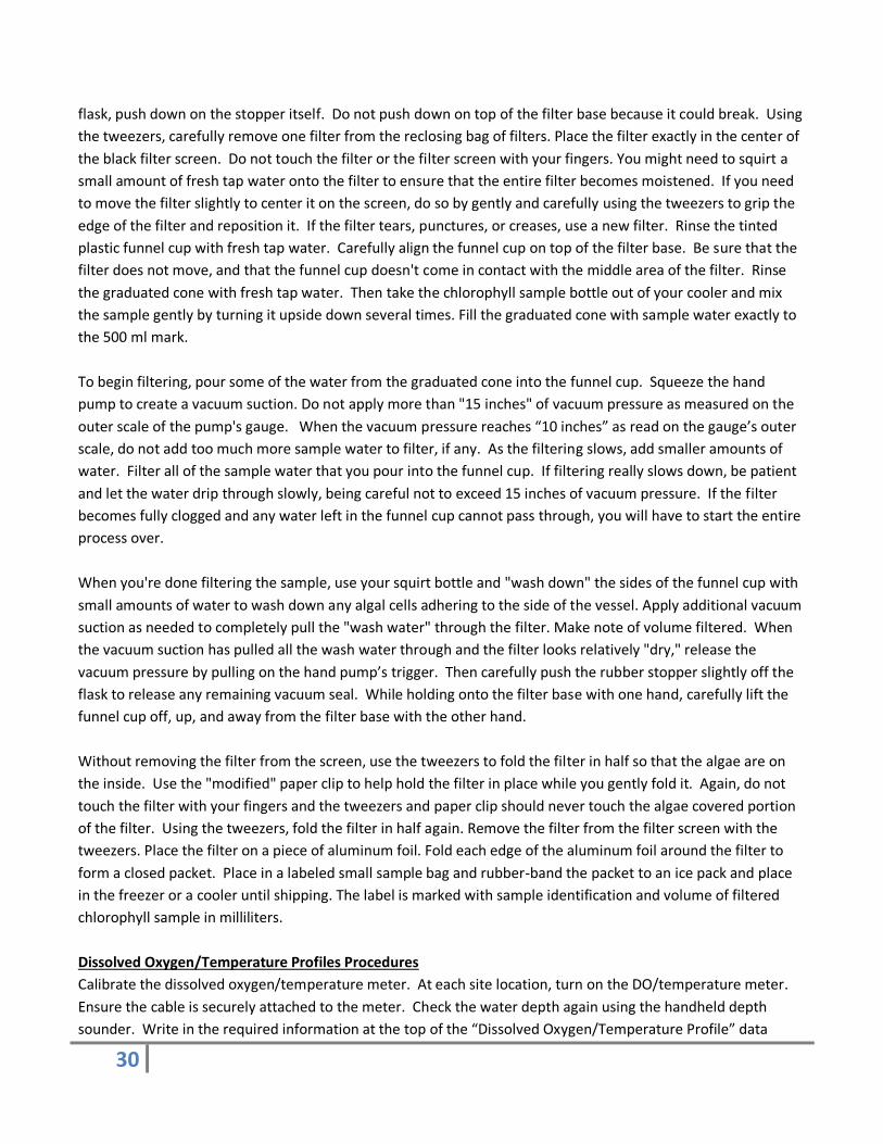
30
flask, push down on the stopper itself. Do not push down on top of the filter base because it could break. Using
the tweezers, carefully remove one filter from the reclosing bag of filters. Place the filter exactly in the center of
the black filter screen. Do not touch the filter or the filter screen with your fingers. You might need to squirt a
small amount of fresh tap water onto the filter to ensure that the entire filter becomes moistened. If you need
to move the filter slightly to center it on the screen, do so by gently and carefully using the tweezers to grip the
edge of the filter and reposition it. If the filter tears, punctures, or creases, use a new filter. Rinse the tinted
plastic funnel cup with fresh tap water. Carefully align the funnel cup on top of the filter base. Be sure that the
filter does not move, and that the funnel cup doesn't come in contact with the middle area of the filter. Rinse
the graduated cone with fresh tap water. Then take the chlorophyll sample bottle out of your cooler and mix
the sample gently by turning it upside down several times. Fill the graduated cone with sample water exactly to
the 500 ml mark.
To begin filtering, pour some of the water from the graduated cone into the funnel cup. Squeeze the hand
pump to create a vacuum suction. Do not apply more than "15 inches" of vacuum pressure as measured on the
outer scale of the pump's gauge. When the vacuum pressure reaches “10 inches” as read on the gauge’s outer
scale, do not add too much more sample water to filter, if any. As the filtering slows, add smaller amounts of
water. Filter all of the sample water that you pour into the funnel cup. If filtering really slows down, be patient
and let the water drip through slowly, being careful not to exceed 15 inches of vacuum pressure. If the filter
becomes fully clogged and any water left in the funnel cup cannot pass through, you will have to start the entire
process over.
When you're done filtering the sample, use your squirt bottle and "wash down" the sides of the funnel cup with
small amounts of water to wash down any algal cells adhering to the side of the vessel. Apply additional vacuum
suction as needed to completely pull the "wash water" through the filter. Make note of volume filtered. When
the vacuum suction has pulled all the wash water through and the filter looks relatively "dry," release the
vacuum pressure by pulling on the hand pump’s trigger. Then carefully push the rubber stopper slightly off the
flask to release any remaining vacuum seal. While holding onto the filter base with one hand, carefully lift the
funnel cup off, up, and away from the filter base with the other hand.
Without removing the filter from the screen, use the tweezers to fold the filter in half so that the algae are on
the inside. Use the "modified" paper clip to help hold the filter in place while you gently fold it. Again, do not
touch the filter with your fingers and the tweezers and paper clip should never touch the algae covered portion
of the filter. Using the tweezers, fold the filter in half again. Remove the filter from the filter screen with the
tweezers. Place the filter on a piece of aluminum foil. Fold each edge of the aluminum foil around the filter to
form a closed packet. Place in a labeled small sample bag and rubber-band the packet to an ice pack and place
in the freezer or a cooler until shipping. The label is marked with sample identification and volume of filtered
chlorophyll sample in milliliters.
Dissolved Oxygen/Temperature Profiles Procedures
Calibrate the dissolved oxygen/temperature meter. At each site location, turn on the DO/temperature meter.
Ensure the cable is securely attached to the meter. Check the water depth again using the handheld depth
sounder. Write in the required information at the top of the “Dissolved Oxygen/Temperature Profile” data
31
form: unique station code, lake name and county, volunteer name(s), date (mm/dd/yyyy), time (hh:mm), meter
brand/model (e.g., Hach HQ30d, Hydrolab Quanta, YSI 550A), IEPA case/meter #, barometer reading, and
comments. Fill in each depth (in whole numbers) in the left column of the data form, down to 2 feet above the
lake bottom The “0” and “1” foot depths have been pre-printed on the form.
Place the probe into the lake. Make sure the tip of the probe is under the water surface by immersing the probe
to the top of the protective shroud’s locking ring. (This is the “0” depth.) Press the “Read” button. When the
display indicates a stabilized reading when the meter beeps and a padlock icon appears in the upper left corner
of the screen. Record the displayed DO and temperature readings on the data form, rounding to the nearest
tenth. The DO is displayed in mg/L (milligrams per liter), and the temperature is in °C (degrees Celsius).
Repeat reading and stabilizing after lowering the probe to the 1 foot depth, and then to every other foot
thereafter, down to 2 feet above the lake bottom. After recording the final DO/temperature measurement at
each monitoring site, turn off the meter to conserve battery power.
Data Handling
After collecting the Secchi depth and other information and entering that data into an Online Lakes Database,
volunteers return the completed monitoring forms to the appropriate coordinator after each sampling trip, and
the data is validated for accuracy in the database or entered into the data management system (if the volunteer
does not have web access). This system serves to check in monitoring forms, enter Secchi and other qualitative
data, track volunteer participation, produce graphical and tabular outputs and provide volunteers and the public
with immediate access to current water clarity information and historical trends on all volunteer monitored
lakes.
Online Lakes Database address:
http://dataservices.epa.illinois.gov/waBowSurfaceWater
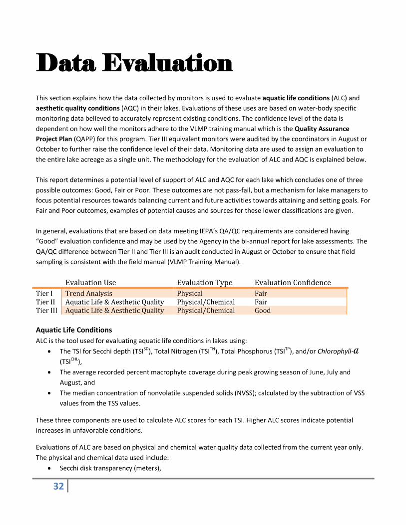
32
Data Evaluation
This section explains how the data collected by monitors is used to evaluate aquatic life conditions (ALC) and
aesthetic quality conditions (AQC) in their lakes. Evaluations of these uses are based on water-body specific
monitoring data believed to accurately represent existing conditions. The confidence level of the data is
dependent on how well the monitors adhere to the VLMP training manual which is the Quality Assurance
Project Plan (QAPP) for this program. Tier III equivalent monitors were audited by the coordinators in August or
October to further raise the confidence level of their data. Monitoring data are used to assign an evaluation to
the entire lake acreage as a single unit. The methodology for the evaluation of ALC and AQC is explained below.
This report determines a potential level of support of ALC and AQC for each lake which concludes one of three
possible outcomes: Good, Fair or Poor. These outcomes are not pass-fail, but a mechanism for lake managers to
focus potential resources towards balancing current and future activities towards attaining and setting goals. For
Fair and Poor outcomes, examples of potential causes and sources for these lower classifications are given.
In general, evaluations that are based on data meeting IEPA’s QA/QC requirements are considered having
“Good” evaluation confidence and may be used by the Agency in the bi-annual report for lake assessments. The
QA/QC difference between Tier II and Tier III is an audit conducted in August or October to ensure that field
sampling is consistent with the field manual (VLMP Training Manual).
Evaluation Use Evaluation Type Evaluation Confidence
Tier I Trend Analysis Physical Fair Tier II Aquatic Life & Aesthetic Quality Physical/Chemical Fair Tier III Aquatic Life & Aesthetic Quality Physical/Chemical Good
Aquatic Life Conditions
ALC is the tool used for evaluating aquatic life conditions in lakes using:
The TSI for Secchi depth (TSISD), Total Nitrogen (TSITN), Total Phosphorus (TSITP), and/or Chlorophyll-A
(TSICHL),
The average recorded percent macrophyte coverage during peak growing season of June, July and
August, and
The median concentration of nonvolatile suspended solids (NVSS); calculated by the subtraction of VSS
values from the TSS values.
These three components are used to calculate ALC scores for each TSI. Higher ALC scores indicate potential
increases in unfavorable conditions.
Evaluations of ALC are based on physical and chemical water quality data collected from the current year only.
The physical and chemical data used include:
Secchi disk transparency (meters),
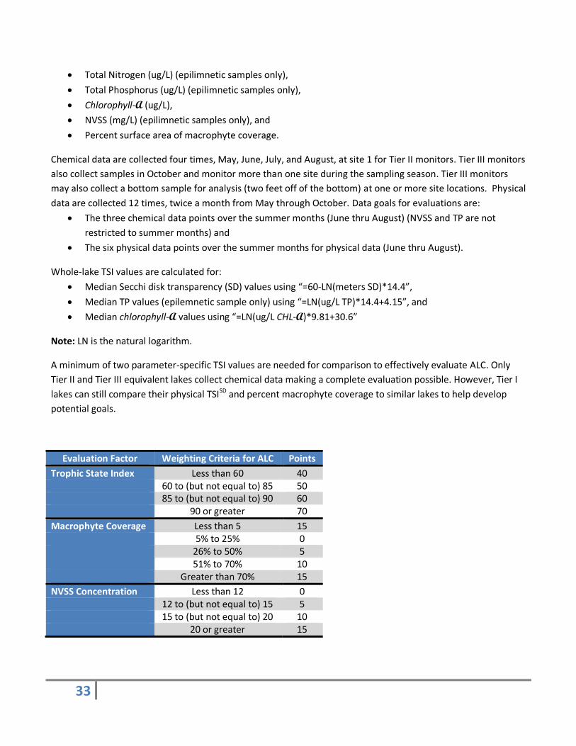
33
Total Nitrogen (ug/L) (epilimnetic samples only),
Total Phosphorus (ug/L) (epilimnetic samples only),
Chlorophyll-A (ug/L),
NVSS (mg/L) (epilimnetic samples only), and
Percent surface area of macrophyte coverage.
Chemical data are collected four times, May, June, July, and August, at site 1 for Tier II monitors. Tier III monitors
also collect samples in October and monitor more than one site during the sampling season. Tier III monitors
may also collect a bottom sample for analysis (two feet off of the bottom) at one or more site locations. Physical
data are collected 12 times, twice a month from May through October. Data goals for evaluations are:
The three chemical data points over the summer months (June thru August) (NVSS and TP are not
restricted to summer months) and
The six physical data points over the summer months for physical data (June thru August).
Whole-lake TSI values are calculated for:
Median Secchi disk transparency (SD) values using “=60-LN(meters SD)*14.4”,
Median TP values (epilemnetic sample only) using “=LN(ug/L TP)*14.4+4.15”, and
Median chlorophyll-A values using “=LN(ug/L CHL-A)*9.81+30.6”
Note: LN is the natural logarithm.
A minimum of two parameter-specific TSI values are needed for comparison to effectively evaluate ALC. Only
Tier II and Tier III equivalent lakes collect chemical data making a complete evaluation possible. However, Tier I
lakes can still compare their physical TSISD and percent macrophyte coverage to similar lakes to help develop
potential goals.
Evaluation Factor Weighting Criteria for ALC Points
Trophic State Index Less than 60 40 60 to (but not equal to) 85 50 85 to (but not equal to) 90 60 90 or greater 70
Macrophyte Coverage Less than 5 15 5% to 25% 0 26% to 50% 5 51% to 70% 10 Greater than 70% 15
NVSS Concentration Less than 12 0 12 to (but not equal to) 15 5 15 to (but not equal to) 20 10 20 or greater 15
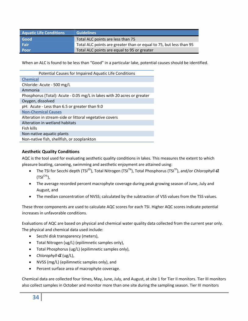
34
Aquatic Life Conditions Guidelines
Good Total ALC points are less than 75 Fair Total ALC points are greater than or equal to 75, but less than 95 Poor Total ALC points are equal to 95 or greater
When an ALC is found to be less than “Good” in a particular lake, potential causes should be identified.
Potential Causes for Impaired Aquatic Life Conditions
Chemical Chloride: Acute - 500 mg/L Ammonia Phosphorus (Total): Acute - 0.05 mg/L in lakes with 20 acres or greater Oxygen, dissolved pH: Acute - Less than 6.5 or greater than 9.0 Non-Chemical Causes Alteration in stream-side or littoral vegetative covers Alteration in wetland habitats Fish kills Non-native aquatic plants Non-native fish, shellfish, or zooplankton
Aesthetic Quality Conditions
AQC is the tool used for evaluating aesthetic quality conditions in lakes. This measures the extent to which
pleasure boating, canoeing, swimming and aesthetic enjoyment are attained using:
The TSI for Secchi depth (TSISD), Total Nitrogen (TSITN), Total Phosphorus (TSITP), and/or Chlorophyll-A
(TSICHL),
The average recorded percent macrophyte coverage during peak growing season of June, July and
August, and
The median concentration of NVSS; calculated by the subtraction of VSS values from the TSS values.
These three components are used to calculate AQC scores for each TSI. Higher AQC scores indicate potential
increases in unfavorable conditions.
Evaluations of AQC are based on physical and chemical water quality data collected from the current year only.
The physical and chemical data used include:
Secchi disk transparency (meters),
Total Nitrogen (ug/L) (epilimnetic samples only),
Total Phosphorus (ug/L) (epilimnetic samples only),
Chlorophyll-A (ug/L),
NVSS (mg/L) (epilimnetic samples only), and
Percent surface area of macrophyte coverage.
Chemical data are collected four times, May, June, July, and August, at site 1 for Tier II monitors. Tier III monitors
also collect samples in October and monitor more than one site during the sampling season. Tier III monitors
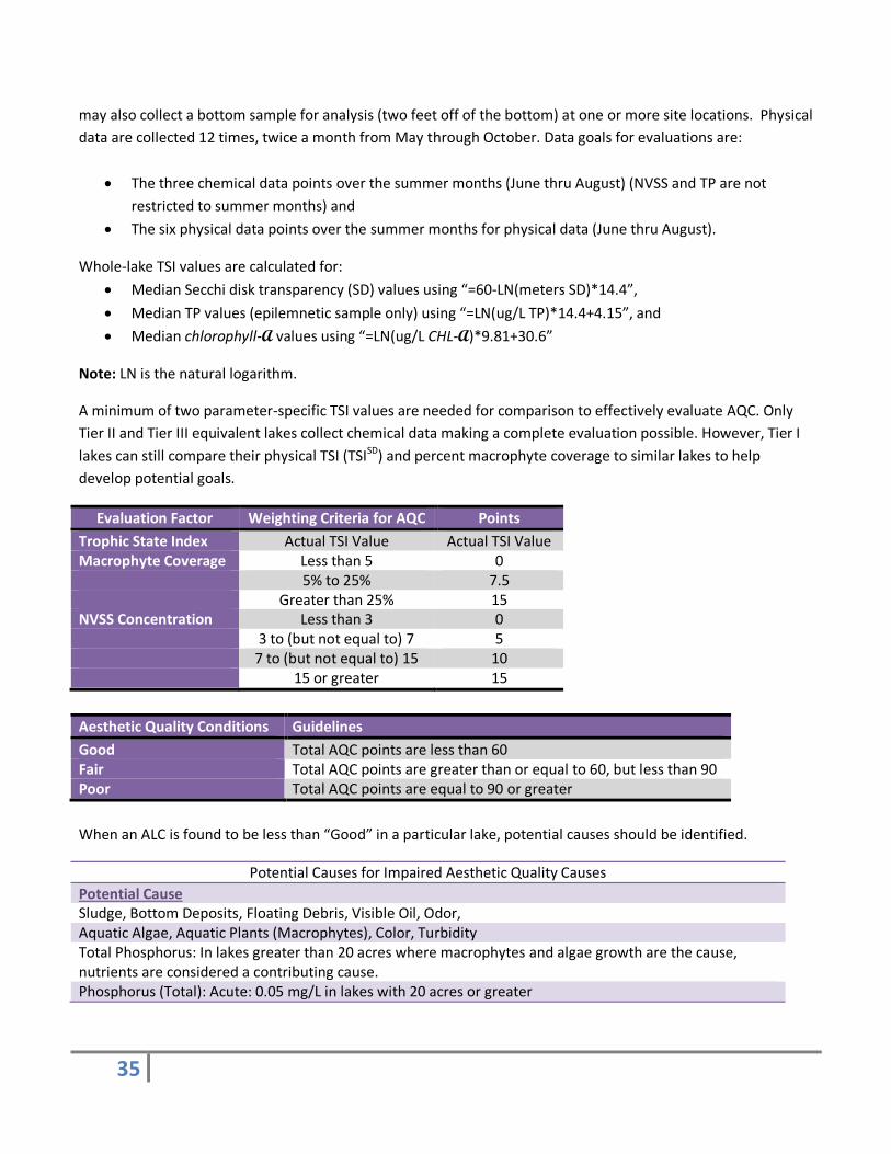
35
may also collect a bottom sample for analysis (two feet off of the bottom) at one or more site locations. Physical
data are collected 12 times, twice a month from May through October. Data goals for evaluations are:
The three chemical data points over the summer months (June thru August) (NVSS and TP are not
restricted to summer months) and
The six physical data points over the summer months for physical data (June thru August).
Whole-lake TSI values are calculated for:
Median Secchi disk transparency (SD) values using “=60-LN(meters SD)*14.4”,
Median TP values (epilemnetic sample only) using “=LN(ug/L TP)*14.4+4.15”, and
Median chlorophyll-A values using “=LN(ug/L CHL-A)*9.81+30.6”
Note: LN is the natural logarithm.
A minimum of two parameter-specific TSI values are needed for comparison to effectively evaluate AQC. Only
Tier II and Tier III equivalent lakes collect chemical data making a complete evaluation possible. However, Tier I
lakes can still compare their physical TSI (TSISD) and percent macrophyte coverage to similar lakes to help
develop potential goals.
Evaluation Factor Weighting Criteria for AQC Points
Trophic State Index Actual TSI Value Actual TSI Value Macrophyte Coverage Less than 5 0 5% to 25% 7.5 Greater than 25% 15 NVSS Concentration Less than 3 0 3 to (but not equal to) 7 5 7 to (but not equal to) 15 10 15 or greater 15
Aesthetic Quality Conditions Guidelines
Good Total AQC points are less than 60 Fair Total AQC points are greater than or equal to 60, but less than 90 Poor Total AQC points are equal to 90 or greater
When an ALC is found to be less than “Good” in a particular lake, potential causes should be identified.
Potential Causes for Impaired Aesthetic Quality Causes
Potential Cause Sludge, Bottom Deposits, Floating Debris, Visible Oil, Odor, Aquatic Algae, Aquatic Plants (Macrophytes), Color, Turbidity Total Phosphorus: In lakes greater than 20 acres where macrophytes and algae growth are the cause, nutrients are considered a contributing cause. Phosphorus (Total): Acute: 0.05 mg/L in lakes with 20 acres or greater
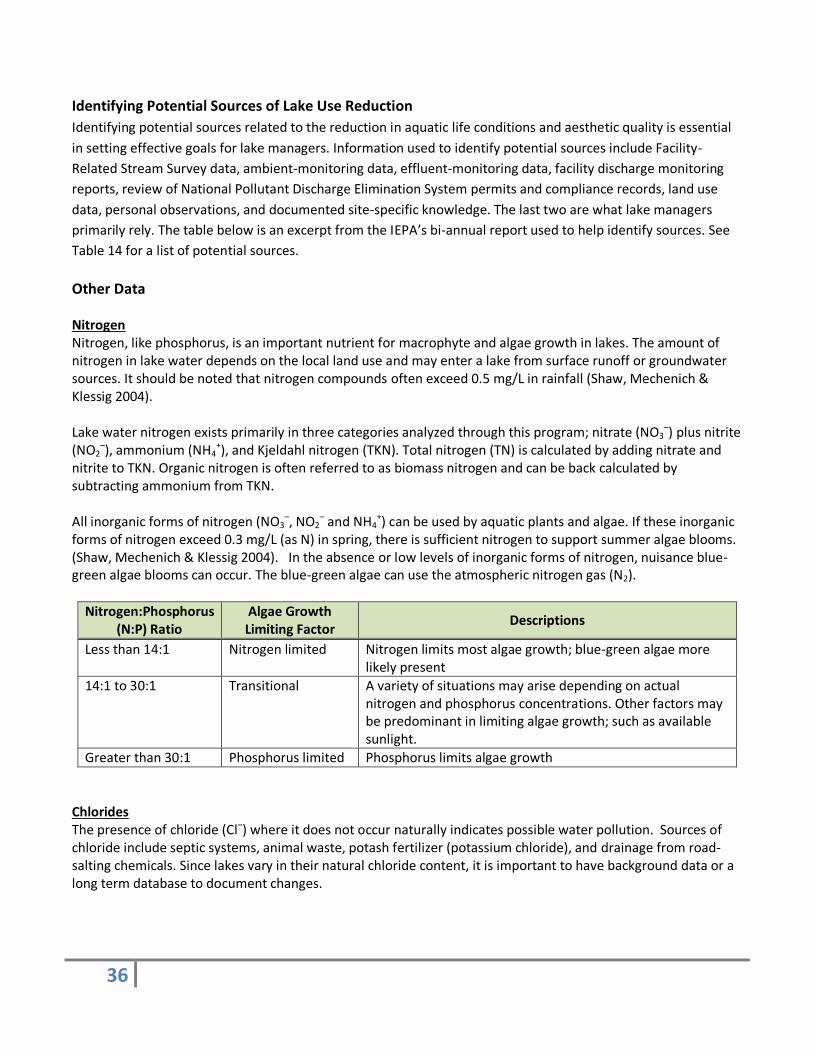
36
Identifying Potential Sources of Lake Use Reduction
Identifying potential sources related to the reduction in aquatic life conditions and aesthetic quality is essential
in setting effective goals for lake managers. Information used to identify potential sources include Facility-
Related Stream Survey data, ambient-monitoring data, effluent-monitoring data, facility discharge monitoring
reports, review of National Pollutant Discharge Elimination System permits and compliance records, land use
data, personal observations, and documented site-specific knowledge. The last two are what lake managers
primarily rely. The table below is an excerpt from the IEPA’s bi-annual report used to help identify sources. See
Table 14 for a list of potential sources.
Other Data Nitrogen Nitrogen, like phosphorus, is an important nutrient for macrophyte and algae growth in lakes. The amount of nitrogen in lake water depends on the local land use and may enter a lake from surface runoff or groundwater sources. It should be noted that nitrogen compounds often exceed 0.5 mg/L in rainfall (Shaw, Mechenich & Klessig 2004). Lake water nitrogen exists primarily in three categories analyzed through this program; nitrate (NO3
–) plus nitrite (NO2
–), ammonium (NH4+), and Kjeldahl nitrogen (TKN). Total nitrogen (TN) is calculated by adding nitrate and
nitrite to TKN. Organic nitrogen is often referred to as biomass nitrogen and can be back calculated by subtracting ammonium from TKN. All inorganic forms of nitrogen (NO3
–, NO2– and NH4
+) can be used by aquatic plants and algae. If these inorganic forms of nitrogen exceed 0.3 mg/L (as N) in spring, there is sufficient nitrogen to support summer algae blooms. (Shaw, Mechenich & Klessig 2004). In the absence or low levels of inorganic forms of nitrogen, nuisance blue-green algae blooms can occur. The blue-green algae can use the atmospheric nitrogen gas (N2).
Nitrogen:Phosphorus (N:P) Ratio
Algae Growth Limiting Factor
Descriptions
Less than 14:1 Nitrogen limited Nitrogen limits most algae growth; blue-green algae more likely present
14:1 to 30:1 Transitional A variety of situations may arise depending on actual nitrogen and phosphorus concentrations. Other factors may be predominant in limiting algae growth; such as available sunlight.
Greater than 30:1 Phosphorus limited Phosphorus limits algae growth
Chlorides The presence of chloride (Cl–) where it does not occur naturally indicates possible water pollution. Sources of chloride include septic systems, animal waste, potash fertilizer (potassium chloride), and drainage from road-salting chemicals. Since lakes vary in their natural chloride content, it is important to have background data or a long term database to document changes.
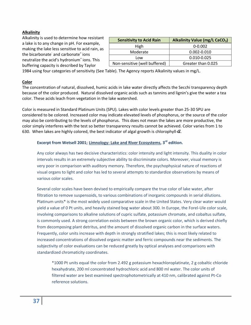
37
Alkalinity Alkalinity is used to determine how resistant a lake is to any change in pH. For example, making the lake less sensitive to acid rain, as the bicarbonate- and carbonate= ions neutralize the acid’s hydronium+ ions. This buffering capacity is described by Taylor 1984 using four categories of sensitivity (See Table). The Agency reports Alkalinity values in mg/L. Color The concentration of natural, dissolved, humic acids in lake water directly affects the Secchi transparency depth because of the color produced. Natural dissolved organic acids such as tannins and lignin’s give the water a tea color. These acids leach from vegetation in the lake watershed. Color is measured in Standard Platinum Units (SPU). Lakes with color levels greater than 25-30 SPU are considered to be colored. Increased color may indicate elevated levels of phosphorus, or the source of the color may also be contributing to the levels of phosphorus. This does not mean the lakes are more productive, the color simply interferes with the test so better transparency results cannot be achieved. Color varies from 1 to 630. When lakes are highly colored, the best indicator of algal growth is chlorophyll-A.
Excerpt from Wetsell 2001; Limnology: Lake and River Ecosystems, 3rd edition.
Any color always has two decisive characteristics: color intensity and light intensity. This duality in color
intervals results in an extremely subjective ability to discriminate colors. Moreover, visual memory is
very poor in comparison with auditory memory. Therefore, the psychophysical nature of reactions of
visual organs to light and color has led to several attempts to standardize observations by means of
various color scales.
Several color scales have been devised to empirically compare the true color of lake water, after
filtration to remove suspensoids, to various combinations of inorganic compounds in serial dilutions.
Platinum units* is the most widely used comparative scale in the United States. Very clear water would
yield a value of 0 Pt units, and heavily stained bog water about 300. In Europe, the Forel-Ule color scale,
involving comparisons to alkaline solutions of cupric sulfate, potassium chromate, and cobaltus sulfate,
is commonly used. A strong correlation exists between the brown organic color, which is derived chiefly
from decomposing plant detritus, and the amount of dissolved organic carbon in the surface waters.
Frequently, color units increase with depth in strongly stratified lakes; this is most likely related to
increased concentrations of dissolved organic matter and ferric compounds near the sediments. The
subjectivity of color evaluations can be reduced greatly by optical analyses and comparisons with
standardized chromaticity coordinates.
*1000 Pt units equal the color from 2.492 g potassium hexachloroplatinate, 2 g cobaltic chloride
hexahydrate, 200 ml concentrated hydrochloric acid and 800 ml water. The color units of
filtered water are best examined spectrophotometrically at 410 nm, calibrated against Pt-Co
reference solutions.
Sensitivity to Acid Rain Alkalinity Value (mg/L CaCO3)
High 0-0.002
Moderate 0.002-0.010
Low 0.010-0.025
Non-sensitive (well buffered) Greater than 0.025
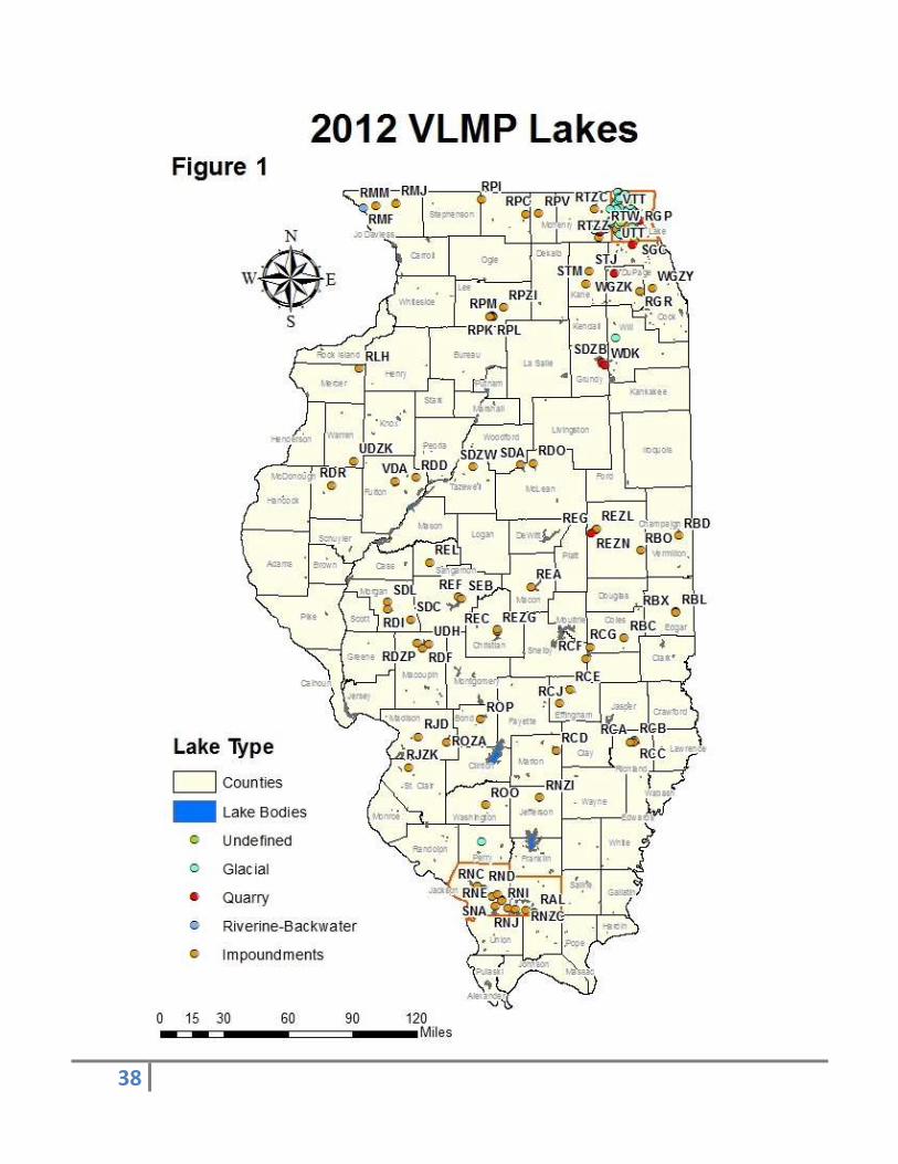
38
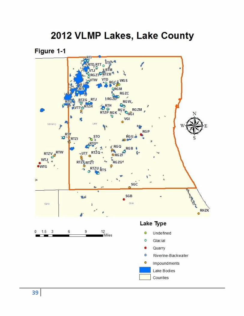
39
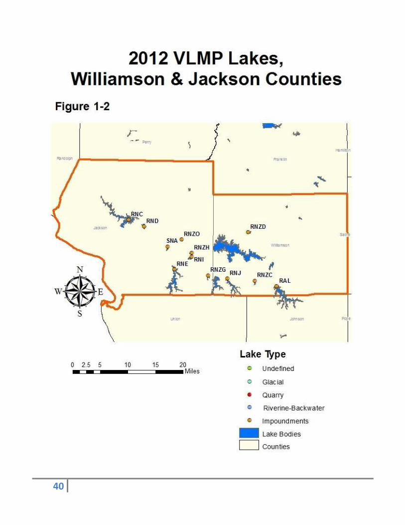
40
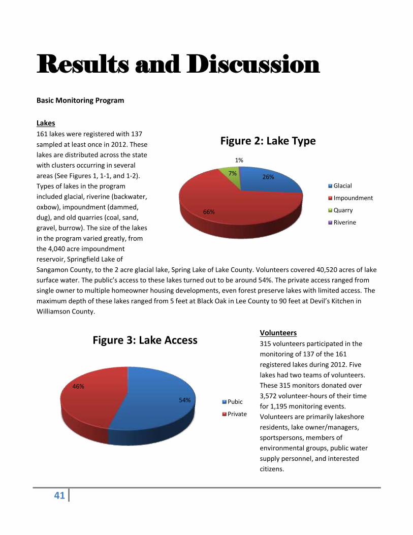
41
Results and Discussion
Basic Monitoring Program
Lakes
161 lakes were registered with 137
sampled at least once in 2012. These
lakes are distributed across the state
with clusters occurring in several
areas (See Figures 1, 1-1, and 1-2).
Types of lakes in the program
included glacial, riverine (backwater,
oxbow), impoundment (dammed,
dug), and old quarries (coal, sand,
gravel, burrow). The size of the lakes
in the program varied greatly, from
the 4,040 acre impoundment
reservoir, Springfield Lake of
Sangamon County, to the 2 acre glacial lake, Spring Lake of Lake County. Volunteers covered 40,520 acres of lake
surface water. The public’s access to these lakes turned out to be around 54%. The private access ranged from
single owner to multiple homeowner housing developments, even forest preserve lakes with limited access. The
maximum depth of these lakes ranged from 5 feet at Black Oak in Lee County to 90 feet at Devil’s Kitchen in
Williamson County.
Volunteers
315 volunteers participated in the
monitoring of 137 of the 161
registered lakes during 2012. Five
lakes had two teams of volunteers.
These 315 monitors donated over
3,572 volunteer-hours of their time
for 1,195 monitoring events.
Volunteers are primarily lakeshore
residents, lake owner/managers,
sportspersons, members of
environmental groups, public water
supply personnel, and interested
citizens.
26%
66%
7%
1%
Figure 2: Lake Type
Glacial
Impoundment
Quarry
Riverine
54%
46%
Figure 3: Lake Access
Pubic
Private
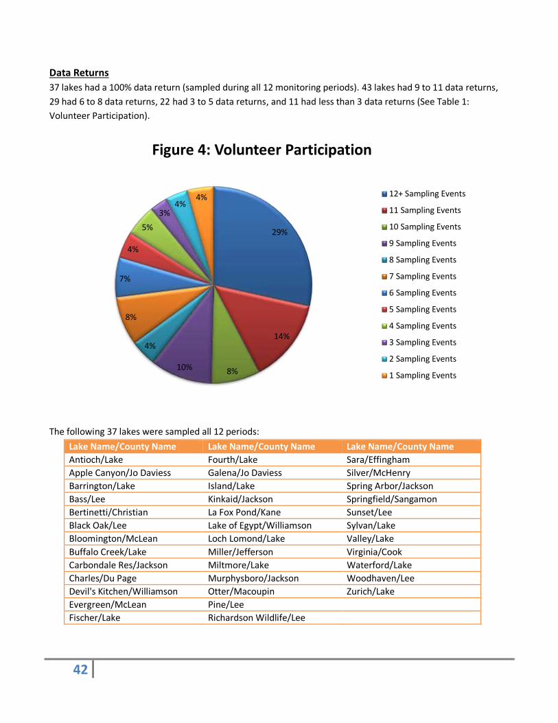
42
Data Returns
37 lakes had a 100% data return (sampled during all 12 monitoring periods). 43 lakes had 9 to 11 data returns,
29 had 6 to 8 data returns, 22 had 3 to 5 data returns, and 11 had less than 3 data returns (See Table 1:
Volunteer Participation).
The following 37 lakes were sampled all 12 periods:
Lake Name/County Name Lake Name/County Name Lake Name/County Name
Antioch/Lake Fourth/Lake Sara/Effingham
Apple Canyon/Jo Daviess Galena/Jo Daviess Silver/McHenry
Barrington/Lake Island/Lake Spring Arbor/Jackson
Bass/Lee Kinkaid/Jackson Springfield/Sangamon
Bertinetti/Christian La Fox Pond/Kane Sunset/Lee
Black Oak/Lee Lake of Egypt/Williamson Sylvan/Lake
Bloomington/McLean Loch Lomond/Lake Valley/Lake
Buffalo Creek/Lake Miller/Jefferson Virginia/Cook
Carbondale Res/Jackson Miltmore/Lake Waterford/Lake
Charles/Du Page Murphysboro/Jackson Woodhaven/Lee
Devil's Kitchen/Williamson Otter/Macoupin Zurich/Lake
Evergreen/McLean Pine/Lee
Fischer/Lake Richardson Wildlife/Lee
29%
14%
8% 10%
4%
8%
7%
4%
5%
3% 4%
4%
Figure 4: Volunteer Participation
12+ Sampling Events
11 Sampling Events
10 Sampling Events
9 Sampling Events
8 Sampling Events
7 Sampling Events
6 Sampling Events
5 Sampling Events
4 Sampling Events
3 Sampling Events
2 Sampling Events
1 Sampling Events
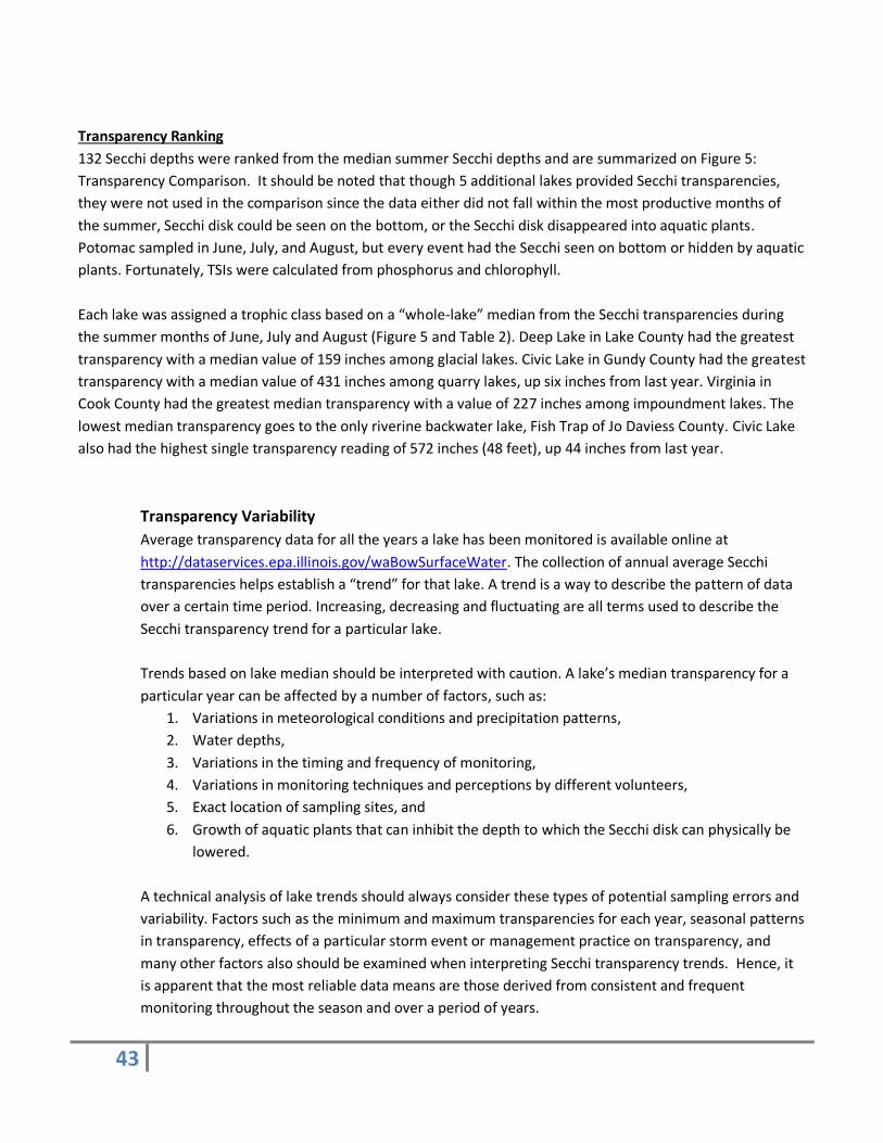
43
Transparency Ranking
132 Secchi depths were ranked from the median summer Secchi depths and are summarized on Figure 5:
Transparency Comparison. It should be noted that though 5 additional lakes provided Secchi transparencies,
they were not used in the comparison since the data either did not fall within the most productive months of
the summer, Secchi disk could be seen on the bottom, or the Secchi disk disappeared into aquatic plants.
Potomac sampled in June, July, and August, but every event had the Secchi seen on bottom or hidden by aquatic
plants. Fortunately, TSIs were calculated from phosphorus and chlorophyll.
Each lake was assigned a trophic class based on a “whole-lake” median from the Secchi transparencies during
the summer months of June, July and August (Figure 5 and Table 2). Deep Lake in Lake County had the greatest
transparency with a median value of 159 inches among glacial lakes. Civic Lake in Gundy County had the greatest
transparency with a median value of 431 inches among quarry lakes, up six inches from last year. Virginia in
Cook County had the greatest median transparency with a value of 227 inches among impoundment lakes. The
lowest median transparency goes to the only riverine backwater lake, Fish Trap of Jo Daviess County. Civic Lake
also had the highest single transparency reading of 572 inches (48 feet), up 44 inches from last year.
Transparency Variability
Average transparency data for all the years a lake has been monitored is available online at
http://dataservices.epa.illinois.gov/waBowSurfaceWater. The collection of annual average Secchi
transparencies helps establish a “trend” for that lake. A trend is a way to describe the pattern of data
over a certain time period. Increasing, decreasing and fluctuating are all terms used to describe the
Secchi transparency trend for a particular lake.
Trends based on lake median should be interpreted with caution. A lake’s median transparency for a
particular year can be affected by a number of factors, such as:
1. Variations in meteorological conditions and precipitation patterns,
2. Water depths,
3. Variations in the timing and frequency of monitoring,
4. Variations in monitoring techniques and perceptions by different volunteers,
5. Exact location of sampling sites, and
6. Growth of aquatic plants that can inhibit the depth to which the Secchi disk can physically be
lowered.
A technical analysis of lake trends should always consider these types of potential sampling errors and
variability. Factors such as the minimum and maximum transparencies for each year, seasonal patterns
in transparency, effects of a particular storm event or management practice on transparency, and
many other factors also should be examined when interpreting Secchi transparency trends. Hence, it
is apparent that the most reliable data means are those derived from consistent and frequent
monitoring throughout the season and over a period of years.
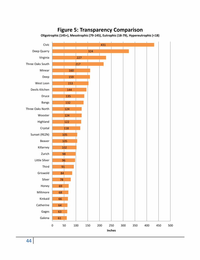
44
61
63
64
66
68
69
78
84
91
96
98
102
105
105
118
122
124
124
132
135
144
153
159
160
217
227
324
431
0 50 100 150 200 250 300 350 400 450 500
Galena
Gages
Catherine
Kinkaid
Miltmore
Honey
Silver
Griswold
Third
Little Silver
Zurich
Killarney
Beaver
Sunset (REZN)
Crystal
Highland
Wooster
Three Oaks North
Bangs
Druce
Devils Kitchen
West Loon
Deep
Minear
Three Oaks South
Virginia
Deep Quarry
Civic
Inches
Figure 5: Transparency Comparison Oligotrophic (145+), Mesotrophic (79-145), Eutrophic (18-79), Hypereutrophic (<18)
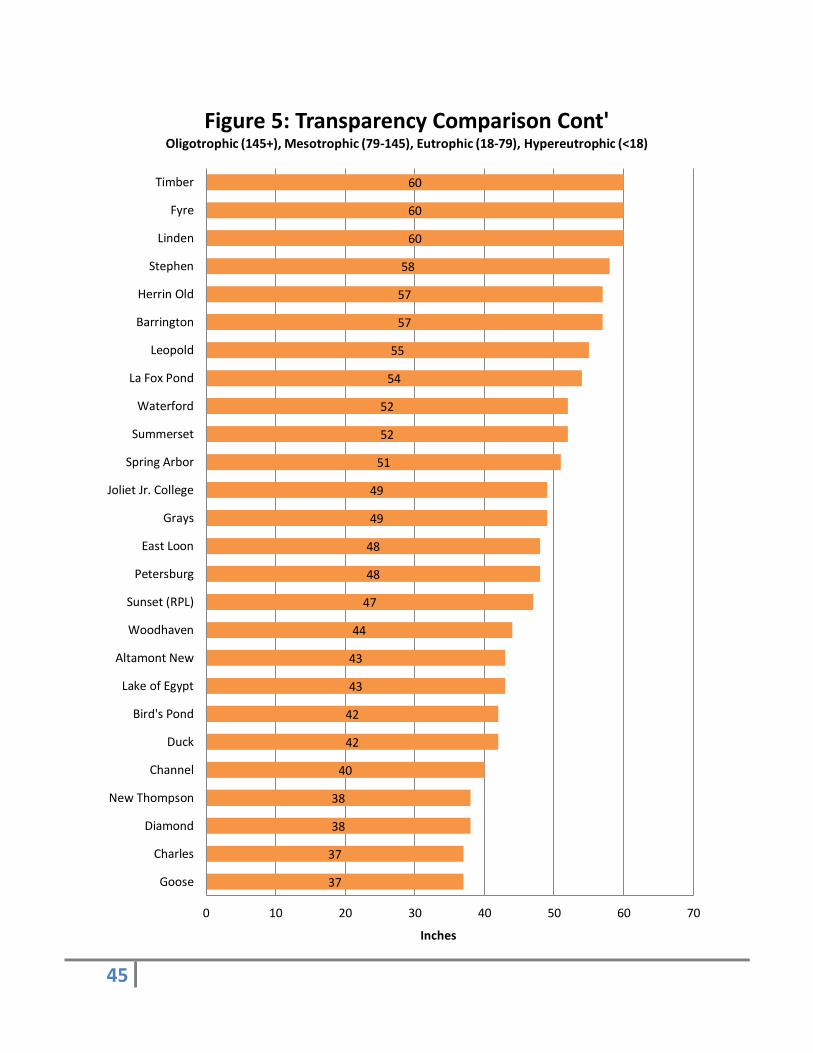
45
37
37
38
38
40
42
42
43
43
44
47
48
48
49
49
51
52
52
54
55
57
57
58
60
60
60
0 10 20 30 40 50 60 70
Goose
Charles
Diamond
New Thompson
Channel
Duck
Bird's Pond
Lake of Egypt
Altamont New
Woodhaven
Sunset (RPL)
Petersburg
East Loon
Grays
Joliet Jr. College
Spring Arbor
Summerset
Waterford
La Fox Pond
Leopold
Barrington
Herrin Old
Stephen
Linden
Fyre
Timber
Inches
Figure 5: Transparency Comparison Cont' Oligotrophic (145+), Mesotrophic (79-145), Eutrophic (18-79), Hypereutrophic (<18)
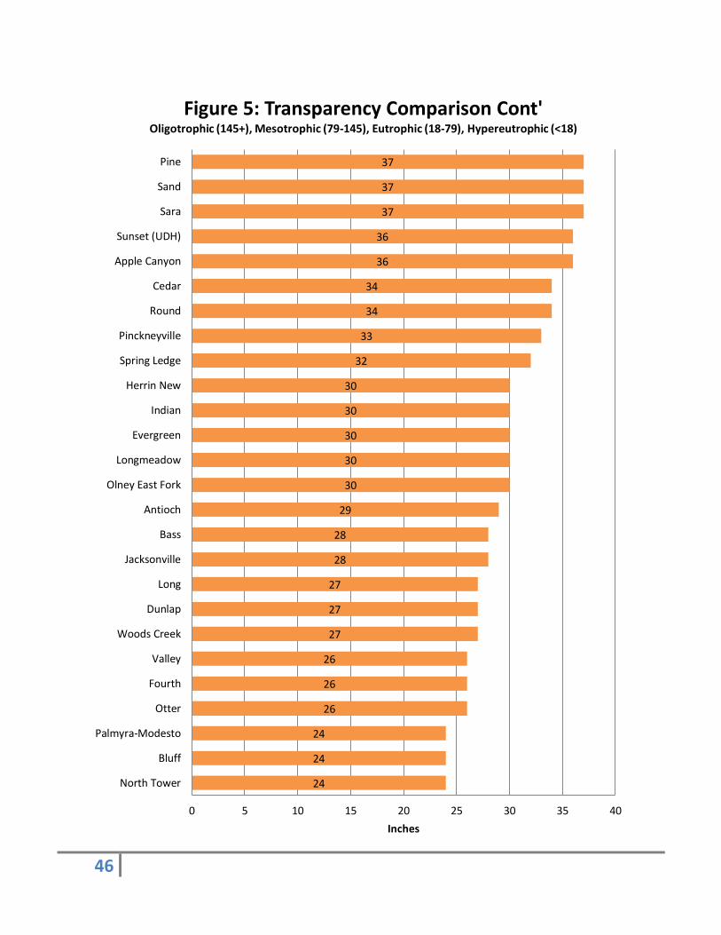
46
24
24
24
26
26
26
27
27
27
28
28
29
30
30
30
30
30
32
33
34
34
36
36
37
37
37
0 5 10 15 20 25 30 35 40
North Tower
Bluff
Palmyra-Modesto
Otter
Fourth
Valley
Woods Creek
Dunlap
Long
Jacksonville
Bass
Antioch
Olney East Fork
Longmeadow
Evergreen
Indian
Herrin New
Spring Ledge
Pinckneyville
Round
Cedar
Apple Canyon
Sunset (UDH)
Sara
Sand
Pine
Inches
Figure 5: Transparency Comparison Cont' Oligotrophic (145+), Mesotrophic (79-145), Eutrophic (18-79), Hypereutrophic (<18)
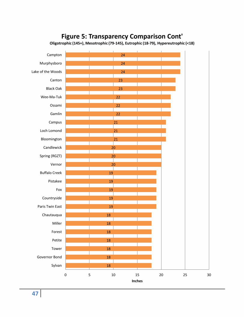
47
18
18
18
18
18
18
18
19
19
19
19
19
20
20
20
21
21
21
22
22
22
23
23
24
24
24
0 5 10 15 20 25 30
Sylvan
Governor Bond
Tower
Petite
Forest
Miller
Chautauqua
Paris Twin East
Countryside
Fox
Pistakee
Buffalo Creek
Vernor
Spring (RGZT)
Candlewick
Bloomington
Loch Lomond
Campus
Gamlin
Ossami
Wee-Ma-Tuk
Black Oak
Canton
Lake of the Woods
Murphysboro
Campton
Inches
Figure 5: Transparency Comparison Cont' Oligotrophic (145+), Mesotrophic (79-145), Eutrophic (18-79), Hypereutrophic (<18)
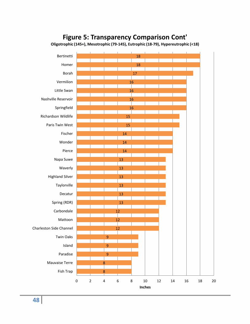
48
8
8
9
9
9
12
12
12
13
13
13
13
13
13
14
14
14
15
15
16
16
16
16
17
18
18
0 2 4 6 8 10 12 14 16 18 20
Fish Trap
Mauvaise Terre
Paradise
Island
Twin Oaks
Charleston Side Channel
Mattoon
Carbondale
Spring (RDR)
Decatur
Taylorville
Highland Silver
Waverly
Napa Suwe
Pierce
Wonder
Fischer
Paris Twin West
Richardson Wildlife
Springfield
Nashville Reservoir
Little Swan
Vermilion
Borah
Homer
Bertinetti
Inches
Figure 5: Transparency Comparison Cont' Oligotrophic (145+), Mesotrophic (79-145), Eutrophic (18-79), Hypereutrophic (<18)
49
% Macrophyte Results
Volunteers make an estimate of the % coverage of macrophytes (aquatic plants) on a lake. Each range is given a
weighted point value in regards to whether that coverage range is good (0 points) to poor (15 points) for
“Aquatic Life conditions” and “Aesthetic Quality conditions.” See Table 3: Macrophyte Coverage Totals.
Aquatic Life conditions Weighting Criteria
Points Aesthetic Quality conditions Weighting Criteria
Points
Less than 5% 15 Less Than 5% 0 5% to 25% 0 5% to 25% 7.5
26% to 50% 5 26% to 50% 15 51% to 70% 10 51% to 70% 15
Greater Than 70% 15 Greater Than 70% 15
Expanded Monitoring Programs
Water Quality Monitoring
In 2012, volunteers at 83 lakes collected water samples from one foot below the lake water surface. Water
quality data are summarized in tables, see Appendix D. Not all samples were analyzed for all constituents.
Chloride analysis was limited to the general Chicago metropolitan area of Cook, Du Page, Kane, Kendall, Lake,
McHenry, and Will counties. Some samples
Chlorophyll-A: 73 lake TSICHL‘s were calculated from the chlorophyll data and are summarized in Table 4:
Trophic State Indexes.
Total Phosphorus: 53 of the 82 lakes had median values of TP over the 0.05 mg/L. It should be noted that
eight of the lakes with medians under the 0.05 mg/L TP had one or more sampling events with TP levels
over that benchmark. 82 lake TSITP‘s were calculated and are summarized in Table 4: Trophic State Indexes.
Alkalinity: All 78 lakes analyzed for alkalinity appear to be well buffered, with a range of 25 mg/L at Devil’s
Kitchen in Williamson County to 365 mg/L at Wooster in Lake County.
Non-volatile Suspended Solids: 81 lake NVSS median values were calculated from TSS & VSS. Table 5
summarizes these median values and assigns weighted points for evaluating its effects on aquatic life and
aesthetic quality. 50 lakes showed no significant amounts of NVSS, less than 3 mg/L.
Color: 81 lakes were analyzed for true color. Values ranged from a justified value of 0.09 C.U.s to 79 C.U.s.
The median range ran from a justified value (value below the method’s detection limit) of 2 C.U. for Deep
Quarry/Du Page, Three Oaks South/McHenry, Civic/Grundy and Sunset/Champaign to 36 C.U. for Island
Lake in McHenry and Lake Counties. It is interesting to note that the four lakes with 2 C.U.s are all quarry
lakes.
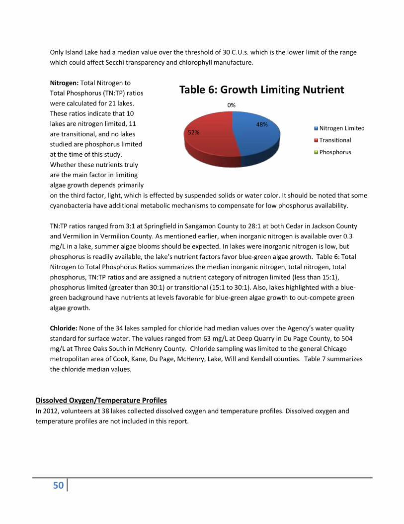
50
Only Island Lake had a median value over the threshold of 30 C.U.s. which is the lower limit of the range
which could affect Secchi transparency and chlorophyll manufacture.
Nitrogen: Total Nitrogen to
Total Phosphorus (TN:TP) ratios
were calculated for 21 lakes.
These ratios indicate that 10
lakes are nitrogen limited, 11
are transitional, and no lakes
studied are phosphorus limited
at the time of this study.
Whether these nutrients truly
are the main factor in limiting
algae growth depends primarily
on the third factor, light, which is effected by suspended solids or water color. It should be noted that some
cyanobacteria have additional metabolic mechanisms to compensate for low phosphorus availability.
TN:TP ratios ranged from 3:1 at Springfield in Sangamon County to 28:1 at both Cedar in Jackson County
and Vermilion in Vermilion County. As mentioned earlier, when inorganic nitrogen is available over 0.3
mg/L in a lake, summer algae blooms should be expected. In lakes were inorganic nitrogen is low, but
phosphorus is readily available, the lake’s nutrient factors favor blue-green algae growth. Table 6: Total
Nitrogen to Total Phosphorus Ratios summarizes the median inorganic nitrogen, total nitrogen, total
phosphorus, TN:TP ratios and are assigned a nutrient category of nitrogen limited (less than 15:1),
phosphorus limited (greater than 30:1) or transitional (15:1 to 30:1). Also, lakes highlighted with a blue-
green background have nutrients at levels favorable for blue-green algae growth to out-compete green
algae growth.
Chloride: None of the 34 lakes sampled for chloride had median values over the Agency’s water quality
standard for surface water. The values ranged from 63 mg/L at Deep Quarry in Du Page County, to 504
mg/L at Three Oaks South in McHenry County. Chloride sampling was limited to the general Chicago
metropolitan area of Cook, Kane, Du Page, McHenry, Lake, Will and Kendall counties. Table 7 summarizes
the chloride median values.
Dissolved Oxygen/Temperature Profiles
In 2012, volunteers at 38 lakes collected dissolved oxygen and temperature profiles. Dissolved oxygen and
temperature profiles are not included in this report.
48% 52%
0%
Table 6: Growth Limiting Nutrient
Nitrogen Limited
Transitional
Phosphorus
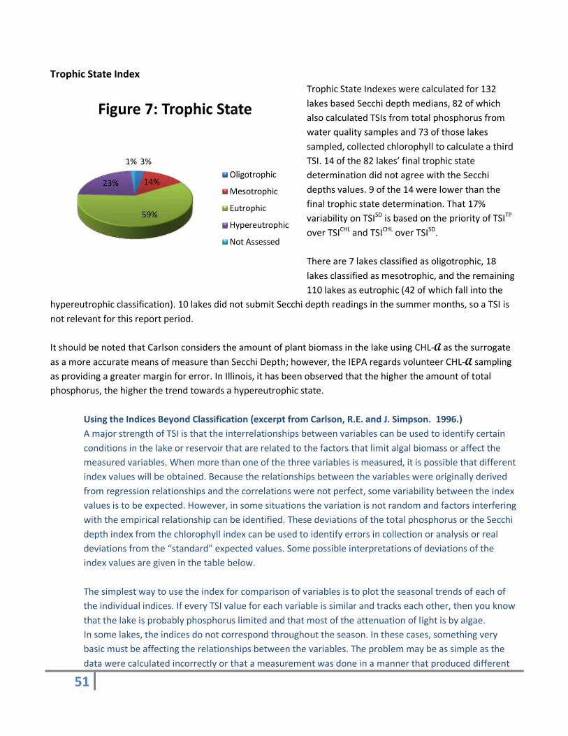
51
Trophic State Index
Trophic State Indexes were calculated for 132
lakes based Secchi depth medians, 82 of which
also calculated TSIs from total phosphorus from
water quality samples and 73 of those lakes
sampled, collected chlorophyll to calculate a third
TSI. 14 of the 82 lakes’ final trophic state
determination did not agree with the Secchi
depths values. 9 of the 14 were lower than the
final trophic state determination. That 17%
variability on TSISD is based on the priority of TSITP
over TSICHL and TSICHL over TSISD.
There are 7 lakes classified as oligotrophic, 18
lakes classified as mesotrophic, and the remaining
110 lakes as eutrophic (42 of which fall into the
hypereutrophic classification). 10 lakes did not submit Secchi depth readings in the summer months, so a TSI is
not relevant for this report period.
It should be noted that Carlson considers the amount of plant biomass in the lake using CHL-A as the surrogate
as a more accurate means of measure than Secchi Depth; however, the IEPA regards volunteer CHL-A sampling
as providing a greater margin for error. In Illinois, it has been observed that the higher the amount of total
phosphorus, the higher the trend towards a hypereutrophic state.
Using the Indices Beyond Classification (excerpt from Carlson, R.E. and J. Simpson. 1996.)
A major strength of TSI is that the interrelationships between variables can be used to identify certain
conditions in the lake or reservoir that are related to the factors that limit algal biomass or affect the
measured variables. When more than one of the three variables is measured, it is possible that different
index values will be obtained. Because the relationships between the variables were originally derived
from regression relationships and the correlations were not perfect, some variability between the index
values is to be expected. However, in some situations the variation is not random and factors interfering
with the empirical relationship can be identified. These deviations of the total phosphorus or the Secchi
depth index from the chlorophyll index can be used to identify errors in collection or analysis or real
deviations from the “standard” expected values. Some possible interpretations of deviations of the
index values are given in the table below.
The simplest way to use the index for comparison of variables is to plot the seasonal trends of each of
the individual indices. If every TSI value for each variable is similar and tracks each other, then you know
that the lake is probably phosphorus limited and that most of the attenuation of light is by algae.
In some lakes, the indices do not correspond throughout the season. In these cases, something very
basic must be affecting the relationships between the variables. The problem may be as simple as the
data were calculated incorrectly or that a measurement was done in a manner that produced different
3%
14%
59%
23%
1%
Figure 7: Trophic State
Oligotrophic
Mesotrophic
Eutrophic
Hypereutrophic
Not Assessed
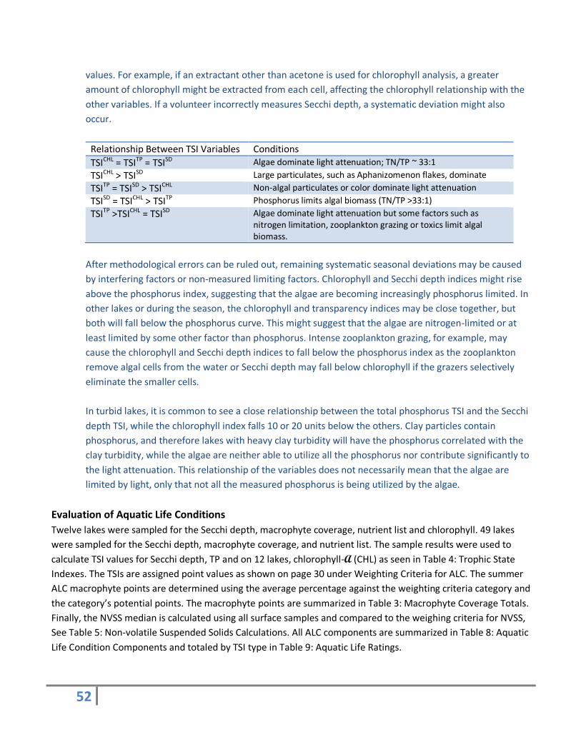
52
values. For example, if an extractant other than acetone is used for chlorophyll analysis, a greater
amount of chlorophyll might be extracted from each cell, affecting the chlorophyll relationship with the
other variables. If a volunteer incorrectly measures Secchi depth, a systematic deviation might also
occur.
Relationship Between TSI Variables Conditions
TSICHL = TSITP = TSISD Algae dominate light attenuation; TN/TP ~ 33:1
TSICHL > TSISD Large particulates, such as Aphanizomenon flakes, dominate
TSITP = TSISD > TSICHL Non-algal particulates or color dominate light attenuation
TSISD = TSICHL > TSITP Phosphorus limits algal biomass (TN/TP >33:1)
TSITP >TSICHL = TSISD Algae dominate light attenuation but some factors such as nitrogen limitation, zooplankton grazing or toxics limit algal biomass.
After methodological errors can be ruled out, remaining systematic seasonal deviations may be caused
by interfering factors or non-measured limiting factors. Chlorophyll and Secchi depth indices might rise
above the phosphorus index, suggesting that the algae are becoming increasingly phosphorus limited. In
other lakes or during the season, the chlorophyll and transparency indices may be close together, but
both will fall below the phosphorus curve. This might suggest that the algae are nitrogen-limited or at
least limited by some other factor than phosphorus. Intense zooplankton grazing, for example, may
cause the chlorophyll and Secchi depth indices to fall below the phosphorus index as the zooplankton
remove algal cells from the water or Secchi depth may fall below chlorophyll if the grazers selectively
eliminate the smaller cells.
In turbid lakes, it is common to see a close relationship between the total phosphorus TSI and the Secchi
depth TSI, while the chlorophyll index falls 10 or 20 units below the others. Clay particles contain
phosphorus, and therefore lakes with heavy clay turbidity will have the phosphorus correlated with the
clay turbidity, while the algae are neither able to utilize all the phosphorus nor contribute significantly to
the light attenuation. This relationship of the variables does not necessarily mean that the algae are
limited by light, only that not all the measured phosphorus is being utilized by the algae.
Evaluation of Aquatic Life Conditions
Twelve lakes were sampled for the Secchi depth, macrophyte coverage, nutrient list and chlorophyll. 49 lakes
were sampled for the Secchi depth, macrophyte coverage, and nutrient list. The sample results were used to
calculate TSI values for Secchi depth, TP and on 12 lakes, chlorophyll-A (CHL) as seen in Table 4: Trophic State
Indexes. The TSIs are assigned point values as shown on page 30 under Weighting Criteria for ALC. The summer
ALC macrophyte points are determined using the average percentage against the weighting criteria category and
the category’s potential points. The macrophyte points are summarized in Table 3: Macrophyte Coverage Totals.
Finally, the NVSS median is calculated using all surface samples and compared to the weighing criteria for NVSS,
See Table 5: Non-volatile Suspended Solids Calculations. All ALC components are summarized in Table 8: Aquatic
Life Condition Components and totaled by TSI type in Table 9: Aquatic Life Ratings.
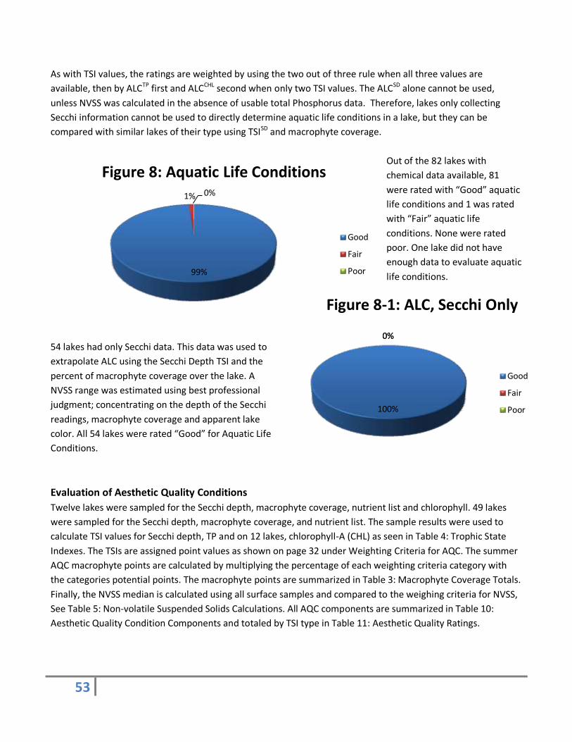
53
As with TSI values, the ratings are weighted by using the two out of three rule when all three values are
available, then by ALCTP first and ALCCHL second when only two TSI values. The ALCSD alone cannot be used,
unless NVSS was calculated in the absence of usable total Phosphorus data. Therefore, lakes only collecting
Secchi information cannot be used to directly determine aquatic life conditions in a lake, but they can be
compared with similar lakes of their type using TSISD and macrophyte coverage.
Out of the 82 lakes with
chemical data available, 81
were rated with “Good” aquatic
life conditions and 1 was rated
with “Fair” aquatic life
conditions. None were rated
poor. One lake did not have
enough data to evaluate aquatic
life conditions.
54 lakes had only Secchi data. This data was used to
extrapolate ALC using the Secchi Depth TSI and the
percent of macrophyte coverage over the lake. A
NVSS range was estimated using best professional
judgment; concentrating on the depth of the Secchi
readings, macrophyte coverage and apparent lake
color. All 54 lakes were rated “Good” for Aquatic Life
Conditions.
Evaluation of Aesthetic Quality Conditions
Twelve lakes were sampled for the Secchi depth, macrophyte coverage, nutrient list and chlorophyll. 49 lakes
were sampled for the Secchi depth, macrophyte coverage, and nutrient list. The sample results were used to
calculate TSI values for Secchi depth, TP and on 12 lakes, chlorophyll-A (CHL) as seen in Table 4: Trophic State
Indexes. The TSIs are assigned point values as shown on page 32 under Weighting Criteria for AQC. The summer
AQC macrophyte points are calculated by multiplying the percentage of each weighting criteria category with
the categories potential points. The macrophyte points are summarized in Table 3: Macrophyte Coverage Totals.
Finally, the NVSS median is calculated using all surface samples and compared to the weighing criteria for NVSS,
See Table 5: Non-volatile Suspended Solids Calculations. All AQC components are summarized in Table 10:
Aesthetic Quality Condition Components and totaled by TSI type in Table 11: Aesthetic Quality Ratings.
99%
1% 0%
Figure 8: Aquatic Life Conditions
Good
Fair
Poor
100%
0% 0%
Figure 8-1: ALC, Secchi Only
Good
Fair
Poor
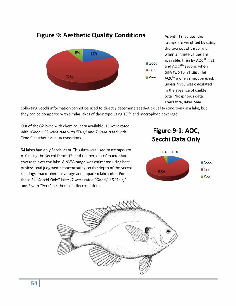
54
As with TSI values, the
ratings are weighted by using
the two out of three rule
when all three values are
available, then by AQCTP first
and AQCCHL second when
only two TSI values. The
AQCSD alone cannot be used,
unless NVSS was calculated
in the absence of usable
total Phosphorus data.
Therefore, lakes only
collecting Secchi information cannot be used to directly determine aesthetic quality conditions in a lake, but
they can be compared with similar lakes of their type using TSISD and macrophyte coverage.
Out of the 82 lakes with chemical data available, 16 were rated
with “Good,” 59 were rate with “Fair,” and 7 were rated with
“Poor” aesthetic quality conditions.
54 lakes had only Secchi data. This data was used to extrapolate
ALC using the Secchi Depth TSI and the percent of macrophyte
coverage over the lake. A NVSS range was estimated using best
professional judgment; concentrating on the depth of the Secchi
readings, macrophyte coverage and apparent lake color. For
these 54 “Secchi Only” lakes, 7 were rated “Good,” 45 “Fair,”
and 2 with “Poor” aesthetic quality conditions.
19%
72%
9%
Figure 9: Aesthetic Quality Conditions
Good
Fair
Poor
13%
83%
4%
Figure 9-1: AQC, Secchi Data Only
Good
Fair
Poor
55
Summary For many decades, lakes have been classified according to their trophic state. A eutrophic lake has high nutrients
and high plant growth. An oligotrophic lake has low nutrient concentrations and low plant growth. Mesotrophic
lakes fall between eutrophic and oligotrophic lakes. While lakes may be lumped into a few trophic classes, each
lake has a unique set of attributes that create its trophic state.
Three main factors contribute to the trophic state of a lake; rate of nutrient supply, climate, and shape of the
lake basin. The rate of nutrient supply is directly affected by the soils, vegetation and human land uses and
management practices in a lake’s watershed. The climate factors include the amount of sunlight a lake receives,
temperature and precipitation. Another important climate related factor is a lake’s turnover time and water
retention time. Finally, the shape of a lake basin affects how the other two factors interact. Basin morphology
factors include lake volume, depth, surface area and sized of its watershed.
Trophic status is a useful means of classifying lakes and describing lake processes in terms of the productivity of
the system. Basins with infertile soils release relatively little nitrogen and phosphorus leading to less productive
lakes, classified as oligotrophic or mesotrophic. Watersheds with rich organic soils, or agricultural regions
enriched with fertilizers, yield much higher nutrient loads, resulting in more productive, eutrophic (even hyper-
eutrophic) lakes.
The concept of lake aging has been interpreted by some as an inevitable and irreversible process whereby a lake
eventually "dies." In fact, many oligotrophic lakes have persisted as such since the last glaciation. Changes in
climate and watershed vegetation seem to have both increased and decreased lake productivity over this
period. Some lakes probably experienced high rates of photosynthesis fairly soon after glacial retreat and then
became less productive until recent times. It is also possible that water sources for some lakes have changed
over the past thousands of years through diversions of stream flow, for example. In such cases water supplies to
a lake (and therefore nutrient supplies) could have changed, leading to changes in the lake's productivity.
Lakes may undergo cultural eutrophication by accelerating their natural rate of nutrient inflow. This occurs
through poor management of the watershed and introduction of human wastes through failing septic systems.
Such changes may occur over periods of only decades and are reversible if anthropogenic nutrient loading can
be controlled.
In Illinois, most of the problems associated with the direct discharge of domestic wastewater have been
successfully mitigated. Now the focus is on the much more difficult problem of controlling non-point sources
(NPS) of nutrient pollution such as agricultural drainage, storm water runoff, and inadequate on-site septic
systems. NPS pollution is particularly difficult to address because it is diffuse, not attributable to a small number
of polluters, and associated with fundamental changes in the landscape, such as agriculture, urbanization and
shoreline development.
Data from the Volunteer Lake Monitoring Program continues to show heavy loading of nutrients such as
Phosphorus, into Illinois lakes. Data for the eighty-two lakes with total Phosphorus values had a median range
56
of 0.003 mg/L to 0.462 mg/L. The lowest single value for total phosphorus was 0.003 mg/L and the highest was
1.02 mg/L. The water quality standard for Illinois surface water is 0.05 mg/L. Twenty-nine of the eighty-two
lakes were under the surface water standard for their median total phosphorus values, but that number falls to
twenty-one without at least one value over 0.05 mg/L.
Twenty-seven of the eighty-two lakes had some level of concern for suspended solids, though only one had high
levels and four others were of moderate concern.
Besides high nutrient loads in Illinois lakes, balancing macrophyte coverage appears to be the number one factor
between keeping aquatic life conditions favorable while maintaining aesthetic quality conditions for recreation.
Thirty-nine of the one-hundred thirty-seven lakes studied had good macrophyte coverage for supporting aquatic
life while maintaining good recreational use conditions as well.
There are a number of options for improving the water quality of a lake – from picking up litter to implementing
best management practices in the watershed. Best management practices have been developed for
construction, cropland, and forestry, as well as other similar land-use activities. Managers of lakes and streams
can focus their best management practices to control water runoff, erosion, nutrient loading and contaminant
loading. Table 13 contains a long list of best management practices with a set of priorities assigned from low to
high for agriculture, construction, urban runoff, hydrologic modification, resource extraction, groundwater, and
wetlands.
Grants Available to Control Nonpoint Source Pollution in Illinois
Grants are available to local units of government and other organizations to protect water quality in Illinois.
Projects must address water quality issues relating directly to nonpoint source pollution. Funds can be used for
the implementation of watershed management plans including the development of information and/or
education programs and for the installation of best management practices.
IEPA receives these funds through Section 319(h) of the Clean Water Act and administers the program within
Illinois. The maximum federal funding available is 60 percent. The program period is two years unless otherwise
approved. This is a reimbursement program.
Applications are accepted June 1 through August 1. If August 1 is a Saturday or Sunday, the deadline becomes
the prior Friday before 5 p.m. At this time, electronic submittals are not accepted. Please mail applications to:
(217)782-3362
Links for 319 Grants
Section 319 Request for Proposals
Section 319 Application
Section 319 Application Instructions
Section 319 Certifications and Grant Conditions
Illinois Environmental Protection Agency
Bureau of Water
Watershed Management Section
Nonpoint Source Unit
1021 North Grand Avenue East
P.O. Box 19276
Springfield, Illinois 62794-9276
57
References
Allum, M. 0., Glessner, R. E., and Gakstatter, J. H. 1977. An Evaluation of the National Eutrophication
Survey Data Working Paper No. 900. Corvallis Environmental Research Laboratory, Corvallis, Oregon,
National Eutrophication Survey, Office of Research and Development, U.S. Environmental Protection
Agency, GPO 699-440.
Carlson, R.E. 1977. A tropic state index for lakes. Volume 22; Issue 2, American Society of Limnology and
Oceanography, Pages 361-369.
Carson, R. and Simpson, J. 1996. A Coordinator’s Guide to Volunteer Lake Monitoring Methods. North
American Lake Management Society.
McComas, Steve 1993. Lake Smarts The First Lake Management Handbook, 4th Edition. Terrene Institute,
Alexandria, Virginia.
North American Lake Management Society and Terrene Institute 2001. Managing Lakes and Reservoirs
(3rd Edition).
Shaw, Byron. Mechenich, Christine, and Klessig, Lowell 2004. Understanding Lake Data (G3582).
University of Wisconsin Extension. Cooperative Extension Publishing Operations.
Taylor, J. W. ed. 1984. “The Acid Test.” Natural Resources Magazine. Wis. Dept. of Natural Resources. 40
pp.
USEPA, Criteria and Standards Division 1988 (EPA-440/5-88-002) The Lake and Reservoir Restoration
Guidance Manual, 1st Edition.
USEPA, Water Division 1993 (EPA-841-R-93-002) Fish and Fisheries Management in Lake And Reservoirs.
Technical Supplement to: The Lake and Reservoir Restoration Guidance Manual.
Wetzel, R. G. 2000. Limnological Analyses. (3rd Edition) Springer-Verlag.
Wetzel, R. G. 2001. Limnology Lake and River Ecosystems. (3rd Edition). Academic Press
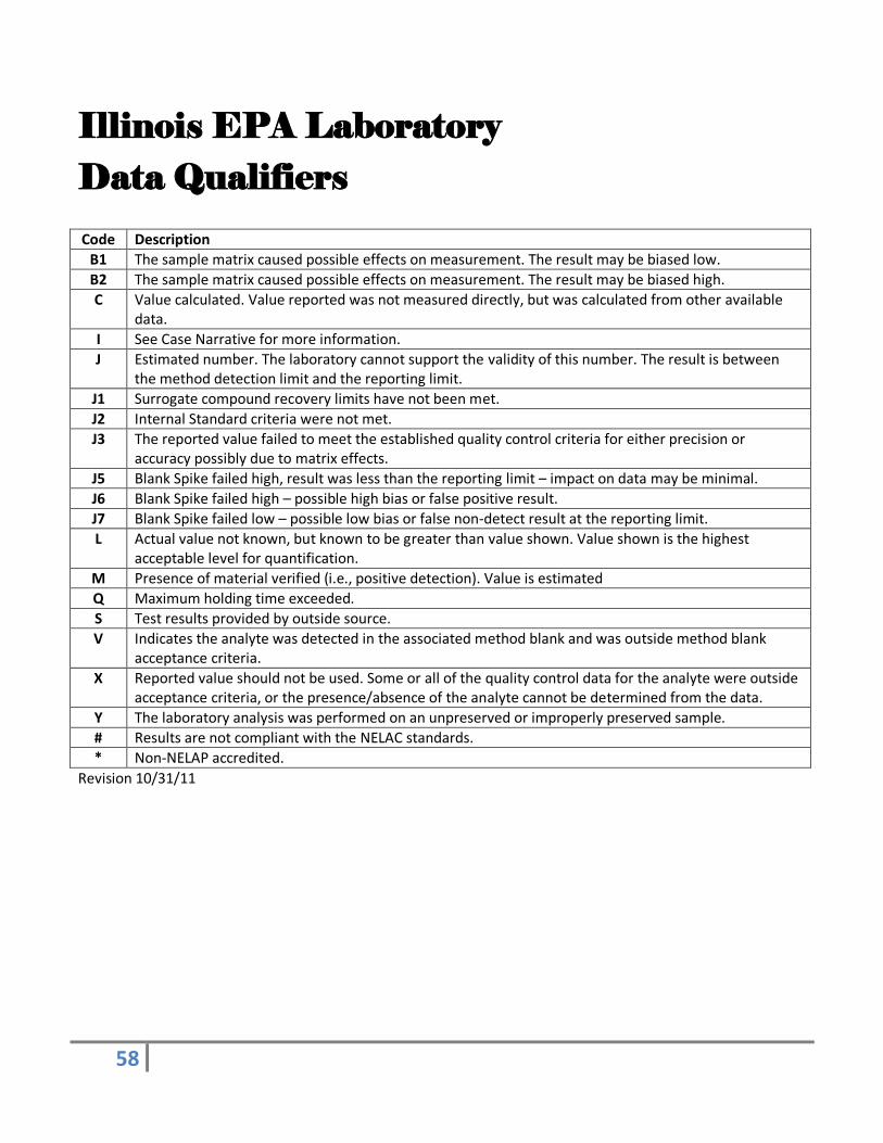
58
Illinois EPA Laboratory Data Qualifiers
Code Description
B1 The sample matrix caused possible effects on measurement. The result may be biased low.
B2 The sample matrix caused possible effects on measurement. The result may be biased high.
C Value calculated. Value reported was not measured directly, but was calculated from other available data.
I See Case Narrative for more information.
J Estimated number. The laboratory cannot support the validity of this number. The result is between the method detection limit and the reporting limit.
J1 Surrogate compound recovery limits have not been met.
J2 Internal Standard criteria were not met.
J3 The reported value failed to meet the established quality control criteria for either precision or accuracy possibly due to matrix effects.
J5 Blank Spike failed high, result was less than the reporting limit – impact on data may be minimal.
J6 Blank Spike failed high – possible high bias or false positive result.
J7 Blank Spike failed low – possible low bias or false non-detect result at the reporting limit.
L Actual value not known, but known to be greater than value shown. Value shown is the highest acceptable level for quantification.
M Presence of material verified (i.e., positive detection). Value is estimated
Q Maximum holding time exceeded.
S Test results provided by outside source.
V Indicates the analyte was detected in the associated method blank and was outside method blank acceptance criteria.
X Reported value should not be used. Some or all of the quality control data for the analyte were outside acceptance criteria, or the presence/absence of the analyte cannot be determined from the data.
Y The laboratory analysis was performed on an unpreserved or improperly preserved sample.
# Results are not compliant with the NELAC standards.
* Non-NELAP accredited.
Revision 10/31/11
59
Glossary of TermsAlgae: a group of photosynthetic eucaryotes that
are single celled, colonial, or filamentous aquatic
plants, often microscopic.
Algal bloom: A condition which occurs when
excessive nutrient levels and other physical and
chemical conditions facilitate rapid growth of algae.
Algal blooms may cause changes in water color. The
decay of the algal bloom may reduce dissolved
oxygen levels in the water.
Alkalinity: A measure of the capacity of water to
neutralize acids. It is a measure of the amount of
carbonates, bicarbonates, and hydroxide present in
water. Low alkalinity is the main indicator of
susceptibility to acid rain. Increasing alkalinity is
often related to increased algae productivity.
(Expressed as milligrams per liter (mg/L) of calcium
carbonate (CaCO3), or as microequivalents per liter
(μeq/l). 20 μeq/l = 1 mg/L of CaCO3.)
Ammonia: A form of nitrogen found in organic
materials and many fertilizers. It is the first form of
nitrogen released when organic matter decays. It
can be used by most aquatic plants and is therefore
an important nutrient. It converts rapidly to nitrate
(NO3 –) if oxygen is present. The conversion rate is
related to water temperature. Ammonia is toxic to
fish at relatively low concentrations in pH-neutral or
alkaline water. Under acid conditions, non-toxic
ammonium ions (NH4+) form, but at high pH values
the toxic ammonium hydroxide (NH4OH) occurs.
The water quality standard for indigenous aquatic
life is 0.1 mg/L of unionized ammonia. At a pH of 7
and a temperature of 68o Fahrenheit (20o Celsius),
the ratio of ammonium ions to ammonium
hydroxide is 250:1; at pH 8, the ratio is 26:1.
Anaerobic: Any process that can occur without
molecular oxygen; also applicable to organisms that
can survive without free oxygen.
Aquatic Invasive Species (AIS): AIS is a species that
is non-native to the ecosystem under consideration
and whose introduction causes or is likely to cause
economic or environmental harm or harm to
human health.
Aquatic invertebrates: Aquatic animals without an
internal skeletal structure such as insects, mollusks,
and crayfish.
Beneficial use: The uses of a water resource that
are protected by state laws called water quality
standards. Uses include aquatic life, recreation,
human consumption, and fish or wildlife habitat.
Benthic: Living in or on the bottom of a body of
water.
Benthos: Collectively, all organisms living in, on, or
near the bottom substrate in aquatic habitats
(examples are oysters, clams, burrowing worms).
Best management practices (BMPs): Management
practices (such as nutrient management) or
structural practices (such as terraces) designed to
reduce the quantities of pollutants — such as
sediment, nitrogen, phosphorus, and animal wastes
— that are washed by rain and snow melt from
lands into nearby receiving waters, such as lakes,
creeks, streams, rivers, estuaries, and ground water.
Biomass: The total quantity of plants and animals in
a lake. Measured as organisms or dry matter per
cubic meter, biomass indicates the degree of a lake
system’s eutrophication or productivity.
Blue-green algae: Algae which are often associated
with problem blooms in lakes. Some produce
chemicals toxic to other organisms, including
humans. They often form floating scum as they die.
Many can fix nitrogen (N2) from the air to provide
their own nutrient.
60
Chlorophyll: Green pigments essential to
photosynthesis.
Chlorophyll a: A green photosynthetic pigment
found in the cells of all algae and other plants. The
chlorophyll-a level in lake water is used to estimate
the concentration of planktonic algae in the lake.
Chlorophyll b: A type of chlorophyll found in green
algae and euglenoids. Both of these are good food
for zooplankton which is good fish food.
Chlorophyll c: A type of chlorophyll found in
diatoms and golden brown algae. Both of these are
good food for zooplankton which is good fish food.
Conductivity: The ability of water or other
substance to carry an electric current.
Color: Measured in color units that relate to a
standard. A yellow-brown natural color is associated
with lakes or rivers receiving wetland drainage.
Color also affects light penetration and therefore
the depth at which plants can grow.
Cultural Eutrophication: The enrichment of lakes
with nutrients (especially phosphorus) as a result of
human activity, resulting in an acceleration of the
natural ageing process of the lake.
Detritus: Fragments of plant material.
Diatoms: Any number of microscopic algae whose
cell walls consist of two box-like parts or valves and
contain silica.
Dinoflagellates: Unicellular biflagellate algae with
thick cellulose plates.
Dissolved Oxygen: Dissolved oxygen is the amount
of oxygen dissolved in the water. The DO
concentration in water is affected by the water
temperature, water quality, and other factors.
Epilmnion: the upper (usually warmer) circulated
zone of water in a temperature stratified lake.
Erosion: Wearing away of rock or soil by the gradual
detachment of soil or rock fragments by water,
wind, ice, and other mechanical, chemical, or
biological forces.
Euphotic: the zone of vertical light penetration in a
lake.
Eutrohic: water which are rich in plant nutrients
and capable of supporting high amounts of plant
and animal growth (Secchi transparency less than
6.6 feet and TSI 50 to 70).
Eutrophication: the lake aging process via nutrient
enrichment and sedimentation; both a natural and
human induced process.
Hypereutrophic: a lake with extreme level of
nutrients and nuisance plant growth, often as a
result of human activities (a TSI greater than 70).
Hypolimnion: the lower (usually cooler) non-
circulated zone of water in a temperature stratified
lake.
Invasive Species: An alien species whose
introduction does, or is likely to, cause economic or
environmental harm to human health.
Lake: A man-made impoundment or natural body of
fresh water of considerable size, whose open-water
and deep-bottom zones (no light penetration to
bottom) are large compared to the shallow-water
(shoreline) zone, which has light penetration to its
bottom.
Limnology: The scientific study of the life and
phenomena of lakes, ponds and streams.
Littoral Zone: The near shore shallow water zone of
a lake, where light penetrates to the bottom and
aquatic plants grow. Some shallow ponds are
entirely littoral.
Macroinvertebrate: Any nonvertebrate organism
that is large enough to be seen without the aid of a
microscope.
61
Macrophyte: water plants that are visable to the
unaided eye.
Mesotrophic: waters intermediate in eutrophy
between oligotrophic and eutrophic (Secchi
transparency 6.6 to 12.1 feet and TSI 40 to 50).
Metabolism: the sum of the physical and chemical
processes ongoing in all living things.
Methemoglobinemia: a condition brought on by
drinking water high in nitrates, that reduces the
ability of blood to carry oxygen and may also cause
respiratory problems. Infants are particularly at risk.
Native Species: A species naturally occurring of
originating in a geographical region or in a specific
ecosystem.
Nonpoint source (NPS) pollution: Unlike pollution
from industrial and sewage treatment plants, NPS
pollution comes from many diffuse sources. NPS
pollution is caused by rainfall or snowmelt moving
over and through the ground. As the runoff moves,
it picks up and carries away natural and human-
made pollutants, finally depositing them into lakes,
rivers, wetlands and even our underground sources
of drinking water. It has been determined that over
60 percent of the (national) documented water
pollution problem can be traced to nonpoint
sources.
Nutrients: Chemicals that are needed by plants and
animals for growth (e.g., nitrogen, phosphorus). In
water resources, if other physical and chemical
conditions are optimal, excessive amounts of
nutrients can lead to degradation of water quality
by promoting excessive growth, accumulation, and
subsequent decay of plants, especially algae. Some
nutrients can be toxic to animals at high
concentrations.
Oligotrophic: water with low concentrations of
plant nutrients and hence relatively low amounts of
plant and animal growth (Secchi transparency
greater than 12.1 feet and TSI less than 40).
Online Lakes Database: An online interface for
volunteer lake monitors to input their data into the
IEPA Lake’s Data Management System. It also
provides a means for all citizens to view current and
historical water quality information on monitored
lakes. Database currently contains only those lakes
sampled since 1999. Previous to 1999, all data may
be accessed through USEPA’s STORET.
pH: A measure of the acidic or basic (alkaline)
nature of water, relating to the number of hydrogen
ions. A pH of 7 is neutral. Acid waters are below 7;
alkaline waters are above 7.
Pheophytin: The dead chlorophyll of algal cells. Can
indicate when an algal bloom dies off.
Phosphorus: One of the major nutrients needed for
plant growth. Phosphorus is the critical nutrient for
algae growth in lake and ponds.
Photosynthesis: the process by which green plants
use sunlight, water, and carbon dioxide to produce
oxygen.
Plankton: Small organisms that float passively (or
swim weakly) in open water. The two groups of
plankton are: phytoplankton, also called algae; and
planktonic animals, also called zooplankton.
Pollutant: A contaminant that adversely alters the
physical, chemical, or biological properties of the
environment. The term includes nutrients,
sediment, pathogens, toxic metals, carcinogens,
oxygen-demanding materials, and all other harmful
substances. With reference to nonpoint sources,
the term is sometimes used to apply to
contaminants released in low concentrations from
many activities which collectively degrade water
quality. As defined in the federal Clean Water Act,
pollutant means dredged spoil, solid waste,
incinerator residue, sewage, garbage, sewage
sludge, munitions, chemical wastes, biological
materials, radioactive materials, heat, wrecked or
discarded equipment, rock, sand, cellar dirt, and
62
industrial, municipal, and agricultural waste
discharged into water.
Protoplasm: the living substance of in a cell
(includes the cytoplasm and nucleus).
Representative Site: generally is the deepest area
of the lake and is called Site 1.
Saturation: the maximum concentration that water
can hold (of any substance, in this case oxygen).
This is a function of temperature and pressure.
Secchi Disk Transparency: the depth in the water
column that an eight inch, black and white disk
disappears from view. Two or three time the Secchi
depth is the depth that sunlight can reach into the
water column and thereby support plant growth. A
healthy plant community is needed for animal (fish)
habitat within the lake.
Sediment: Particles and/or clumps of particles of
sand, clay, silt, and plant or animal matter carried in
water.
STORET: USEPA’s old national data storage
database; it is housed in a computer mainframe
system.
Stratification: The layering of water due to
differences in density. Water’s greatest density
occurs at 39o Fahrenheit (4o Celsius). As water
warms during the summer, it remains near the
surface while colder water remains near the
bottom. Wind mixing determines the thickness of
the warm surface water layer (epilimnion), which
usually extends to a depth of about 20 feet. The
narrow transition zone between the epilimnion and
cold bottom water (hypolimnion) is called the
thermocline.
Super-Saturation: a concentration of a substance
(in this case oxygen) above the maximum
concentration that water can hold at a given
temperature and pressure. This can happen when
temperature or pressure changes, or as a result of
biological activity.
Suspended solids: Suspended solids refer to small
solid particles which remain in suspension in water
as a colloid or due to the motion of the water. It is
used as one indicator of water quality
Thermal Stratification: As lake water is warmed in
the summer, the water in the deep pond or lake is
layered into three levels: 1) warmer (less dense)
epilimnion layer at the surface; 2) the thin
thermocline or transition layer; and 3) the cold and
deep hypolimnion layer.
Thermally Stratified: lake water often separates
into zones or layers by temperature difference.
Thermocline: the zone in a temperature-stratified
lake between the epilimnion and the hypolimnion,
also referred to as the “metalimnion.”
Total Phosphorus: A measure of all forms of
phosphorus (organic and inorganic) in water.
Total Suspended Solid (TSS): The weight of particles
that are suspended in water. Suspended solids in
water reduce light penetration in the water column,
can clog the gills of fish and invertebrates, and are
often associated with toxic contaminants because
organics and metals tend to bind to particles. Total
suspended solids are differentiated from total
dissolved solids by a standardized filtration process,
the dissolved portion passing through the filter.
Transparency: A measure of water clarity that, in
lakes and ponds, indirectly measures algal
productivity. Transparency is determined by the
depth at which a Secchi disk lowered into the water
column is no longer visible.
Trophic: A level of nutrition, nutrient enrichment
within a lake.
Trophic State Index (TSI): A simplified index of
biological productivity in lakes.
63
Turbidity: A measure of the amount of light
intercepted by a given volume of water due to the
presence of suspended and dissolved matter and
microscopic biota. Increasing the turbidity of the
water decreases the amount of light that
penetrates the water column. High levels of
turbidity are harmful to aquatic life.
Volatile suspended solids (VSS): That fraction of
suspended solids, including organic matter and
volatile inorganic salts, which will ignite and burn
when placed in an electric muffle furnace at 550 °C
for 15 minutes.
Watershed: A region or area divided by points of
high land that drains into a lake, stream, or river.
Watershed Based Plan: A watershed based plan is a
document designed to protect and improve water
quality by controlling nonpoint source pollution and
related water quality problems. Such plans provide
an integrated, holistic process to effectively and
efficiently protect, enhance and restore the
physical, chemical and biological integrity of water
resources within a defined hydrologic area
(watershed). Watershed based plans present
assessment and management information for a
geographically defined watershed, including the
analyses, actions, participants, and resources
related to development and implementation of the
plan. Watershed based plans should be consistent
with the nine minimum elements of watershed
based plan as defined by USEPA watershed based
plan guidance, the Chicago Metropolitan Agency for
Planning’s Guidance for Developing Watershed
Action Plans in Illinois, total maximum daily load
(TMDL) implementation plan requirements, and
current watershed planning principles.
Water quality standards: Established limits of
certain chemical, physical, and biological
parameters in a water body; water quality
standards are established for the different
designated uses of a water body.
Wetlands: Areas that are inundated or saturated by
surface or ground water at a frequency and
duration sufficient to support, and that under
normal circumstances do support, a prevalence of
vegetation typically adapted for life in saturated soil
conditions. Wetlands generally include swamps,
marshes, bogs, and similar areas.
Zooplankton: microscopic animals found in the
water of lakes and rivers.


