

Illiquidity, Portfolio Constraints, and
Diversification ∗
Min Dai, Hanqing Jin, and Hong Liu
This revision: March 5, 2008
∗Dai and Jin are from Department of Mathematics of National University of Singapore (NUS) andLiu is from the Olin Business School of Washington University in St. Louis. We thank Phil Dybvig,Bill Marshall, and the seminar participants at Washington University for helpful comments. Wethank Yifei Zhong for excellent research assistance. Authors can be reached at [email protected],[email protected], and [email protected]. Dai and Jin are partially supported by the NUS RMIresearch grant and the NUS academic research grant. All errors are ours.
Illiquidity, Portfolio Constraints, andDiversification
Extended Abstract
Mutual funds are often restricted to allocate certain percentages of fund assets tocertain securities that have different degrees of illiquidity. The coexistence of theserestrictions and asset illiquidity and the interactions among them are important forthe optimal trading strategy of a mutual fund. However, the existing literature ignoresthis coexistence and the interactions.
In this paper, we consider a fund that can trade a liquid stock and an illiquidstock that is subject to proportional transaction costs. The percentage of capitalallocated to the illiquid stock is restricted to remain between a lower bound andan upper bound. We use a novel approach to characterize the value function andto provide extensive analytical comparative statics on the optimal trading strategy.The optimal trading strategy for the illiquid stock is determined by the optimal buyboundary and the optimal sell boundary which are easy to compute numerically usinga penalty method. We also show the existence and uniqueness of the optimal tradingstrategy.
We also conduct numerical analysis on trading strategies, liquidity premium, anddiversification. Constantinides (1986) concludes that transaction costs only have asecond-order effect on liquidity premia. We find that the presence of portfolio con-straints can significantly magnify the effect of transaction costs on liquidity premiumand can make it more than a first-order effect. In addition, somewhat surprisingly,the liquidity premium can increase when constraints are less stringent. We show thateven for log preferences, the optimal trading strategy is nonmyopic with respect toportfolio constraints, in the sense that a constraint can affect current trading strat-egy even when it is not binding now. Correlation coefficient between the two stocksaffects the efficiency of diversification and thus can significantly alter the optimaltrading strategy in both stocks. We also examine the endogenous choice of the port-folio bounds. Our analysis shows that the optimal upper (lower) bound is increasing(decreasing) in transaction costs.
Journal of Economic Literature Classification Numbers: D11, D91, G11, C61.
Keywords: Illiquidity, Portfolio Constraints, Portfolio Selection, Transaction Costs
Mutual funds are often restricted to allocate certain percentages of fund assets to
certain securities that have different degrees of illiquidity. As stated in Almazan,
Brown, Carlson, and Chapman (2004), over 90% funds are restricted from buying-
on-margin and about 70% are prevented from short selling (see also, Clarke, de Silva,
and Thorley (2002)). These constraints are often specified in a funds prospectus and
differ across investment styles and country-specific regulations. For example, a small
cap fund may set a lower bound on its holdings of small cap stocks. U.S. stock funds
commonly state in their prospectus an obligation to hold less than 20% of non U.S.
stocks. In Switzerland, regulations require that at least two thirds of a fund’s assets
must be invested in the relevant geographical sectors (e.g., Switzerland, Europe) or
asset classes depending on the fund’s category. In France, regulations prevent bond
and money market funds from investing more than 10% in stocks. Mutual funds can
also face significant illiquidity in trading securities in some asset classes. Chalmers,
Edelen, and Kadlec (1999) conclude that annual trading costs for equity mutual funds
are large and exhibit substantial cross sectional variation, averaging 0.78% of fund
assets per year and having an inter-quartile range of 0.59%. Delib and Varma (2002)
find that transaction costs concerns can affect a fund’s permissible investment policy.
There is a large literature on optimal trading strategy of a mutual fund.1 However,
most of this literature does not consider the significant trading costs faced by funds or
the widespread portfolio constraints imposed upon mutual funds. As is well known,
the presence of transaction costs and portfolio constraints can have drastic impact
on the optimal trading strategy and thus the fund performance.2 The coexistence of
the portfolio constraints and asset illiquidity and the interactions among them are
1See, for example, Carpenter (2000), Basak, Pavlova and Shapiro (2006)2See, for example, Davis and Norman (1990), Cuoco (1997), Liu and Loewenstein (2002), and
Liu (2004).
1

important for the optimal trading strategy of a mutual fund. However, the existing
literature ignores this coexistence and the interactions.
In this paper, we consider a fund that can trade a liquid stock and an illiquid
stock that is subject to proportional transaction costs.3 The percentage of fund as-
sets allocated to the illiquid stock is restricted to remain between a lower bound
and an upper bound.4 Since the implied Hamilton-Jacobi-Bellman equation is highly
nonlinear and difficult to analyze, we convert the original problem into a double ob-
stacle problem which is much easier to analyze. Using this alternative approach, we
are able to characterize the value function and to provide many analytical compar-
ative statics on the optimal trading strategy. We show that there exists a unique
optimal trading strategy and the value function smooth except on a measure zero
set. The optimal trading strategy for the illiquid stock is determined by the optimal
buy boundary and the optimal sell boundary between which no transaction occurs.
Both the buy boundary and the sell boundary are monotonically decreasing in the
portfolio bounds. Intuitively, when a positive lower bound is raised, it is going to
bind for sure for the buy boundary when the time is close enough to the horizon.5
To partly make up for the extra transaction costs from the time T liquidation of this
over-investment, one also holds more at the buy boundary throughout the investment
horizon. On the other hand, when a binding upper bound is reduced, obviously one
needs to decrease the sell boundary. If the buy boundary remained the same, then
the no-transaction region would become narrower and the trading frequency would
3Vast majority of mutual funds are restricted from holding any significant amount of cash. Wetherefore simply assume that they can only invest in stocks. The less relevant case that allows thefund to hold a riskless asset can be similarly analyzed without much technical difficulty.
4Obviously, this implies that the percentage allocated to the liquid stock is also restricted.5This is because without a lower bound, the optimal buy boundary is always 0 with short enough
time to horizon, as shown in Section III..
2
increase. Therefore the buy boundary also shifts downward to save transaction costs
from frequent trading.
We find that the optimal buy (sell) boundary is monotonically decreasing (in-
creasing) in calendar time. As time passes and thus the remaining horizon shrinks, it
becomes less likely that the stock return over the remaining horizon can make up for
the transaction costs paid at transaction. Thus the fund increases the sell boundary
and lowers the buy boundary to decrease trading frequency.
We also conduct an extensive numerical analysis on trading strategies, liquidity
premium, and diversification. The above analytical results are useful for improving
the precision and robustness of the numerical procedure. Constantinides (1986) con-
cludes that transaction costs only have a second-order effect on liquidity premia. We
find that the presence of portfolio constraints can significantly magnify the effect of
transaction costs on liquidity premia and can make it more than a first-order effect.
Intuitively, the presence of constraints can force the fund to trade too frequently
and to substantially distort its trading strategy. In addition, surprisingly, the liquid-
ity premium can increase when constraints are less stringent. Lowering the binding
lower bound (and increasing the upper bound) decreases the optimal investment in
the illiquid stock and thus the value function becomes less sensitive to a change in the
expected return of the illiquid stock. Also, the value function in the presence of trans-
action costs increases less as the constraints become less and less binding. Therefore
it requires a greater reduction in the expected return (i.e., liquidity premium) in the
no transaction cost case to make the fund willing to face transaction costs.
Our numerical analysis shows that even for log preferences, the optimal trading
strategy is nonmyopic with respect to portfolio constraints, in the sense that con-
straints can affect current trading strategy even when they are not binding now.
3

Intuitively, even though the constraints are not binding now, they will for sure bind
when time to horizon becomes short enough. In anticipation of this future binding
of the constraints, the fund changes its current trading boundaries. Correlation co-
efficient between the two stocks affects the efficiency of diversification and thus can
significantly alter the optimal trading strategy in both the liquid stock and the illiquid
stock.
To partly address the endogeneity of the portfolio constraints, we also examine
the endogenous choice of the portfolio bounds by investors who have different risk
preferences from the fund managers.6 Our analysis show that the optimal upper
(lower) bound is increasing (decreasing) in transaction costs. This is because loosing
the constraints reduces transaction frequency and hence transaction costs.
This paper is closely related to two strands of literature: One on portfolio selection
with transaction costs and the other on portfolio selection with portfolio constraints.
The first strand of literature (e.g., Constantinides (1986), Davis and Norman (1990),
Liu and Loewenstein (2002), and Liu (2004)) finds that the presence of transaction
costs can dramatically change the optimal trading strategy and even a small trans-
action cost can significantly decrease the trading frequency. The second strand of
literature (e.g., Cvitanic and Karatzas (1992), Cuoco (1997), Cuoco and Liu (2000))
shows that portfolio constraints can also have large impact on the optimal trading
strategy. However, as far as we know, this is the first paper to consider the joint
impact of transaction costs and portfolio constraints. We find that the presence of
portfolio constraints can significantly magnify the impact of transaction costs on the
liquidity premium. In addition, the presence of transaction costs in general makes
6There are obviously other reasons for imposing constraints, e.g., different investment horizons,asymmetric information, etc.
4

the optimal trading strategy no longer myopic with respect to portfolio constraints.
The rest of the paper is organized as follows. In Section I., we describe the model.
We solve the first benchmark case without transaction costs in Section II.. We solve
the second benchmark case with transaction costs but without portfolio constraints
in Section III.. Section IV. provides a verification theorem and an analysis of the
main problem. In Section V. we conduct an extensive numerical analysis. Section VI.
concludes. All the proofs are contained in the Appendix.
I. The Model
We consider a fund manager who has a finite horizon T ∈ (0,∞) and maximizes his
constant relative risk averse (CRRA) utility from terminal wealth.7 The fund can
invest in two assets. One is a liquid risky asset (“the liquid stock,” e.g., a large cap
stock, S&P index) whose price process SLt evolves as 8
dSLt
SLt
= µLdt + σLdBLt, (1)
where µL and σL > 0 are both constants and BLt is a one-dimensional Brownian
motion. The other is an illiquid risky asset (“the illiquid stock,” e.g., a small cap
stock, an emerging market portfolio). The investor can buy the illiquid stock at the
ask price SAIt = (1 + θ)SIt and sell the stock at the bid price SB
It = (1− α)SIt, where
θ ≥ 0 and 0 ≤ α < 1 represent the proportional transaction cost rates and SIt follows
7This form of utility function is consistent with a linear fee structure predominantly adopted bymutual fund companies and is also commonly used in the literature (e.g., Carpenter (2000), Basak,Pavlova, and Shapiro (2006)). As in Huang and Liu (2007), generalization to the class of hyperbolicabsolute risk averse utility is straightforward.
8Extension to a case with a risk-free asset and/or multiple liquid assets is trivial and does notchange any of the qualitative results. Since most funds are prohibited from making any significantamount of risk-free investment, we assume that the fund cannot hold any risk-free asset. In fact, wehave numerically solved the case where investment in the risk free asset is allowed but the fractionof wealth invested in the risk free asset is restricted to be small in addition to the constraints on theilliquid asset holdings, all the qualitative results hold.
5

the process
dSIt
SIt
= µIdt + σIdBIt, (2)
where µI and σI > 0 are both constants and BIt is another one-dimensional Brownian
motion that has a correlation of ρ with BLt with |ρ| < 1.9
When α + θ > 0, the above model gives rise to equations governing the evolution
of the dollar amount invested in the liquid stock, xt, and the dollar amount invested
in the illiquid stock, yt:
dxt = µLxtdt + σLxtdBLt − (1 + θ)dIt + (1− α)dDt, (3)
dyt = µIytdt + σIytdBIt + dIt − dDt, (4)
where the processes D and I represent the cumulative dollar amount of sales and
purchases of the illiquid stock, respectively. D and I are nondecreasing and right
continuous adapted processes with D(0) = I(0) = 0.
Let Wt = xt + yt be the fund’s wealth (on paper) at time t. The fund is subject
to the following exogenously given constraints on its trading strategy:10
b ≤ yt
Wt
≤ b, ∀t ≥ 0, (5)
where −1θ≤ b < b ≤ 1
αare constants.11 These constraints restrict the fraction of
wealth (on paper) that must be invested in the illiquid asset and imply that the fund
9The case with perfect correlation is straightforward to analyze, but needs a separate treatment.We thus omit it to save space.
10Because of possible misalignment of interests between the fund manager and the investor (e.g.,different risk tolerance, different investment horizons, different view of asset characteristics, etc.),the investor may impose portfolio constraints on the trading strategy of the fund. See Almazanet. al. (2004) for more details on why many mutual fund managers are constrained. In this paperwe focus on the case where this constraint is exogenously given and do not consider the optimalcontracting issue. This serves as a foundation toward examining the optimal contracting problemin the presence of transaction costs and endogenous portfolio constraints. Later in this paper, weillustrate the choice of optimal constraints using numerical examples.
11Similar arguments to those in Cuoco and Liu (2000) imply that the margin requirement for theone-stock case is a special case of this constraint. So our model can also be used to study the effectof margin requirement in the presence of transaction costs.
6

is always solvent after liquidation, i.e., the liquidation wealth12
Wt ≥ 0, ∀t ≥ 0, (6)
where
Wt = xt + (1− α)y+t − (1 + θ)y−t . (7)
Let x0 and y0 be the given initial positions in the liquid stock and the illiquid
stock respectively. We let Θ(x0, y0) denote the set of admissible trading strategies
(D, I) such that (3), (4), and (5).
The fund manager’s problem is then13
sup(D,I)∈Θ(x0,y0)
E [u(WT )] , (8)
where the utility function is given by
u(W ) =W 1−γ − 1
1− γ
and γ > 0 is the constant relative risk aversion coefficient. This specification allows
us to obtain the corresponding results for the log utility case by letting γ approach
1. Implicitly, we assume that the performance evaluation or incentive fee structure
depends on the wealth on paper instead of the liquidation wealth. This is consistent
with common industry practice and avoids trading strategies that lead to liquidation
on the terminal date.
12Choosing the wealth on paper in (5) instead of the wealth after liquidation (as defined in (7) asthe denominator is consistent with common industry practice. Switching the choice does not affectour main results.
13It can be shown that as long as b > b, there exist feasible strategies and this problem is wellposed. The proof of this claim is omitted to save space.
7
II. Optimal Policies without Transaction Costs
For purpose of comparison, let us first consider the case without transaction costs
(i.e., α = θ = 0). In this case, the fund manager’s problem at time t becomes
J(W, t) ≡ supπL,πI
Et [u(WT )|Wt = W ] , (9)
subject to the self financing condition
dWs = (1− πIs) WsµLds + (1− πIs) WsσLdBLs + πIsWsµIds + πIsWsσIdBIs, ∀s ≥ t,
(10)
and the portfolio constraint (5), where πIs represents the fraction of wealth invested
in the illiquid stock.
Let πMI (“Merton line”) be the optimal fraction of wealth invested in the illiquid
stock in the unconstrained case in the absence of transaction costs. Then it can be
shown that
πMI =
µI − µL + γσL (σL − ρσI)
γ (σ2L + σ2
I − 2ρσLσI). (11)
We summarize the main result for this case of no transaction costs in the following
theorem.
Theorem 1 Suppose that α = θ = 0. Then the optimal trading policy is given by
π∗I =
b if πMI ≥ b
πMI if b < πM
I < bb if πM
I ≤ b, π∗L = 1− π∗I
and the value function is
J(W, t) =
(eη(T−t)W
)1−γ − 1
1− γ,
where
η = µIπ∗I + µL (1− π∗I )−
1
2γ
[σ2
Iπ∗2I + σ2
L (1− π∗I )2 + 2ρσIσLπ∗I (1− π∗I )
].
8

Proof: see Appendix.
Theorem 1 implies that the optimal fractions of wealth invested in each asset are
time and horizon independent. In addition, the investor is myopic with respect to the
constraints even for a nonlog preference. Specifically, the optimal fraction is equal to
a bound if and only if the unconstrained optimal fraction violates the bound. We will
show that in the presence of transaction costs, the investor will no longer be myopic
even with a log preference.
III. The Transaction Cost Case without Constraints
In the case where α + θ > 0 , the problem is considerably more complicated. In this
section, we consider the unconstrained case first. In this case, the investor’s problem
at time t becomes
V (x, y, t) ≡ sup(D,I)∈Θ(x,y)
Et [u(WT )|xt = x, yt = y] (12)
with b = −1θ
and b = 1α. Under regularity conditions on the value function, we have
the following HJB equation:
max(Vt + L V, (1− α)Vx − Vy,−(1 + θ)Vx + Vy) = 0,
with the boundary conditions
(1− α)Vx − Vy = 0 ony
x + y=
1
α, (1 + θ)Vx − Vy = 0 on
y
x + y= −1
θ,
and the terminal condition
V (x, y, T ) =(x + y)1−γ − 1
1− γ,
where
L V =1
2σ2
Iy2Vyy +
1
2σ2
Lx2Vxx + ρσIσLxyVxy + µIyVy + µLxVx
9
As we show later, the HJB equation implies that the solvency region for the illiquid
stock
S =
(x, y) : x + (1− α)y+ − (1 + θ)y− > 0
at each point in time splits into a “Buy” region (BR), a “No-transaction” region
(NTR), and a “Sell” region (SR), as in Davis and Norman (1990).
The homogeneity of the utility function u and the fact that Θ(βx, βy) = βΘ(x, y)
for all β > 0 imply that V + 11−γ
is concave in (x, y) and homogeneous of degree 1−γ
in (x, y) [cf. Fleming and Soner (1993), Lemma VIII.3.2]. This homogeneity implies
that
V (x, y, t) ≡ (x + y)1−γ ϕ
(y
x + y, t
)− 1
1− γ, (13)
for y > 0 and some function ϕ : (α− 1,∞)× [0, T ] → IR. Let
π =y
x + y(14)
denote the fraction of wealth invested the illiquid stock. The homogeneity property
then implies that Buy, No-transaction, and Sell regions can be described by two
functions of time πI(t) and πI(t). The Buy region BR corresponds to π ≤ πI(t), the
Sell region SR to π ≥ πI(t), and the No-Transaction region NTR to πI(t) < π < πI(t).
A time snapshot of these regions is depicted in Figure 1. As we show later, the
optimal trading strategy in the illiquid stock is to transact a minimum amount to
keep the ratio πt in the optimal no-transaction region. Therefore the determination
of the optimal trading strategy in the illiquid stock reduces to the determination of
the optimal no-transaction region. In contrast to the no-transaction cost case, the
optimal fractions of the liquidated wealth invested in both the illiquid and the liquid
stocks change stochastically, since πt varies stochastically due to no transaction in
NTR.
10

ySELL
No-Transaction
BUY
x=z y
x
x=z y
0
Solvency Linex=-(1- )y
x=-(1+ )y
Solve
ncy L
ine
_
_
α
θ
Figure 1: The Solvency Region
Using (13), the HJB equation simplifies into:
max(ϕt + L1ϕ,− (1− απ) ϕπ − α (1− γ) ϕ, (1 + θπ) ϕπ − θ (1− γ) ϕ) = 0,
with the terminal condition
ϕ(π, T ) =1
1− γ,
where
L1ϕ =1
2β1π
2 (1− π)2 ϕππ+(β2 − γβ1π) π (1− π) ϕπ+(1− γ)
(β3 + β2π − 1
2γβ1π
2
)ϕ,
β1 = σ2I + σ2
L − 2ρσIσL,
β2 = µI − µL + γσL (σL − ρσI) , (15)
β3 = µL − 1
2γσ2
L.
11
The nonlinearity of this HJB equation and the time-varying nature of the free
boundaries make it difficult to solve directly. Instead, as in Dai and Yi (2006), we
transform the above problem into a double obstacle problem, which is much easier to
analyze. All the analytical results in this paper are obtained through this approach.
Theorem 2 in the next section shows the existence and the uniqueness of the
optimal trading strategy in the case with portfolio constraints and also applies to
the unconstrained case by choosing constraints that never bind. It also ensures the
smoothness of the value function except for a set of measure zero.
Before we proceed further, we make the following assumption to simplify analysis.
Assumption 1 α > 0, θ > 0, and − 1α
+ 1 < πMI < 1
θ+ 1.
Assuming the transaction costs for both purchases and sales to be positive reflects
the common industry practice. Since α and θ are typically small (e.g., 0.05), the
assumption that − 1α
+ 1 < πMI < 1
θ+ 1 is almost without loss of generality.
Let πI(t) be the optimal sell boundary and πI(t) be the optimal buy boundary
in the (π, W ) plane. Then we have the following properties for the no-transaction
boundaries in the (π,W ) plane.
Proposition 1 Let πMI is as defined in (11). Under Assumption 1, we have ∀t ∈
[0, T ],
1. for the sell boundary, there exists t < T such that
1
α= πI(s) ≥ πI(t) ≥ πM
I
1− α (1− πMI )
, for any t and all s > t;
2. for the buy boundary, there exists t < T such that
−1
θ= πI(s) ≤ πI(t) ≤
πMI
1 + θ (1− πMI )
, for any t and all s > t.
12

Proof: see Appendix.
This proposition shows that both the buy boundary and the sell boundary become
the solvency line when the investment horizon is short enough. In addition, if πMI ∈
(0, 1), then the width of the NTR is bounded below by
(θ + α)(1− πMI )πM
I
(1− α (1− πMI ))(1 + θ (1− πM
I )).
Let
β4 = µI − µL − γσI (σI − ρσL) ,
t0 = T − 1
β2
log (1− µ) , t1 = T − 1
β4
log (1− µ) , (16)
t0 = T − 1
β2
log (1 + θ) , t1 = T − 1
β4
log (1 + θ) . (17)
Proposition 2 Under Assumption 1, we have:
1. If πMI < 0, then πI(t) < 0 for all t and πI(t) is below 0 for t < t0, between 0
and 1 for t ∈ [t0, t1], and above 1 for t > t1; In addition, πI(t) is increasing in t for
t > t0.
2. If 0 < πMI < 1, then πI(t) is between 0 and 1 for t < t0 and below 0 for t ≥ t0;
πI(t) is between 0 and 1 for t < t1 and above 1 for t ≥ t1; In addition, πI(t) is
decreasing in t for t > t0 and πI(t) is increasing in t for t > t1.
3. If πMI > 1, then πI(t) > 1 for all t, and πI(t) is above 1 for t < t1, between 0
and 1 for t ∈ [t1, t0], and below 0 for t > t0; In addition, πI(t) is decreasing in t for
t > t1.
4. If πMI = 0, then πI(t) < 0 and πI(t) > 0 for all t, and πI(t) = πI(t) = 0
if T = ∞. Similarly, if πMI = 1, then πI(t) < 1 and πI(t) > 1 for all t, and
πI(t) = πI(t) = 1 if T = ∞. In addition, if πMI = 0 or πM
I = 1, then πI(t) is
decreasing in t and πI(t) is increasing in t for t ∈ [0, T ].
13
Proof: see Appendix.
Proposition 2 shows the presence of transaction costs can make a long position
optimal when a short position is optimal in the absence of transaction costs and
vice versa. For example, Part 1 of Proposition 1 shows that if the time to horizon
is short (i.e., < T − t0), then the sell boundary will be always positive even if it is
optimal to short the illiquid asset in the absence of transaction costs. This implies
that if the fund starts with a large position in the illiquid asset, then the fund will
only sell a part its position and optimally choose to keep a long position in it. This
is because trading the large long position into a short position would incur large
transaction costs. Similar results also hold when it is optimal to long in the absence
of transaction costs.
We conjecture that the optimal buy boundary is always decreasing in time and
the optimal sell boundary is always increasing in time. Unfortunately, we can only
show this when πMI = 0 or πM
I = 1. However, for other cases, we are able to show
this property when the horizon is short enough. For example, Part 2 implies that this
monotonicity holds when t > max(t1, t0).
Propositions 1 and 2 imply that in the absence of position limits, the portfolio
chosen by the fund can be far from the optimal portfolio that is optimal without
transaction costs. This large deviation is suboptimal for investors with longer horizons
and therefore it may be one of the reasons for investors to impose position limits.
14

IV. The Transaction Cost Case With Portfolio Con-
straints
Now we examine the case with both transaction costs and portfolio constraints. In
this case, the investor’s problem at time t can be written as
V c(x, y, t) ≡ sup(D,I)∈Θ(x,y)
E [u(WT )|xt = x, yt = y] (18)
with b ≤ ys/(xs + ys) ≤ b for all T ≥ s ≥ t.
Under regularity conditions on the value function, we have the following HJB
equation:
max(V ct + L V c, (1− α)V c
x − V cy ,−(1 + θ)V c
x + V cy ) = 0, (19)
with the boundary conditions14
(1− α)V cx − V c
y = 0 ony
x + y= b, (1 + θ)V c
x − V cy = 0 on
y
x + y= b,
and the terminal condition
V c(x, y, T ) =(x + y)1−γ − 1
1− γ.
The following verification theorem shows the existence and the uniqueness of the
optimal trading strategy. It also ensures the smoothness of the value function except
for a set of measure zero.
Theorem 2 (i) The HJB equation (19) admits a unique viscosity solution, and
the value function is the viscosity solution.
14It should be pointed out that the boundary conditions should be slightly modified when b = 0,or b = 1. For example, if πM
I > 0, we then infer from Proposition 2 that π = 0, t0 < t < T belongsto NTR, and the corresponding value function there
V c(x, 0, t) = E [u (xT ) |xt = x] =x1−γe(1−γ)(µL− 1
2 γσ2L)(T−t) − 1
1− γ, for t0 ≤ t < T,
which is the boundary condition at b for t ∈ [t0, T ) if b = 0.
15
(ii) The value function is C2,2,1 in (x, y, t) : x + (1 − α)y+ − (1 + θ)y− > 0, b <
y/(x + y) < b, 0 ≤ t < T \ (y = 0 ∪ x = 0).
Proof: see Appendix.
Similar to πI(t) and πI(t), let πcI(t; b, b) and πc
I(t; b, b) be respectively the optimal
sell and buy boundaries in the (π, W ) plane in the presence of constraints.
We have the following proposition on the properties of the optimal no-transaction
boundaries in the (π,W ) plane.
Proposition 3 Under Assumption 1, we have
1. for the sell boundary, there exists tb < T such that
b = πcI(s; b, b) ≥ πc
I(t; b, b) ≥ max
(min
(πM
I
1− α (1− πMI )
, b
), b
), for any t and all s > tb;
(20)
2. for the buy boundary, there exists tb < T such that
min
(max
(πM
I
1 + θ (1− πMI )
, b
), b
)≥ πc
I(t; b, b) ≥ πcI(s; b, b) = b, for any t and all s > tb.
(21)
Proof: The proof is similar to that of Proposition 1.
Corollary 1 Under Assumption 1,
1. ifπM
I
1−α(1−πMI )
≥ b, then πcI(t; b, b) = b for all t ∈ [0, T ];
2. ifπM
I
1+θ(1−πMI )
≤ b, then πcI(t; b, b) = b for all t ∈ [0, T ].
As stated in Corollary 1, these results imply that if the adjusted Merton line is
higher than the upper bound, then the sell boundary becomes flat throughout the
horizon and that if the adjusted Merton line is lower than the lower bound b , then
16

the buy boundary becomes flat throughout the horizon. Proposition 3 also shows that
the buy (sell) boundary remain flat at the lower bound b (upper bound b) when the
remaining horizon is short enough irrespective of the level of the Merton line. This
is the same as in the unconstrained case.
Proposition 4 Under Assumption 1, we have:
1. Both πcI(t; b, b) and πc
I(t; b, b) are increasing in b and b for all t ∈ [0, T ];
2. If b > 0, then the upper bound does not affect the sell/buy boundary that is below
0; If b > 1, then the upper bound does not affect the sell/buy boundary that is
below 1;
3. If b < 0, then the lower bound does not affect the sell/buy boundary that is above
0; If b < 1, then the lower bound does not affect the sell/buy boundary that is
above 1;
Proof: see Appendix.
Part 1 of Proposition 4 suggests that both the sell boundary and the buy boundary
at any point in time shift upward as the lower bound or the upper bound increases.
Intuitively, when a positive lower bound is raised, it is going to bind for sure for the
buy boundary when the time is close enough to the horizon. To partly make up for
the extra transaction costs from the time T liquidation of this over-investment, one
also holds more at the buy boundary throughout the investment horizon. When a
binding upper bound is reduced, obviously one needs to decrease the sell boundary. If
the buy boundary remained the same, then the no-transaction region would become
narrower and the trading frequency would increase. Therefore the buy boundary also
shifts downward to save transaction costs from frequent trading.
17

Parts 2 and 3 of Proposition 4 suggest that the optimal boundaries in the each
of the three regions: π ≤ 0, 0 < π < 1, and π ≥ 1 are not affected by an
constraint that lies in a different region. Intuitively, this is because in NTR, the
position in the illiquid asset can never become levered if it is unlevered at time 0
and can never become negative if it is positive at time 0, i.e., the fraction of wealth
invested in the illiquid asset cannot cross the π = 1 line or the π = 0 line.
Proposition 5 Under Assumption 1, suppose b < 0 and b > 0. Then we have:
1. If πMI < 0, then πI(t) < 0 for all t and πI(t) is below 0 for t < t0, between 0
and min(b, 1) for t ≥ t0; In addition, πI(t) is increasing in t for t > t0.
2. If 0 < πMI < 1, then πI(t) is between 0 and min(b, 1) for t < t0 and below 0 for
t ≥ t0; πI(t) is between 0 and min(b, 1) for all t; In addition, πI(t) is decreasing
in t for t > t0.
3. If πMI ≥ 1, then πI(t) ≥ min(b, 1) for all t, and πI(t) is between 0 and min(b, 1)
for t ≤ t0, and below 0 for t > t0; In addition, πI(t) is decreasing in t for t > t0.
4. If πMI = 0, then πI(t) < 0 and πI(t) > 0 for all t, and πI(t) = πI(t) = 0 if
T = ∞. In addition, πI(t) is decreasing in t and πI(t) is increasing in t for
t ∈ [0, T ].
Proof: see Appendix.
Proposition 6 Under Assumption 1, suppose 0 ≤ b < 1 and b > 1. Then we have:
1. If πMI ≤ 0, then πI(t) = b for all t, and πI(t) is between b and 1 for t ≥ t1, and
above 1 for t > t1; In addition, πI(t) is increasing in t for t > t1.
18

2. If 0 < πMI < 1, then πI(t) is between b and 1 for all t and πI(t) is between b
and 1 for t < t1 and above 1 for t ≥ t1; In addition, πI(t) is increasing in t for
t > t1.
3. If πMI > 1, then πI(t) > 1 for all t, and πI(t) is above 1 for t < t1, between b
and 1 for t > t1; In addition, πI(t) is decreasing in t for t > t1.
4. If πMI = 1, then πI(t) < 1 and πI(t) > 1 for all t, and πI(t) = πI(t) = 1 if
T = ∞. In addition, πI(t) is decreasing in t and πI(t) is increasing in t for
t ∈ [0, T ].
Proof: see Appendix.
Propositions 5 and 6 shows similar results on the properties of the optimal trading
boundaries to those in Proposition 2. In particular, monotonicity patterns remain
the same in the presence of constraints for the two cases in these two propositions.
The only difference is that the portfolio constraints may be binding in some regions.
Interestingly, even when the portfolio constraints are binding, the times that optimal
boundaries cross 0 and 1 remain unchanged. For example, Part 1 of Proposition 6
suggests the time that the sell boundary reaches 1 (i.e., t1) is the same as that in the
unconstrained case.
V. Numerical Analysis
In this section, we conduct numerical analysis of the optimal trading strategy, the
diversification, and the liquidity premium. For this analysis we use the following
default parameter values: γ = 2, T = 5, µL = 0.06, σL = 0.20, µI = 0.11, σI = 0.25,
ρ = 0.2, α = 0.01, θ = 0.01, b = 0.60, and b = 0.80, which implies that the fraction
of wealth invested in the illiquid (small cap) stock is greater than that in the liquid
19

(large cap) stock. For a large cap fund, we set b = 0.10 and b = 0.30 so that the
fraction of wealth invested in the liquid (large cap) stock is greater than that in the
illiquid (small cap) stock. We use a higher expected return and a higher volatility
for the small cap stock than those for a large cap stock. We use a penalty method to
solve the HJB equations (see Dai, Kwok, and Zong (2007) for example).
In Figure 2, we plot πI against calendar time t for the constrained case (the solid
lines) and the unconstrained case (the dotted lines). The dashed line represents the
Merton line in the absence of transaction costs. Consistent with the theoretical re-
sults in the previous section, this figure shows that the buy boundary is monotonically
decreasing in time and the sell boundary are monotonically increasing in time. The
lower bound of 60% is binding throughout the investment horizon and therefore the
buy boundary becomes flat at 60% across all time. The sell boundary reaches the
upper bound of 80% at t = 4.74. In addition, compared to the unconstrained case,
the sell boundary before t = 3.98 is moved higher and the portion after t = 3.98 is
moved lower. Thus, the optimal trading strategy is not myopic in the sense that in
anticipation of the constraint becoming binding later, it is optimal to change the early
trading strategy. Intuitively, since the fund will be forced to sell some of the illiquid
stock later on and the buy boundary is forced to move higher than the unconstrained
case, the fund needs to increase the sell boundary early on to reduce transaction fre-
quency and transaction cost payment. The Merton line is flat through time, implying
that in the absence of transaction costs, it is optimal to keep a constant fraction
of wealth in the stock. In the presence of transaction costs, however, the optimal
fraction becomes a stochastic process.
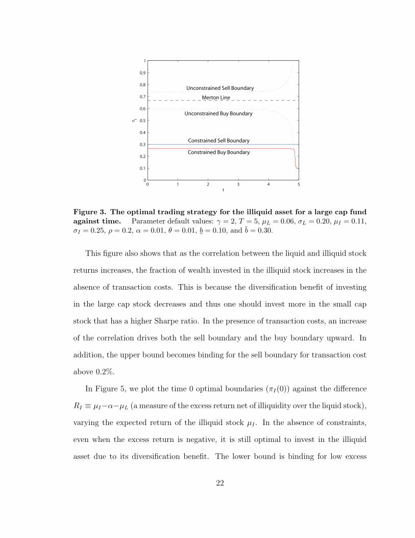
We present a similar figure (Figure 3) for the large cap fund case. In this case, both
the lower bound (10%) and the upper bound (30%) are tight constraints and the upper
20

0 1 2 3 4 50.5
0.55
0.6
0.65
0.7
0.75
0.8
0.85
t
πI
Constrained Sell Boundary
Unconstrained Sell Boundary
Merton Line
Constrained Buy Boundary
Unconstrained Buy Boundary
Figure 2. The optimal trading strategy for the illiquid asset for a small capfund against time. Parameter default values: γ = 2, T = 5, µL = 0.06, σL = 0.20,µI = 0.11, σI = 0.25, ρ = 0.2, α = 0.01, θ = 0.01, b = 0.60, and b = 0.80.
bound becomes so restrictive that the sell boundary becomes flat at 30% throughout
the horizon. The buy boundary also shifts downward significantly through most of the
horizon and only shifts upward towards the end of the horizon. In contrast to Figure
2, the Merton line is outside the optimal no transaction region for the constrained
case. These parameter values for the constraints can be reasonable for investors who
are more risk averse than the fund manager.
In Figure 4, we plot the time 0 optimal boundaries (πI(0)) against the transaction
cost rate α for several different cases. In the unconstrained case, as the transaction
cost rate increases, the buy boundary decreases and the sell boundary increases and
thus the no transaction region widens to decrease transaction frequency. In contrast,
the buy boundary in the presence of constraints first decreases and then stays at the
lower bound because the lower bound becomes binding. The binding lower bound
also drives up the sell boundary and makes it move up more for higher transaction
cost rates.
21
0 1 2 3 4 50
0.1
0.2
0.3
0.4
0.5
0.6
0.7
0.8
0.9
1
t
πI
Unconstrained Sell Boundary
Merton Line
Unconstrained Buy Boundary
Constrained Sell Boundary
Constrained Buy Boundary
Figure 3. The optimal trading strategy for the illiquid asset for a large cap fundagainst time. Parameter default values: γ = 2, T = 5, µL = 0.06, σL = 0.20, µI = 0.11,σI = 0.25, ρ = 0.2, α = 0.01, θ = 0.01, b = 0.10, and b = 0.30.
This figure also shows that as the correlation between the liquid and illiquid stock
returns increases, the fraction of wealth invested in the illiquid stock increases in the
absence of transaction costs. This is because the diversification benefit of investing
in the large cap stock decreases and thus one should invest more in the small cap
stock that has a higher Sharpe ratio. In the presence of transaction costs, an increase
of the correlation drives both the sell boundary and the buy boundary upward. In
addition, the upper bound becomes binding for the sell boundary for transaction cost
above 0.2%.
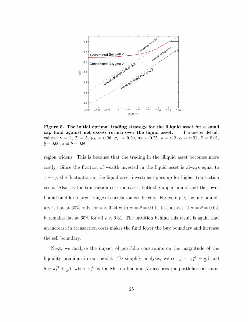
In Figure 5, we plot the time 0 optimal boundaries (πI(0)) against the difference
RI ≡ µI−α−µL (a measure of the excess return net of illiquidity over the liquid stock),
varying the expected return of the illiquid stock µI . In the absence of constraints,
even when the excess return is negative, it is still optimal to invest in the illiquid
asset due to its diversification benefit. The lower bound is binding for low excess
22

0 0.01 0.02 0.03 0.04 0.050.5
0.55
0.6
0.65
0.7
0.75
0.8
0.85
α
πI(0)
Constrained Sell ρ=0.2Unconstrained Sell ρ=0.2
Constrained Sell ρ=0.5
Unconstrained Buy ρ=0.2
Constrained Buy ρ=0.2
Constrained Buy ρ=0.5
Merton Line ρ =0.5
Merton Line ρ=0.2
Figure 4. The initial optimal trading strategy for the illiquid asset for a smallcap fund against transaction cost rate. Parameter default values: γ = 2, T = 5,µL = 0.06, σL = 0.20, µI = 0.11, σI = 0.25, ρ = 0.2, θ = α, b = 0.60, and b = 0.80.
returns. This binding constraint makes the buy boundary flat at 60% until it gets
close the buy boundary for the unconstrained case at RI = 4.1%. It also changes
the sell boundary to be only slightly above the buy boundary to balance the cost
from over-investment in the illiquid asset and the transaction cost payment. When
the unconstrained buy boundary is at 60%, the unconstrained sell boundary is well
below the upper bound 80%. Therefore the portfolio constraints are not binding at
time 0. However, Figure 5 shows that the constrained buy boundary is strictly above
60%. To understand this result, recall that by Proposition 3, as time to horizon
decreases to 0, the buy boundary decreases to −1/α and the sell boundary increases
to 1/θ. An upper bound b < 1 then will for sure bind if time to horizon is short.
For a fund with a long time to horizon, it will therefore change its optimal trading
boundaries in anticipation of the fact that when its remaining investment horizon gets
short enough, it will be forced to sell the illiquid asset and incur transaction costs.
23

In this sense, the fund’s trading strategy is non-myopic with respect to the portfolio
constraints in the presence of transaction costs since what will happen in the future
affects the current trading behavior. Since the results in this proposition hold for any
risk aversion, it also holds for a log utility (a special case with γ = 1). Therefore the
optimal trading strategy is nonmyopic even for log preferences. This nomyopium of
the optimal trading strategy with respect to the portfolio constraints is robust and
present in all the cases we have numerically solved.
As the excess return increases, the no transaction widens because the cost of
over-investment decreases. Between RI = 4.1% and RI = 4.8%, the constraints be-
come not binding and thus the constrained boundaries are close to the unconstrained
boundaries. Above RI = 4.8%, the upper bound becomes binding, which makes
the sell boundary flat at 80% for RI > 4.8%. To reduce transaction costs, the buy
boundary is adjusted downward to widen the no transaction region. An increase in
the correlation drives down the optimal boundaries if the excess return is low and
drives them up if the excess return is high. Intuitively, if the correlation gets larger,
the diversification benefit shrinks and so the fund will shift funds into the asset with
more attractive expected returns. Therefore, if the excess return is low then the fund
will shift into the liquid asset and vice versa.
Next we examine more closely the effect of correlation on diversification. In Figure
6, we plot the time 0 optimal fraction of wealth invested in the illiquid asset (πI(0))
against the correlation coefficient ρ for different levels of transaction cost rates. Con-
sistent with Figure 4, Figure 6 verifies that for this set of parameter values, as the
correlation coefficient increases the optimal fraction of wealth invested in the illiquid
asset increases, because of the decrease in the diversification effect of the liquid stock
investment. In addition, as the transaction cost rate increases, the no transaction
24
−0.03 −0.02 −0.01 0 0.01 0.02 0.03 0.04 0.05 0.06
0.2
0.3
0.4
0.5
0.6
0.7
0.8
µI−µ
L−α
πI(0)
Constrained Sell ρ=0.2
Constrained Buy ρ=0.2
Unconstr
ained Sell ρ
=0.2
Unconstrained B
uy ρ=0.2
Constrained S
ell ρ=0.5
Constrained B
uy ρ=0.5
Figure 5. The initial optimal trading strategy for the illiquid asset for a smallcap fund against net excess return over the liquid asset. Parameter defaultvalues: γ = 2, T = 5, µL = 0.06, σL = 0.20, σI = 0.25, ρ = 0.2, α = 0.01, θ = 0.01,b = 0.60, and b = 0.80.
region widens. This is because that the trading in the illiquid asset becomes more
costly. Since the fraction of wealth invested in the liquid asset is always equal to
1 − πI , the fluctuation in the liquid asset investment goes up for higher transaction
costs. Also, as the transaction cost increases, both the upper bound and the lower
bound bind for a larger range of correlation coefficients. For example, the buy bound-
ary is flat at 60% only for ρ < 0.24 with α = θ = 0.01. In contrast, if α = θ = 0.02,
it remains flat at 60% for all ρ < 0.31. The intuition behind this result is again that
an increase in transaction costs makes the fund lower the buy boundary and increase
the sell boundary.
Next, we analyze the impact of portfolio constraints on the magnitude of the
liquidity premium in our model. To simplify analysis, we set b = πMI − 1
2β and
b = πMI + 1
2β, where πM
I is the Merton line and β measures the portfolio constraint
25

−0.2 −0.1 0 0.1 0.2 0.3 0.4 0.50.55
0.6
0.65
0.7
0.75
0.8
0.85
ρ
πI(0)
α=5%
α=5%
α=2%
α=2%
α=1%
α=1%
Figure 6. The optimal trading strategy for the liquid asset for a small cap fundagainst correlation coefficient. Parameter default values: γ = 2, T = 5, µL = 0.06,σL = 0.20, µI = 0.11, σI = 0.25, θ = α, b = 0.60, and b = 0.80.
stringency. As β decreases, the constraint becomes more stringent. We compute
the liquidity premium using a similar approach to that of Constantinides (1986).
Specifically, let v(W ; µI , β) be the value function at time 0 for the case with constraints
and transaction costs. Let J(W ; µI , β) be the value function at time 0 for the case
with constraints but without transaction costs. Then we solve J(W ; µI − δ, β) =
v(W ; µI , β) for the liquidity premium δ.
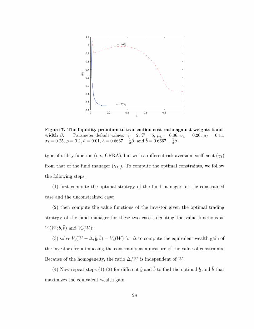
In Figure 7, we plot the liquidity premium to transaction cost ratio δ/α against the
constraint stringency β. This figure shows that when the constraint is very stringent,
the ratio can be much greater than what Constantinides (1986) finds (where it is
typically around 0.1). Thus in contrast to Constantinides (1986), transaction costs
can have a first-order effect in the presence of stringent portfolio constraints. This is
because imposing stringent constraints can force more frequent transactions and also
can significantly distort the investment strategy. This figure also shows that for a
26

given constraint bandwidth β, the liquidity premium is much higher if the volatility
of the illiquid stock is high. For example, the ratio becomes as high as 0.95 when
σI = 0.4 and β = 0.2. Surprisingly, the dashed line shows that the liquidity premium
can increase when the constraints become less stringent (i.e, as β increases). The main
reason for this counterintuitive result is the presence of binding constraints. When
σI = 0.4, the Merton line for this case is 0.2917. The lower bound at β = 0.02, for
example, is b = 0.6427 and thus binding in the no transaction cost case. This implies
that the value function shifts upward in both the case with transaction costs and the
case without transaction costs as β increases. More importantly, as β increases from
0.02 and thus b decreases, the investment in the illiquid asset decreases. It follows that
it takes a larger reduction in the expected return µI to decrease the value function
J by the same amount. It is this effect that makes the liquidity premium go up in
this region when the constraints become less binding. Figure 7 also shows that as the
constraint becomes more relaxed, the liquidity premium starts to decline again. To
understand this eventual decreasing pattern, it is helpful to consider the extreme case
where the constraints do not bind for the no transaction cost case. Therefore, as the
constraints become more relaxed, the value function with transaction costs increases
and thus the liquidity premium decreases until the constraints become non-binding
even for the case with transaction costs, then the liquidity premium stays constant.
Now we briefly examine the issue of the optimal choice of the constraints by in-
vestors who hire fund managers. There are many possible reasons why investors
might constrain their managers, e.g., different preferences, different investment hori-
zons, asymmetric information, moral hazard, etc. In the subsequent analysis, for
illustration purposes, we focus on the case where the only difference between in-
vestors and managers is risk aversion. Specifically, suppose the investor has the same
27
0 0.2 0.4 0.6 0.8 10.2
0.3
0.4
0.5
0.6
0.7
0.8
0.9
1
1.1
β
δ/α
σ =40%
σ =25%
Figure 7. The liquidity premium to transaction cost ratio against weights band-width β. Parameter default values: γ = 2, T = 5, µL = 0.06, σL = 0.20, µI = 0.11,σI = 0.25, ρ = 0.2, θ = 0.01, b = 0.6667− 1
2β, and b = 0.6667 + 12β.
type of utility function (i.e., CRRA), but with a different risk aversion coefficient (γI)
from that of the fund manager (γM). To compute the optimal constraints, we follow
the following steps:
(1) first compute the optimal strategy of the fund manager for the constrained
case and the unconstrained case;
(2) then compute the value functions of the investor given the optimal trading
strategy of the fund manager for these two cases, denoting the value functions as
Vc(W ; b, b) and Vu(W );
(3) solve Vc(W −∆; b, b) = Vu(W ) for ∆ to compute the equivalent wealth gain of
the investors from imposing the constraints as a measure of the value of constraints.
Because of the homogeneity, the ratio ∆/W is independent of W .
(4) Now repeat steps (1)-(3) for different b and b to find the optimal b and b that
maximizes the equivalent wealth gain.
28

We illustrate the optimal choice through two cases: One case where the investor
is less risk averse than the manager (Figure 8) and the other case where the investor
is more risk averse (Figure 9). Specifically, we set γI = 2 and γM = 5 in Figure 8
and γI = 5 and γM = 2 in Figure 9. This implies that in Figure 8 (Figure 9) the
investor would like the manager to invest more (less) in the illiquid stock than what
the manager would choose to. So we only consider the imposition of a lower (upper)
bound in Figure 8 (Figure 9). Figure 8 plots the ratio ∆/W against b and Figure
9 plots the ratio ∆/W against b for different correlation coefficients and transaction
cost rates, where the stars in the figures indicate where the ratios are maximized.
Figure 8 shows that the optimal lower bound b is equal to 0.624 in the first case
(given default parameter values) and Figure 9 shows that the optimal upper bound
b is equal to 0.520 in the second case . These figures also show that as transaction
cost rate increases, the optimal choice of the lower bound decreases and the optimal
upper bound increases. Intuitively, as transaction cost rate increases, the illiquid
stock becomes more costly to trade and thus the investor imposes looser constraints.
Interestingly, these figures also suggest that as the correlation increases while the
optimal upper bound decreases, the optimal lower bound increases. This is driving by
the fact that how the correlation coefficient affects the trading strategy depends on
the magnitude of the risk aversion. If the risk aversion is high, then as the correlation
increases, the investor decreases the investment in the illiquid asset to reduce the
risk. As correlation increases, portfolio risk increases because diversification is less
effective. To counter this adverse effect, an investor can either increase its illiquid
asset to achieve a higher expected return or reduce it to decrease risk. If the risk
aversion is low, then it is optimal for the investor to increase the investment in the
illiquid asset. If the risk aversion is high, then it is optimal for the investor to decrease
29

0.3 0.4 0.5 0.6 0.7 0.8 0.90
0.005
0.01
0.015
0.02
0.025
0.03
b
∆/W =0.5ρ
=0.6ρ
α=5%
_
Figure 8. The optimal choice of the lower bound for an investor. Parameterdefault values: γI = 2, γM = 5, T = 5, µL = 0.06, σL = 0.20, µI = 0.11, σI = 0.25, ρ = 0.2,α = 0.01, θ = 0.01, and b = 0.80.
it. In Figure 8, the investor’s risk aversion is low, so as the correlation increases, the
optimal level of illiquid asset investment becomes higher, and thus he imposes a higher
lower bound. In Figure 9, the investor’s risk aversion is high, so as the correlation
increases, the optimal level of illiquid asset investment becomes lower, and thus he
imposes a lower upper bound.
These figures also demonstrate that the benefit of constraining fund managers can
be quite significant. Figure 8 suggest that the investor is willing to pay more than
0.86% of the initial wealth for the right to constrain fund managers. In Figure 9, the
gain from imposing portfolio constraints is as high as 2.71%. The right to impose
constraints becomes even greater the correlation is high (e.g., 5.4% when ρ = 0.6 in
Figure 9).
30

0.3 0.4 0.5 0.6 0.7 0.8 0.90
0.01
0.02
0.03
0.04
0.05
0.06
/W∆
α=5%
ρ=0.6
=0.5ρ
b_
Figure 9. The optimal choice of the upper bound for an investor. Parameterdefault values: γI = 5, γM = 2, T = 5, µL = 0.06, σL = 0.20, µI = 0.11, σI = 0.25, ρ = 0.2,α = 0.01, θ = 0.01, and b = 0.
VI. Conclusions
We use a novel approach to examine the optimal investment problem of a mutual fund
who faces transaction costs and portfolio constraints. We show that both the buy
boundary and the sell boundary for the illiquid stock are monotonically decreasing in
the portfolio bounds.
We find that the presence of portfolio constraints can significantly magnify the
effect of transaction costs on liquidity premium and can make it a first-order effect
for a reasonable set of parameter values. Surprisingly, the liquidity premium can
increase when binding constraints become less stringent. We also show that even
for log preferences, the optimal trading strategy is nonmyopic with respect to the
constraints, in the sense that currently nonbinding constraints can affect the current
optimal trading strategy. In addition, the optimal buy boundary is monotonically
31

decreasing in calendar time. We also examine the endogenous choice of the portfolio
bounds. Our analysis shows that the optimal upper is increasing in transaction costs
and the optimal lower bound is decreasing in transaction costs.
32

A APPENDIX
In this Appendix, we present proofs for the propositions and theorems in this paper.
A.1 Proof of Theorem 1
Given πIs , we denote
σ(s) =
√1
2
[(1− πIs)
2σ2L + 2ρ(1− πIs)πIsσLσI + π2
Isσ2
I
].
Then
WT = WteR T
t [(1−πIs)µL+πIsµI−σ2(s)ds+R T
t (1−πIs)σLdBLs+R T
t πIsσIdBIs .
Therefore
EW 1−γT
= W 1−γt E[e(1−γ)
R Tt [(1−πIs)µL+πIsµI−σ2(s)]ds+
R Tt (1−γ)(1−πIs )σLdBLs+
R Tt (1−γ)πIsσIdBIs ]
= W 1−γt E[e(1−γ)
R Tt [(1−πIs )µL+πIsµI−γσ2(s)]dsZ(T )]
≡ W 1−γt E[e(1−γ)
R Tt f(πIs )dsZ(T )],
where Z(ν) = e−R ν
t (1−γ)2σ2(s)ds+R ν
t (1−γ)(1−πIs )σLdBLs+R ν
t (1−γ)πIsσIdBIs is a nonnegative
local martingale, therefore supermartingale with E[Z(T )] ≤ Z(t) = 1, and
f(ξ) = (1− ξ)µL + ξµI − γ
2[(1− ξ)2σ2
L + 2ρ(1− ξ)ξσLσI + ξ2σ2I ].
Denote η = maxx∈IR,ξ∈[b,b] f(ξ), and denote the maximizer as ξ∗. It is easy to see
ξ∗ = π∗I , η = f(π∗I ).
We then deduce
EW 1−γT ≤ W 1−γ
t e(1−γ)η(T−t)E[Z(T )]
≤ (Wteη(T−t))(1−γ),
and the equality holds if and only if πIs ≡ π∗I .
33

A.2 Proof of Proposition 1
We only prove part 1, and the case of part 2 is similar. Let
w =1
1− γlog [(1− γ) ϕ] .
It is not hard to see that w(π, t) satisfies
max
wt + L2w,− α
1−απ− wπ, wπ − θ
1+θπ
= 0
w(π, T ) = 0, in(−1
θ, 1
α
)× [0, T ),
where
L2w =1
2β1π
2 (1− π)2 [wππ + (1− γ) w2
π
]+ β2π (1− π) wπ + β3 + β2π − 1
2γβ1π
2.
Denote
v(π, t) = wπ(π, t).
Clearly
∂
∂π(L2w)
=1
2β1π
2 (1− π)2 vππ + [β1 + β2 − (2 + γ) β1π] π (1− π) vπ
+ [β2 (1− 2π)− γβ1π(2− 3π)] v
+ (1− γ) β1π (1− π) v [(1− 2π) v + π (1− π) vπ] + β2 − γβ1π
∆= Lv.
Using the same technique as in Dai and Yi (2006), we are able to show that v(π, t)
satisfies the following parabolic double obstacle problems:
vt + Lv = 0 if − α1−απ
< v < θ1+θπ
,
vt + Lv ≤ 0 if v = − α1−απ
,
vt + Lv ≥ 0 if v = θ1+θπ
,
v(π, T ) = 0,
(A-1)
in(−1
θ, 1
α
)× [0, T ).
34

It is not hard to verify
0 ≥(
∂
∂t+ L
)(− α
1− απ
)=
1− α
(1− απ)3 [β2 − (γβ1 − αγβ1 + αβ2) π]
=(1− α) γβ1
(1− απ)3
[πM
I − (1− α + απM
I
)π].
Since 1− α + απMI > 0, it follows
πI(t) ≥ πMI
1− α (1− πMI )
.
It remains to show that there exists t < T such that πI(s) = 1α
for s ∈ (t, T ).
Suppose not, we then infer v(π, t) is smooth across π = πI(t), t < T. It follows
π′I(t)vπ + vt|π=πI(t) =d
dtv (πI(t), t) =
d
dt
(− α
1− απI(t)
)
= − α2π′I(t)
(1− απI(t))2 = π′I(t)vπ|π=πI(t) , for t < T,
which yields
vt|π=πI(t) = 0, for t < T.
On the other hand, v(π, t) clearly has a singularity at(
1α, T
), i.e.
limπ→ 1
α, t→T
vt (π, t) = +∞.
A contradiction.
A.3 Proof of Proposition 2
Note that the differential operator L is degenerate at π = 0, 1, which yields two
ordinary differential inequalities there:
vt(0, t) + β2v(0, t) + β2 = 0 if − α < v(0, t) < θvt(0, t) + β2v(0, t) + β2 ≤ 0 if v(0, t) = −αvt(0, t) + β2v(0, t) + β2 ≥ 0 if v(0, t) = θv(0, T ) = 0.
35

and
vt(1, t)− β4v(1, t) + β4 = 0 if − α1−α
< v(1, t) < θ1+θ
vt(1, t)− β4v(1, t) + β4 ≤ 0 if v(1, t) = − α1−α
vt(1, t)− β4v(1, t) + β4 ≥ 0 if v(1, t) = θ1+θ
v(1, T ) = 0.
Solving them, we then obtain
v(0, t) =
eβ2(T−t) − 1, when t > t0−α, when t ≤ t0
if β2 < 0 (A-2)
v(0, t) =
eβ2(T−t) − 1, when t > t0θ, when t ≤ t0
if β2 > 0 (A-3)
v(0, t) = 0 if β2 = 0 (A-4)
and
v(1, t) =
1− e−β4(T−t), when t > t1− α
1−α, when t ≤ t1
if β4 < 0 (A-5)
v(1, t) =
1− e−β4(T−t), when t > t1
θ1+θ
, when t ≤ t1if β4 > 0 (A-6)
v(1, t) = 0 if β4 = 0. (A-7)
Now let us prove part 1. If πMI < 0, then β2 < 0 and β4 < 0. So, we have (A-2) and
(A-5), which implies that πI(t) < 0 for all t, and πI(t) intersects with the lines π = 0
and π = 1 at t0 and t1 respectively. We then infer πI(t) ≤ 0 for t < t0, 0 ≤ πI(t) ≤ 1
for t ∈ [t0, t1
], and πI(t) ≥ 1 for t > t1.
To show the monotonicity of πI(t) for t > t0, let us introduce the comparison
principle that plays a critical role in the subsequent proofs.
Comparison principle for double obstacle problem (cf. Friedman (1982))
Let vi, i = 1, 2, satisfy
∂vi
∂t+ Lvi + fi = 0, if gl
i < vi < gui ,
∂vi
∂t+ Lvi + fi ≤ 0, if vi = gl
i,
∂vi
∂t+ Lvi + fi ≥ 0, if vi = gu
i ,
36

in Ω× [0, T ). Here L is an elliptic operator. Assume
f1 ≤ f2; gl1 ≤ gl
2; gu1 ≤ gu
2 in Ω× [0, T )
and
v1 ≤ v2 on t = T and ∂Ω× [0, T ).
Then
v1 ≤ v2 in Ω× [0, T ).
Note that
vt|t=T = −Lv|t=T = −β2 + γβ1π ≥ 0 for π > 0.
Applying the comparison principle gives vt ≥ 0 in π > 0, which yields the desired
result.
The proof of part 2-4 is similar for finite T . In part 4, if T = ∞, we then follow
Dai and Yi (2006) to take into account the corresponding stationary problem, from
which we can infer πI(t) = πI(t) = 0 when πMI = 0 and πI(t) = πI(t) = 1 when
πMI = 1.
A.4 Proof of Theorem 2
The uniqueness of viscosity solution can be obtained by using a similar argument
in Akian, Mendaldi and Sulem (1996) (see also Crandal, Ishii and Lions (1992)).
Here we highlight that on the boundaries the solution is a viscosity supersolution. In
terms of the definition of viscosity solution and the Ito’s formula for a C2 function
of a stochastic process with jump, we are able to show that the value function is a
viscosity solution to the HJB equation (see, for example, Shreve and Soner (1994)).
Part ii) can be obtained using the same technique as in Dai and Yi (2006).
37
A.5 Proof of Proposition 4
1. For the constrained case, we can similarly obtain the following double obstacle
problem:
vt + Lv = 0 if − α1−απ
< v < θ1+θπ
,
vt + Lv ≤ 0 if v = − α1−απ
,
vt + Lv ≥ 0 if v = θ1+θπ
,
v(z, T ) = 0,
(A-8)
subject to boundary conditions
v (b, t) = θ
1+θπ,
v(b, t
)= − α
1−απ,
(A-9)
in(b, b
) × [0, T ). Denote the solution of the above problem by v(π, t; b, b). Assume
b1 ≥ b2. Since
v(b2, t; b, b1) ≤ θ
1 + θb= v(b2, t; b, b2),
we get by the comparison principle
v(π, t; b, b1) ≤ v(π, t; b, b2) in(max (b, 0) , b2
)× [0, T ).
So, if v(π, t; b, b2) < θ1+θπ
, then
v(π, t; b, b1) <θ
1 + θπ,
which implies πcI(t; b, b1) ≥ πc
I(t; b, b2), namely, πcI(t; b, b) is increasing with b. In a
similar way, we can show that πcI(t; b, b) is increasing with b and πc
I(t; b, b) is increasing
with b and b.
2 and 3. We will only prove one case b > 0, and the other cases are similar. As in
the proof of Proposition 2, we can still derive the boundary conditions (A-2)-(A-4) at
π = 0. So, we can deal with the problem in π ≤ 0 and 0 ≤ π ≤ b independently.
This yields the desired result.
38

A.6 Proof of Propositions 5 and 6
Still, we use the fact that the problem can be dealt with in π ≤ 0, 0 ≥ π ≤ 1 and
π ≥ 1 independently. The remaining argument is similar to the proof of Proposition
2.
39

References
Akian, Marianne, Jose Luis Menaldi, and Agnes Sulem, 1996, “On an investment-
consumption model with transaction costs,” SIAM Journal on Control and Optimiza-
tion 34, 329–394.
Almazan, Andres, Keith C. Brown, Murray Carlson, and David A. Chapman, 2004,
“Why constrain your mutual fund manager?” Journal of Financial Economics 73,
289-321.
Basak, S., A. Pavlova, and A. Shapiro, 2006, “Optimal asset allocation and risk
shifting in money management,” forthcoming, Review of Financial Studies.
Carpenter, J., 2000, Does option compensation increase managerial risk appetite,
Journal of Finance 55, 2311–2331.
Chalmers, John M. R. , Roger M. Edelen, and Gregory B. Kadlec, “An analysis of
mutual fund trading costs,” working paper, University of Pennsylvania.
Chevalier, Judith, and Glen Ellison, 1997, “Risk taking by mutual funds as a response
to incentives,” Journal of Political Economy 105, 1167-1200.
Clarke, Roger, Harindra de Silva, and Steven Thorley, 2002. “Portfolio constraints
and the fundamental law of active management,” Financial Analysts Journal 58,
48-66.
Constantinides, George M., 1986, “Capital market equilibrium with transaction costs,”
The Journal of Political Economy 94, 842–862.
Cuoco, Domenico, 1997, “Optimal consumption and equilibrium prices with portfolio
constraints and stochastic income,” Journal of Economic Theory 72, 33–73.
40

Cuoco, Domenico and Hong Liu, 2000, “A martingale characterization of consumption
choices and hedging costs with margin requirements, ” Mathematical Finance 10, 355–
385.
Cvitanic, Jasak and Ioannis Karatzas, 1992, “Convex duality in constrained portfolio
optimization,” Annals of applied probability 2, 767–818.
Dai, Min, and Fahuai Yi, 2006, “Finite horizon optimal investment with transaction
costs: a parabolic double obstacle problems,” working paper, National University of
Singapore.
Dai, Min, Lishang Jiang and Fahuai Yi, 2006, “A parabolic variational inequality with
gradient constraint arising from optimal investment and consumption with transac-
tion costs,” working paper, National University of Singapore.
Dai, Min, Yue Kuen Kwok and Jianping Zong, 2007, Guaranteed minimum with-
drawal benefit in variable annuities, forthcoming, Mathematical Finance.
Davis, Mark H.A., and Andrew R. Norman, 1990, “Portfolio selection with transaction
costs,” Mathematics of Operations Research 15, 676–713.
Delib, Daniel N., and Raj Varma, 2002, “Contracting in the investment management
industry: evidence from mutual funds,” Journal of Financial Economics 63, 79–98.
Fleming, Wendell H. and H. Mete Soner, 1993, Controlled Markov Processes and
Viscosity Solutions, New York, Springer.
Forsyth, Peter A. and K. R. Vetzal, 2002, “Quadratic convergence of a penalty method
for valuing American options,” SIAM Journal of Scientific Computations 23, 2095–
2122.
41

Friedman, Avner, 1982, Variational principles and free-boundary problems, Wiley,
New York.
Huang, Lixin and Hong Liu, 2007, “Rational inattention and portfolio selection,”
forthcoming, Journal of Finance.
Liu, Hong, 2004, “Optimal consumption and investment with transaction costs and
multiple risky assets,” Journal of Finance 59, 289–338.
Liu, Hong, and Mark Loewenstein, 2002, “Optimal portfolio selection with transaction
costs and finite horizons,” The Review of Financial Studies 15, 805–835.
Merton, Robert C., 1971, “Optimum consumption and portfolio rules in a continuous-
time model,” Journal of Economic Theory 3, 373–413.
Michael G. Crandall, Hitoshi Ishii, and Pierre-Louis Lions, 1992, “User’s guide to
viscosity solutions of second order partial differential equations,” Bulletin of The
American Mathematical Society 27, 1–67.
Royden, Halsey L., 1988, Real Analysis, Macmillan, New York.
Shreve, Steven E., and H. Mete Soner, 1994, “Optimal investment and consumption
with transaction costs,” The Annals of Applied Probability 4, 609–692.
42


