
IMPLEMENTATION OF FILTERING BEAMFORMING ALGORITHMS FOR SONAR DEVICES USING GPU
by
Shahrokh Kamali
Submitted in partial fulfilment of the requirements for the degree of Master of Applied Science
at
Dalhousie University Halifax, Nova Scotia
June 2013
© Copyright by Shahrokh Kamali, 2013

ii
DEDICATION PAGE
To my wife Sussan and my son Arash for their love and encouragement.
iii
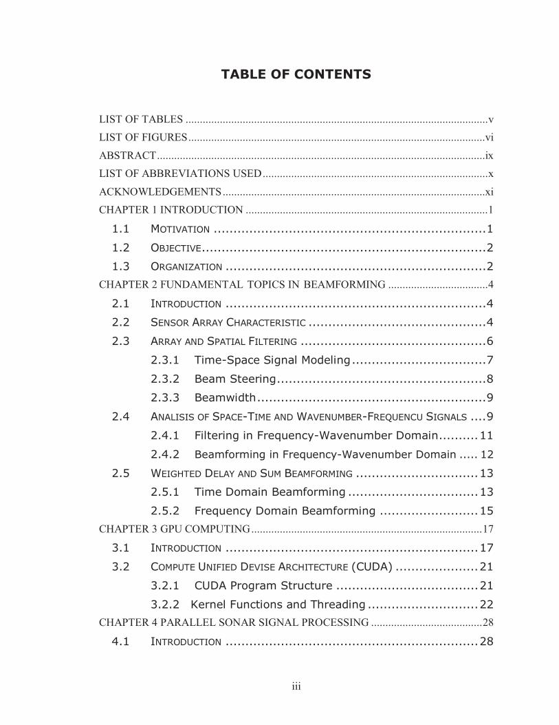
TABLE OF CONTENTS
LIST OF TABLES .......................................................................................................... v LIST OF FIGURES ........................................................................................................vi
ABSTRACT ...................................................................................................................ix LIST OF ABBREVIATIONS USED ............................................................................... x
ACKNOWLEDGEMENTS ............................................................................................xi CHAPTER 1 INTRODUCTION ..................................................................................... 1
1.1 MOTIVATION ..................................................................... 1
1.2 OBJECTIVE ........................................................................ 2
1.3 ORGANIZATION .................................................................. 2 CHAPTER 2 FUNDAMENTAL TOPICS IN BEAMFORMING ................................... 4
2.1 INTRODUCTION .................................................................. 4
2.2 SENSOR ARRAY CHARACTERISTIC ............................................. 4
2.3 ARRAY AND SPATIAL FILTERING ............................................... 6
2.3.1 Time-Space Signal Modeling .................................. 7
2.3.2 Beam Steering ..................................................... 8
2.3.3 Beamwidth .......................................................... 9
2.4 ANALISIS OF SPACE-TIME AND WAVENUMBER-FREQUENCU SIGNALS .... 9
2.4.1 Filtering in Frequency-Wavenumber Domain .......... 11
2.4.2 Beamforming in Frequency-Wavenumber Domain ..... 12
2.5 WEIGHTED DELAY AND SUM BEAMFORMING ............................... 13
2.5.1 Time Domain Beamforming ................................. 13
2.5.2 Frequency Domain Beamforming ......................... 15 CHAPTER 3 GPU COMPUTING ................................................................................. 17
3.1 INTRODUCTION ................................................................ 17
3.2 COMPUTE UNIFIED DEVISE ARCHITECTURE (CUDA) ..................... 21
3.2.1 CUDA Program Structure .................................... 21
3.2.2 Kernel Functions and Threading ............................ 22 CHAPTER 4 PARALLEL SONAR SIGNAL PROCESSING ....................................... 28
4.1 INTRODUCTION ................................................................ 28

iv
4.2 PREPARING DATA AND PARAMETERS ........................................ 30
4.3 ZERO PADDING ................................................................ 32
4.4 2D FFT ON TIME-SPACE DOMAIN........................................... 34
4.5 SPATIAL FILTERING (K- MASKING) ........................................ 35
4.6 TIME DELAY MASKING ........................................................ 39
4.7 SUMMATION .................................................................... 40 CHAPTER 5 RESULTS ................................................................................................ 42
5.1 BEAMFORMING BY CPU SEQUENTIAL AND GPU COMPUTATION .......... 42
5.1.1 Using GPU As A Beamformer .............................. 43
5.1.2 Real-Time Beamformer ...................................... 43
5.1.3 Accuracy .......................................................... 43 CHAPTER 6 CONCLUSION ........................................................................................ 45
6.1 CPU SEQUENTIAL AND GPU COMPUTATION COMPARISON ............... 45 BIBLIOGRAPHY ......................................................................................................... 54

v
LIST OF TABLES
Table 5.1 Time usage comparison between MATLAB code and CUDA code .............. 42 Table 6.1 CPU sequential and GPU computation usage times ...................................... 46 Table 6.2 Speed comparison between CPU sequential and GPU computation .............. 47

vi
LIST OF FIGURES Figure 2.1 Deployment of acoustic sensor array in an ocean.………………..………..5 Figure 2.2 A three dimensional coordinate system.…………………………..……….6
Figure 2.3 Projection of a plane wave on the linear array.……….…………..……….7 Figure 2.4 (k, ) space corresponding………………………….………………........10 Figure 2.5 Passband of an ideal beamformer l……………………………………….12 Figure 2.6 Time domain beamformer..………………………………………..……..14 Figure 2.7 Frequency domain beamformer..…………………...……………….……16
Figure 3.1 Enlarging Performance Gap between GPUs and CPUs..…………….......19 Figure 3.2 Fundamentally different design philosophies between CPU and GPU.....19
Figure 3.3 GeForce GTX 690 GPU card from NVIDIA…………………………....20 Figure 3.4 The element by element matrix multiplication kernel function……..........23 Figure 3.5 CUDA thread organization...…...………………………………………..24 Figure 3.6 Simple program to add two long vectors element by element.…...….…..26 Figure 4.1 Main algorithm for digital beamforming by GPU computing.……....…..29 Figure 4.2 Geometry of a linear array of equally spaced sensors.……...…………...30
Figure 4.3 Data matrix y in Space-Time (x-t) domain.……………………...............31 Figure 4.4 Sample data as an input for one sensor.………………………….………31
Figure 4.5 Sample data as an input on 64 sensors.…………………………….…….32 Figure 4.6 Data matrix y in Space-Time (x-t) domain.……………………..….……33
Figure 4.7 Raw signal in k- domain.………………………………………………34 Figure 4.8 23 Array beams uniformly distribution on sin ( ).……………...……...35
Figure 4.9 k – Filter Mask for beam angle = 46.6582o.…………………………..36

vii
Figure 4.10 Filtered signal in Space – Time domain for beam angle = 46.6582o….....37
Figure 4.11 Filtered signal in k- domain for beam angle = 46.6582o.……………. 37 Figure 4.12 Raw data & filtered data on one sensor for steering beam = 46.6582o…..38
Figure 4.13 Summation procedure for each steering angle…………………………….40 Figure 4.14 Filtered and time delayed signal in k- domain...………….…………….41
Figure 4.15 Raw data on one sensor and beamformer output.……….………………...41 Figure 6.1 Usage time to execute just on kernel on GPU…………….…………...…45 Figure 6.2 2D FFT CPU sequential and GPU computation usage time comparison…..…………………………………………………………...48 Figure 6.3 2D FFT speed comparison between CPU sequential and GPU
computation.……………………………………………………………...48 Figure 6.4 2D IFFT CPU sequential and GPU computation usage time comparison.………………………………………………………………49 Figure 6.5 2D IFFT speed comparison between CPU sequential and GPU
computation.……………………………………………………………...49 Figure 6.6 1D FFT CPU sequential and GPU computation usage time comparison.………………………………………………………………50 Figure 6.7 1D FFT speed comparison between CPU sequential and GPU
computation.……………………………………………………………...50 Figure 6.8 1D IFFT CPU sequential and GPU computation usage time comparison.………………………………………………………………51 Figure 6.9 1D IFFT speed comparison between CPU sequential and GPU
computation.……………………………………………………………...51 Figure 6.10 Zero Padding CPU sequential and GPU computation usage time comparison.………………………………………………………………52 Figure 6.11 Zero Padding speed comparison between CPU sequential and GPU
computation.……………………………………………………………...52 Figure 6.12 Summation CPU sequential and GPU computation usage time comparison.………………………………………………………………53

viii
Figure 6.13 Summation speed comparison between CPU sequential and GPU
computation.……………………………………………………………...53

ix
ABSTRACT Beamforming is a signal processing technique used in sensor arrays to direct signal
transmission or reception. Beamformer combines input signals in the array to achieve
constructive interference at particular angles (beams) and destructive interference for
other angles.
According to the following facts:
1- Beamforming can be computationally intensive, so real-time sonar beamforming
algorithms in sonar devices is important.
2- Parallel computing has become a critical component of computing technology of
the 1990s, and it is likely to have as much impact over the next 20 years as
microprocessors have had over the past 20 [5].
3- The high-performance computing community has been developing parallel
programs for decades. These programs run on large scale, expensive computers.
Only a few elite applications can justify the use of these expensive computers [2].
4- GPU computing has the ability of parallel computing and it could be available on
the personal computers.
The objective of this thesis is to use Graphics Processing Unit (GPU) as real-time digital
beamformer to accelerate the intensive signal processing.

x
LIST OF ABBREVIATIONS USED
ALU Arithmetic Logic Unit CPU Central Processing Unit CUDA Computer Unified Device Architecture DFT Discrete Fourier Transform DRAM Dynamic Random Access Memory FFT Fast Fourier Transform GFLOPS Giga FLoating-point Operations Per Second GPU Graphics Processing Unit IFFT Inverse Fast Fourier Transform MACs multiply accumulates SNR Signal to Noise Ratio SPMD Single-Program Multiple-Data

xi
ACKNOWLEDGEMENTS
It is with immense gratitude that I acknowledge the support and help of my supervisor Dr. Joshua Leon. I have learned a lot from his unrivalled knowledge in parallel programming architecture and algorithms, digital signal processing and GPU computation. Dr. Leon has shed lights on the problems as a mentor. I wish other students have opportunity to learn from his wisdom. I want to thank Dr. Olivier Beslin. I am impressed by his knowledge and experience in Beamforming and I owe him my understanding of Sonar Beamforming. I would like to express my appreciation to all faculties of Electrical and Computer Engineering specially Dr. Michael Cada, Dr. Jason Gu and Dr. Geoff Maksym faculty of Biomedical Engineering for whatever I learned at Dalhousie University. I am grateful to Engineering Dean’s office staff and Electrical and Computer Engineering office staff.
1
CHAPTER 1 INTRODUCTION
1.1 MOTIVATION
Beamforming has many applications in radar, sonar, seismology, wireless
communications, radio astronomy, acoustics, and biomedicine. Beamforming is used to
detect a signal of interest coming from specific direction. A beamformer algorithm
process sensor array signals in order to increase Signal to Noise Ratio (SNR). It
manipulates large complex matrices and involves a large number of Fast Fourier
Transforms (FFT) in order to perform a multi-dimensional filtering in space-time or
wavenumber-frequency domains.
Expensive custom hardware and software is required to process data intensive sonar
beamforming algorithm in real-time. Real-time signal processing in sonar devices is very
important. High-resolution sonar consists of an array of underwater sensors and a
beamformer to determine from which direction the signal is coming. The sensor element
outputs are filtered and combined to construct a set of beams, each beam pointing in a
specific direction.
To accelerate the signal processing speed we implemented parallel processing technique
by using the Graphics Processing Unit (GPU) as a real-time digital beamformer.
INVIDIA GeForce 690 with 4GB RAM GPU and CUDA programming language have
been used to speed up beamforming algorithms. CUDA is a parallel computing platform
and programming model invented by NVIDIA. It enables dramatic increases in
computing performance by harnessing the power of the GPU.
GPU computing or GPGPU is the use of GPU as a co-processor to speed up scientific and
engineering computing. The GPU accelerates applications running on the CPU by
removing some of the compute intensive and time consuming portions of the code and
executing them separately on GPU in parallel or sequential form. However, part of the
applications run sequentially on the CPU. The application runs faster as it is using the
power of the GPU to process parallel processing part of the algorithm and boost
performance. This is known as “heterogeneous” or “hybrid” computing.
2
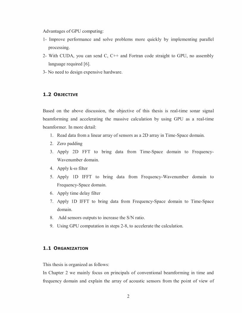
Advantages of GPU computing:
1- Improve performance and solve problems more quickly by implementing parallel
processing.
2- With CUDA, you can send C, C++ and Fortran code straight to GPU, no assembly
language required [6].
3- No need to design expensive hardware.
1.2 OBJECTIVE
Based on the above discussion, the objective of this thesis is real-time sonar signal
beamforming and accelerating the massive calculation by using GPU as a real-time
beamformer. In more detail:
1. Read data from a linear array of sensors as a 2D array in Time-Space domain.
2. Zero padding
3. Apply 2D FFT to bring data from Time-Space domain to Frequency-
Wavenumber domain.
4. Apply k- filter
5. Apply 1D IFFT to bring data from Frequency-Wavenumber domain to
Frequency-Space domain.
6. Apply time delay filter
7. Apply 1D IFFT to bring data from Frequency-Space domain to Time-Space
domain.
8. Add sensors outputs to increase the S/N ratio.
9. Using GPU computation in steps 2-8, to accelerate the calculation.
1.1 ORGANIZATION
This thesis is organized as follows:
In Chapter 2 we mainly focus on principals of conventional beamforming in time and
frequency domain and explain the array of acoustic sensors from the point of view of

3
performing spatial filtering. In Chapter 3 the general idea of GPU computation is
discussed. CUDA programming, kernel and threads, three important GPU computation
subjects, are also explained. Chapter 4 describes our approach to do beamforming by
using GPU computation and explained our beamforming algorithm. Chapter 5 compares
the speed and accuracy of implementation of filtering beamforming algorithm for sonar
devices using GPU with already exist sequential beamforming algorithm.

4
CHAPTER 2 FUNDAMENTAL TOPICS IN BEAMFORMING
2.1 INTRODUCTION
In this chapter we introduce the fundamentals of beamforming. Beamforming is the art of
manipulating array sensor data to extract a signal of interest from noise when looking in a
specific direction. All directions are explored simultaneously through a set of beams.
Beamforming can be interpreted as a bandpass filter in space and time.
The principal focus of this chapter is the digital processing of signals received by a linear
array of spatially distributed sensors. One part of the processing of signals is to separate a
signal from noise, interference and other undesirable signals.
Beamforming systems are designed to detect incoming signals that have interference with
other signals. Sometimes the desired signal and interferers have the same frequency band,
then frequency filtering is not useful to separate desired signal from interference.
However, if the desired signals and interfering signals come from different spatial
locations, then the spatial separation can be used to separate signal from interference by
applying a spatial filter [19].
Beamforming algorithm deals with the localization of signals in time domain, frequency
domain, direction of propagation, or some other variable, so the signals are
multidimensional and multidimensional digital filtering is useful to solve the problem of
extracting information from a signals received by linear array sensors. This algorithm
provides a processing system to separate signals with a particular set of parameters value
from other signals.
2.2 SENSOR ARRAY CHARACTERISTIC
Towed array sonar is a sonar array that is towed behind a submarine or surface ship. It
includes a cable and some hydrophones (sensors). The hydrophones are placed at specific
distances along the cable. (Figure 2.1)

5
Figure 2.1: Deployment of acoustic sensor array in an ocean
Active sonar transmits acoustic energy into the water and processes received echoes. The
active sonar has a lot of common subjects with radars. However, the important difference
between sonar and radar is that the propagation of acoustic energy in the ocean is more
complicated than the propagation of electromagnetic energy in the air. The complication
factors of acoustic energy propagation must be considered in the design of sonar systems.
These factors include spreading loss, absorption, and ducting. These factors will change
and depend on the other factors such as desired range of sonar, the depth of the water,
and the nature of the boundaries.
Passive sonar systems receive the incoming acoustic energy and process it to observe the
characteristics of incoming signals. The most important application of passive sonar is
the detection and tracking of submarines. All complication factors of acoustic energy
propagation and noise also apply to the passive sonar case [8].
The advantages of a sensor line array (versus a signal hydrophone) include reduced
response to the noise emanating from the platform and by using long arrays, relatively
better performance at low frequency. The length of array has direct relation with
frequency, which means, longer the array, the lower is the frequency range for which
acceptable performance can be achieved.
A disadvantage of sensor line array is that a source can be recognized only relative to a
conic angle. In other words, without additional information, it is not possible to generate
azimuth and elevation components from this conic angle. It means that without additional
6
information, we cannot specify on which side of array the source is located. We have to
consider the fact that the linear array of sensors is never exactly horizontal or straight and
it will cause some uncertainties in sensor positions, which degrade the beamforming
calculation [7].
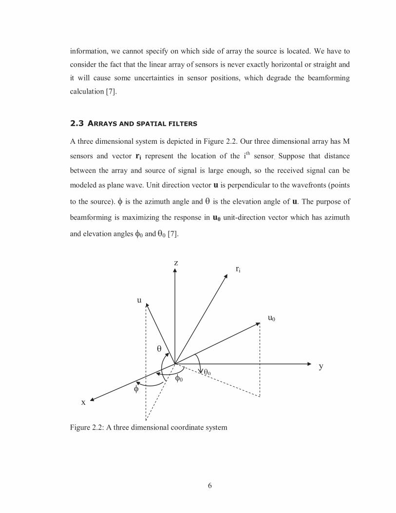
2.3 ARRAYS AND SPATIAL FILTERS
A three dimensional system is depicted in Figure 2.2. Our three dimensional array has M
sensors and vector ri represent the location of the ith sensor. Suppose that distance
between the array and source of signal is large enough, so the received signal can be
modeled as plane wave. Unit direction vector u is perpendicular to the wavefronts (points
to the source). is the azimuth angle and is the elevation angle of u. The purpose of
beamforming is maximizing the response in u0 unit-direction vector which has azimuth
and elevation angles and [7].
Figure 2.2: A three dimensional coordinate system
u
ri
u0
z
y
x
7
2.3.1 Time-Space signal Modeling Suppose a complex sinusoid signal with unit-direction vector u, is propagating through
the water, so the received signal at the ith sensor is:
xi(n) = exp[j(2 fn/fs + kri.u)], i= 1, 2, …, M (2.1)
k=2 f/c is the wavenumber
fs is the sampling frequency
f is the frequency and is equal to c/
c is the speed of sound in the medium and is the wave length
If we add all received signal at the M sensors in the array:
y(n) = xi(n) = exp(j2 fn/fs) exp(jkri.u) (2.2)
Where the factor:
b(f, u exp(jkri.u)
Is complex beam pattern. The dot product in (2.2) and (2.1) is equal to:
ri.u = rxicos cos + ryisin cos + rzisin
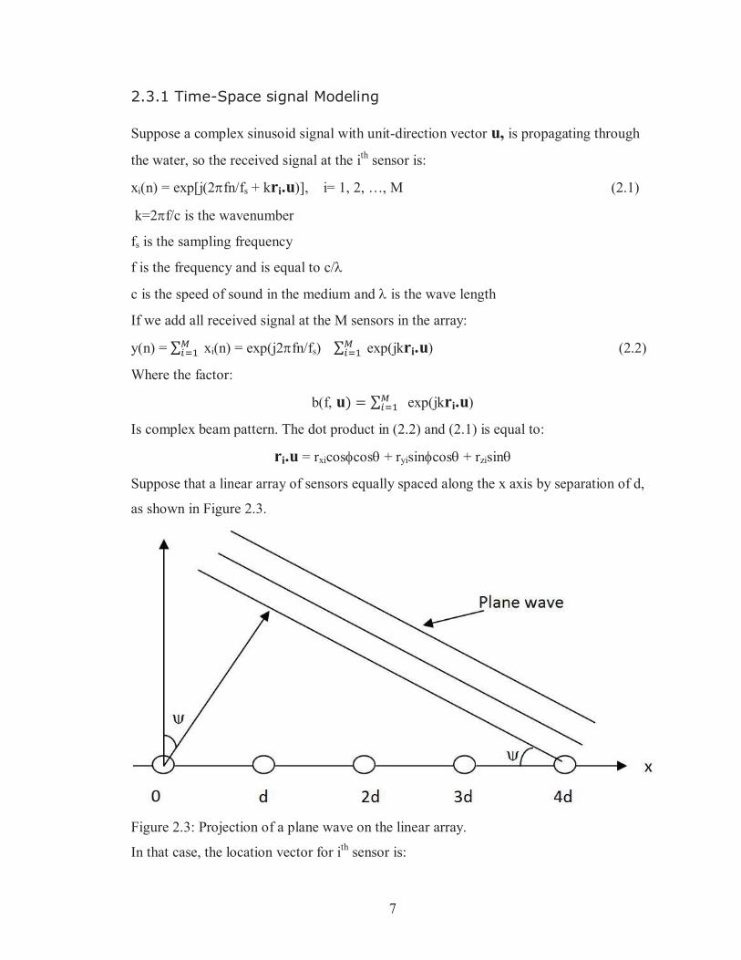
Suppose that a linear array of sensors equally spaced along the x axis by separation of d,
as shown in Figure 2.3.
Figure 2.3: Projection of a plane wave on the linear array.
In that case, the location vector for ith sensor is:
8
ri = (i-1)d , i = 1, 2, …, M
by considering this geometry, (2.2) could be:
y(n) = exp(j2 fn/fs) exp(jk(i-1)d cos cos ) (2. 3)
The conic angle , represent the projection of the plane wave signal with direction vector
u on the x axis and sin = cos cos as shown in Figure 2.3.
The magnitude of the summation (2.3) is:
sin[( fMd sin )/c]
|b(f, )| = (2.4) sin[( fd sin )/c]
Equation 2.4 represents the beam pattern of array. The beam power pattern is |b(f, )| 2.
According to the numerator and denominator that are function of sin for a given
frequency, a plane wave with a conic angle not equal to zero is attenuated. For conic
angle of = 0 degree all M sensors receive the plane wave simultaneously and the
outputs of these sensors could add in phase.
If we inspect the numerator of (2.4), it shows that the first zero crossings occur for ( fMd
sin )/c = ± , or = sin-1[c/(fMd)]. This area of the beam pattern called main lobe.
Main lob total area is inversely proportional to frequency f, to the number of sensors M
and to the sensor spacing d. The remaining region of the beam pattern called the side lobe
region [7].
2.3.2 Beam Steering Based on the existing time delay between the arrival signals on the sensors, we apply a
delay to the sensor outputs before performing the summation in (2.2). Without applying
the delay the response of the beamforming operation is maximum at = 00 and the plane
wave is parallel to the array. For an arbitrary direction vector, u0, if we want to add the
sensor signals coherently/in phase we have to calculate the projection of the vector, (u –
u0), on the ri (i = 1, 2, …, M) vectors.
9
For the three-dimensional case, (2.2) becomes:
y(n) = xi(n) = exp(j2 fn/fs) exp(jkri. (u – u0))
The beam pattern for equally spaced linear array is:
Sin[( fMd (sin sin )/c]
|b(f, )| = (2.5) Sin[( fd (sin sin )/c]
To form or steer a beam at angle , we have to apply the correct delay to each sensor
output. This kind of beam often called a synchronous beam.
2.3.3 Beamwidth
To calculate the required number of beams for spatial coverage, we have to determine the
3-dB beamwidth. We are interested in values of close to , so the equation (2.5)
becomes:
sin x
|b(f, )| = ,Where x = (fd/c) (sin sin
x Max |b(f, )| = M for . To find the 3dB, we can divide the maximum by √2 and
find the x:
(Max |b(f, )| )/√2 = M/√2 for x = ±0.44/M
Then sin 3dB = sin ±0.44/M and the beamwidth obtained by forming the difference of
two 3-dB angle [7]:
3dB ~ sin-1[sin + 0.44c/(Mfd)] – sin-1[sin – 0.44c/(Mfd)] (2.6)
2.4 ANALYSIS OF SPACE - TIME AND WAVENUMBER - FREQUENCY SIGNALS
In this section we model the linear array output signals as a function of space and time.
Then by applying the two dimensional Fast Fourier transform, we bring the signals from
time-space domain to frequency-wavenumber domain. Suppose that y(t, x) represent a
signal which is a function of time t and space x, then by the definition of the two
dimensional Fourier transform [10] [11]:
Y(k, exp[-j( t – k’x)] dt dx (2.7)

10
is the temporal frequency, and k represents the wavenumber vector which is the
number of wave per unit distance in each of the three orthogonal spatial directions. The
scalar term k’x is the dot product of the wavenumber vector k = (kx, ky, kz)’ and the
position vector x. If e(t, x) represents the propagated plane waves, then:
e(t, x) = exp [j( 0t – k’0x)] (2.8)
From the inverse 2D Fourier transform:
y(t, x Y(k, exp[-j( t – k’x)] dk d (2.9)
We can decomposed any signal y(t, x) into a superposition of propagated plane waves.
Figure 2-4 shows the k- space:
Figure 2.4: (k, ) space. (a) signals with a common frequency 0; (b) signals with a
common propagation speed; (c) signals with a common propagation direction.
kx kx
Ky Ky
Ky
|k| = c
kx/|k| = cos
(a) (b)
(c)
kx

11
2.4.1 Filtering in Frequency-Wavenumber Domain
In the beamforming algorithm, we work on signals with multivariable such as time and
space. Extracting signal components at specific frequencies and velocities of propagation
needs multidimensional filtering. We can separate the frequency components by applying
the 1D Fourier transform and then using a bandpass filter. Suppose that we send the Y(k,
signal (Equation 2.7) through a filter with an impulse response h(t, x) and the output
signal is f(t, x). The filter impulse response has to be designed to pass components of
interest (specific frequencies and velocities) and to reject those, such as additive noise
and/or propagation directions which we are not interested. The output and input of that
filter are related as a continuous convolution integral (in Time-Space domain) [10][11]:
f(t, x h(x – , t- y( , d d (2.10)
In the frequency-wavenumber domain, the output spectrum is equal to the product of the
input spectrum and the filter’s frequency-wavenumber response:
F(k, ) = H(k, ) Y(k, ) (2.11)
We must design the filter’s frequency-wavenumber response H(k, ) so that it is near
unity in the desired regions of (k, )-space and near zero in the other regions. If we want
to pass signal components in some narrow band around the specific frequency 0
independent of speed or direction of propagation, H(k, should have a 1D bandpass
frequency response which is independent of k [9].

12
2.4.2 Beamforming in Wavenumber – Frequency Domain Beamforming is a type of filtering that can be applied to signals carried by propagating
waves. The objective of a beamforming system is to isolate signal components that are
propagating in a specific direction and frequency. We assumed that the waves all
propagate with same speed c, so that the signals of interest is on the surface of the cone
=c|k| in (k, )-space. Ideally, the passband of the beamformer is the intersection of this
cone with the plane containing the desired direction vector (Figure 2.4 (c) ), as shown in
Figure 2.5.
Figure 2.5: Passband of an ideal beamformer. Passband of an ideal beamformer lies at
intersection of cone = c|k| and the plane containing the desired propagation direction
k0.
kx
Ky
13
2.5 WEIGHTED DELAY AND SUM BEAMFORMING
All mathematical models in the previous sections are based on weights with unity
magnitude. Now we are going to investigate the array weighting effects on beam patterns
(section 2.3) and DFT filter response (section 2.4.2).
2.5.1 Time domain Beamforming
In section 2.3 we calculated the complex beam pattern (Equation 2.4) for a linear array by
considering the propagation of a sinusoidal, ej2 fn/fs, plane wave in direction sin .
If we consider the weighting function ai, for ith sensor, then the beam pattern formula by
varying is [7]:
b(f, ) = aiexp[j2 f ( i – 1)d (sin – sin 0)/c] (2.11)
and by replacing i with i+1:
b(f, ) = ai+1exp[j2 fid (sin – sin 0)/c] (2.12)
Equation (2.4) represents the magnitude of the beam pattern for unity weight (ai = 1).
Let’s put Equation (2.2) which represents the output of sensors in a simple form:
y(t) = aixi(t – i) (2.13)
M represents the number of sensors, xi represents the sensor outputs, ai represents the
constant gains applied to the sensor outputs and i represents the time delays required to
point or steer the beam to the specified direction.
Figure 2.6 shows a time domain beamformer:

14
Time delay 1
Time delay 2
Time delay M
a1
a2
aM
x1(t) x
x2(t) x
Beam Output
xM(t) x
Figure 2.6: Time domain beamformer
The i called steering delays, compensate the differences in propagation times for the
individual array sensors. For the sources far enough away, the propagating signal is
considered as a plane wave and i are proportional to the projection of the sensor position
vector ri, relative to a reference point, onto a unit vector k in the direction of wave
propagation (refer to section 2.3). Usually the reference point has 0 = 0.
The ai, are spatial shading or weighting coefficients and are usually applied to the
individual sensors to adjust the spatial response or beam pattern received with the linear
array.
In the reference [13] and [14], some algorithms for synthesis of the weighting coefficients
are described, which give the ability to control the mainlobe width and sidelobe level.
The price for a reduction in the level of the sidelobes of the beam pattern is an increase in
the width of the mainlobe [15].

15
2.5.2 Frequency Domain Beamforming
Frequency domain beamforming has some advantages and disadvantages when compared
with time domain techniques. The most significant difference is that a time delay
transforms to a phase shift in the frequency domain [16].
The time delay in time domain is equal to a multiplication of the Fourier transform by e-
j t0 [11]:
f(t-t0) F( ) e-j t0
Frequency domain beamforming are merely the application of a Fourier transform to the
beamforming process. Because of the linearity of the beamforming process and properties
of the Fourier transform, the Fourier transform of the beam output is related with Fourier
transform of the sensor outputs as follows [15]:
By applying the Fourier transform on Equation (2.13)
Y(f, ) = ai (f) exp(-j2 f i( )) (2.14)
The Fourier transform of the beam output steered in direction , Y(f, ), is the weighted
linear combination of the Fourier transform of the received waveforms. In (2.14), the ai
represent the shading coefficient, the i( represent the delay required to steer the beam
in the direction , the phase shift , the 2 f i( are the frequency domain counterpart to
the time delays required for beam steering, and the Xi represent the Fourier transform of
the received waveform. One advantage is that the DFT can be computed efficiently and
fast by using a Fast Fourier Transform (FFT) algorithm [17][18]:

16
Fourier Transform
a1 e-j 1
Fourier Transform
a2 e-j 2
Fourier Transform
aM e-j M
Figure 2.7 depicted a simple frequency domain beamformer:
x1(t) x
x2(t) x
Y(f, )
xM(t) x
Figure 2.7: Frequency domain beamformer

17
CHAPTER 3 GPU COMPUTING
3.1 INTRODUCTION
“Computers are just as busy as the rest of us nowadays. They have a lot of tasks to do at
once and need some cleverness to get them all done at the same time.” [1].
GPU computing is the use of a GPU (Graphics Processing Unit) as a device together with
a CPU as a host to speed up scientific and engineering applications. In 2007 NVIDIA
presented GPU computing and it has quickly become an industry standard, used by
millions of scientist and engineers and adopted by almost all computing vendors.
GPU computing accelerates algorithms performance by executing compute-intensive part
of the application on the GPU, while the rest of the code runs on the CPU. In that case the
applications run faster.
CPU and GPU together, is a powerful combination. CPUs consist of a few cores designed
for sequential processing, and GPUs with thousands of efficient cores optimized for
parallel processing. Serial parts of the code execute on the CPU and parallel parts execute
on the GPU.
Intel Pentium family and the AMD Opteron family microprocessors based on a single
central processing unit (CPU), had significant progress by increasing the performance
ability and cost reductions for more than two decades.
GFLOPS (Giga FLoating-point Operations Per Second) has been brought to the desktop
and hundreds of GFLOPS to cluster servers by these microprocessors. Most software
developers, scientists and engineers have relied on the progress in hardware to accelerate
the speed of their algorithms. By introducing a new generation of processors, already
exist algorithms and applications runs faster. Due to power consumption issues, the
improvement of application’s speed has slowed since 2003. Regarding to the power
consumption issues, microprocessor vendors have switched to multi-core and many-core
systems.

18
Based on the human brain sequential style for solving problems and also available
sequential microprocessors, traditionally, most of the software applications are written as
sequential programs. From the other hand, computer users have the expectation that these
programs run faster with each new generation of microprocessors. This expectation is no
longer valid because a sequential program runs on just one of the processor cores, which
is not faster than those in use today.
Without using the parallel processing ability of multi cores systems, application
developers are not able to accelerate the applications by using new generation
microprocessors and it will reduce the growth opportunities of the entire computer
industry.
Instead, the parallel programmers will continue to enjoy performance improvement with
each new generation of microprocessors, in which multiple threads of execution
cooperate to accelerate applications.
Parallel programming is not new style in computer programming. The high performance
software developers have been creating parallel programs for decades. Those parallel
programs run on large scale, expensive computers. Large scale, expensive computers are
affordable just for limited applications and it will cause a significant limitation on the
practice of parallel programming.
“Now that all new microprocessors are parallel computers, the number of applications
that need to be developed as parallel programs has increased dramatically. There is now a
great need for software developers to learn about parallel programming” [2].
Since 2003, there is a race for floating-point performance between many-core processors
GPUs and multi-core CPUs vendors. Figure 3.1 shows this phenomenon. The GPUs
vendors continuously improve floating-point performance, while the performance
improvement of general purpose microprocessors has slowed significantly.
Based on the Figure 3.1 in 2009, the ratio of peak floating-point calculation throughput
between many-core GPUs and multi-core CPUs is about 10. NVIDIA has presented G80
Ultra to reach 518 GFLOPS, only about seven months after the original chip by
improving software driver and clock improvements. We used NVIDIA GeForce GTX
690 GPU (Figure 3.3) as a real-time digital beamformer, which delivers 2x2810.88

19
GFLOPS FMA (Fused Multiply-Add is an operation that performed in one step, with a
single rounding, which means calculating a+ (b*c) and then round it to N significant
bits).
Figure 3.1 Enlarging Performance Gap between GPUs and CPUs [2].
To understand such a large performance difference between many-core GPUs and CPUs
we have to understand the difference in fundamental design philosophy between the two
types of processors, as illustrated in Figure 3.2.

20
Figure 3.2 Fundamentally different design philosophies between CPU and GPU [2]. Memory bandwidth is another important subject in multi processors systems. Graphics
chips have been operating at approximately 10 times the bandwidth of available CPU
chips. In late 2006, G80 was capable of about 80 gigabytes per second (GB/S) into the
main DRAM. GeForce GTX 690 has 384 GB/S memory bandwidth [24].
Figure 3.3 GeForce GTX 690 GPU card from NVIDIA
21
3.2 COMPUTER UNIFIED DEVICE ARCHITECTURE (CUDA)
CUDA is a parallel computing platform and programming model invented by NVIDIA. It
enables dramatic increases in computing performance by harnessing the power of the
GPU. The GPU computing system consists of two parts. First part is a host which is CPU
side, such as Intel architecture microprocessor in personal computers, and the other part
is one or more devices which are parallel processors with a large number of Arithmetic
Logic Units (ALU). In scientific and engineering applications, there are usually program
sections that have rich amount of data parallelism, and it is a good opportunity to execute
many arithmetic operations safely on the program data structures in parallel manner. The
CUDA software accelerates the execution of these applications by using the GPU
computation ability to perform a large amount of data parallelism on the device side.
Since data parallelism plays such an important role in CUDA, in the next sections, we
will discuss the concept of data parallelism and basic features in CUDA.
3.2.1 CUDA Program Structure A CUDA program includes one or more phases that are executed on the host (CPU side)
and one or more phases that are executed on the device (GPU side).
To optimize the algorithm’s speed, we could implement the phases that have a little or no
data parallelism in the host code and implement the phases that have rich amount of data
parallelism in the device code.
The program includes a single source code for both host and device code. The NVIDIA C
Compiler nvcc separates the two source codes. The host code is ANSI C code. Host’s
standard C compilers compile host code and runs as an ordinary process. The device code
is written using ANSI C extended with some extra function and keywords for labeling
data-parallel functions, called kernels, and their associated data structures. The device
code is compiled by the nvcc and executed on a GPU device. It is possible to use the

22
emulation feature in CUDA, if there is no device available or the kernel is more
appropriately executed on a CPU.
The kernel functions usually generate a large number of threads to operate data
parallelism. Suppose that we want to multiply matrix A by matrix B element by element
and generate output matrix C (equal to “A .* B=C” operation in MATLAB), it can be
implemented as a kernel and use threads to compute one element of the output matrix. In
that case, the number of threads used by the kernel is equal to multiplication of the matrix
dimensions. For a two dimensional matrix 1000 by 1000 matrix multiplication, the kernel
that uses one thread to compute one output element would generate 1,000,000 threads.
These threads in CUDA program take very few cycles to generate and schedule because
of efficient GPU hardware structure while the CPU threads typically take thousands of
clock cycles to generate and schedule [2-4].
3.2.2 Kernel Functions and Threading
This section presents the CUDA kernel functions and the organizations of threads
generated by the kernel functions. In CUDA, a kernel function represents the code to be
executed on GPU side, by all threads in parallel. All threads of a parallel phase execute
the same code (Single-Program), so CUDA programming is an example of the Single-
Program Multiple-Data (SPMD) parallel programming style, which is an important
programming style in parallel computing systems.
Figure 3.4 shows the kernel function for element by element matrix multiplication. The
syntax is ANSI C with some extensions. There is a CUDA specific keyword
“__global__” in front of the declaration of MatrixMulKernel(). This keyword indicates
that the function is a kernel and that it can be called from a host and execute on the
device.
The second important extension to ANSI C is the keywords “threadIdx.x” and
“threadIdx.y”. These keywords refer to the thread configuration. Note that all threads
execute the same kernel code. We need a mechanism to allow threads to have access
toward the particular parts of the data structure that they are designated to work on.
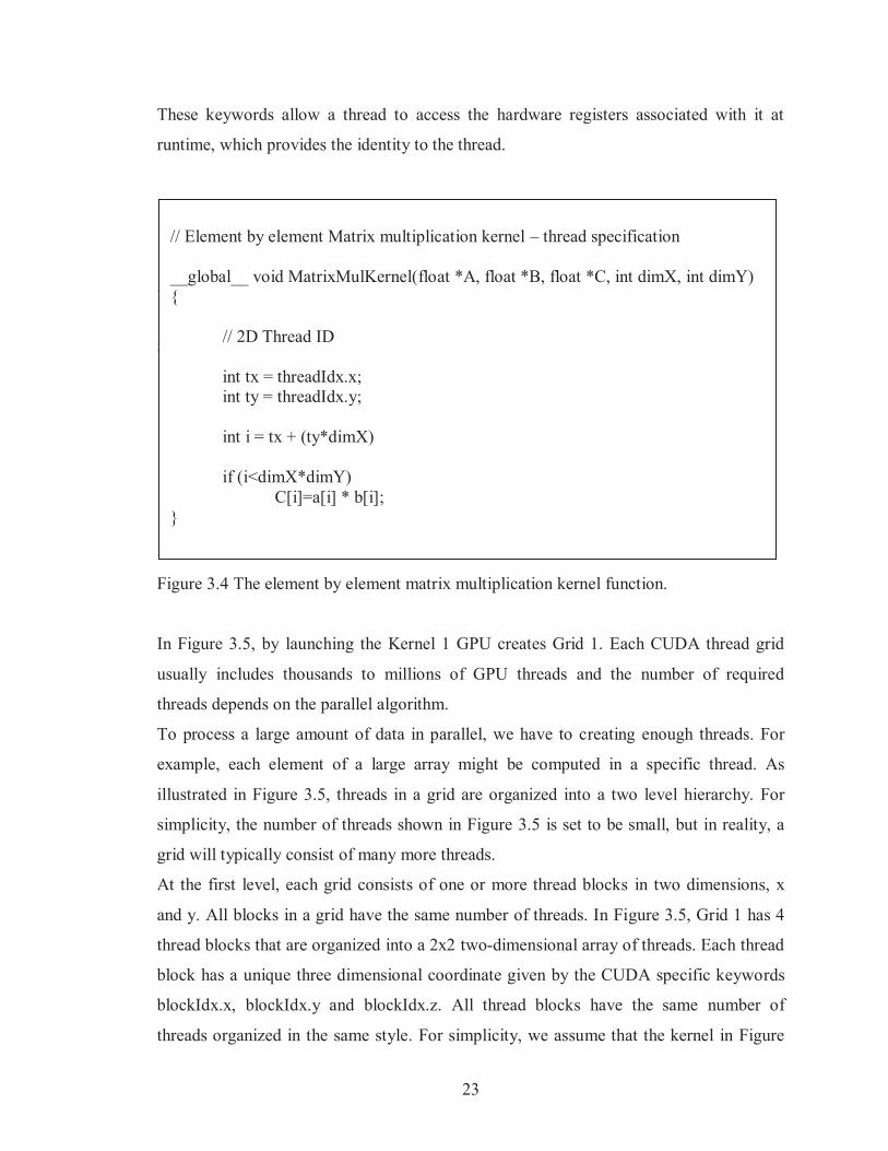
23
These keywords allow a thread to access the hardware registers associated with it at
runtime, which provides the identity to the thread.
3.3 CUDA THREADS
Section 3.2 is another subsection at the second level for the table of contents. For some
3.3.1 Thread Organization
3.3.2 CUDA General Algorithm Figure 3.4 The element by element matrix multiplication kernel function.
In Figure 3.5, by launching the Kernel 1 GPU creates Grid 1. Each CUDA thread grid
usually includes thousands to millions of GPU threads and the number of required
threads depends on the parallel algorithm.
To process a large amount of data in parallel, we have to creating enough threads. For
example, each element of a large array might be computed in a specific thread. As
illustrated in Figure 3.5, threads in a grid are organized into a two level hierarchy. For
simplicity, the number of threads shown in Figure 3.5 is set to be small, but in reality, a
grid will typically consist of many more threads.
At the first level, each grid consists of one or more thread blocks in two dimensions, x
and y. All blocks in a grid have the same number of threads. In Figure 3.5, Grid 1 has 4
thread blocks that are organized into a 2x2 two-dimensional array of threads. Each thread
block has a unique three dimensional coordinate given by the CUDA specific keywords
blockIdx.x, blockIdx.y and blockIdx.z. All thread blocks have the same number of
threads organized in the same style. For simplicity, we assume that the kernel in Figure
// Element by element Matrix multiplication kernel – thread specification __global__ void MatrixMulKernel(float *A, float *B, float *C, int dimX, int dimY) {
// 2D Thread ID int tx = threadIdx.x; int ty = threadIdx.y; int i = tx + (ty*dimX) if (i<dimX*dimY)
C[i]=a[i] * b[i]; }

24
3.4 is launched with only one thread block. A practical kernel will create much large
number of thread blocks.
Figure 3.5 CUDA thread organization.
Each thread block should be organized as a three dimensional array of threads with a total
number of up to 512 threads. The coordinates of threads in a block are uniquely defined
by three thread indices: threadIdx.x, threadIdx.y, and threadIdx.z. It depends on the
applications to use all the three dimensions of a thread block or just two/one of them. In
Figure 3.5, each thread block uses three dimensions and is organized into a 4x2x2 array
of threads. This gives Grid 1 a total of 4*16=64 threads. This is obviously a simple
example. In our beamforming algorithm, 128*32768*23=96,468,992 threads have been
used to multiply sensors output signals in wavenumber-frequency domain by k- filter.
The code in Figure 3.4 can use only one thread block organized as a 2-dimensional array
of threads in the grid. Also a thread block contains up to 512 threads and each thread is to
25
calculate one element of the product matrix, so the code can only calculate a product
matrix of up to 512 elements. This is of course not acceptable. If the product matrix needs
to have millions of elements to have sufficient amount of data parallelism to benefit from
execution on a device, we need multiple blocks.
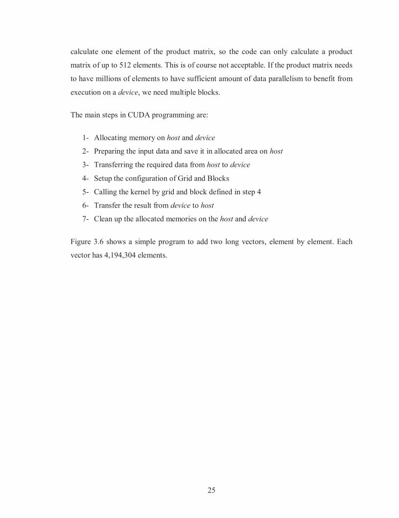
The main steps in CUDA programming are:
1- Allocating memory on host and device
2- Preparing the input data and save it in allocated area on host
3- Transferring the required data from host to device
4- Setup the configuration of Grid and Blocks
5- Calling the kernel by grid and block defined in step 4
6- Transfer the result from device to host
7- Clean up the allocated memories on the host and device
Figure 3.6 shows a simple program to add two long vectors, element by element. Each
vector has 4,194,304 elements.
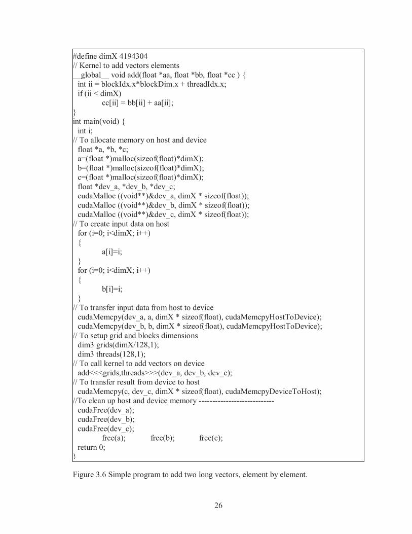
26
Figure 3.6 Simple program to add two long vectors, element by element.
#define dimX 4194304 // Kernel to add vectors elements __global__ void add(float *aa, float *bb, float *cc ) { int ii = blockIdx.x*blockDim.x + threadIdx.x; if (ii < dimX) cc[ii] = bb[ii] + aa[ii]; } int main(void) { int i; // To allocate memory on host and device float *a, *b, *c; a=(float *)malloc(sizeof(float)*dimX); b=(float *)malloc(sizeof(float)*dimX); c=(float *)malloc(sizeof(float)*dimX); float *dev_a, *dev_b, *dev_c; cudaMalloc ((void**)&dev_a, dimX * sizeof(float)); cudaMalloc ((void**)&dev_b, dimX * sizeof(float)); cudaMalloc ((void**)&dev_c, dimX * sizeof(float)); // To create input data on host for (i=0; i<dimX; i++) { a[i]=i; } for (i=0; i<dimX; i++) { b[i]=i; } // To transfer input data from host to device cudaMemcpy(dev_a, a, dimX * sizeof(float), cudaMemcpyHostToDevice); cudaMemcpy(dev_b, b, dimX * sizeof(float), cudaMemcpyHostToDevice); // To setup grid and blocks dimensions dim3 grids(dimX/128,1); dim3 threads(128,1); // To call kernel to add vectors on device add<<<grids,threads>>>(dev_a, dev_b, dev_c); // To transfer result from device to host cudaMemcpy(c, dev_c, dimX * sizeof(float), cudaMemcpyDeviceToHost); //To clean up host and device memory ---------------------------- cudaFree(dev_a); cudaFree(dev_b); cudaFree(dev_c); free(a); free(b); free(c); return 0; }

27
By using MacBook Air laptop under Mac OS X, Version 10.6.8 with NVIDIA
GeForce 320M GPU, the add kernel in Figure 3.6 needs 0.000157 Sec. to calculate the
result, but if we just use CPU, it needs 0.0589 Sec., which means that the GPU
computation is faster than CPU sequential more than 402 times. Refer to Chapter 5,
section 5.2 for more GPU computation and CPU sequential usage time and speed
comparison.

28
CHAPTER 4 PARALLEL SONAR SIGNAL PROCESSING
4.1 INTRODUCTION
Sonar beamforming algorithms can require on the order of billions of multiply
accumulates (MACs) per second and therefore have traditionally been implemented in
custom hardware [20].
Based on the detailed explanation of beamforming in Chapter 2, the objective of
beamforming is to align the signals arriving at the linear array of sensors from a certain
direction in time/phase, so that they can be added coherently. This means that signals
coming from all other directions will be added incoherently, and as a consequence
attenuated. The bulk of the operations required for beamforming are parallel intensive
tasks. These include: matrix multiplication, zero padding, filtering, FFT and IFFT. In this
thesis I described the use of GPU as a digital beamformer and compare the speed of
calculation between two methods:
1. Beamforming by GPU
2. Beamforming by CPU
Figure 4.1 depicted the main algorithm for digital beamforming by GPU computing.

29
Start
Figure 4.1: Main algorithm for digital beamforming by GPU computing
Preparing data and parameters
Zero padding
1D IFFT on space domain to bring data from Wavenumber-Frequency (k- ) domain to Space-Frequency domain (x- )
Apply time delay mask in x- domain
2D (Space-Time) filtering (k- Masking)
End
2D FFT to bring data from Space-Time domain (x-t) to Wavenumber-Frequency (k- ) domain
Add sensors output to calculate beamformer output
1D IFFT on time domain to bring data from Space-Frequency (x- ) domain to Space-Time domain (x-t)

30
4.2 PREPARING DATA AND PARAMETERS
Synthetic data has been generated to test the proposal sonar processing. This data
simulates a plane wave insonifying a 64 sensors array in presence of white Gaussian
Noise and array self noise (very low speed “bulge” wave propagating along the array).
We consider the case of 64 sensors in a linear array of equally spaced along the x axis
with a separation of d = 0.10 m as shown in Figure 4.1.
d=0.10m
x
0 d 2d 62d 63d
Array length = 6.3 m
Figure 4.2: Geometry of a linear array of equally spaced sensors
As shown in Figure 4.2, the array length is equal to 63 * 0.10 m = 6.3 m
Each sensor works as an input channel (ch1 – ch64) and receives N = 10*1024=16,384
samples per each inspection period.
The sound speed in sea-water is taken as c = 1470 m/Sec.
The sampling frequency Fs is 11025 Hz, with a time period between two samples of:
t = 1/Fs = 1/11025 = 9.0703e-05 Sec.
By considering the number of samples, 16384, the length of inspection period is:
Inspection period length = t * N = 9.0703e-05 Sec. * 16384 = 1.4861 Sec.
Based on this calculation Figure 4.3 depicts the data matrix y (64 Sensors output) in
Time-Space domain:
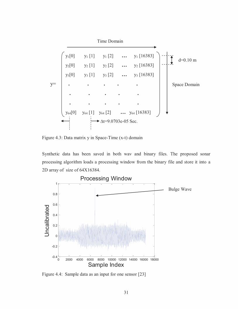
31
y1[0] y1 [1] y1 [2] … y1 [16383]
y2[0] y2 [1] y2 [2] … y2 [16383]
y3[0] y3 [1] y3 [2] … y3 [16383]
y= . . . . .
. . . . .
. . . . .
y64[0] y64 [1] y64 [2] … y64 [16383]
t=9.0703e-05 Sec.
Figure 4.3: Data matrix y in Space-Time (x-t) domain
Synthetic data has been saved in both wav and binary files. The proposed sonar
processing algorithm loads a processing window from the binary file and store it into a
2D array of size of 64X16384.
Figure 4.4: Sample data as an input for one sensor [23]
0 2000 4000 6000 8000 10000 12000 14000 16000 18000-0.4
-0.2
0
0.2
0.4
0.6
0.8
1Processing Window
Sample Index
Unc
alib
rate
dTime Domain
Space Domain
d=0.10 m
Bulge Wave
32
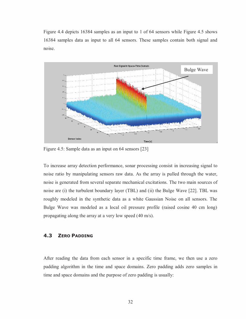
Figure 4.4 depicts 16384 samples as an input to 1 of 64 sensors while Figure 4.5 shows
16384 samples data as input to all 64 sensors. These samples contain both signal and
noise.
Figure 4.5: Sample data as an input on 64 sensors [23]
To increase array detection performance, sonar processing consist in increasing signal to
noise ratio by manipulating sensors raw data. As the array is pulled through the water,
noise is generated from several separate mechanical excitations. The two main sources of
noise are (i) the turbulent boundary layer (TBL) and (ii) the Bulge Wave [22]. TBL was
roughly modeled in the synthetic data as a white Gaussian Noise on all sensors. The
Bulge Wave was modeled as a local oil pressure profile (raised cosine 40 cm long)
propagating along the array at a very low speed (40 m/s).
4.3 ZERO PADDING
After reading the data from each sensor in a specific time frame, we then use a zero
padding algorithm in the time and space domains. Zero padding adds zero samples in
time and space domains and the purpose of zero padding is usually:
Bulge Wave
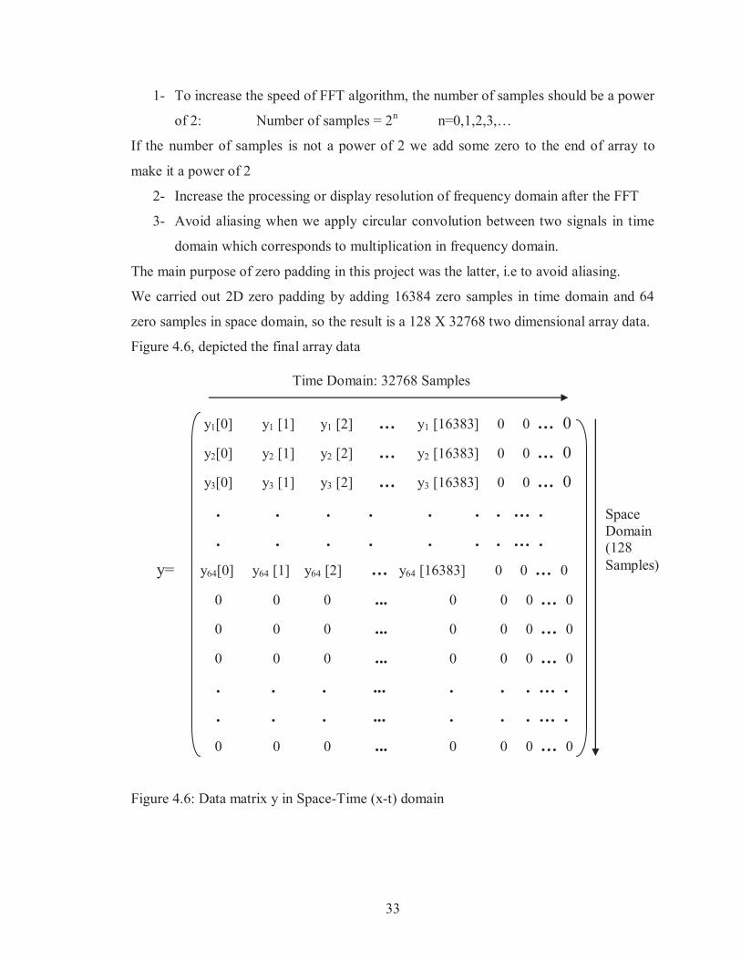
33
Space Domain (128 Samples)
1- To increase the speed of FFT algorithm, the number of samples should be a power
of 2: Number of samples = 2n n=0,1,2,3,…
If the number of samples is not a power of 2 we add some zero to the end of array to
make it a power of 2
2- Increase the processing or display resolution of frequency domain after the FFT
3- Avoid aliasing when we apply circular convolution between two signals in time
domain which corresponds to multiplication in frequency domain.
The main purpose of zero padding in this project was the latter, i.e to avoid aliasing.
We carried out 2D zero padding by adding 16384 zero samples in time domain and 64
zero samples in space domain, so the result is a 128 X 32768 two dimensional array data.
Figure 4.6, depicted the final array data
y1[0] y1 [1] y1 [2] … y1 [16383] 0 0 … 0
y2[0] y2 [1] y2 [2] … y2 [16383] 0 0 … 0
y3[0] y3 [1] y3 [2] … y3 [16383] 0 0 … 0
. . . . . . . … .
. . . . . . . … .
y= y64[0] y64 [1] y64 [2] … y64 [16383] 0 0 … 0
0 0 0 ... 0 0 0 … 0
0 0 0 ... 0 0 0 … 0
0 0 0 ... 0 0 0 … 0
. . . ... . . . … .
. . . ... . . . … .
0 0 0 ... 0 0 0 … 0
Figure 4.6: Data matrix y in Space-Time (x-t) domain
Time Domain: 32768 Samples

34
To accelerate the speed of zero padding algorithm, we used a CUDA kernel to do zero
padding on the GPU. Refer to Chapter 5 for a detailed explanation speed comparison
between CPU sequential and GPU computation.
4.4 2D FFT ON TIME-SPACE DOMAIN
Following the method provided in section 2.4.1 “Filtering in Wavenumber - Frequency
Domain” If we are interested in extracting signal components at specific frequencies and
velocities of propagation, then we can separate the frequency components by applying a
Fourier transform and then using a bandpass filter. By applying a 2D FFT on the original
data array X, we bring data from the Space-Time domain (x-t) to Wavenumber-
Frequency (k- ) domain and subsequently carry out a k- analyses.
y array data is 2D array and has 128X32768 = 4,194,304 samples. 2D FFT(X) function
requires a lot of calculation and requires a lot of time, so it is a good opportunity to use
CUDA functions and apply 2D FFT to increase the speed of calculation by using parallel
processing resources on GPU. Refer to Chapter 5 for detail explanation about speed
comparison between CPU sequential and GPU computation. Figure 4.7 shows the raw
data in k- domain after 2D FFT.
Figure 4.7: Raw signal in k- domain [23]

35
4.5 SPATIAL FILTERING (K- MASKING)
The first step was to decide on the number of beams needed to satisfy the required
resolution of the full 360o space around the linear array. Based on the geometry of the
linear array, we need to scan just the space between -90 o to 90 o.
To calculate the beams, we divided the space between -90o to 90o into 23 regions
uniformly distributed in sin ( ) space (which means dividing the space [-1, 1] to 23 equal
subspace) with a 3dB maximum scalloping loss. For detail explanation refer to chapter 2,
section 2.3.3. Figure 4.8 depicted the beam level between [-90o and 90o].
Figure 4.8: 23 Array beams uniformly distribution on sin ( ) [23]
In the second step we created a two dimensional filter (k- Mask) for each individual
beam and multiply it in the k- domain by the sensors’ outputs (Equation 4.2) to reject
unnecessary data. Based on explanation in section 2.4 and Equation (2.7):
-80 -60 -40 -20 0 20 40 60 80-6
-5
-4
-3
-2
-1
0
Angle (Deg.)
Bea
m L
evel

36
Y(k, = 2D FFT [y(x, t)] (4.1) We are looking for a filter with an impulse response h(t, x) to pass components of interest
and to reject things like additive noise and/or propagation directions which we are not
interested (Refer to Equation 2.10 for relation between output and input of that filter).
So in the Wavenumber - Frequency domain, the output spectrum is equal to the product
of the input spectrum and the filter’s Wavenumber - Frequency response:
F(k, ) = H(k, ) Y(k, ) (4.2)
We used a Gaussian window (along wavenumber axis) extended along the frequency axis
to define a 2D Beam Filter Mask. An example of such a mask is presented in Figure 4.9
for a beam steering angle of 46.6582o.
Figure 4.9: k – Filter Mask for beam angle = 46.6582o [23]
Figure 4.10 depicted the result of multiplication of sensors’ outputs by k– filter mask in
Time – Space domain and Figure 4.11 depicted the result in Wavenumber - Frequency
domain. Figure 4.12 shows the raw data and filtered data (for beam steering angle =

37
46.6582o) on one sensor. After filtering, there is no unnecessary data, so it is much easier
to analyze.
Figure 4.10: Filtered signal in Space – Time domain for beam angle = 46.6582o [23]
Figure 4.11: Filtered signal in k- domain for beam angle = 46.6582o [23]

38
Figure 4.12: Raw data and filtered data on one sensor for steering beam = 46.6582o [23]
We need to create or read the k– filter mask just one time and use it when we have a
new set of data.
Based on explanation about 23 steering beams in the beginning of this section, we have to
multiply a 2D array with 128 x 32768 complex elements by k-w masking 2D array with
128 x 32768 real elements, 23 times. It means 128 x 32768 x 23 = 96,468,992
multiplications for real parts and 96,468,992 multiplications for imaginary parts, which is
totally 192,937,984 multiplications. To accelerate the speed of k– masking algorithm,
we used a kernel to do k– masking as a parallel process in GPU. Refer to Chapter 5 for
detail explanation about speed comparison between CPU sequential and GPU
computation.
39
4.6 TIME DELAY MASK
Based on explanation in Chapter 2, Sec 2.5.2 “Frequency Domain Beamforming” and
Figure 2.7, in the first step we have to bring data to the frequency domain and then
multiply required coefficient to compensate the existing time delay between sensors. In
this stage, because of 2D FFT in the last stage, our data in GPU is in the k- domain. To
bring the data in Space-Frequency domain (x- ), we have to apply 1D IFFT on
wavenumber domain. Then in the second step we need to create or read the time delay
filter mask just one time and use it when we have a new set of data. In the last step we
have to multiply the data by time delay mask, which is a complex multiplication of two
2D matrixes element by element. To accelerate the speed of time delay masking
algorithm, we used 1D IFFT function in CUDA to apply 1D IFFT algorithm as a parallel
process in GPU. Based on explanation about 23 steering beams in the beginning of
section 4.5, we have to multiply a 2D array with 128 x 32768 x 23 complex elements by
time delay masking 2D array with 128 x 32768 x 23 complex elements. Consider the
following complex multiplication:
x = a + ib
y = c + id
a . b = ((a * c) - (b * d)) + i((a * d) + (b * c))
For each complex multiplication we need four multiplications and three additions. It
means 128 x 32768 x 23 x 4 = 385,875,968 multiplications and 128 x 32768 x 23 x 3 =
289,406,976 additions. We used a kernel to apply the time delay mask as a parallel
process in GPU. Refer to Chapter 5 for detail explanation about speed comparison
between CPU sequential and GPU computation.

40
Space Domain (128 Samples)
4.7 SUMMATION
In this stage, there is no time delay between sensors’ outputs and the signal is in the
Space-Frequency (x- ) domain. In first step we have to apply 1D IFFT in frequency
domain to bring data in Space-Time domain (x-t). In the second step we have to add all
sensors’ outputs for each individual samples in the time domain (Summation algorithm).
Figure 4.13 shows the mathematical procedure:
y1[0] y1 [1] y1 [2] … y1 [32768]
+ + + + +
y2[0] y2 [1] y2 [2] … y2 [32768]
+ + + + +
y= y3[0] y3 [1] y3 [2] … y3 [32768]
+ + + + +
. . . … . + + + + +
y128[0] y128 [1] y128 [2] … y128 [32768]
y= y[0] y [1] y [2] … y [32768]
Figure 4.13: Summation procedure for each steering angle.
To accelerate the speed of time delay masking algorithm, we used 1D IFFT function in
CUDA to apply 1D IFFT algorithm as a parallel process in GPU. Based on explanation
about 23 steering beams in the beginning of section 4.5, we have to add 128 1D arrays
Time Domain: 32768 Samples

41
with 32768 elements, 23 times, which means 128 x 32768 x 23 = 96,468,992 additions.
We used a kernel to apply summation algorithm as a parallel process in GPU. Refer to
Chapter 5 for detail explanation about speed comparison between CPU sequential and
GPU computation. Figure 4.14 shows the result after applying time delay masking.
Figure 4.14: Filtered and time delayed signal in k- domain [23]
Figure 4.15 shows the raw data on one sensor and beamformer output (signal after
applying summation algorithm).
Figure 4.15: Raw data on one sensor and beamformer output [23]
42
CHAPTER 5 RESULTS
5.1 BEAMFORMING BY CPU SEQUENTIAL AND GPU COMPUTATION
In this thesis we applied beamforming algorithms by CPU sequential (MATLAB code)
and GPU Computation (CUDA code) algorithms on the same computer and proved that,
we could accelerate the speed of signal processing by applying parallel processing
technique by using the GPU as digital beamformer. Based on explanation in Chapter 4
and the flow chart depicted in Figure 4.1, our beamforming algorithm has some main
functions which are in the first column of Table 1. Table 5.1: Time usage comparison between MATLAB code and CUDA code
Function MATLAB Code Time
Usage (mSec.)
CUDA Code
Time Usage
(mSec.)
CUDA is
Faster
(Times)
One Steering
Angle
23 Steering
Angles
23 Steering
Angles
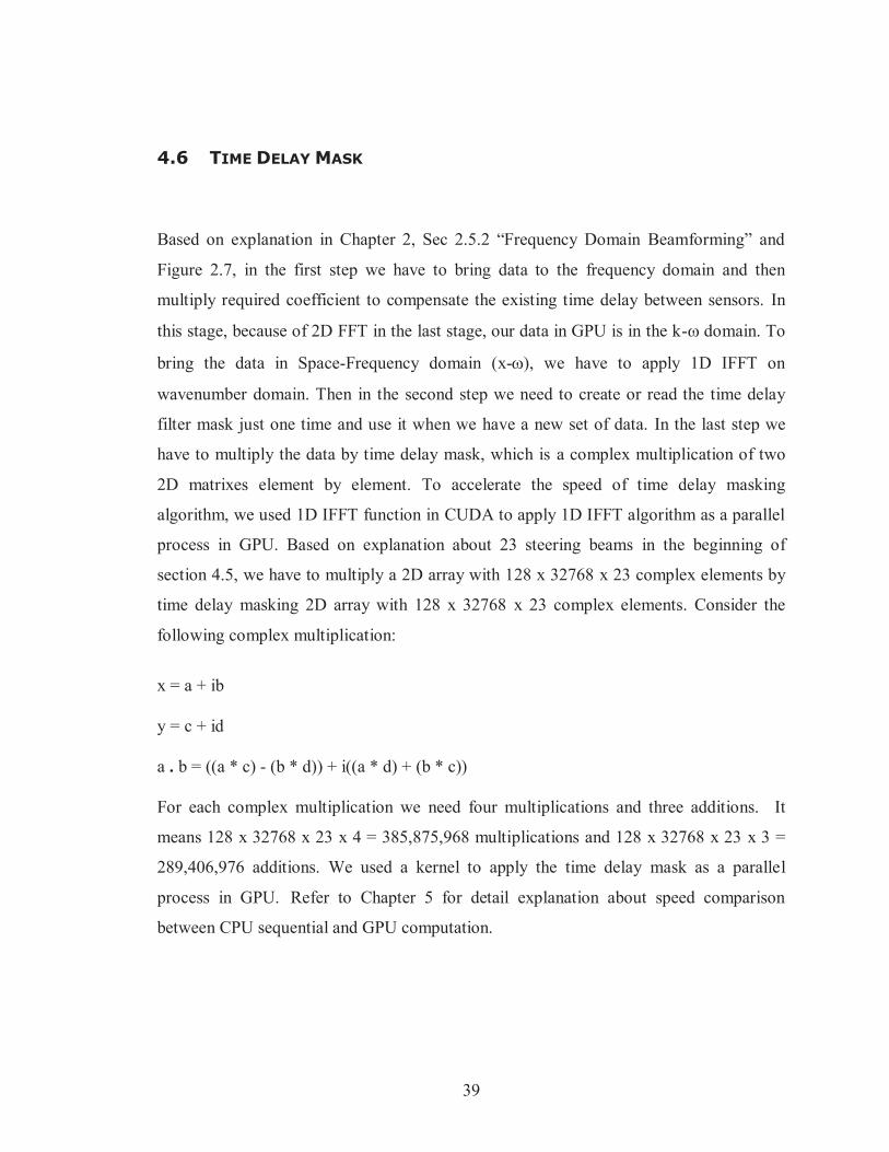
Reading array data 12.5 12.5 2.5 5 Zero Padding 14.3 14.3 20.03 0.71 2D FFT 278.5 278.5 0.6 464.17 K- Masking 29.6 680.8 114.72 5.93 1D IFFT on Space Domain 110 2530 1.56 1621.79 Time Delay Masking 34.5 793.5 217.76 3.64 1D IFFT on Time Domain 241.8 5561.4 339.56 16.38 Summation 11.3 259.9 0.25 1039.6 Total: 732.5 10130.9 696.98 14.54
Second and third columns show the MATLAB code usage time to apply beamforming for
one steering angle and 23 steering angles. Fourth column shows the CUDA usage time
for 23 steering angles. Fifth column shows that, how much CUDA is faster than
MATLAB (Dividing the MATLAB usage time by CUDA usage time for 23 steering
angles). In MATLAB code, to complete all 23 steering angles for a set of data, we have
to execute Reading Data, Zero Padding and 2D FFT functions, just one time and the rest

43
of functions, 23 times. But in CUDA code, based on parallel processing nature of
algorithm we could execute all functions in the same time for all 23 steering angles.
According to the abstract, the objective of this thesis is to use Graphics Processing Unit
(GPU) as real-time digital beamformer to accelerate the intensive signal processing. The
sections 5.1.2 and 5.1.3, explain the results based on the objective of this thesis.
5.1.1 Using GPU As A Beamformer We used GPU computation (CPU + GPU) to process the received signal from the sensors
as a beamformer. By this way we did not use expensive custom design beamformer.
5.1.2 Real-Time Beamformer
According to the Table 1, total usage time to run required beamforming algorithms by
MATLAB code is 10.131 Sec. and by CUDA code is 0.697 Sec., which means CUDA
code is 14.54 times faster.
In Section 4.2 we explained that the inspection period length (Data length) is 1.4861 Sec.
and the required time to apply beamforming algorithms by CUDA is 0.697 Sec., which
means, after receiving the first batch of data with length of 1.4861 Sec. we could process
it in 0.697 Sec. and beamforming algorithms are completely done before we get next
batch of data, so it is a real-time processing and is one of the main goals of beamforming.
5.1.3 Accuracy Another subject that we have to address is generated errors by algorithms. From a
practical point of view, MATLAB code or CUDA code generates some errors, when we
apply some algorithms (For example, FFT or IFFT), but the question is, what is the
maximum difference between MATLAB code and CUDA code results?
Via numerical result, after calculating the maximum difference between MATLAB code
and CUDA code results is 3.05474e -07, which is negligible when we compare it with
already exist noises or errors generated by the hardware.

44
By this way, we showed that GPU computing has the ability to perform the beamforming
algorithms with enough accuracy as a real-time system and it is available on the personal
computers, so there is no need to spend time and money for custom design beamformer
hardware.
45
CHAPTER 6 CONCLUSION
6.1 CPU SEQUENTIAL AND GPU COMPUTATION COMPARISON In this section we compare the CPU sequential and GPU computation usage time and
speed for some popular functions. Before starting to explain each function, let’s have a
closer look at execution of a kernel on GPU. Each execution has three main parts:
1. Transfer data from CPU (Host) side to GPU (Device) side
2. Execute the kernel on GPU
3. Transfer the result from GPU side to CPU side
Figure 6.1 shows the block diagram of that sequence. Total usage time to execute just one
kernel is equal to TCToG1 + TExe1 + TGToC1.
Figure 6.1: Usage time to execute just on kernel on GPU
Suppose that we want to execute more than one kernel on GPU as a serial functions. In
that case after executing the first kernel, we don’t need to transfer result from GPU side
to CPU side and then transfer it again from CPU to GPU for next kernel execution.
Instead of that we could keep the result in GPU and execute the next kernel and so on. By
this way we can save a lot of time by avoiding transfer data between GPU and CPU and
the total usage time to execute n kernel is equal to:
Total Usage Time = TCToG1 + TExe1 + TExe2 + … + TExen + TGToCn
So the total usage is almost the execution of kernels on GPU if we avoid transferring data
between CPU and GPU. In our beamforming algorithms, we transfer a bath of new data
to GPU and then we execute the Zero Padding, 2D FFT, k-w Masking, 1D IFFT, Time
Delay Masking and Sensors’ Outputs Summation kernels. Via numerical results in Table
1, we have to transfer data from CPU to GPU one time with usage time = 0.002397 Sec.
Transfer data from
CPU (Host) side to
GPU (Device) side.
Usage Time = TCToG1
Execute the kernel
on GPU.
Usage Time = TExe1
Transfer the result
from GPU side to CPU
side.
Usage Time = TGToC1

46
(0.35% of total usage time) and then apply the above beamforming kernels with usage
time = 0.6773 Sec. (99.65% of total usage time).
Suppose that we have a 2D array with N x M samples (N columns and M rows). Table 2
shows the CPU sequential and GPU computation usage time to apply 2D FFT, 2D IFFT,
1D FFT, 1D IFFT, Zero Padding and Summation functions for different values of N and
M. Based on the above explanations, all GPU usage times are the required time to
execute kernel on GPU and transferring data (between GPU and CPU) are not included.
Table 3 shows, how much GPU computation is faster (Times) by dividing CPU
sequential usage time by GPU computation usage time.
Table 6.1: CPU sequential and GPU computation usage times
Function Number of Samples (N x M)
4 k 1 M 2 M 4 M 8 M 16 M 64 M
2D FFT CPU Seq. 0.325 51 104.5 230.4 490.9 1,053 4,462.8
2D FFT GPU Com. 0.227 0.646 0.646 0.688 0.849 0.867 1.363
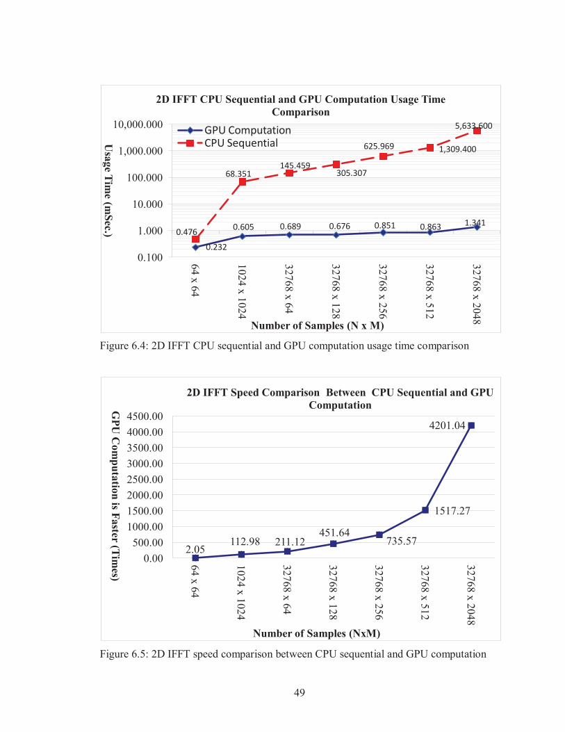
2D IFFT CPU Seq. 0.476 68.351 145.459 305.307 625.969 1,309.4 5,633.6
2D IFFT GPU Com. 0.232 0.605 0.689 0.676 0.851 0.863 1.341
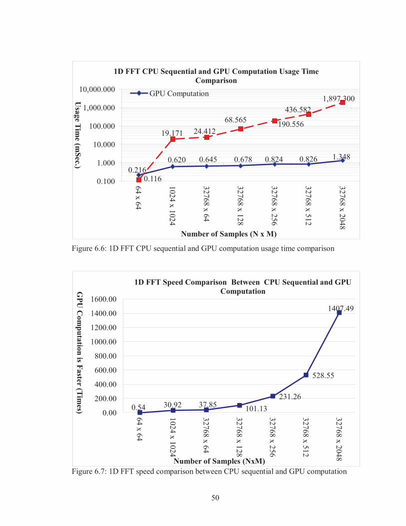
1D FFT CPU Seq. 0.116 19.171 24.412 68.565 190.556 436.582 1,897.3
1D FFT GPU Com. 0.216 0.62 0.654 0.678 0.824 0.826 1.348
1D IFFT CPU Seq. 0.212 42.248 67.671 151.787 321.431 698.744 3,143.6
1D IFFT GPU Com. 0.219 0.636 0.662 0.680 0.850 0.856 1.357
Zero Pad. CPU Seq. 0.029 1.697 6.471 14.402 26.940 53.242 203.51 Zero Pad. GPU Com. 0.023 0.025 0.025 0.028 0.040 0.045 0.045 Summation CPU Seq. 0.025 0.898 1.790 3.534 6.972 13.857 55.014 Summation GPU Com. 0.032 0.057 0.051 0.054 0.056 0.058 0.059

47
Table 6.2: Speed comparison between CPU sequential and GPU computation
Function Number of Samples (N x M) 4 k 1 M 2 M 4 M 8 M 16 M 64 M
1D FFT 0.54 30.92 37.85 101.13 231.26 528.55 1407.49 1D IFFT 0.97 66.43 102.22 223.22 378.15 816.29 2316.58 2D FFT 1.43 78.95 161.76 334.88 578.21 1214.53 3274.25 2D IFFT 2.05 112.98 211.12 451.64 735.57 1517.27 4201.04
Zero Padding 1.26 67.88 258.84 514.36 673.50 1183.16 4522.42 Summation 0.78 15.75 35.10 65.44 124.50 238.91 932.44
For the Zero Padding function, the original dimensions of input array is N/2 by M/2 and
we apply zero padding to double the dimensions by adding some zeros to the end of each
row and column (Refer to Figure 4.6 for N = 32768 and M = 128 example).
For Summation function, input array has N x M dimensions and we have to add all
samples in each column and save it in an array with dimension N x 1 (Refer to Figure
4.12 for N = 32768 and M = 128 example).
Figure 6.2 to 6.13 depicted the logarithmic graphs of the CPU sequential and GPU
computation usage time and speed comparison for each function.
Via the numerical data in Table 1, 2 and 3 and also the graphs, the major accomplishment
of GPU computation is the processing of massive data. When the number of samples is
low (for example 64 x 64), there is no significant difference between CPU sequential and
GPU computation, but by increasing the number of data, CPU sequential requires a lot of
usage time, however GPU computation usage time is almost flat and doesn’t change a lot.
We believe that parallel processing plays a major role in massive data processing and in
near future it has a significant role in scientific researches and based on the advantages of
GPU computation, which we explained in Section 1.1, it could be a powerful and not
expensive tool for scientists.

48
Figure 6.2: 2D FFT CPU sequential and GPU computation usage time comparison
Figure 6.3: 2D FFT speed comparison between CPU sequential and GPU computation
1.43 78.95 161.76
334.88 578.21
1214.53
3274.25
0.00
500.00
1000.00
1500.00
2000.00
2500.00
3000.00
3500.00
64 x 64
1024 x 1024
32768 x 64
32768 x 128
32768 x 256
32768 x 512
32768 x 2048
GPU
Com
putation is Faster (Times)
Number of Samples (NxM)
2D FFT Speed Comparison Between CPU Sequential and GPU Computation
0.227
0.646 0.646 0.688 0.849 0.867 1.363
0.325
51.000 104.500
230.400 490.900
1,053.000 4,462.800
0.100
1.000
10.000
100.000
1,000.000
10,000.000
64 x 64
1024 x 1024
32768 x 64
32768 x 128
32768 x 256
32768 x 512
32768 x 2048
Usage Tim
e (mSec.)
Number of Samples (N x M)
2D FFT CPU Sequential and GPU Computation Usage Time Comparison
GPU Computation CPU Sequential
49
Figure 6.4: 2D IFFT CPU sequential and GPU computation usage time comparison
Figure 6.5: 2D IFFT speed comparison between CPU sequential and GPU computation
0.232
0.605 0.689 0.676 0.851 0.863 1.341 0.476
68.351 145.459
305.307
625.969 1,309.400
5,633.600
0.100
1.000
10.000
100.000
1,000.000
10,000.000
64 x 64
1024 x 1024
32768 x 64
32768 x 128
32768 x 256
32768 x 512
32768 x 2048
Usage Tim
e (mSec.)
Number of Samples (N x M)
2D IFFT CPU Sequential and GPU Computation Usage Time Comparison
GPU Computation CPU Sequential
2.05 112.98 211.12
451.64 735.57
1517.27
4201.04
0.00 500.00
1000.00 1500.00 2000.00 2500.00 3000.00 3500.00 4000.00 4500.00
64 x 64
1024 x 1024
32768 x 64
32768 x 128
32768 x 256
32768 x 512
32768 x 2048
GPU
Com
putation is Faster (Times)
Number of Samples (NxM)
2D IFFT Speed Comparison Between CPU Sequential and GPU Computation
50
Figure 6.6: 1D FFT CPU sequential and GPU computation usage time comparison
Figure 6.7: 1D FFT speed comparison between CPU sequential and GPU computation
0.216 0.620 0.645 0.678 0.824 0.826 1.348
0.116
19.171 24.412 68.565 190.556
436.582 1,897.300
0.100
1.000
10.000
100.000
1,000.000
10,000.000
64 x 64
1024 x 1024
32768 x 64
32768 x 128
32768 x 256
32768 x 512
32768 x 2048
Usage Tim
e (mSec.)
Number of Samples (N x M)
1D FFT CPU Sequential and GPU Computation Usage Time Comparison
GPU Computation
0.54 30.92 37.85 101.13 231.26
528.55
1407.49
0.00
200.00
400.00
600.00
800.00
1000.00
1200.00
1400.00
1600.00
64 x 64
1024 x 1024
32768 x 64
32768 x 128
32768 x 256
32768 x 512
32768 x 2048
GPU
Com
putation is Faster (Times)
Number of Samples (NxM)
1D FFT Speed Comparison Between CPU Sequential and GPU Computation

51
Figure 6.8: 1D IFFT CPU sequential and GPU computation usage time comparison
Figure 6.9: 1D IFFT speed comparison between CPU sequential and GPU computation
0.219 0.636 0.662 0.680 0.850 0.856
1.357
0.212
42.248 67.671 151.787
321.431 698.744
3,143.600
0.100
1.000
10.000
100.000
1,000.000
10,000.000
64 x 64
1024 x 1024
32768 x 64
32768 x 128
32768 x 256
32768 x 512
32768 x 2048
Usage Tim
e (mSec.)
Number of Samples (N x M)
1D IFFT CPU Sequential and GPU Computation Usage Time Comparison
GPU Computation CPU Sequential
0.97 66.43 102.22
223.22 378.15
816.29
2316.58
0.00
500.00
1000.00
1500.00
2000.00
2500.00
64 x 64
1024 x 1024
32768 x 64
32768 x 128
32768 x 256
32768 x 512
32768 x 2048
GPU
Com
putation is Faster (Times)
Number of Samples (NxM)
1D IFFT Speed Comparison Between CPU Sequential and GPU Computation

52
Figure 6.10: Zero Padding CPU sequential and GPU computation usage time comparison
Figure 6.11: Zero Padding speed comparison between CPU sequential and GPU computation
0.023 0.025
0.025 0.028 0.040 0.045 0.045
0.029
1.697 6.471
14.402
26.940 53.242
203.509
0.010
0.100
1.000
10.000
100.000
1,000.000
64 x 64
1024 x 1024
32768 x 64
32768 x 128
32768 x 256
32768 x 512
32768 x 2048
Usage Tim
e (mSec.)
Number of Samples (N x M)
ZeroPadding CPU Sequential and GPU Computation Usage Time Comparison
GPU Computation CPU Sequential
1.26 67.88 258.84 514.36
673.50 1183.16
4522.42
0.00 500.00
1000.00 1500.00 2000.00 2500.00 3000.00 3500.00 4000.00 4500.00 5000.00
64 x 64
1024 x 1024
32768 x 64
32768 x 128
32768 x 256
32768 x 512
32768 x 2048
GPU
Com
putation is Faster (Times)
Number of Samples (NxM)
ZeroPadding Speed Comparison Between CPU Sequential and GPU Computation

53
Figure 6.12: Summation CPU sequential and GPU computation usage time comparison
Figure 6.13: Summation speed comparison between CPU sequential and GPU computation
0.032 0.057
0.051 0.054 0.056 0.058 0.059
0.025
0.898 1.790
3.534
6.972 13.857 55.014
0.010
0.100
1.000
10.000
100.000
64 x 64
1024 x 1024
32768 x 64
32768 x 128
32768 x 256
32768 x 512
32768 x 2048
Usage Tim
e (mSec.)
Number of Samples (N x M)
Summation CPU Sequential and GPU Computation Usage Time Comparison
GPU Computation CPU Sequential
0.78 15.75 35.10
65.44 124.50 238.91
932.44
0.00 100.00 200.00 300.00 400.00 500.00 600.00 700.00 800.00 900.00
1000.00
64 x 64
1024 x 1024
32768 x 64
32768 x 128
32768 x 256
32768 x 512
32768 x 2048
GPU
Com
putation is Faster (Times)
Number of Samples (NxM)
Summation Speed Comparison Between CPU Sequential and GPU Computation
54
BIBLIOGRAPHY
[1] B. Nichols, D. Buttlar and J. P. Farrell, “Pthreads Programming”, O’REILLY, 1998. [2] D. B. Kirk, W. M. W. Hwu, “Programming Massively Parallel Processors”, Morgan
Kaufmann, 2010
[3] W. M. W. Hwu, “GPU CCOMPUTING GEMS”, Morgan Kaufmann, 2011 [4] J. Sanders, E. Kandrot, “CUDA BY EXAMPLE”, Addison-Wesley, 2011 [5] D. E. Culler, J, P Singh, “Parallel Computing Architecture, a Hardware/Software
Approch”, Morgan Kaufmann, 1999
[6] CUDA Zone: http://www.nvidia.com/cuda/
[7] Richard O. Nielsen, “Sonar Signal Processing”, Artech House Inc., 1991
[8] Harry L. Van Trees, “Optimum Array Processing Part IV of Detection, Estimation,
and Modulation Theory”, A JOHN WILEY & SONS INC., 2002
[9] Dan E. Dudgeon, Rrssell M. Mersereau, “Multidimentional Digital Signal
Processing”, Prentice-Hall INC., 1984
[10] Alan V. Openhieim, Ronald. W. Schafer, “Discreet-Time Signal Processing”,
Prentice-Hall, 3rd Edition, 2010
[11] J. G. Proakis, Dimitris G. Manolakis, “Digital Signal Processing, Principles,
Algorithms and Applications”, Pearson Prentice-Hall, 4th Edition, 2007
[12] Steven W. Smith, “The Scientist and Engineer's Guide to Digital Signal
Processing”, California Technical Publishing, 1997
[13] S . A. Schelkunoff, “A mathematical theory of linear arrays,’’ Bell Syst. Tech.
J.,vol. XXII, no. 1, pp. 80-107, 1943.
[14] F. J. Harris, “On the use of windows for harmonic analysis with the discrete Fourier
transform,” Proc. IEEE, vol. 66, pp. 51-83, Jan. 1978.

55
[15] Ronald A. Mucci, “A Comparison of Efficient Beamforming Algorithms”, IEEE
Transactions on a Acoustics, Speech, and Signal Processing, Vol. ASSP-32, No. 3,
June 1984.
[16] Grant Hompson, “Simulation of Beamforming Techniques for linear array of
Transducers”, IEEE, 1995
[17] J. R. Williams, “Fast beamforming algorithm,” J. Acousr. SOC. Amer., vol. 44, pp.
1454-1455, 1968.
[18] J. W. Cooley, P. A. W. Lewis, and P. D. Welch, “Applications of the fast Fourier
transform to computation of Fourier integrals, Fourier series, and convolution
integrals,” IEEE Trans. Audio Electroacoust., vol. AU-15, pp. 19-84, June 1967.
[19] Barry D. Van Veen, Kevin M. Buckley, “Beamforming: A Versatile Approach to
Spatial Filtering”, IEEE ASSP Magazine, April 1988.
[20] Gregory E. Allen, Brian L. Evans, David C. Schanbacher, “Real-time Sonar
Beamforming on a Unix Workstation Using Process Networks and POSIX
Threads”, IEEE, 0-7803-5 148-7/98/$10.000, 1998
[21] Carl-Inge Colombo Nilsen, Ines Hafizovic, “DIGITAL BEAMFORMING USING
A GPU”, IEEE, 978-1-4244-2354-5/09/$25.00, 2009
[22] Francis J.M. Farley, R.C.T. Rainey, “The bulge wave sea energy converter”,
Anaconda, Maritime energy developments LTD, 25 Nov 2006
[23] Olivier Baslin, “K-Omega Filtering and Time Delay Beamforming, MATLAB
Package ”, Aug., 2012
[24] NVIDIA: http://www.nvidia.com


