

Implementation of Hierarchical Temporal Memory on a Many-Core Architecture
Master Report, IDE1279, December 2012
Embedded and Intelligent System
Mas
ter
thes
is
School of In
form
atio
n S
cien
ce, C
om
pute
r an
d E
lect
rica
l Engi
nee
ring
Xi Zhou & Yaoyao Luo

Implementation of Hierarchical Temporal Memory
on a Many-Core Architecture
Master’s Thesis in Embedded and Intelligent Systems
2012 December
Author: Xi Zhou & Yaoyao Luo
Supervisor: Tomas Nordström
Examiner: Tony Larsson
School of Information Science, Computer and Electrical Engineering
Halmstad University
PO Box 823, SE-301 18 HALMSTAD, Sweden

© Copyright Xi Zhou & Yaoyao Luo, 2012. All rights reserved
Master Thesis
Report, IDE1279
School of Information Science, Computer and Electrical Engineering
Halmstad University
Description of cover page picture:
An HTM region includes
columns which are made
up of cells.


1
Preface
This project is part of the master degree program and is the concluding part of a thesis work
in Embedded and Intelligent Systems at the School of Information Science, Computer and
Electrical Engineering in Halmstad University, Sweden. In particular, we would like to
express our sincere gratitude to our supervisor Professor Tomas Nordström for giving us the
opportunity to work in this project and guiding us throughout the project. In addition, we would
like to thank Doctor Zain Ul Abdin for his patience to guide us using the hardware platform.
Moreover, we would like to thank our friends Yang Mingkun and Ni Danqing for their help in this
project. Finally we would like to show gratitude to our families for the support and faith in us.
Xi Zhou, Yaoyao Luo
Halmstad University, December 2012

2
3
Abstract
This thesis makes use of a many-core architecture developed by the Adapteva Company to
implement a parallel version of the Hierarchical Temporal Memory Cortical Learning
Algorithm (HTM CLA). The HTM algorithm is a new machine learning model which is
promising in the aspect of pattern recognition and inference. Due to its complexity,
sufficiently large simulations are time-consuming to perform on sequential processor,
therefore, in this thesis we have investigated the feasibility of using many-core processors to
run HTM simulations.
In this thesis, a parallel implementation of the HTM algorithm on the proposed many-core
platform has been done in C. In order to evaluate the performance of parallel implementation,
some metrics such as speedup, efficiency and scalability have been measured through
performing some simple pattern recognition tasks. Implementing the HTM algorithm on a
single-core computer established the baseline to calculate the speedup and efficiency of
parallel implementation for the purpose of evaluating scalability.
In this thesis, three mapping methods which are block-based, column-based and row-based,
have been selected to parallelize the HTM from many mapping methods. In the experiment
with small training examples, the row-based mapping method gained the best performance
with a high speedup because of the lesser influence of training example variability, and
reflected a good scalability when implemented on different numbers of cores. However, the
experiment with a relatively large amount of training examples gives almost identical results
from all three mapping methods. In contrast with the small experiment, the full set experiment
used much more diverse input and the mapping method did not influence the average running
time for this training set. All three mappings have showed almost perfect scalability and there
is linear speedup increasing with number of cores, for the dataset and HTM size used.

4

5
Contents
PREFACE ...............................................................................................................................................................1
ABSTRACT ............................................................................................................................................................3
CONTENTS ............................................................................................................................................................5
LIST OF FIGURES ...............................................................................................................................................8
LIST OF TABLES ............................................................................................................................................... 10
LIST OF EQUATIONS ....................................................................................................................................... 11
INTRODUCTION ................................................................................................................................................ 13
1.1 MOTIVATION ............................................................................................................................................ 13
1.2 GOALS OF THE THESIS .............................................................................................................................. 14
1.3 EVALUATION METHODOLOGY .................................................................................................................. 14
1.3.1 Methodology (Steps of Evaluation) ................................................................................................ 14
1.3.2 Performance Evaluation Metrics ................................................................................................... 15
1.4 OUTLINE OF THE THESIS ........................................................................................................................... 16
2 BACKGROUND ......................................................................................................................................... 17
2.1 MACHINE LEARNING ................................................................................................................................ 17
2.2 HIERARCHICAL TEMPORAL MEMORY ....................................................................................................... 17
2.3 MANY-CORE ARCHITECTURES ................................................................................................................. 18
2.4 RELATED WORK ....................................................................................................................................... 21
2.4.1 HTM Implementation in General ................................................................................................... 21
2.4.2 Parallelism in ANNs Computations ................................................................................................ 22
2.4.3 Parallel Simulation of HTM Algorithm .......................................................................................... 22
3 HIERARCHICAL TEMPORAL MEMORY .......................................................................................... 23
3.1 OVERVIEW OF HTM ................................................................................................................................. 23
3.2 SPARSE DISTRIBUTED REPRESENTATIONS ................................................................................................ 25
3.3 CORE FUNCTIONS OF HTM ....................................................................................................................... 26

Implementation of Hierarchical Temporal Memory on a Many-Core Architecture
6
3.3.1 Learning ......................................................................................................................................... 26
3.3.2 Inference ......................................................................................................................................... 26
3.3.3 Prediction ....................................................................................................................................... 27
3.4 HTM’S LEARNING AND PREDICTION ........................................................................................................ 27
3.4.1 Spatial Pooler Function ................................................................................................................. 28
3.4.2 Temporal Pooler Function ............................................................................................................. 29
4 ADAPTEVA EPIPHANY .......................................................................................................................... 33
4.1 INTRODUCTION OF EPIPHANY ................................................................................................................... 33
4.1.1 eCore CPU ..................................................................................................................................... 34
4.1.2 Memory Architecture ...................................................................................................................... 34
4.1.3 2D eMesh Network ......................................................................................................................... 36
4.1.4 Direct Memory Access .................................................................................................................... 37
4.1.5 Event Timers ................................................................................................................................... 37
4.2 MAPPING ON THE EPIPHANY ..................................................................................................................... 38
5 IMPLEMENTATION ................................................................................................................................ 39
5.1 HTM ALGORITHM PROGRAMMING ........................................................................................................... 39
5.1.1 Spatial Pooling Implementation ..................................................................................................... 42
5.1.2 Temporal Pooling Implementation ................................................................................................. 43
5.2 TRAINING SETS ......................................................................................................................................... 45
5.2.1 The Small Training Set ................................................................................................................... 45
5.2.2 The Full Training Set ..................................................................................................................... 45
5.3 SINGLE-CORE IMPLEMENTATION .............................................................................................................. 46
5.4 PARALLELIZATION .................................................................................................................................... 48
5.4.1 Alternative Mapping Methods ........................................................................................................ 48
5.4.2 Selected Columns Level Mapping Methods .................................................................................... 49
5.4.3 Communication and Synchronization ............................................................................................. 51
5.5 SIMULATION IN OPENMP.......................................................................................................................... 52
6 RESULTS ANALYSIS ............................................................................................................................... 55
6.1 RESULT AND ANALYSIS OF THE EXPERIMENT WITH THE SMALL TRAINING SET ....................................... 55

7
6.1.1 Parallel Implementation on 16 Cores ............................................................................................ 55
6.1.2 Evaluation of Row-Based Mapping Method in the Experiment ..................................................... 59
6.2 RESULT AND ANALYSIS OF THE EXPERIMENT WITH THE FULL TRAINING SET .......................................... 61
6.3 EXECUTION TIME OF EVERY TRAINING EXAMPLE WITH THE FULL TRAINING SET ................................... 65
6.4 ANALYSIS OF COMMUNICATION BETWEEN HOST-PC AND HARDWARE .................................................... 70
6.5 ANAYSIS OF HARDWARE USEFULNESS FOR THIS WORK ........................................................................... 71
7 CONCLUSION AND SUGGESTION TO THE FUTURE WORK ....................................................... 73
7.1 CONCLUSION ............................................................................................................................................ 73
7.2 FUTURE WORK ......................................................................................................................................... 74
8 REFERENCE.............................................................................................................................................. 75

Implementation of Hierarchical Temporal Memory on a Many-Core Architecture
8
List of Figures
FIGURE 2.3-1 SHARED MEMORY VERSUS MESSAGE PASSING ARCHITECTURE..........................................................................19
FIGURE 2.3-2 A TOPOLOGY-BASED TAXONOMY FOR INTERCONNECTION NETWORKS ...............................................................20
FIGURE 3.1-1 A FOUR-LEVEL HIERARCHY WITH FOUR HTM REGIONS ..................................................................................23
FIGURE 3.1-2 MULTIPLE HTM NETWORKS ....................................................................................................................24
FIGURE 3.1-3 A PART OF HTM REGION ........................................................................................................................25
FIGURE 3.2-1 SPARSE DISTRIBUTED REPRESENTATION .....................................................................................................26
FIGURE 3.4-1 ONE COLUMN IN AN HTM REGION ...........................................................................................................29
FIGURE 3.4-2 ONE CELL OF A COLUMN IN AN HTM REGION ..............................................................................................31
FIGURE 4.1-1 THE EPIPHANY ARCHITECTURE ..................................................................................................................33
FIGURE 4.1-2 ECORE CPU .........................................................................................................................................34
FIGURE 4.1-3 MEMORY MAP .....................................................................................................................................35
FIGURE 4.1-4 EMESH NETWORK .................................................................................................................................37
FIGURE 5.1-1 A ONE LEVEL HTM NETWORK WITH 16 BY 16 COLUMNS ..............................................................................39
FIGURE 5.1-2 DATA STRUCTURES OF HTM NETWORK IN C PROGRAMMING .........................................................................40
FIGURE 5.1-3 MEMORY MAP ......................................................................................................................................41
FIGURE 5.1-4 SPATIAL POOLING IMPLEMENTATION .........................................................................................................42
FIGURE 5.1-5 PSEUDO CODE USED IN EACH PHASE IN SPATIAL POLLING IMPLEMENTATION ......................................................42
FIGURE 5.1-6 TEMPORAL POOLING IMPLEMENTATION .....................................................................................................43
FIGURE 5.1-7 PSEUDO CODE USING IN EACH PHASE OF TEMPORAL POOLING ALGORITHM ........................................................44
FIGURE 5.1-8 PSEUDO CODE USING IN EACH PHASE OF TEMPORAL POOLING IMPLEMENTATION ................................................44
FIGURE 5.2-1 THE SMALL TRAINING SET ........................................................................................................................45
FIGURE 5.2-2 THE EXAMPLE OF FULL TRAINING SET .........................................................................................................46
FIGURE 5.3-1 COMPUTATION METHOD OF CLOCK CYCLEFIGURE .........................................................................................46
FIGURE 5.3-2 SEQUENTIAL IMPLEMENTATION OF THE SMALL TRAINING SET ..........................................................................47
FIGURE 5.4-1 BLOCK-BASED MAPPING METHOD ...........................................................................................................50
FIGURE 5.4-2 COLUMN-BASED MAPPING METHOD ........................................................................................................50
FIGURE 5.4-3 ROW-BASED MAPPING METHOD .............................................................................................................51
FIGURE 5.4-4 DEPENDENCIES OF TRAINING DATA ............................................................................................................52
FIGURE 5.5-1 SIMULATION IN OPENMP OF SMALL TRAINING SET .......................................................................................53
FIGURE 5.5-2 SIMULATION IN OPENMP OF 20800 TRAINS ..............................................................................................53
FIGURE 6.1-1 EXECUTION TIME OF THE BLOCK-BASED MAPPING METHOD OF THE FIRST EXPERIMENT .........................................56
FIGURE 6.1-2 SPEEDUP OF THE BLOCK-BASED MAPPING METHOD OF THE FIRST EXPERIMENT ...................................................56
FIGURE 6.1-3 EXECUTION TIME OF THE COLUMN-BASED MAPPING METHOD OF THE FIRST EXPERIMENT......................................57
FIGURE 6.1-4 EXECUTION TIME OF THE ROW-BASED MAPPING METHOD OF THE FIRST EXPERIMENT ...........................................58
FIGURE 6.1-5 SPEEDUP OF IMPLEMENTATION THE SMALL TRAINING SET ..............................................................................60
FIGURE 6.1-6 EFFICIENCY OF IMPLEMENTATION THE SMALL TRAINING SET ............................................................................60

9
FIGURE 6.2-1 EXECUTION TIME OF THE BLOCK-BASED MAPPING METHOD WITH THE FULL TRAINING SET .....................................62
FIGURE 6.2-2 SPEEDUP OF THE BLOCK-BASED MAPPING METHOD WITH THE FULL TRAINING SET ...............................................63
FIGURE 6.2-3 PHASE 2 EFFICIENCY OF THE BLOCK-BASED MAPPING METHOD WITH THE FULL TRAINING SET .................................63
FIGURE 6.3-1 EACH EXECUTION TIME OF 20800 TRAINING USING BLOCK-BASED MAPPING METHOD .........................................66
FIGURE 6.3-2 EACH EXECUTION TIME OF THE FIRST 5 TRAINING USING BLOCK-BASED MAPPING METHOD ...................................66
FIGURE 6.3-3 EXECUTION TIME OF 5TH
AND 45TH
TRAINING USING BLOCK-BASED MAPPING METHOD .........................................67
FIGURE 6.3-4 TRAINING EXAMPLE: IMAGE 369 ..............................................................................................................68
FIGURE 6.3-5 TRAINING EXAMPLE: IMAGE 209 ..............................................................................................................68
FIGURE 6.5-1 TECHNOLOGY COMPARISON BETWEEN SOME HARDWARE ........................................................................... 711

Implementation of Hierarchical Temporal Memory on a Many-Core Architecture
10
List of Tables
TABLE 2.3-1 PERFORMANCE CHARACTERISTICS OF STATICNETWORKS...................................................................................21
TABLE 2.3-2 PERFORMANCE COMPARISON OF DYNAMIC NETWORKS ...................................................................................21
TABLE 4.1-1 MEMORY MANAGEMENT SCENARIOS ...........................................................................................................36
TABLE 5.3-1 EIGHT IMPLEMENTATION STEPS ..................................................................................................................47
TABLE 5.3-2 CLOCK CYCLES OF EACH STEP AND TOTAL CLOCK CYCLE .....................................................................................48
TABLE 5.4-1 ALTERNATIVE MAPPING METHODS ..............................................................................................................49
TABLE 5.5-1 RESULT OF OPENMP IMPLEMENTATION OF HTM ALGORITHM .........................................................................53
TABLE 6.1-1 EVALUATION OF THREE MAPPING METHODS IMPLEMENTED ON 16 CORES USING THE SMALL TRAINING SET ................58
TABLE 6.1-2 EVALUATION OF IMPLEMENTATION THE SMALL TRAINING SET ...........................................................................59
TABLE 6.2-1 EFFICIENCY EVALUATION OF THE BLOCK-BASED MAPPING METHOD WITH THE FULL TRAINING SET ...........................62
TABLE 6.2-2 EFFICIENCY EVALUATION OF THE COLUMN-BASED METHOD ..............................................................................64
TABLE 6.2-3 EFFICIENCY EVALUATION OF THE ROW-BASED METHOD ...................................................................................65
TABLE 6.3-1 COMPARISON BETWEEN THREE MAPPING METHOD .........................................................................................69

11
List of Equations
(EQ. 1.3-1) .............................................................................................................................................................. 15
(EQ. 1.3-2) .............................................................................................................................................................. 16

12
Introduction
13
Introduction
1.1 Motivation
The machine learning model Hierarchical Temporal Memory (HTM) [1, 2] is a biomimetic
model based on the memory-prediction theory of brain function developed by Jeff Hawkins
and Dileep George of Numenta, aiming to capture the structural and algorithmic properties of
the neocortex. By definition, any system that tries to model the architectural details of the
neocortex is an artificial neural network (ANN). Therefore, HTM is considered as a new type
of ANN, but HTM is significantly more complex than most other ANNs. The HTM algorithm
is promising in the aspect of pattern recognition and inference. Most pattern recognition
algorithms are merely able to perform some static patterns recognition, but the HTM
algorithm has the ability to learn the spatial and temporal sequences from a continuous stream
of input data.
The HTM has potential applications across various problem domains, such as machine
learning, artificial intelligence, pattern recognition, data mining and navigation. One example
is a user-friendly authoring method for humanoid robots [3] which used HTM to learn and
make inference of robot postures based on NUMENTA’s NuPIC (Numenta Platform for
Intelligent Computing). HTM has also been used to implement traffic sign recognition,
focusing on how to deal with colors [4]. For user support systems, which are not performed
easily by conventional algorithms in comparison with the human brain, HTM network could
provide a more complete solution to implement an intention estimation information appliance
system [5] and in this work a possible Very Large Scale Integration (VLSI) architecture was
used for HTM.
HTM is a computational model offering an imitation of the human brain. Due to it being a
significantly sophisticated model of a human brain, sufficiently large simulations are time-
consuming to perform as a sequential processor. HTM include a large amount of parallelism
and would clearly benefit from a many-core implementation. Therefore, parallel
implementation of HTM algorithm on a many-core platform will have widespread
applicability. Several kinds of hardware could be selected to implement HTM algorithm, such

Implementation of Hierarchical Temporal Memory on a Many-Core Architecture
14
as Massively Parallel Processor Array (MPPA), FPGA, VLSI architecture (in reference [5]),
as well as multi-core architecture and many-core architecture studied in this thesis.
This thesis aims to evaluate the performance of a parallel implementation of the HTM
algorithm on a many-core architecture by processing a simple pattern recognition task.
Different mapping methods of HTM will be investigated in many-core architecture.
1.2 Goals of the Thesis
This thesis investigates the feasibility of using a many-core architecture to run HTM
simulations in a parallel version. The focus of this thesis is to evaluate the performance of
implementing HTM algorithm on a many-core architecture.
To achieve these goals, we will make an implementation in C at first. Then to find out the
proper mapping methods to perform several experiments is a critical process. The following
step is to evaluate the performance depending on certain metrics of each mapping method and
find out the best one.
1.3 Evaluation Methodology
As section 1.2 mentioned, in this project we will evaluate the performance of a parallel
implementation of the HTM algorithm. To realize the performance evaluation, the evaluation
methodology shall be described at first. Then we will give the definitions about certain
metrics for our performance evaluation.
1.3.1 Methodology (Steps of Evaluation)
To establish speedup, efficiency, scalability, we need a single-core implementation and a
many-core implementation. The methodology of evaluating the performance for parallel
implementation of the HTM algorithm on a many-core architecture will be divided into three
steps:
Implement C Program of HTM
The startup phase of this thesis is to program the HTM algorithm in C, because the proposed
many-core architecture is ANSI-C/C++ programmable.

Introduction
15
Run the HTM Program on a Single-Core to Get a Baseline
Run the HTM program on a single-core of the proposed architecture. The sequential
implementation is used as the baseline to calculate the speedup in order to compare scalability
of the parallel implementation.
Implement the Various Mappings
This step is to select various mapping methods to implement a parallel version of HTM on the
proposed many-core architecture. The execution time of selected mapping methods will be
compared with the sequential implementation and calculate the speedup as well as efficiency.
Then to contrast the speedup and efficiency of each mapping method, the best parallelism
model will be chosen to implement on different numbers of cores, in order to evaluate the
scalability.
Furthermore, we will simulate HTM in an OpenMP implementation. We will compare the
many-core implementation with the ordinary computer implementation using OpenMP.
1.3.2 Performance Evaluation Metrics
Performance evaluation as one of the main problems plays an essential role in parallel
program developing. When evaluating the performance of parallel programs, five common
metrics are: parallel run time, speedup, efficiency, the cost of solving a problem by a parallel
system and the last one is scalability [6]. Speedup, efficiency and scalability are frequently
used to qualify the match between an algorithm and architecture in a parallel system. This
thesis will focus on performance evaluation of implementing the HTM algorithm through
comparing the speedup and efficiency as well as scalability of this implementation. We
defined these metrics as follows:
Speedup
Speedup measures how much a parallel implementation is faster than its corresponding
sequential implementation. Speedup is the ratio between the execution time of the sequential
implementation and the execution time of the parallel implementation with a certain number
of processors defined as [7]:
)()(
_
__
ttionimplementaparallel
tionimplementasequentialbest
tnTime
TimenSpeedup = , (Eq. 1.3-1)

Implementation of Hierarchical Temporal Memory on a Many-Core Architecture
16
where nt is the number of processing cores.
Ideal speedup is when Speedup(nt) equals to nt. For example, if using 16 cores to solve a
problem, the execution speed by using 16 cores should ideally be 1/16 of sequential execution
speed. The goal of our HTM implementation is, of course, that the speedup is as close to the
number of processing cores as possible.
Efficiency
Another measure is efficiency which tells us how well-utilized the cores are. Efficiency is
defined as the speedup divided by the number of cores:
t
tt
n
nSpeedupnE
)()( = (Eq. 1.3-2)
Efficiency is a value between zero and one. The highest efficiency we can get is 1 which is
achieved when speedup equals to nt.
Scalability
Scalability measures a system’s capacity to increase speedup in proportion to the number of
processors. If a system can be seen as scalable, the speedup will increase linearly with
increasing the number of cores. Therefore, scalability seems natural to be defined with
speedup and we shall evaluate the scalability of this parallel system by calculating the
speedup with the increased number of cores.
1.4 Outline of the Thesis
The thesis structure is organized as follows:
In the next chapter we will describe the background. Following that chapter the HTM Cortical
Learning Algorithm will be covered in detail. In chapter 4 we will describe the architecture
which we selected. Then a chapter follows detailing the implementation. Chapter 6 gives all
the final results and analysis of this project. In chapter 7 we will conclude the whole project
and make suggestions for future work.

Background
17
2 Background
In this chapter we give some background to machine learning, the underlying algorithm and
many-core architecture. We firstly review the theory of machine learning, then the proposed
machine learning algorithm HTM will be introduced in the next section. Section 2.3 deals
with many-core architectures, the following section describes the related work of our thesis.
2.1 Machine Learning
Machine learning is one of many areas in artificial intelligence. It is a discipline which studies
how computers simulate or implement human learning behaviour in order to acquire new
knowledge or skills and to reorganize the existing knowledge structure so as to continuously
improve their performance [8, 9]. Machine learning is a scientific discipline which mainly
researches to automatically learn properties from the finite training data set and make
intelligent decisions based on data. It can be used in many scientific fields, such as in statistics,
probability, information theory, philosophy, psychology, and neurobiology, but it is also
intersecting with other areas of science and engineering.
For any learning system, it should possess an ability to efficiently classify new examples after
training on a finite data set. This ability plays an essential role in machine learning, which is
called generalization. A learning system needs have the generalization ability to generalize
from the given examples as precisely as it can, in order to produce a useful output for new,
unseen examples.
2.2 Hierarchical Temporal Memory
The Hierarchical Temporal Memory (HTM) is a machine learning technology which models
the functions of a human brain more accurately than many classical ANN models like Self-
organizing Feature Mapping (SOFM) and Back-Propagation (BP). However, it does not try to
model the neurons as a spiking system. The full name of the algorithm is Hierarchical

Implementation of Hierarchical Temporal Memory on a Many-Core Architecture
18
Temporal Memory Cortical Learning Algorithm (CLA), while we here often refer to it as the
HTM learning algorithm [2]. Looking at the terms used in the name, we see that
“Hierarchical” implies an HTM network is a pyramid-shaped hierarchy of levels that are
composed of smaller elements called columns. “Temporal” means that the HTM network can
be trained on temporal sequences data. “Memory” represents that the HTM network is
fundamentally a memory based system and has the ability to store a large set of spatial
patterns and temporal sequences in an efficient way. This makes an HTM model able to
predict and infer to match the patterns it received effectively.
“The entire cortex is a memory system.” Jeff Hawkins mentioned in his book “On Intelligent”
[1]. Some capabilities of humans, such as understanding spoken languages, handwriting
recognition and gesture detection are primarily carried out by the neocortex, while the HTM
as a distinct and original technology can imitate how these functions are performed by the
humanoid neocortex. An HTM network can be viewed as an artificial neural network as the
system attempts to model the architectural specifics of the neocortex, however with a more
complicated model of the neuron than classical ANN models use. HTM not only works on
human-like sensor input, but is also used to learn some non-human sensory input streams,
such as radar, infrared, or financial market data, weather data, web traffic patterns, or text. In
Chapter 3 we will describe HTM in some greater detail, but before that we would also like to
give a short background of many-core architectures.
2.3 Many-Core Architectures
A multi-core processor is an integrated circuit which has two or more individual cores, while
a many-core architecture is defined as a single integrated circuit die with tens or hundreds of
processing cores connected via some interconnection network [10, 21]. Each core can read
and execute instructions independently, so called MIMD architecture [8]. Many application
domains such as embedded, digital signal processing and network can take advantage of
many-core techniques to deal with their problems.
In general, any computing system can be operated by two different dimensions: instruction
streams and data streams. We can categorize different architectures according to Michael J.
Flynn’s suggestion, depending on how many instruction and data streams are available in the
architecture: single instruction-single data steams (SISD), multiple instruction-single data

Background
19
streams (MISD), single instruction-multiple data streams (SIMD), and multiple instruction-
multiple data streams (MIMD) [7].
An MIMD architecture is a parallel architecture which is made of multiple processors and
multiple memory modules connected together via some interconnection network. Either
message passing or shared memory can be used in an MIMD architecture to access data in
memory from each processing unit. In a shared memory system, all cores share a global
memory and communication between processors via writing to and reading from the central
shared memory. In contrast, a message passing system only has local memory, and exchanges
information from one core to another through an interconnection network [10]. Figure 2.3-1
illustrates these two categories.
FIGURE 2.3-1 Shared memory versus message passing architecture
The intercommunication network (ICN) between cores in a many-core architecture is an
important part that can immensely impact the execution speed. An interconnection network
can be classified to two types: static and dynamic. Static networks only have fixed links,
while a dynamic network has the connections established between two or more nodes on the
fly as needed and both of them are common ways to interconnect cores in a many-core
architecture. There are many variations of static and dynamic ICN and in Figure 2.3-2 we
illustrate a commonly used taxonomy based on topologies.

Implementation of Hierarchical Temporal Memory on a Many-Core Architecture
20
FIGURE 2.3-2 A topology-based taxonomy for interconnection networks
Static networks can be divided into three categories: one-dimension (1D), two-dimension
(2D), or higher dimension (HD). The completely connected networks (CCNs) and linear array
networks as well as the ring (loop) networks are one-dimensional static networks, while two-
dimensional array (mesh) networks, tree networks and 2D mesh networks are the two-
dimensional static networks. The higher dimensional networks are the cube-connected
networks, the high-dimensional mesh networks and the hypercube networks.
A dynamic network can be categorized to bus-based network and switch-based network
depending on the interconnection scheme. Furthermore, the bus-based networks can be
subdivided into single bus networks and multiple bus networks. Switch-based networks can
be further classified as three classifications: single-stage, multistage, or crossbar networks.
All interconnection networks have their virtues and their faults. Table 2.3-1 and table 2.3-2
give a conclusion about static networks and dynamic networks.

Background
21
TABLE 2.3-1 Performance characteristics of staticnetworks
Network Topology Degree (d) Diameter (D) Cost (No. of Links) Symmetry Worst Delay
CCNs N-1 1 N(N-1)/2 Yes 1
Linear array 2 N-1 N-1 No N
Binary tree 3 2([log2N-1]) N-1 No log2N
n-cube log2N log2N-1 nN /2 Yes log2N
2D-mesh 4 2(n-1) 2(N-n) No N
k-ary n-cube 2n N[k/2] n×N Yes k×log2N
TABLE 2.3-2 Performance comparison of dynamic networks
Network Topology Delay (Latency) Cost (Complexity) Blocking Degree of Fault Tolerance
Bus O(N) O(1) Yes 0
Multiple bus O(mN) O(m) Yes m-1
Multistage O(logN) O(NlogN) Yes 0
Cross Bar O(1) O(N2) No 0
2.4 Related Work
This thesis concentrates on making a parallel implementation of the HTM algorithm on a
many-core architecture. In this section we will describe some work which related to ours.
Firstly, we will describe the HTM implementation in general and in the following section we
will describe a study about how to implement ANN algorithms on massively parallel
computers with a number of mapping methods, then a parallel implementation of HTM
algorithm on a multi-core architecture will be described.
2.4.1 HTM Implementation in General
A user-friendly authoring method for humanoid robots [3] used HTM to learn and make
inference of robot postures based on NUMENTA’s NuPIC (Numenta Platform for Intelligent
Computing). HTM has also been used to implement traffic sign recognition, focusing on how
to deal with colors [4]. For user support systems, which are not performed easily by
Implementation of Hierarchical Temporal Memory on a Many-Core Architecture
22
conventional algorithms in comparison with the human brain, HTM network could provide a
more complete solution to implement an intention estimation information appliance system
[5]. In [5], a possible Very Large Scale Integration (VLSI) architecture was used for HTM.
2.4.2 Parallelism in ANNs Computations
This related work is about implementation of ANN on massively parallel computers.
T.Nordström showed in [13] that the ANN computations can be unfolded into the smallest
computational primitives and proposed at least six different ways to parallel ANN on
massively parallel computers, which are training session parallelism, training example
parallelism, layer and forward-backward parallelism, node (neuron) parallelism, weight
(synapse) parallelism and bit parallelism. He analyzed the application scope and constrains of
each of the parallelism methods and furthermore proposed designs of new parallel systems
which are suitable for ANN computing. In [14] a parallel implementation of ANN on an
FPGA has been implemented based on the parallel methods shown in [13].
2.4.3 Parallel Simulation of HTM Algorithm
An implementation of Numenta’s HTM algorithm in a parallel version by programming in
C++ was presented by R.W.Price in [15]. In his work, he implemented HTM sequentially at
first and analyzed speedup and efficiency of the sequential program by performing a simple
pattern recognition task. Then he implemented a parallel version of HTM algorithm using
OpenMP multi-threading in a multicore computer (Intel Xeon X5650 6-core CPU with 12G
RAM). In his implementation, two functions ‘segmentActive’ and ‘getBestMatchingSegment’
were found to be dominant part, with approximately 90% to 98% of the total execution time
consumed. However, Price’s work only makes a parallel implementation of a dominant part of
the HTM algorithm, which is phase2 of the temporal pooling algorithm. There still existed a
large remaining fraction of sequential code of the implementation, therefore the speedup and
efficiency of parallel implementation are very low in his work.

Hierarchical Temporal Memory
23
3 Hierarchical Temporal Memory
3.1 Overview of HTM
As a biomimetic model based on the memory-prediction theory of the brain, HTM models
some of the structural and algorithmic properties of the mammalian neocortex. The human
neocortical circuitry is hierarchical, while HTM inherits the properties of a humanoid brain,
hence an HTM network is hierarchical.
As a hierarchical structure, an HTM network is comprised of several levels. Representatively,
each region stands for one level in the hierarchy, as the main unit of memory of input data and
prediction in an HTM. However, a “region” is synonymous with a “level”. The word “region”
is used when representing the internal function of a region, while the word “level” is used
when explicitly relating to the role of the region within the hierarchy.
Regions are functionally similar, but different in size and where they are in the hierarchy. An
illustration of this architecture is presented in figure3.1-1, where four HTM regions are
arranged in a four-level hierarchy. In figure 3.1-1, the arrows mean communicated
information within levels, between levels, and to or from outside the hierarchy. This is similar
to the information processed in a human cortex [2].
FIGURE 3.1-1 A four-level hierarchy with four HTM regions
Implementation of Hierarchical Temporal Memory on a Many-Core Architecture
24
From figure 3.1-1, we can see that it is a pyramid-shaped hierarchy which has data from only
one source or sensor. The largest region locates in the lowest level, while the highest level has
the smallest region. The data in this kind of HTM network come from the lowest level and
output from the highest level, which means that the data transmit always from the lower level
to the higher level and give feedback from the higher level to the lower level. Therefore, this
HTM can be seen as a bottom-up network. In our thesis, the HTM network is considered as
the bottom-up network.
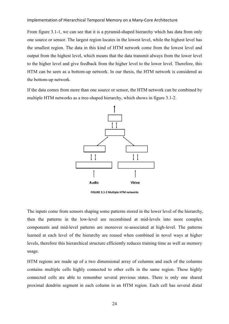
If the data comes from more than one source or sensor, the HTM network can be combined by
multiple HTM networks as a tree-shaped hierarchy, which shows in figure 3.1-2.
FIGURE 3.1-2 Multiple HTM networks
The inputs come from sensors shaping some patterns stored in the lower level of the hierarchy,
then the patterns in the low-level are recombined at mid-levels into more complex
components and mid-level patterns are moreover re-associated at high-level. The patterns
learned at each level of the hierarchy are reused when combined in novel ways at higher
levels, therefore this hierarchical structure efficiently reduces training time as well as memory
usage.
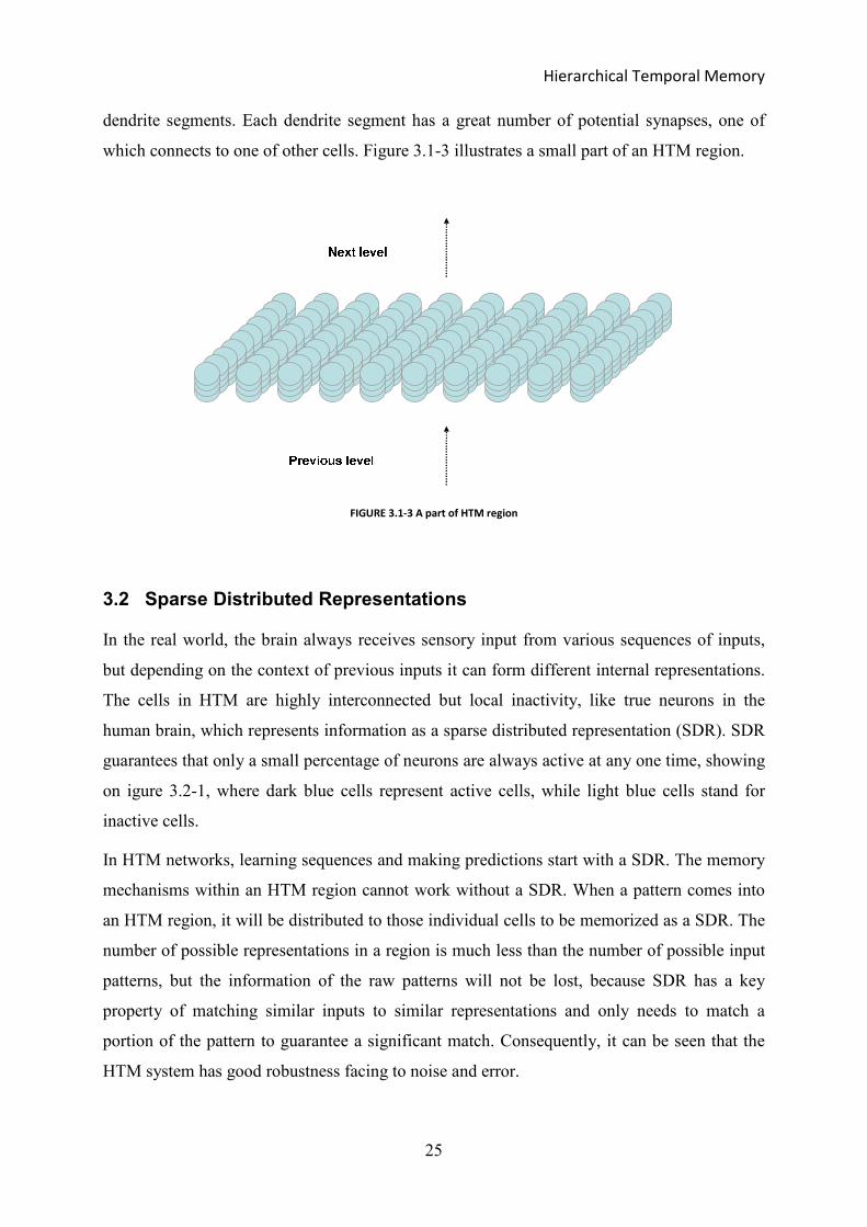
HTM regions are made up of a two dimensional array of columns and each of the columns
contains multiple cells highly connected to other cells in the same region. These highly
connected cells are able to remember several previous states. There is only one shared
proximal dendrite segment in each column in an HTM region. Each cell has several distal
Hierarchical Temporal Memory
25
dendrite segments. Each dendrite segment has a great number of potential synapses, one of
which connects to one of other cells. Figure 3.1-3 illustrates a small part of an HTM region.
FIGURE 3.1-3 A part of HTM region
3.2 Sparse Distributed Representations
In the real world, the brain always receives sensory input from various sequences of inputs,
but depending on the context of previous inputs it can form different internal representations.
The cells in HTM are highly interconnected but local inactivity, like true neurons in the
human brain, which represents information as a sparse distributed representation (SDR). SDR
guarantees that only a small percentage of neurons are always active at any one time, showing
on igure 3.2-1, where dark blue cells represent active cells, while light blue cells stand for
inactive cells.
In HTM networks, learning sequences and making predictions start with a SDR. The memory
mechanisms within an HTM region cannot work without a SDR. When a pattern comes into
an HTM region, it will be distributed to those individual cells to be memorized as a SDR. The
number of possible representations in a region is much less than the number of possible input
patterns, but the information of the raw patterns will not be lost, because SDR has a key
property of matching similar inputs to similar representations and only needs to match a
portion of the pattern to guarantee a significant match. Consequently, it can be seen that the
HTM system has good robustness facing to noise and error.

Implementation of Hierarchical Temporal Memory on a Many-Core Architecture
26
FIGURE 3.2-1 Sparse Distributed Representation
3.3 Core Functions of HTM
HTM has three intimately integrated core functions of every region: learning, inference and
prediction. Most pattern recognition algorithms are only able to identify some static patterns
recognition, but HTM algorithm is able to learn the spatial and temporal sequences from a
continuous stream of input data.
3.3.1 Learning
Brains can learn all the time and HTM tries to model this property by using an "on-line
learning" principle for its region. This on-line learning is important as it can continually learn
from each new input while doing inference. Each HTM region looks for spatial patterns then
learns temporal patterns. Spatial patterns are the combinations of inputs that occur together
often, while temporal patterns mean the sequence of those spatial patterns. Learning in an
HTM region could also be interpreted as sequence memory. The complexity of spatial
patterns learned by a region depends on how much memory is allocated to this region. The
more allocated memory, the more complex spatial patterns learned by a region.
3.3.2 Inference
The received inputs of an HTM will be matched to previous learned spatial and temporal
patterns. If the new inputs can be successfully matched to previously stored sequences, the
inference and pattern matching will be operated more accurately. However, many novel inputs

Hierarchical Temporal Memory
27
of HTMs are probably similar, like human brain always is facing, but the inputs may never
repeated precisely. SDR effectively copes with this kind of problem by matching only a
portion of patterns with the stored sequences.
3.3.3 Prediction
In an HTM region, prediction and inference are almost the same thing. In HTM, prediction is
formed in a region by matching current input with stored sequences of pattern, in order to
predict what possible inputs will follow. Predictions are continuous and context-sensitive,
because an HTM region will make different predictions, constantly based on different
contexts. Predictions are based on what has happened in the past and what is happening now.
3.4 HTM’s Learning and Prediction
Each HTM region looks for spatial patterns then learns temporal patterns. After learning, each
region makes predictions depending on its memory of sequences.
Each HTM region forms a sparse distributed representation of the input at first when a new
input comes, which is called “spatial pooler”. It then forms a representation of the input in the
context of previous inputs by activation a subset of the cells within each active column,
representatively only one cell will be activated per column. The final step for an HTM region
is to form a prediction based on the input in the context of previous inputs. These latter two
steps are referred to as the “temporal pooler”.
The term "spatial pooler" works on the shared proximal dendrite segment, at the level of
columns, to learn connections between input bits and columns. The "temporal pooler", which
operates on distal dendrite segments, at the level of cells, to learn feed-forward connections
between cells in the same region.
In HTM, for both the “spatial pooler” and the “temporal pooler”, terms such as cells, synapses,
potential synapses, dendrite segments, and columns are used throughout. HTM cells receive
feed-forward input coming from sensory data or from another region lower in the hierarchy
via the proximal dendrite segment, shown in figure 3.4-1. Each column of cells in HTM has
only one single shared proximal dendrite in order to respond to similar feed-forward input,
and each proximal dendrite has an associated set of potential synapses. HTM also has lateral
inputs from nearby cells through distal dendrites, illustrated in figure 3.4-2.

Implementation of Hierarchical Temporal Memory on a Many-Core Architecture
28
The "potential synapses" means there is a possibility to form a synapse between two dendrite
segments of two cells which are in different columns and it has a scalar permanence value
ranging from 0.0 to 1.0 which is adjusted during learning. When the permanence value is
above a threshold, the potential synapse will become a functional synapse, or we can say that
a synapse is established and the binary weight of such synapses is marked "1". A column will
become active if the number of its valid synapses which connected to active inputs is above a
threshold. In HTMs, learning involves increasing or decreasing the permanence values of all
potential synapses on a dendrite segment. The connectedness of a synapse will rely on how
large the permanence value is, thus the higher permanence is and the more difficult it will be
to disconnect the synapse. When the permanence value is below a threshold, the synapse has
no effect. In an HTM cell, the number of valid synapses on the proximal and distal dendrite
segments is not always constant, but the number of potential synapses is fixed.
3.4.1 Spatial Pooler Function
The spatial pooler function could be separated into three phases:
It firstly learns the connections to each column from a subset of the inputs and determines
how many established synapses on each column are connected to active inputs. Then the
number of active synapses is multiplied by a “boosting” factor. The columns with the
strongest activation after boosting inhibit other columns in the neighborhood of the active
ones with a weaker activation. The third phase is to update the permanence values of all the
potential synapses for learning. The permanence values of synapses connected to active inputs
will be increased, while the permanence values of synapses connected to inactive inputs will
be decreased (Hebbian rule [20]).
A new input leads to a sparse set of active columns. Different input patterns cause different
levels of activation of the columns. These three phases sufficiently reflect in the sparse
distributed representation, which is the fundamental function of the spatial pooler, and to be
the input for the temporal learning phase at the same level.

Hierarchical Temporal Memory
29
FIGURE 3.4-1 One column in an HTM region
In figure 3.4-1, four cells comprising a column which share a common proximal dendrite
segment which has a set of potential synapses representing a subset of the inputs. Ten round
spots stand for potential synapses. Solid spots represent valid synapses. These valid synapses
have their permanence value exceed the connection threshold due to their connection to active
inputs. White spots represent non-valid synapses, because each permanence value of them is
lower than the threshold. The column is inactivity before activated. When the number of valid
synapses is above a threshold, the column will be activated by the feed-forward input.
3.4.2 Temporal Pooler Function
The temporal pooler function can also be separated into three phases:
It firstly calculates the active state for each cell that is in a winning column (the columns
which inhibit others are called winning columns). Then it computes the predictive state for
each cell. In the third phase the synapses will be updated to enable learning. Phase 1 and
phase 2 are performed while a network is learning as well as during inference. Phase 3 is
performed during learning only.

Implementation of Hierarchical Temporal Memory on a Many-Core Architecture
30
Phase 1: cells activated by feed-forward input become activate
Each cell in the HTM region has several distal dendrite segments, each of which has many
potential synapses connecting to cells of other columns. For each active column which is
activated by feed-forward input, if any of its cells are already in a predictive state from a
previous time step, only those cells will be activated. A cell which is in a predictive state
means that the current activation was expected, the cell then becomes active from the
predictive state and is chosen as the learning cell. If the input was not predicted, all cells in the
column will become active when the column is activated, because without context usually
cannot predict what is likely to happen next and all options are possible. Moreover, the cell
which has the best matching dendrite segment (the best matching dendrite segment is the
segment which has the largest number of active synapses) is chosen as the learning cell. The
resulting set of activated cells is the representation of the current input in the context of
previous input.
Identical inputs always lead to the same number of columns in the same position to be active,
but a different combination of cells would be activated among those columns in the different
context of previous inputs.
Phase 2: cells activated by lateral input enter predictive state
For every dendrite segment on every cell in the region, if the number of its established
synapses which connect to current active cells exceeds a threshold, then this dendrite segment
is seen as active and the cell which possesses the active dendrite segment enters a predictive
state unless it already activated due to feed-forward input. When a dendrite segment is marked
as active, the permanence values of all synapses associated with this segment are modified.
For every potential synapse on the active dendrite segment, the permanence values of
synapses connected to active cells will be increased, while the permanence values of synapses
connected to inactive cells will be decreased, which are marked as ‘temporary’.
In addition to modifying the permanence values of the synapses connected with the active
segment, a second segment is chosen for extending predictions further back in time. The
second segment is the cell’s segment that best matches the state of the system in the previous
time step. For the segment, increment the permanence values of synapses that are connected
to active cells, while the permanence values of synapses connected to inactive cells will be
decremented. These modifications are also marked as ‘temporary’.
Hierarchical Temporal Memory
31
Whenever a cell from being inactive becomes active due to feed-forward input, we remove
any temporary marks. If the cell correctly predicted the feed-forward input, the permanence of
synapses of this cell could be updated.
Phase 3: update synapses for learning
If a column has a cell in learning state, the queued segment updates are positively reinforced.
If a column had a cell in predictive state at the previous time step, but not in predictive state at
this time step, which means the cell stops prediction for any reason, the queued segment
updates will be negatively reinforced.
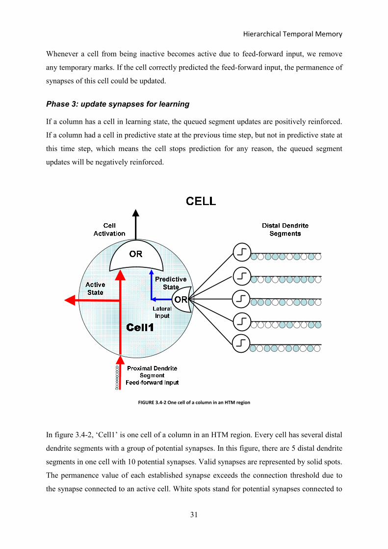
FIGURE 3.4-2 One cell of a column in an HTM region
In figure 3.4-2, ‘Cell1’ is one cell of a column in an HTM region. Every cell has several distal
dendrite segments with a group of potential synapses. In this figure, there are 5 distal dendrite
segments in one cell with 10 potential synapses. Valid synapses are represented by solid spots.
The permanence value of each established synapse exceeds the connection threshold due to
the synapse connected to an active cell. White spots stand for potential synapses connected to

Implementation of Hierarchical Temporal Memory on a Many-Core Architecture
32
inactive cells with their permanence value lower than threshold. The column in which the
‘Cell1’ is located becomes activated due to feed-forward input through the proximal dendrite
segment, which is shown in the red coarse arrow in the bottom-left. The ‘Cell1’ may enter its
predictive state as long as at least one of its dendrite segments is connected to enough active
cells within its learning radius (learning radius is a certain range around the cell except the
other cells in the same column to which it belongs), which is shown in the blue thin arrow in
the right. A cell’s state of predictive or non-predictive only makes contribution to the feed-
forward output of a cell and is not propagated laterally.
The output of a region is the logical OR of the state of all cells, including the cells’ active
state because of feed-forward input and the cells’ predictive state by lateral input.
Adapteva Epiphany
33
4 Adapteva Epiphany
Adapteva Epiphany is the given hardware used for our implementation of the HTM algorithm.
This chapter will introduce the EpiphanyTM
many-core architecture which is developed by
Adapteva [11, 18, 19].
The EpiphanyTM
architecture is a scalable many-core architecture using a shared-memory
model. It is able to deal with parallel computing problems like image processing,
communication, sensor signal processing, encryption and compression. It has many cores on a
single chip interconnected by eMesh network which makes power reduction compared with a
traditional crossbar interconnection. It has a good scalability which reflects in that the number
of cores is able to extend to as many as 4096 individual cores on a single chip.
4.1 Introduction of Epiphany
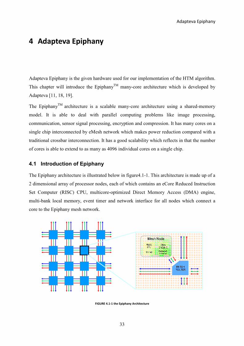
The Epiphany architecture is illustrated below in figure4.1-1. This architecture is made up of a
2 dimensional array of processor nodes, each of which contains an eCore Reduced Instruction
Set Computer (RISC) CPU, multicore-optimized Direct Memory Access (DMA) engine,
multi-bank local memory, event timer and network interface for all nodes which connect a
core to the Epiphany mesh network.
FIGURE 4.1-1 the Epiphany Architecture
Implementation of Hierarchical Temporal Memory on a Many-Core Architecture
34
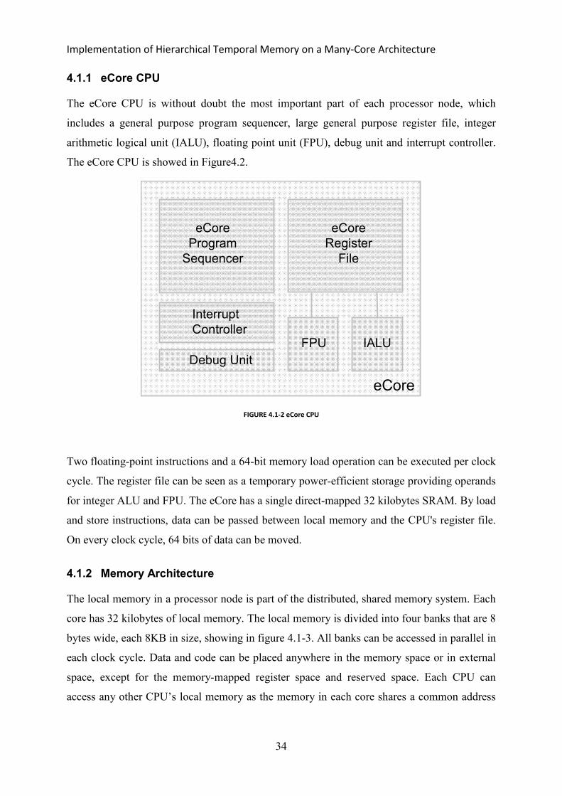
4.1.1 eCore CPU
The eCore CPU is without doubt the most important part of each processor node, which
includes a general purpose program sequencer, large general purpose register file, integer
arithmetic logical unit (IALU), floating point unit (FPU), debug unit and interrupt controller.
The eCore CPU is showed in Figure4.2.
eCore
Program
Sequencer
eCore
Register
File
Interrupt
ControllerFPU IALU
Debug Unit
eCore
FIGURE 4.1-2 eCore CPU
Two floating-point instructions and a 64-bit memory load operation can be executed per clock
cycle. The register file can be seen as a temporary power-efficient storage providing operands
for integer ALU and FPU. The eCore has a single direct-mapped 32 kilobytes SRAM. By load
and store instructions, data can be passed between local memory and the CPU's register file.
On every clock cycle, 64 bits of data can be moved.
4.1.2 Memory Architecture
The local memory in a processor node is part of the distributed, shared memory system. Each
core has 32 kilobytes of local memory. The local memory is divided into four banks that are 8
bytes wide, each 8KB in size, showing in figure 4.1-3. All banks can be accessed in parallel in
each clock cycle. Data and code can be placed anywhere in the memory space or in external
space, except for the memory-mapped register space and reserved space. Each CPU can
access any other CPU’s local memory as the memory in each core shares a common address
Adapteva Epiphany
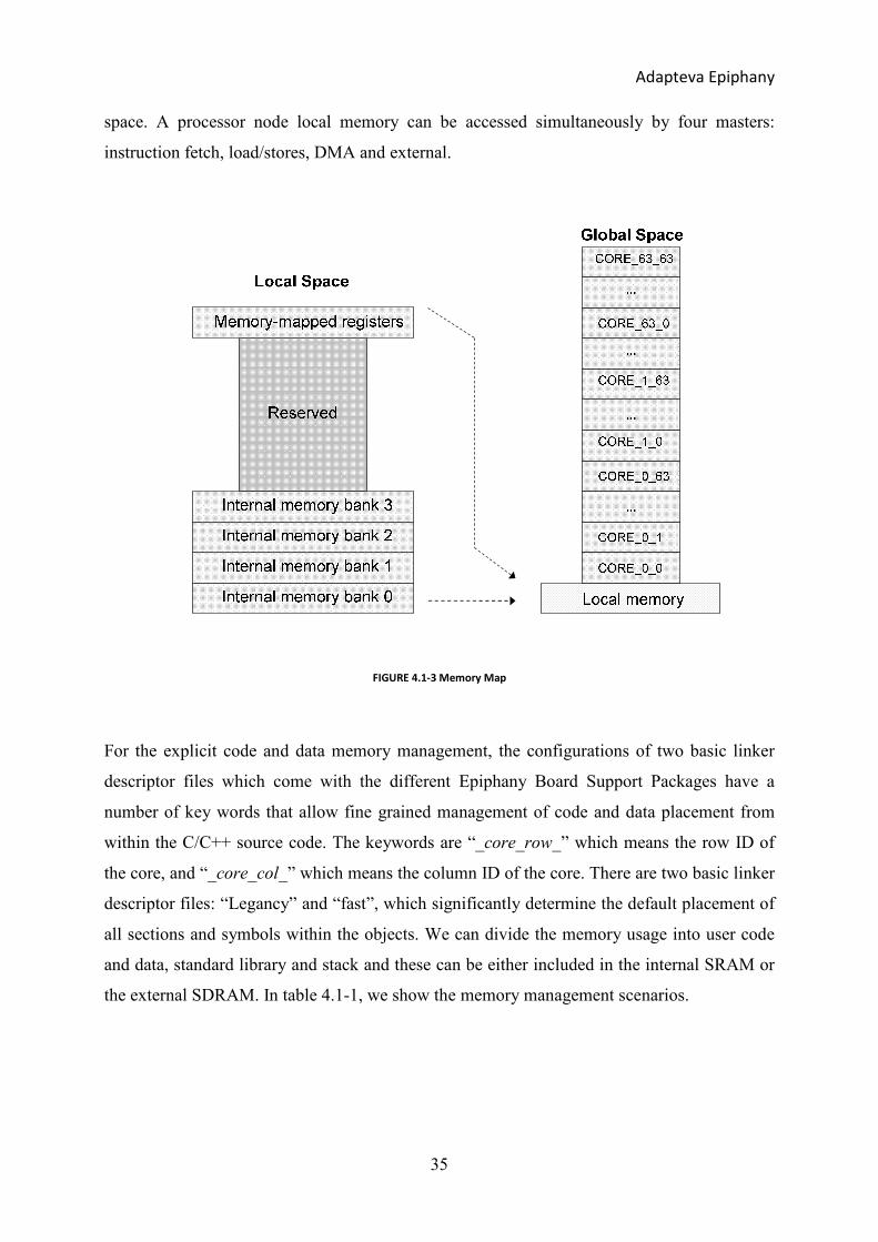
35
space. A processor node local memory can be accessed simultaneously by four masters:
instruction fetch, load/stores, DMA and external.
FIGURE 4.1-3 Memory Map
For the explicit code and data memory management, the configurations of two basic linker
descriptor files which come with the different Epiphany Board Support Packages have a
number of key words that allow fine grained management of code and data placement from
within the C/C++ source code. The keywords are “_core_row_” which means the row ID of
the core, and “_core_col_” which means the column ID of the core. There are two basic linker
descriptor files: “Legancy” and “fast”, which significantly determine the default placement of
all sections and symbols within the objects. We can divide the memory usage into user code
and data, standard library and stack and these can be either included in the internal SRAM or
the external SDRAM. In table 4.1-1, we show the memory management scenarios.

Implementation of Hierarchical Temporal Memory on a Many-Core Architecture
36
TABLE 4.1-1 Memory management scenarios
4.1.3 2D eMesh Network
This eMesh network is 2-dimensional network, which makes high speed inter-processor
communication possible. A mesh node router is connected to the four nearest-neighbors.
Every core can transfer up to 8 bytes of data in every cycle between its CPU and router. Three
individual mesh structures serving different types of transaction traffic comprise the eMesh
Network-On-Chip (NOC), cMesh, rMesh, and xMesh and they are orthogonal, which is
shown in Figure 4.1-3.
File
USER
CODE &
DATA
STANDARD
LIBRARY STACK NOTE
legacy.ldf External
SDRAM
External
SDRAM
External
SDRAM
Use to run any legacy code with up to 1MB of
combined code and data.
fast.ldf Internal
SRAM
External
SDRAM
Internal
SRAM
Places all user code and static data in local memory,
including the stack. Use to implement fast critical
functions. It is the user’s responsibility to ensure
that the code fits within the local memory.
internal.ldf Internal
SRAM
Internal
SRAM
Internal
SRAM
Places all code and static data in local memory,
including the stack. Use to implement fastest
applications. It is the user’s responsibility to ensure
that the code fits within the local memory.

Adapteva Epiphany
37
Mesh Node
RISC
CPU
DMA
ENGINE
MemoryNetwork
Interface
EMESH
ROUTER
Mesh Node
RISC
CPU
DMA
ENGINE
MemoryNetwork
Interface
EMESH
ROUTER
Mesh Node
RISC
CPU
DMA
ENGINE
MemoryNetwork
Interface
EMESH
ROUTER
Mesh Node
RISC
CPU
DMA
ENGINE
MemoryNetwork
Interface
EMESH
ROUTER
On-chip write Network
Off-chip write Network
Read request Network
FIGURE 4.1-4 eMesh Network
4.1.4 Direct Memory Access
Each Epiphany mesh node includes a DMA engine which enables accelerated data movement
between eMesh nodes within the chip. Information can be prefetched autonomously by a
DMA engine, while the DMA engine is configured under software control. The clock speed of
DMA is the same as for the cores.
4.1.5 Event Timers
There are two 32-bit event timers which can operate independently to monitor key events
within the processor node in each processor node. A distributed set of event timers are
supported by the Epiphany architecture. The timers can be used for program debug, program
optimization, load balancing, traffic balancing, timeout counting, watchdog timing, system
time and numerous other purposes.

Implementation of Hierarchical Temporal Memory on a Many-Core Architecture
38
4.2 Mapping on the Epiphany
The Adapteva Epiphany fabric is integrated to an evaluation board named anemone104
developed by BittWare, which is connected to an Altera Stratix III FPGA development board.
The Altera Stratix III FPGA also provides a 32 megabyte external memory to the AN104 and
a USB 2.0 interface for accessing the AN104.
For this project, the integrated development environment (IDE) Eclipse was used to develop,
debug and download code to the Epiphany fabric. It is easy to create, manage and navigate C
based many-core projects as well as compiling, linking and debugging by using
Eclipse.
The Epiphany Software Development Kit (ESDK) enables out-of-the-box execution of
applications written in regular ANSI-C and does not require any C-subset, language
extensions, or SIMD style programming. The ESDK includes optimized ANSI-C compiler,
robust multicore Eclipse IDE (based on Indigo), multicore debugger (based on gdb-7.3),
multicore communication and hardware utility libraries and a fast functional simulator with
instruction trace capability. An Epiphany complier is based on the popular GNU GCC, which
supports a wide range of options, allowing for a fine tuning of the compilation process. The
Epiphany assembler ‘e-as’, parses a file of assembly code to produce an object file for use by
the linker ‘e-ld’. A set of libraries based on the newlib distribution of Standard C and
Standard Math libraries for embedded systems are included in the ESDK, which are bundled
with the ‘e-gcc’ complier. The Epiphany Hardware Utility library (eLib) also included in the
ESDK, provides functions for configuring and querying the Epiphany hardware resources.
The Epiphany debugger (e-gdb) based on the popular GNU GDB is used to debug the many-
core project, which allows a programmer to see what is going on inside a program while it
executes. The E-GDB includes some powerful debug features, such as: interactive program
load, stopping program on specific conditions, examine complete state of machine and
program once program has stopped and continuing program one instruction at a time or until
the nest stop condition is met. However, the epiphany implementation of GDB currently lacks
support for tracing and hardware assisted watchpoints. And it starts on debug session for each
core which for 16 cores somewhat is manageable, but for hundreds of processors will be
unmanageable.

Implementation
39
5 Implementation
This thesis aims at evaluating the performance of mapping the HTM algorithm onto the
Adapteva Epiphany many-core architecture by programming in C.
This chapter will describe the implementation procedure of the whole work. Section 5.1
describes the HTM network we used in this thesis work. For the pattern recognition tasks,
training sets are of the essence and described in section 5.2. The HTM algorithm will be
mapped onto a many-core architecture, first a sequential implementation described in section
5.3. Then in 5.4 we describe some alternative mapping methods and give a detailed
description of the three selected mapping methods. Finally, section 5.5 describes how the
HTM algorithm simulated in OpenMP.
5.1 HTM Algorithm Programming
HTM is a relatively sophisticated machine learning algorithm and it is nontrivial to implement
on the parallel computer. The first step for implementing HTM on the proposed many-core
architecture is to program HTM in C. In this project, a region in HTM is made up of 16 by 16
columns, each of which contains 4 cells, because the size of training images is 16*16 pixels,
illustrated in Figure 5.1-1. An ideally complete HTM network is a hierarchical construction
with a certain number of levels, while only a one level HTM network has been implemented
in this project. Because our training examples are not that complex, the one level HTM
network is enough to process them.
FIGURE 5.1-1 A one-level HTM Network with 16 by 16 columns
Implementation of Hierarchical Temporal Memory on a Many-Core Architecture
40
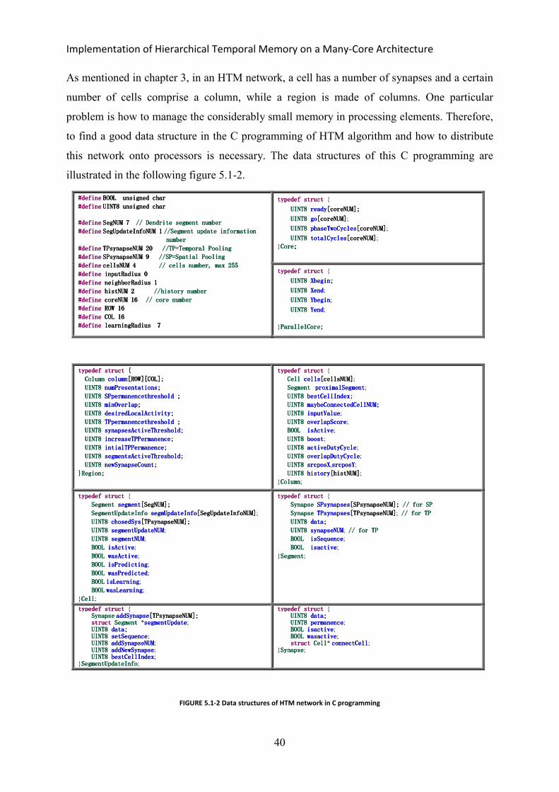
As mentioned in chapter 3, in an HTM network, a cell has a number of synapses and a certain
number of cells comprise a column, while a region is made of columns. One particular
problem is how to manage the considerably small memory in processing elements. Therefore,
to find a good data structure in the C programming of HTM algorithm and how to distribute
this network onto processors is necessary. The data structures of this C programming are
illustrated in the following figure 5.1-2.
#define#define#define#define BOOL unsigned char BOOL unsigned char BOOL unsigned char BOOL unsigned char
#define#define#define#define UINT8 unsigned char UINT8 unsigned char UINT8 unsigned char UINT8 unsigned char
#define#define#define#define SegNUM 7 SegNUM 7 SegNUM 7 SegNUM 7 // Dendrite segment number// Dendrite segment number// Dendrite segment number// Dendrite segment number
#define#define#define#define SegUpdateInfoNUM 1SegUpdateInfoNUM 1SegUpdateInfoNUM 1SegUpdateInfoNUM 1 //Segment update information//Segment update information//Segment update information//Segment update information
numbernumbernumbernumber
#define#define#define#define TPsynapseNUM 20 TPsynapseNUM 20 TPsynapseNUM 20 TPsynapseNUM 20 //TP=Temporal Pooling//TP=Temporal Pooling//TP=Temporal Pooling//TP=Temporal Pooling
#define#define#define#define SPsynapseNUM 9 SPsynapseNUM 9 SPsynapseNUM 9 SPsynapseNUM 9 //SP=Spatial Pooling//SP=Spatial Pooling//SP=Spatial Pooling//SP=Spatial Pooling
#define#define#define#define cellsNUM 4cellsNUM 4cellsNUM 4cellsNUM 4 // cells number, max 255// cells number, max 255// cells number, max 255// cells number, max 255
#define #define #define #define inputRadius 0 inputRadius 0 inputRadius 0 inputRadius 0
#define#define#define#define neighborRadius 1neighborRadius 1neighborRadius 1neighborRadius 1
#define#define#define#define histNUM 2 histNUM 2 histNUM 2 histNUM 2 //history number//history number//history number//history number
#define#define#define#define coreNUM 16 coreNUM 16 coreNUM 16 coreNUM 16 // core number// core number// core number// core number
#define #define #define #define ROW 16ROW 16ROW 16ROW 16
#define #define #define #define COL 16COL 16COL 16COL 16
#define #define #define #define learningRadius learningRadius learningRadius learningRadius 7777
typedef struct typedef struct typedef struct typedef struct {
UINT8 UINT8 UINT8 UINT8 readyreadyreadyready[coreNUM];[coreNUM];[coreNUM];[coreNUM];
UINT8 UINT8 UINT8 UINT8 gogogogo[coreNUM][coreNUM][coreNUM][coreNUM];
UINT8 UINT8 UINT8 UINT8 phaseTwoCyclesphaseTwoCyclesphaseTwoCyclesphaseTwoCycles[coreNUM][coreNUM][coreNUM][coreNUM];
UINT8 UINT8 UINT8 UINT8 totalCyclestotalCyclestotalCyclestotalCycles[coreNUM][coreNUM][coreNUM][coreNUM];
}CoreCoreCoreCore;;;;
typedef struct typedef struct typedef struct typedef struct {
UINT8 UINT8 UINT8 UINT8 XbeginXbeginXbeginXbegin;;;;
UINT8 UINT8 UINT8 UINT8 XendXendXendXend;
UINT8 UINT8 UINT8 UINT8 YbeginYbeginYbeginYbegin;
UIUIUIUINT8 NT8 NT8 NT8 YendYendYendYend;
}ParallelCoreParallelCoreParallelCoreParallelCore;;;;
typedef struct typedef struct typedef struct typedef struct {{{{
Column Column Column Column columncolumncolumncolumn[ROW][COL][ROW][COL][ROW][COL][ROW][COL];;;;
UINT8UINT8UINT8UINT8 numPresentationsnumPresentationsnumPresentationsnumPresentations;;;;
UINT8UINT8UINT8UINT8 SPpermanencethreshold SPpermanencethreshold SPpermanencethreshold SPpermanencethreshold ;;;;
UINT8UINT8UINT8UINT8 minOverlapminOverlapminOverlapminOverlap;;;;
UINT8UINT8UINT8UINT8 desiredLocalActivitydesiredLocalActivitydesiredLocalActivitydesiredLocalActivity;;;;
UINT8 UINT8 UINT8 UINT8 TPpermanencethreshold TPpermanencethreshold TPpermanencethreshold TPpermanencethreshold ;;;;
UINT8 UINT8 UINT8 UINT8 synapsesActiveThresholdsynapsesActiveThresholdsynapsesActiveThresholdsynapsesActiveThreshold;;;;
UINT8UINT8UINT8UINT8 increaseincreaseincreaseincreaseTPTPTPTPPermanencePermanencePermanencePermanence;;;;
UINT8 UINT8 UINT8 UINT8 iiiintialTPntialTPntialTPntialTPPermanencePermanencePermanencePermanence;;;;
UINT8 UINT8 UINT8 UINT8 segmentsActiveThresholdsegmentsActiveThresholdsegmentsActiveThresholdsegmentsActiveThreshold;;;;
UINT8 UINT8 UINT8 UINT8 newSynapseCountnewSynapseCountnewSynapseCountnewSynapseCount;;;;
}}}}RRRRegionegionegionegion;;;;
typedef struct typedef struct typedef struct typedef struct {
Cell Cell Cell Cell cellscellscellscells[cellsNUM][cellsNUM][cellsNUM][cellsNUM];
Segment Segment Segment Segment proximalSegmentproximalSegmentproximalSegmentproximalSegment;
UINT8 UINT8 UINT8 UINT8 bestCellIndex;bestCellIndex;bestCellIndex;bestCellIndex;
UINT8 UINT8 UINT8 UINT8 maybeConnectedCellNUM;maybeConnectedCellNUM;maybeConnectedCellNUM;maybeConnectedCellNUM;
UINT8 UINT8 UINT8 UINT8 inputValueinputValueinputValueinputValue;
UINT8 UINT8 UINT8 UINT8 overlapScoreoverlapScoreoverlapScoreoverlapScore;
BOOL BOOL BOOL BOOL isActiveisActiveisActiveisActive;
UINT8 UINT8 UINT8 UINT8 boostboostboostboost;
UINT8 UINT8 UINT8 UINT8 activeDutyCycleactiveDutyCycleactiveDutyCycleactiveDutyCycle;
UINT8 UINT8 UINT8 UINT8 overlapDutyCycleoverlapDutyCycleoverlapDutyCycleoverlapDutyCycle;
UINT8 UINT8 UINT8 UINT8 srcposXsrcposXsrcposXsrcposX,srcposYsrcposYsrcposYsrcposY;
UINT8 UINT8 UINT8 UINT8 historyhistoryhistoryhistory[histNUM][histNUM][histNUM][histNUM];
}ColumnColumnColumnColumn;
typedef struct typedef struct typedef struct typedef struct {
SegmentSegmentSegmentSegment segsegsegsegmentmentmentment[SegNUM];[SegNUM];[SegNUM];[SegNUM];
SegmentUpdateInfo SegmentUpdateInfo SegmentUpdateInfo SegmentUpdateInfo segmUpdateInfosegmUpdateInfosegmUpdateInfosegmUpdateInfo[SegUpdateInfoNUM][SegUpdateInfoNUM][SegUpdateInfoNUM][SegUpdateInfoNUM];
UINT8 UINT8 UINT8 UINT8 chosedSyschosedSyschosedSyschosedSys[TPsynapseNUM][TPsynapseNUM][TPsynapseNUM][TPsynapseNUM];;;;
UINT8 UINT8 UINT8 UINT8 segmentUpdateNUMsegmentUpdateNUMsegmentUpdateNUMsegmentUpdateNUM;
UINT8 UINT8 UINT8 UINT8 segmentNUMsegmentNUMsegmentNUMsegmentNUM;
BOOL BOOL BOOL BOOL isActiveisActiveisActiveisActive;
BOOL BOOL BOOL BOOL wasActivewasActivewasActivewasActive;
BOOLBOOLBOOLBOOL isPredictingisPredictingisPredictingisPredicting;
BOOBOOBOOBOOLLLL wasPredictedwasPredictedwasPredictedwasPredicted;
BOOLBOOLBOOLBOOL isLearningisLearningisLearningisLearning;
BOOLBOOLBOOLBOOL wasLearningwasLearningwasLearningwasLearning;
}CellCellCellCell;
typedef struct typedef struct typedef struct typedef struct {
SynapseSynapseSynapseSynapse SPsynapsesSPsynapsesSPsynapsesSPsynapses[SPsynapseNUM]; [SPsynapseNUM]; [SPsynapseNUM]; [SPsynapseNUM]; // for SP// for SP// for SP// for SP
SynapseSynapseSynapseSynapse TPsynapsesTPsynapsesTPsynapsesTPsynapses[TPsynapseNUM][TPsynapseNUM][TPsynapseNUM][TPsynapseNUM]; // for TP// for TP// for TP// for TP
UINT8 UINT8 UINT8 UINT8 datadatadatadata;;;;
UINT8 UINT8 UINT8 UINT8 synapseNUMsynapseNUMsynapseNUMsynapseNUM; // for TP// for TP// for TP// for TP
BOOLBOOLBOOLBOOL isSequenceisSequenceisSequenceisSequence;
BOOLBOOLBOOLBOOL isactiveisactiveisactiveisactive;
}SegmentSegmentSegmentSegment;
typedef struct typedef struct typedef struct typedef struct { SynapseSynapseSynapseSynapse addSynapseaddSynapseaddSynapseaddSynapse[TPsynapseNUM];[TPsynapseNUM];[TPsynapseNUM];[TPsynapseNUM]; struct struct struct struct Segment Segment Segment Segment *segmentUpdatesegmentUpdatesegmentUpdatesegmentUpdate; UINT8 UINT8 UINT8 UINT8 datadatadatadata;;;;
UINT8 UINT8 UINT8 UINT8 setSequencesetSequencesetSequencesetSequence; UINT8 UINT8 UINT8 UINT8 addSynapseNUMaddSynapseNUMaddSynapseNUMaddSynapseNUM; UINT8 UINT8 UINT8 UINT8 addNewSynapseaddNewSynapseaddNewSynapseaddNewSynapse; UINT8 UINT8 UINT8 UINT8 bestCellIndexbestCellIndexbestCellIndexbestCellIndex;
}SegmentUpdateInfoSegmentUpdateInfoSegmentUpdateInfoSegmentUpdateInfo;
typedef struct typedef struct typedef struct typedef struct { UINT8 UINT8 UINT8 UINT8 datadatadatadata;;;;
UINT8 UINT8 UINT8 UINT8 permanencepermanencepermanencepermanence; BOOL BOOL BOOL BOOL isactiveisactiveisactiveisactive; BOOL BOOL BOOL BOOL wasactivewasactivewasactivewasactive; struct struct struct struct CellCellCellCell* connectCellconnectCellconnectCellconnectCell;
}SynapseSynapseSynapseSynapse;
FIGURE 5.1-2 Data structures of HTM network in C programming

Implementation
41
Here, isactive, wasactive, isprediction, waspredicted, islearning, waslearning are all Boolean
value, using ‘char’ type is better than ‘int’ type to save the memory. From figure 5.1-2, the
certain number of segments, segment update information, temporal pooling synapses, spatial
pooling synapses, cells, input radius, neighbor radius, history, core, row, column as well as
learning radius is defined. In our task, each cell has set 7 distal dendrite segments, each of
which has 20 synapses. The “neighborRadius” and the ‘learningRadius’ both mean a certain
range around the cell except the other cells in the same column to which it belongs, but they
are set to a different range. The neighbor radius is set to 1, while the learning radius is set to 7.
From figure 5.1-2 we can see that the structure ‘Region’ is the outermost layer, which nests
several layers of structures. Therefore, it occupies a relatively large amount of memory space,
4.2MB. The memory usage of each structure illustrates in figure 5.1-3.
32 M
32 M
32 M
32 M
B M
emor
yB
Mem
ory
B M
emor
yB
Mem
ory
Structure Memory usage
CoreCoreCoreCore core 256 Bytes
ParallelCoreParallelCoreParallelCoreParallelCore coreID[coreNUM] 16 Bytes
UINT8UINT8UINT8UINT8 inputData[ROW][COL] 1024 Bytes
UINT8UINT8UINT8UINT8 steps[stepNUM] 64 Bytes
RegionRegionRegionRegion region 4.2 Megabytes
UINT8UINT8UINT8UINT8 testOut[ROW][COL] 1024 Bytes
FIGURE 5.1-3 Memory map
There exist a lot of ‘for’ loops in some important functions in the HTM’s implementation.
These ‘for’ loops are a very good target for parallelization, because the block of code will
contain a lot of repeated calculations and significant execution time [18]. Some typical ‘for’
loops will be described in section 5.1.1 and 5.1.2.

Implementation of Hierarchical Temporal Memory on a Many-Core Architecture
42
5.1.1 Spatial Pooling Implementation
The spatial pooling function used to process at the level of columns. In this function, some
columns will be activated by active input through feed-forward input, which shows in figure
5.1-4 and active columns are marked in blue. This function is divided into three distinct
phases in our C implementation. Phase1 computes the overlap of all columns, and phase2
computes the winning columns after local inhibition, furthermore, phase3 increases of
decreases synapse permanence and internal variables.
FIGURE 5.1-4 Spatial pooling implementation
1 for ( int i=columnRowStart;i<columnRowEnd;i++)
2 for ( int j=columnColStart;j<columnColEnd;j++) // main part suits for parallel implementation// main part suits for parallel implementation// main part suits for parallel implementation// main part suits for parallel implementation
3 for ( int x=minX; x<=maxX; x++) // minX, maxX mean neighbor radiusminX, maxX mean neighbor radiusminX, maxX mean neighbor radiusminX, maxX mean neighbor radius
4 for ( int y=minY; y<=maxY; y++)
5 If (region.column[x][y].overlapScore> region.column[i][j].overlapScore)
FIGURE 5.1-5 Pseudo code used in each phase in Spatial polling implementation

Implementation
43
When parallel in columns level, showing in figure 5.1-5, ‘i’ and ‘j’ are the coordinate of a
column. Here ‘i’ is iterating along the row dimension, and ‘j’ is iterating along the column
dimension. Here ‘x’ and ‘y’ are coordinates within the neighbor radius of such column. Line 1
and 2 of these codes in figure 5.1-5 are the main part which are suitable to be parallel. The last
line of this code snippet is used to judge whether the column[x][y] is inhibited or not. These
pseudo codes are used in each phase of spatial pooling implementation respectively.
5.1.2 Temporal Pooling Implementation
As mentioned in chapter 3, temporal pooling algorithm focuses on operating at the level of
individual cells within columns. In this function, some cells within active columns will be
activated by feed-forward input or lateral input, which shows in figure 5.1-6 and active cells
are marked in dark blue. Cells activated by feed-forward input will become active, while cells
activated by lateral input will enter predictive state. If the input was not predicted, all cells in
the column will become active when the column is activated, because without context usually
cannot predict what is likely to happen next and all options are possible. Moreover, the cell
which has the best matching dendrite segment will be chosen as the learning cell.
FIGURE 5.1-6 Temporal pooling implementation
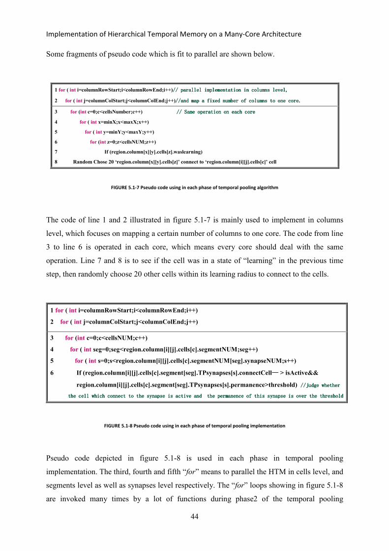
Implementation of Hierarchical Temporal Memory on a Many-Core Architecture
44
Some fragments of pseudo code which is fit to parallel are shown below.
1 for ( int i=columnRowStart;i<columnRowEnd;i++)// parallel implementation in columns level, // parallel implementation in columns level, // parallel implementation in columns level, // parallel implementation in columns level,
2 for ( int j=columnColStart;j<columnColEnd;j++)//and map a fixed number of columns to one core.//and map a fixed number of columns to one core.//and map a fixed number of columns to one core.//and map a fixed number of columns to one core.
3 for (int c=0;c<cellsNumber;c++) // Same operation on each core// Same operation on each core// Same operation on each core// Same operation on each core
4 for ( int x=minX;x<maxX;x++)
5 for ( int y=minY;y<maxY;y++)
6 for (int z=0;z<cellsNUM;z++)
7 If (region.column[x][y].cells[z].waslearning)
8 Random Chose 20 ‘region.column[x][y].cells[z]’ connect to ‘region.column[i][j].cells[c]’ cell
FIGURE 5.1-7 Pseudo code using in each phase of temporal pooling algorithm
The code of line 1 and 2 illustrated in figure 5.1-7 is mainly used to implement in columns
level, which focuses on mapping a certain number of columns to one core. The code from line
3 to line 6 is operated in each core, which means every core should deal with the same
operation. Line 7 and 8 is to see if the cell was in a state of “learning” in the previous time
step, then randomly choose 20 other cells within its learning radius to connect to the cells.
1 for ( int i=columnRowStart;i<columnRowEnd;i++)
2 for ( int j=columnColStart;j<columnColEnd;j++)
3 for (int c=0;c<cellsNUM;c++)
4 for ( int seg=0;seg<region.column[i][j].cells[c].segmentNUM;seg++)
5 for ( int s=0;s<region.column[i][j].cells[c].segmentNUM[seg].synapseNUM;s++)
6 If (region.column[i][j].cells[c].segment[seg].TPsynapses[s].connectCell———— > isActive&&
region.column[i][j].cells[c].segment[seg].TPsynapses[s].permanence>threshold) //judge whether//judge whether//judge whether//judge whether
the cell which connect to the synathe cell which connect to the synathe cell which connect to the synathe cell which connect to the synapse is active and the permanence of this synapse is over the thresholdpse is active and the permanence of this synapse is over the thresholdpse is active and the permanence of this synapse is over the thresholdpse is active and the permanence of this synapse is over the threshold
FIGURE 5.1-8 Pseudo code using in each phase of temporal pooling implementation
Pseudo code depicted in figure 5.1-8 is used in each phase in temporal pooling
implementation. The third, fourth and fifth “for” means to parallel the HTM in cells level, and
segments level as well as synapses level respectively. The “for” loops showing in figure 5.1-8
are invoked many times by a lot of functions during phase2 of the temporal pooling
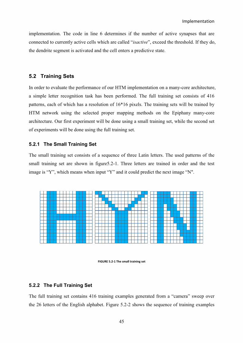
Implementation
45
implementation. The code in line 6 determines if the number of active synapses that are
connected to currently active cells which are called “isactive”, exceed the threshold. If they do,
the dendrite segment is activated and the cell enters a predictive state.
5.2 Training Sets
In order to evaluate the performance of our HTM implementation on a many-core architecture,
a simple letter recognition task has been performed. The full training set consists of 416
patterns, each of which has a resolution of 16*16 pixels. The training sets will be trained by
HTM network using the selected proper mapping methods on the Epiphany many-core
architecture. Our first experiment will be done using a small training set, while the second set
of experiments will be done using the full training set.
5.2.1 The Small Training Set
The small training set consists of a sequence of three Latin letters. The used patterns of the
small training set are shown in figure5.2-1. Three letters are trained in order and the test
image is “Y”, which means when input “Y” and it could predict the next image “N".
FIGURE 5.2-1 The small training set
5.2.2 The Full Training Set
The full training set contains 416 training examples generated from a “camera” sweep over
the 26 letters of the English alphabet. Figure 5.2-2 shows the sequence of training examples

Implementation of Hierarchical Temporal Memory on a Many-Core Architecture
46
sweeping from A to B. The 416 training examples will be used in the second experiment to be
trained 50 times, in total, 20800 iterations. In the test step, any one of training examples could
be input and the next one will be predicted.
FIGURE 5.2-2 The example of full training set
5.3 Single-core Implementation
This single-core implementation establishes a baseline for comparison with parallel
implementation to calculate the speedup and efficiency of parallel implementation. Since the
performance evaluation mainly focuses on speedup and efficiency, it is essential to record the
execution time of each mapping. Figure 5.3-1 gives the code of calculating clock cycles,
hence the execution time can be recorded according to the calculation.
void void void void init_timerinit_timerinit_timerinit_timer( )( )( )( )
{
int int int int start;start;start;start;
timerCountimerCountimerCountimerCount=0;t=0;t=0;t=0;
start = e_ctimer_startstart = e_ctimer_startstart = e_ctimer_startstart = e_ctimer_start (((( E_CTIMER_0, E_CTIMER_CLK E_CTIMER_0, E_CTIMER_CLK E_CTIMER_0, E_CTIMER_CLK E_CTIMER_0, E_CTIMER_CLK ))));
start = e_ctimer_set( start = e_ctimer_set( start = e_ctimer_set( start = e_ctimer_set( E_CTIMER_0, E_CTIMER_CLK,E_CTIMER_0, E_CTIMER_CLK,E_CTIMER_0, E_CTIMER_CLK,E_CTIMER_0, E_CTIMER_CLK, E_CTIMER_MAX );E_CTIMER_MAX );E_CTIMER_MAX );E_CTIMER_MAX );
}
void void void void calc_timecalc_timecalc_timecalc_time( )( )( )( )
{
int int int int timerClock;timerClock;timerClock;timerClock;
timerClock = E_CTIMER_MAX timerClock = E_CTIMER_MAX timerClock = E_CTIMER_MAX timerClock = E_CTIMER_MAX ---- e_ctimer_get e_ctimer_get e_ctimer_get e_ctimer_get ( ( ( ( E_CTIMER_0E_CTIMER_0E_CTIMER_0E_CTIMER_0 ))));
totalCycles = (timerCount*E_CTIMER_MAX)totalCycles = (timerCount*E_CTIMER_MAX)totalCycles = (timerCount*E_CTIMER_MAX)totalCycles = (timerCount*E_CTIMER_MAX) + timerClock;+ timerClock;+ timerClock;+ timerClock;
}
FIGURE 5.3-1 Computation method of clock cycleFigure
The HTM implementation is separated into eight steps and each step performed a
corresponding function, showing in table 5.3-1. Then figure 5.3-2 illustrates the sequential

Implementation
47
implementation of the small training set. It is can be seen from figure 5.3-2, that the step6 and
step7 uses more clock cycles than other steps and the former makes up the majority of total
CPU time. This single-core implementation will now be baseline for comparison with parallel
implementation.
TABLE 5.3-1 Eight implementation steps
Training step Name Description
Training Step 1 nextTimeStep
The current state of this cell (active, learning, predicting) will be set as
the previous state and the current state will be reset to no cell activity by
default until it can be determined.
Training Step 2 setInputValue Set input value
Training Step 3 columnInit Columns initialize
Training Step 4 overlap Phase1 of spatial pooling implementation
Training Step 5 inhibition Phase2 of spatial pooling implementation
Training Step 6 Phase1 Phase 1 of temporal pooling implementation
Training Step 7 Phase2 Phase 2 of temporal pooling implementation
Training Step 8 Phase3 Phase 3 of temporal pooling implementation
FIGURE 5.3-2 Sequential Implementation of the small training set
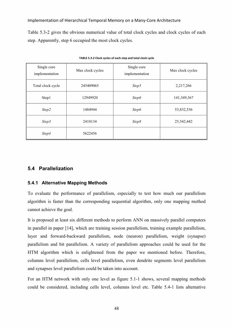
Implementation of Hierarchical Temporal Memory on a Many-Core Architecture
48
Table 5.3-2 gives the obvious numerical value of total clock cycles and clock cycles of each
step. Apparently, step 6 occupied the most clock cycles.
TABLE 5.3-2 Clock cycles of each step and total clock cycle
Single core
implementation Max clock cycles
Single core
implementation Max clock cycles
Total clock cycle 245409065 Step5 2,217,266
Step1 12949920 Step6 141,349,367
Step2 1484944 Step6 53,832,536
Step3 2410134 Step8 25,542,442
Step4 5622456
5.4 Parallelization
5.4.1 Alternative Mapping Methods
To evaluate the performance of parallelism, especially to test how much our parallelism
algorithm is faster than the corresponding sequential algorithm, only one mapping method
cannot achieve the goal.
It is proposed at least six different methods to perform ANN on massively parallel computers
in parallel in paper [14], which are training session parallelism, training example parallelism,
layer and forward-backward parallelism, node (neuron) parallelism, weight (synapse)
parallelism and bit parallelism. A variety of parallelism approaches could be used for the
HTM algorithm which is enlightened from the paper we mentioned before. Therefore,
columns level parallelism, cells level parallelism, even dendrite segments level parallelism
and synapses level parallelism could be taken into account.
For an HTM network with only one level as figure 5.1-1 shows, several mapping methods
could be considered, including cells level, columns level etc. Table 5.4-1 lists alternative

Implementation
49
mapping methods. For columns level parallelism, we propose four mapping methods, single
column mapping, block-based mapping, column-based mapping and row-based mapping.
TABLE 5.4-1 Alternative mapping methods
Column
Level
Single Column Distributed each column to a sequential processor core.
Block-Based Separate an HTM region into several blocks with an equal number of columns,
each or equal number of which are distributed to one processor core.
Column-Based Distribute every column of HTM columns to one processor core, or distribute
an equal number of columns of HTM columns to one processor core.
Row-Based Distribute every row of HTM columns to one processor core, or distribute an
equal number of rows of HTM columns to one processor core.
Cell Level Distribute each cell to one core of a many-core architecture
Dendrite Segment Level Distribute every dendrite segment to one core of a many-core architecture
Synapse Level Distribute a certain number of synapses to one core of a many-core architecture
Partially Parallelism Only parallel dominant part
5.4.2 Selected Columns Level Mapping Methods
The HTM algorithm has computing in columns and cells level which results in a large number
of ‘for’ loops operation in C programming. Therefore, HTM is well suited for parallel
implementing in many-core architecture. The HTM network established in this project is a
two dimensional network with a region of 16 by 16 columns, each of which includes 4 cells,
however the given many-core hardware platform has only 16 processor cores, in spite of the
fact that it could be scalable up to 4096 cores. If there are more cores used to implement HTM
algorithm, for instance 1024 cores, then an HTM network with 16*16*4 cells (1024 cells)
could be implemented in a parallel version in the cells level. For this thesis project, the
columns level parallelization is chosen to be implemented in the hardware with 16-cores,
which means each core will simulate 64 cells. The selected three mapping methods based on
columns level will be represented as follows.

Implementation of Hierarchical Temporal Memory on a Many-Core Architecture
50
Block-Based Mapping Method
The first mapping method is block-based, each block including 4 * 4 columns distributed to
an Epiphany core to process, in total including 16 blocks, which is illustrated in figure 5.4-1.
Each core implements one block of columns marked in dark blue, while 16 cores execute
simultaneously.
FIGURE 5.4-1 Block-Based Mapping Method
Column-Based Mapping Method
The second mapping method is column-based, each row of HTM columns distributed into one
core to implement, which is shown in figure 5.4-2. Each core implements one row of columns
marked in dark blue, while 16 cores executed simultaneously.
FIGURE 5.4-2 Column-Based Mapping Method
Row-Based Mapping Method
The third mapping method is row-based, each row of HTM columns distributed into one core
to implement, which is shown in figure 5.4-3. Each row of columns is executed by one
Epiphany core marked in dark blue.

Implementation
51
FIGURE 5.4-3 Row-Based Mapping Method
5.4.3 Communication and Synchronization
When implement an application on many-core architecture in a parallel version,
communication regardless of from host-PC to the many-core architecture or inter-cores
communication and synchronization, are always needed. In our task, the host-PC write 16 by
16 pixels image to shared memory, then it set all cores to run. In the running process, each
core does its own job, then waiting. The host-PC collects all the data in order when all cores
end of run, then it sets all cores continue to run. In the entire process, cores can read the data
simultaneously from the shared memory, but only one core can write the data to the shared
memory at any time.
In our task, data has dependencies, for example when the HTM network perform the training
image ‘A’, each core after running should waiting for other cores with which have the
dependencies, showing in figure 5.4-4. In our task, the inhibition radius equals to 1 and the
learning radius equals to 7. When we use the block-based mapping method to implement the
HTM on Epiphany, the HTM columns are separated into 16 blocks distributed to each core
and every core has different number of active columns and cells. If the image ‘A’ is trained by
HTM depending on this mapping method, the pixels are also separated to corresponding cores.
Blocks with no active input data will not activate corresponding HTM columns and cells,
consequently, the cores will have no work to do. Blocks with lots of active input data will
activate corresponding HTM columns and cells, these cores then will have much job to deal
with. Each core does its own job, waiting for other cores finished, after that goes to next step.
Because each column has an inhibition radius, and each cell has a learning radius, the
dependencies should be taken into account.

Implementation of Hierarchical Temporal Memory on a Many-Core Architecture
52
FIGURE 5.4-4 Dependencies of training data
5.5 Simulation in OpenMP
Open Multiprocessing[16], usually called OpenMP, is a multi-threading API that supports
multi-platform shared memory parallel programming in C, C++. Using OpenMP to implement
parallel application gives programmers a simple and flexible interface, because OpenMP
provides a portable, scalable platform. The parallelized section of shared-memory programs is
executed by multiple independent threads on one or more processors and some or all of the
available memory are shared. OpenMP provides a way for starting up threads, dividing work
to each thread to execute and coordinating synchronization.
The main aim of our thesis project is to implement the HTM algorithm on a many-core
architecture. Therefore, the extra experiment of simulating the HTM by OpenMP just want to
see how much the speedup is by simulating in OpenMP and compares the speedup and
efficiency with our implementation result on the proposed many-core architecture.
The HTM algorithm is simulated in a computer with 2 cores, each of which contains 2 threads,
4 threads in total and the computer is Intel® Core™ i5 CPU M 430 @ 2.27GHz × 4. Using
OpenMP can make the implementation automatic parallelization. Table 5.5-1 shows the
concrete data of OpenMP implementation. Figure 5.5-1 and figure 5.5-2 illustrates the
simulation result of parallel implementing HTM algorithm using OpenMP to process two
training sets respectively. The speedup is very low when simulates the HTM by OpenMP. If
using a computer with more threads to simulate by OpenMP, we inferred that the performance
probably reduced with the threads increased.

Implementation
53
TABLE 5.5-1 Result of OpenMP implementation of HTM algorithm
The number of threads Executiong time (ms) Speedup
1 thread 63647 1.0000
2 threads 42066 1.5137
3 threads 32606 1.9528
4 threads 31026 2.0523
FIGURE 5.5-1 Simulation in OpenMP of small training set FIGURE 5.5-2 Simulation in OpenMP of 20800 trains
Phase1 is the dominant part of implementing the small training example) (Phase2 is the dominant part of implementing the full training example)

Implementation of Hierarchical Temporal Memory on a Many-Core Architecture
54

Result Analysis
55
6 Results Analysis
Chapter 5 depicts different mapping methods and two experiments with different sizes of
problems have been done. This chapter then will give an analysis of the project results. The
result and analysis of the first experiment with small training examples will be described in
section 6.1, and following that section, the result and analysis of the second experiment with
full training examples will be described. Then follows a section will detail the execution time
of every training example with the full training set. In section 6.4, we will give a short
analysis of the communication between host-PC and hardware. The usefulness of the
hardware will be analyzed in section 6.5.
6.1 Result and Analysis of the Experiment with the Small Training Set
This project has done a parallel implementation of the HTM algorithm on the Adapteva
Epiphany many-core architecture with up to 16 cores using three different mapping methods
and the best mapping method has been determined. Moreover, in order to evaluate the
scalability of this parallel system, a trial of parallel implementation of the HTM algorithm on
different number of Epiphany cores has been performed by using the best mapping method.
6.1.1 Parallel Implementation on 16 Cores
Since three mapping methods have been implemented when using 16 cores to implement the
HTM algorithm, each parallel method leads to different execution result.
Result of Block-Based Mapping Methods
Figure 6.1-1 illustrates eight steps of HTM implementation on Adapteva Epiphany using 16
cores simultaneously for each step. The max clock cycle of this mapping method is 19319505.
Speedup of each step is illustrated in figure 6.1-1. From figure 6.1-1 we can see that in the
first five steps all cores are utilized almost evenly, however some of the 16 cores is only used
to implement less clock cycle from step6 to step7. Step6, which occupies most of the
execution time, thus, is the dominant part of the HTM algorithm. Of the total execution time
step6 takes 62.9%, but the utilization percentage of the cores is not that high. As step6 is so

Implementation of Hierarchical Temporal Memory on a Many-Core Architecture
56
dominant, the overall speedup of the block-based mapping is equal to the speedup of step6,
7.3146, thus the efficiency is then 0.4573.
FIGURE 6.1-1 Execution time of the block-based mapping method of the first experiment
FIGURE 6.1-2 Speedup of the block-based mapping method of the first experiment

Result Analysis
57
Result of Column-Based Mapping Method
Figure 6.1-3 illustrates the execution progress by distributing each column of HTM columns
to one Epiphany core to implement. Speedup of each step is illustrated in figure 6.1-4.
FIGURE 6.1-3 Execution time of the column-based mapping method of the first experiment
It is very obviously that from step1 to step5, the execution time of each core is approximately
the same. Step6 still accounted for the majority of execution time, but we see high utilization
of cores to be concentrated on the middle four processors. Table 6.1-1 gives the clock cycle
and calculated speedup of this mapping method, which is 25949537 and 5.4471 respectively.
The speedup is lower than the first mapping method. The efficiency of it is only 0.3404,
which means the cores are not utilized well.
Result of Row-Based Mapping Methods
Figure 6.1-5 and Figure 6.1-6 gives the illustration of the third parallel method, row-based
mapping, which distributes each row of HTM columns to one core. It can be seen from
figure6.1-5, 16 cores are utilized evenly in each step. The clock cycles is only 10175309, and
the speedup showed in figure 6.1-6 is up to 13.8914, which is close to 16, the ideal speedup,
more than the results of those two mappings. Its efficiency 0.8682 is highest among these
three parallel methods. Thus it can be seen that the 16 cores are well-utilized.

Implementation of Hierarchical Temporal Memory on a Many-Core Architecture
58
FIGURE 6.1-4 Execution time of the row-based mapping method of the first experiment
TABLE 6.1-1 Evaluation of three mapping methods implemented on 16 cores using the small training set
Table 6.1-1 summarizes the data that was collected and calculated from implementation on 16
cores of three mapping methods. It can be seen from above results that to make a parallel
implementation of the HTM algorithm by using the row-based mapping method can take
advantage of all cores with a high utilization in this experiment and gained a preferable
speedup.
For this small training set, the big difference between these three mapping methods is a result
of training example variability. The input pattern activity will lead to different columns and
cells active in the HTM network. Processors with less work will perform faster and have to
Mapping Method Max clock cycles Speedup Efficiency
Sequential
implementation 141,349,367 1.0000 1.0000
Block-Based 19,319,505 7.3164 0.4573
Column-Based 25,949,537 5.4471 0.3404
Row-Based 10,175,309 13.8914 0.8682

Result Analysis
59
wait for the slower ones to finish. When using idle processors to do other jobs, the whole
execution time would be reduced. This is because in this experiment, there exists uneven
distribution that the number of active columns assigned in each core is different. To be more
specific, processors may be assigned active columns need more time to execute because they
have active cells with a large number of active dendrite segments, while processors may be
assigned inactivated columns only need a little time to implement because they have no active
cells with nothing dendrite segments active.
The number of active columns distributed to each cores is almost equal in the row-based
mapping method. Therefore, it has the highest efficiency among these three parallel methods.
If the number of active columns varies a lot when distributed to each core, the execution time
of each core becomes uneven, consequently leading to low efficiency.
Because the row-based mapping method of the experiment gives the best performance, we
tried to implement the algorithm on 2 cores, 4 cores and 8 cores using this mapping method
respectively to evaluate the scalability, the results of which will represented in section 6.1.2.
6.1.2 Evaluation of Row-Based Mapping Method in the Experiment
This section gives the results of implementing the HTM algorithm by using the row-based
mapping method to two cores, four cores and eight cores respectively in order to see the
scalability of this parallel system. If 8 cores are used to parallel, every 2 rows of HTM
columns are distributed to each Epiphany core. The rest can be done in the same manner.
Table 6.1-2 gives the data of maximum clock cycles, speedup and efficiency.
TABLE 6.1-2 Evaluation of implementation the small training set
on different number of cores using row-based mapping
The number of cores Max clock cycles Speedup Efficiency
1 core 141,349,376 1.0000 1.0000
2 cores 74,022,835 1.9095 0.9548
4 cores 38,156,642 3.7044 0.9261
8 cores 20,118,246 7.0259 0.8782
16 cores 10,175,309 13.8914 0.8682

Implementation of Hierarchical Temporal Memory on a Many-Core Architecture
60
Apparently, the efficiency of the HTM implementation on different numbers of Epiphany
cores is different. To implement the HTM in 2 Epiphany cores through processing the pattern
recognition task resulted in the highest efficiency 0.9548, because every 8 rows of columns
including the similar number of active HTM columns are distributed into one core.
FIGURE 6.1-5 Speedup of implementation the small training set
on different number of cores using row-based mapping method
FIGURE 6.1-6 Efficiency of implementation the small training set
on different number of cores using row-based mapping methods
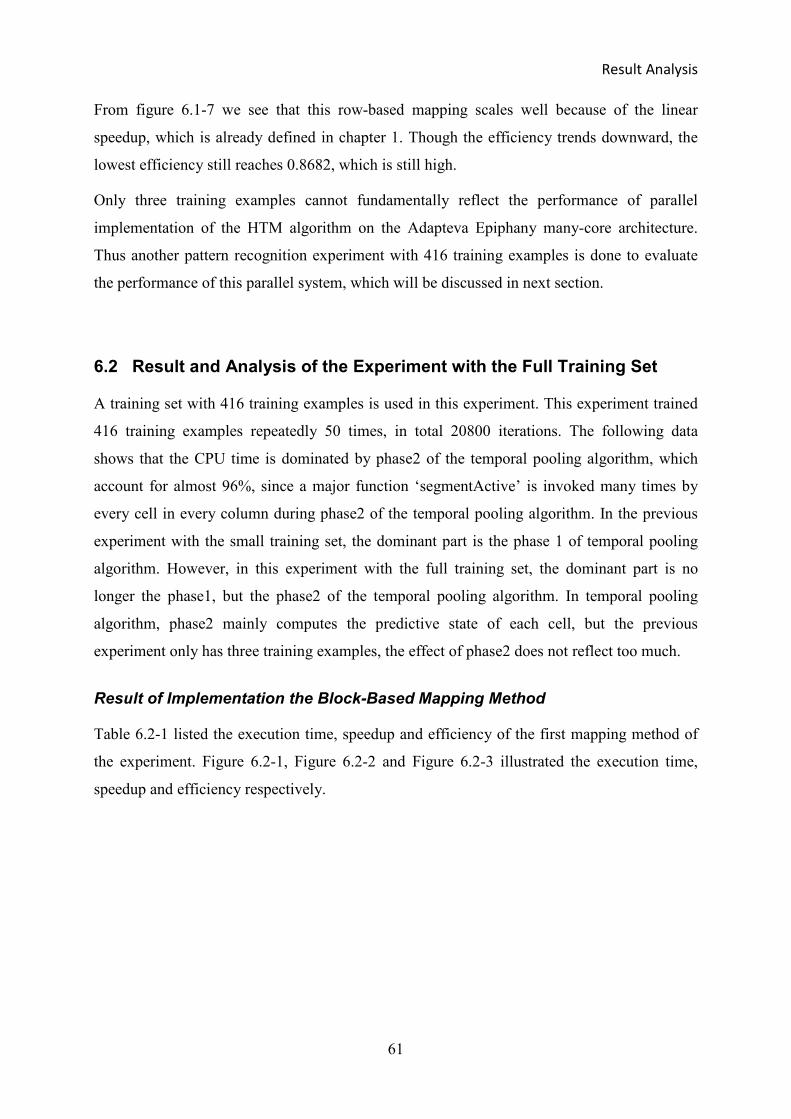
Result Analysis
61
From figure 6.1-7 we see that this row-based mapping scales well because of the linear
speedup, which is already defined in chapter 1. Though the efficiency trends downward, the
lowest efficiency still reaches 0.8682, which is still high.
Only three training examples cannot fundamentally reflect the performance of parallel
implementation of the HTM algorithm on the Adapteva Epiphany many-core architecture.
Thus another pattern recognition experiment with 416 training examples is done to evaluate
the performance of this parallel system, which will be discussed in next section.
6.2 Result and Analysis of the Experiment with the Full Training Set
A training set with 416 training examples is used in this experiment. This experiment trained
416 training examples repeatedly 50 times, in total 20800 iterations. The following data
shows that the CPU time is dominated by phase2 of the temporal pooling algorithm, which
account for almost 96%, since a major function ‘segmentActive’ is invoked many times by
every cell in every column during phase2 of the temporal pooling algorithm. In the previous
experiment with the small training set, the dominant part is the phase 1 of temporal pooling
algorithm. However, in this experiment with the full training set, the dominant part is no
longer the phase1, but the phase2 of the temporal pooling algorithm. In temporal pooling
algorithm, phase2 mainly computes the predictive state of each cell, but the previous
experiment only has three training examples, the effect of phase2 does not reflect too much.
Result of Implementation the Block-Based Mapping Method
Table 6.2-1 listed the execution time, speedup and efficiency of the first mapping method of
the experiment. Figure 6.2-1, Figure 6.2-2 and Figure 6.2-3 illustrated the execution time,
speedup and efficiency respectively.

Implementation of Hierarchical Temporal Memory on a Many-Core Architecture
62
TABLE 6.2-1 Efficiency evaluation of The Block-Based Mapping method with the full training set
FIGURE 6.2-1 Execution time of the block-based mapping method with the full training set
The number
of cores
Total
Execution time
(Minutes)
Phase 2
Execution time
(Minutes)
Total
Speedup
Phase 2
Speedup
Total
Efficiency
Phase 2
Efficiency
1 core 448.0667 437.1750 1.0000 1.0000 1.0000 1.0000
2 cores 228.6833 223.0167 1.9593 1.9603 0.9797 0.9801
4 cores 118.3667 115.2667 3.7854 3.7927 0.9464 0.9482
8 cores 62.9583 61.0250 7.1169 7.1639 0.8896 0.8955
16 cores 32.7583 31.5750 13.6779 13.8456 0.8549 0.8654

Result Analysis
63
FIGURE 6.2-2 Speedup of the block-based mapping method with the full training set
FIGURE 6.2-3 Phase 2 efficiency of the block-based mapping method with the full training set

Implementation of Hierarchical Temporal Memory on a Many-Core Architecture
64
Figure 6.2-1 shows the execution time of the block-based mapping method. The total
execution time is represented in green, while the execution time of phase2 is represented in
blue. It is easy to see that the execution time of phase2 almost occupies the total execution
time, which signifies that phase2 of the temporal pooling algorithm plays an essential role in
this experiment.
From figure 6.2-2 we can see that the speedup increases almost linearly with increasing the
number of cores when training 416 examples 50 times and nearly close to the ideal linearly
scalable line which is represented by the red dashed line, which reflects that the system is
scalable.
Figure 6.2-3 gives an obvious description of efficiency. The efficiency of parallel
implementation on different numbers of cores using the block-based mapping method is not
constant. It declines quickly from implementing on 1 core to 8 cores, but decreases more
slowly from 8 cores to 16 cores, however, the efficiency is still high, higher than 0.86 when
parallel implementation on 16 cores. From this result, we suspect that the following trend of
efficiency will be stable in a certain range with the increasing number of cores.
The data of the column-based mapping method and row-based mapping method is listed in
Table 6.2-2 and Table 6.2-3, which have only a little difference with the block-mapping
method, thus the similar figure of execution time, speedup, as well as efficiency will not be
shown below.
Result of Implementation the Column-based Mapping Method
TABLE 6.2-2 Efficiency evaluation of the column-based method
The number
of cores
Total
Execution time
(Minutes)
Phase 2
Execution time
(Minutes)
Total
Speedup
Phase 2
Speedup
Total
Efficiency
Phase 2
Efficiency
1 core 448.0667 437.1750 1.0000 1.0000 1.0000 1.0000
2 cores 228.6833 223.0167 1.9593 1.9603 0.9797 0.9801
4 cores 117.3583 114.2583 3.8179 3.8262 0.9545 0.9565
8 cores 62.3083 60.4250 7.1911 7.2350 0.8989 0.9044
16 cores 31.9833 30.8563 14.0094 14.1672 0.8756 0.8854

Result Analysis
65
Result of Implementation the Row-Based Mapping Method
TABLE 6.2-3 Efficiency evaluation of the row-based method
The number
of cores
Total
Execution time
(Minutes)
Phase 2
Execution time
(Minutes)
Total
Speedup
Phase 2
Speedup
Total
Efficiency
Phase 2
Efficiency
1 core 448.0667 437.1750 1.0000 1.0000 1.0000 1.0000
2 cores 228.0917 222.4250 1.9644 1.9655 0.9822 0.9877
4 cores 116.8167 113.7167 3.8356 3.8444 0.9589 0.9611
8 cores 62.0167 60.3083 7.2249 7.2490 0.9031 0.9061
16 cores 31.8083 30.7417 14.0791 14.2209 0.8799 0.8888
From the execution time tables above we see very little distinction between the different
mapping methods, when the large training set is used. When the HTM network processes a
pattern recognition task with a large amount of image sequences continuously using different
mapping methods, the impact of training set variability becomes not very evident, because the
number of active columns distributed in each cores are almost identical in any period of time.
However, the best speedup is still generated by the row-based mapping method.
For processing a large number of data, it can acquire a preferable performance through
making parallel implementation of HTM according to the row-based mapping method which
allocates each row of HTM columns into one processor core. This parallel system is scalable,
because the increase of speedup is linear of these three mappings, but row-based mapping is a
little better than the others.
6.3 Execution Time of Every Training Example with the Full Training Set
The last experiment calculates the execution time of training every pattern every time in order
to compare the differences between each mapping to see which one is the most sufficiently
stable mapping method. The following figures only show the results of the block-based
mapping method, because the results of three mappings are similar, but the detailed data will
be listed in a table below.
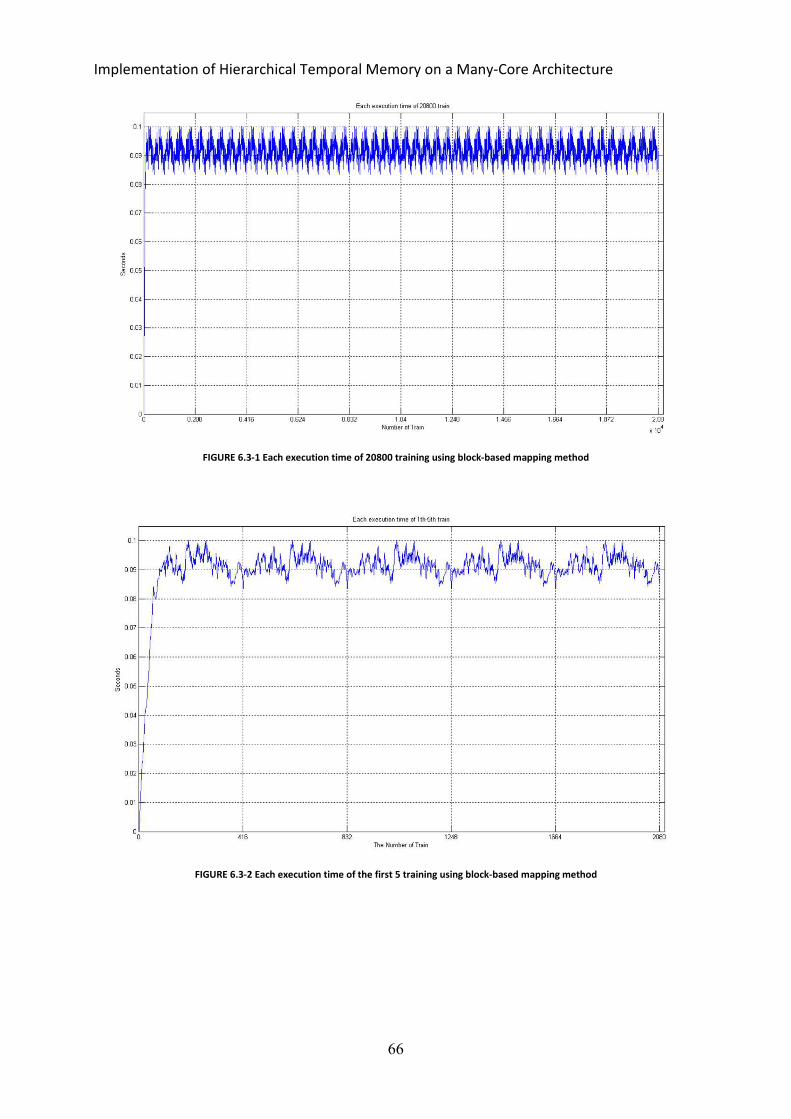
Implementation of Hierarchical Temporal Memory on a Many-Core Architecture
66
FIGURE 6.3-1 Each execution time of 20800 training using block-based mapping method
FIGURE 6.3-2 Each execution time of the first 5 training using block-based mapping method

Result Analysis
67
FIGURE 6.3-3 Execution time of 5th
and 45th
training using block-based mapping method
Figure 6.3-1 clearly shows the execution time of every training example in the full training set
by making parallel implementation of HTM on 16 cores. The full training set is trained 50
times and we will use “round” instead “time” in the following in order to avoid ambiguity. It
is obvious that the execution time of the first round of training increases continuously which
is illustrated in figure6.3-2, because of the number of segments increases as incrementing the
number of training examples. However, the execution time stops increasing after training the
416 examples once, but fluctuates within a certain range throughout the last 49 rounds of
training, due to the fact that the number of segments has already increased to the most, during
the first round of training. Since training examples contain different patterns with different
amount of information that need different times to process, a fluctuation within a specific
range has existed during every round of training. It is a periodic cycle from the 3rd
training to
the 50th
training according to a period with 416, which can be seen as steady state. Because
the 2nd
training might be influenced more or less by the startup phase (the first round of
training), it is not included in the steady state. During the last 48 rounds of repeated training,
the total execution time of every training period is similar, hence the waveforms repeat
periodically according to a period of 416.
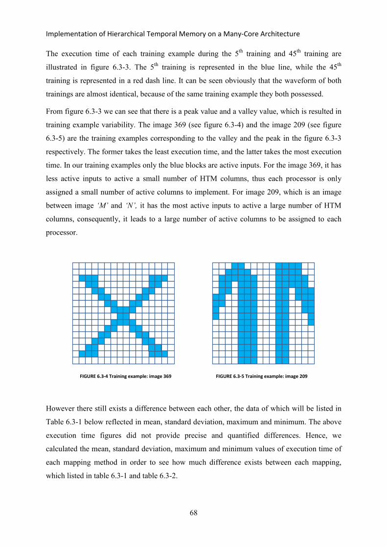
Implementation of Hierarchical Temporal Memory on a Many-Core Architecture
68
The execution time of each training example during the 5th
training and 45th
training are
illustrated in figure 6.3-3. The 5th
training is represented in the blue line, while the 45th
training is represented in a red dash line. It can be seen obviously that the waveform of both
trainings are almost identical, because of the same training example they both possessed.
From figure 6.3-3 we can see that there is a peak value and a valley value, which is resulted in
training example variability. The image 369 (see figure 6.3-4) and the image 209 (see figure
6.3-5) are the training examples corresponding to the valley and the peak in the figure 6.3-3
respectively. The former takes the least execution time, and the latter takes the most execution
time. In our training examples only the blue blocks are active inputs. For the image 369, it has
less active inputs to active a small number of HTM columns, thus each processor is only
assigned a small number of active columns to implement. For image 209, which is an image
between image ‘M’ and ‘N’, it has the most active inputs to active a large number of HTM
columns, consequently, it leads to a large number of active columns to be assigned to each
processor.
FIGURE 6.3-4 Training example: image 369 FIGURE 6.3-5 Training example: image 209
However there still exists a difference between each other, the data of which will be listed in
Table 6.3-1 below reflected in mean, standard deviation, maximum and minimum. The above
execution time figures did not provide precise and quantified differences. Hence, we
calculated the mean, standard deviation, maximum and minimum values of execution time of
each mapping method in order to see how much difference exists between each mapping,
which listed in table 6.3-1 and table 6.3-2.
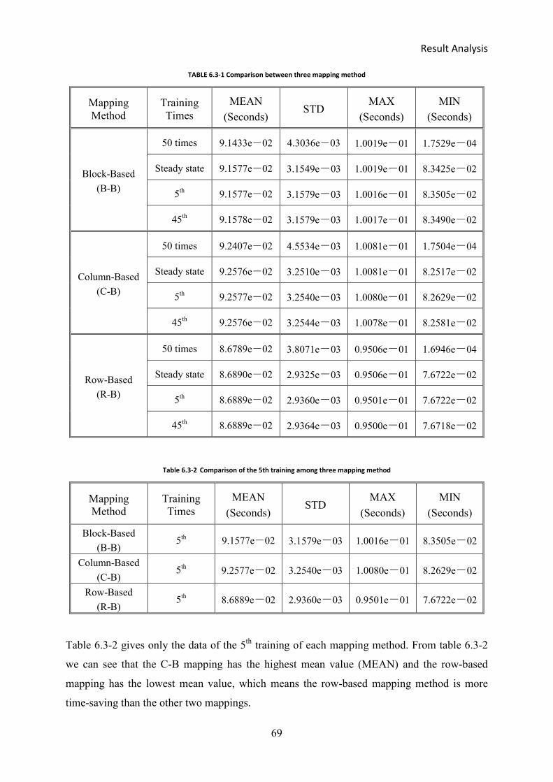
Result Analysis
69
TABLE 6.3-1 Comparison between three mapping method
Mapping
Method
Training
Times
MEAN
(Seconds) STD
MAX
(Seconds)
MIN
(Seconds)
Block-Based
(B-B)
50 times 9.1433e-02 4.3036e-03 1.0019e-01 1.7529e-04
Steady state 9.1577e-02 3.1549e-03 1.0019e-01 8.3425e-02
5th 9.1577e-02 3.1579e-03 1.0016e-01 8.3505e-02
45th 9.1578e-02 3.1579e-03 1.0017e-01 8.3490e-02
Column-Based
(C-B)
50 times 9.2407e-02 4.5534e-03 1.0081e-01 1.7504e-04
Steady state 9.2576e-02 3.2510e-03 1.0081e-01 8.2517e-02
5th 9.2577e-02 3.2540e-03 1.0080e-01 8.2629e-02
45th 9.2576e-02 3.2544e-03 1.0078e-01 8.2581e-02
Row-Based
(R-B)
50 times 8.6789e-02 3.8071e-03 0.9506e-01 1.6946e-04
Steady state 8.6890e-02 2.9325e-03 0.9506e-01 7.6722e-02
5th 8.6889e-02 2.9360e-03 0.9501e-01 7.6722e-02
45th 8.6889e-02 2.9364e-03 0.9500e-01 7.6718e-02
Table 6.3-2 Comparison of the 5th training among three mapping method
Mapping
Method
Training
Times
MEAN
(Seconds) STD
MAX
(Seconds)
MIN
(Seconds)
Block-Based
(B-B) 5
th 9.1577e-02 3.1579e-03 1.0016e-01 8.3505e-02
Column-Based
(C-B) 5
th 9.2577e-02 3.2540e-03 1.0080e-01 8.2629e-02
Row-Based
(R-B) 5
th 8.6889e-02 2.9360e-03 0.9501e-01 7.6722e-02
Table 6.3-2 gives only the data of the 5th
training of each mapping method. From table 6.3-2
we can see that the C-B mapping has the highest mean value (MEAN) and the row-based
mapping has the lowest mean value, which means the row-based mapping method is more
time-saving than the other two mappings.

Implementation of Hierarchical Temporal Memory on a Many-Core Architecture
70
The standard deviation (STD) shows how much variation or "dispersion" exists from the mean.
A low standard deviation indicates that the data points tend to be very close to the mean,
whereas high standard deviation indicates that the data points are spread out over a large
range of values. C-B mapping has the highest standard deviation among these three mapping
methods, which indicates that it has high volatility.
The R-B mapping has the minimum average among three mappings, and it has the lowest
standard deviation. For the R-B mapping, the standard deviation of the steady state or the 5th
training or the 45th
training, there only exists a little variance among them, even the variance
can be ignored, which means the R-B mapping is the most sufficiently stable mapping method
among three mapping methods.
From the macro view, the existing tiny difference between each mapping method can be
ignored. Therefore, for the three mapping methods, we can say that they have the similar
performance with well scalability and high efficiency.
6.4 Analysis of Communication between Host-PC and Hardware
The proposed many-core architecture, Epiphany, is a shared memory system. There are three
main programming notions, task creation, communication, and synchronization in a
programming model in shared memory systems [16]. In a shared memory many-core platform,
communication among parallel processes is executed through writing to and reading from the
shared variables in the shared data segments.
When we implement the HTM algorithm on the Epiphany hardware, the communication
between host-PC and Epiphany is essential. In the first experiment with a small training set,
three image sequences are performed by the HTM network, and the algorithm is separated to
several steps. When each step finished, the host-PC needs to communicate with the hardware
once, in total seven communications were made while training one image sequence. When the
HTM is implemented on 16 cores, the host-PC reads data from hardware from the first core to
the last core in order rather than collecting data from cores which finish earlier to others
which performed more slowly. Consequently, it spends a lot of time. The total execution time
of the experiment with a small training set is only approximately two seconds, but the time we
spent on implementing is about 10 minutes which is 300 times of the execution time. If we
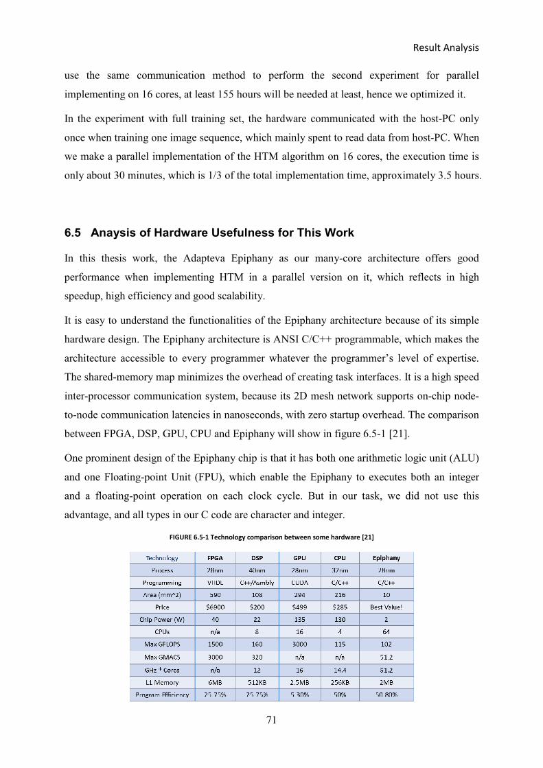
Result Analysis
71
use the same communication method to perform the second experiment for parallel
implementing on 16 cores, at least 155 hours will be needed at least, hence we optimized it.
In the experiment with full training set, the hardware communicated with the host-PC only
once when training one image sequence, which mainly spent to read data from host-PC. When
we make a parallel implementation of the HTM algorithm on 16 cores, the execution time is
only about 30 minutes, which is 1/3 of the total implementation time, approximately 3.5 hours.
6.5 Anaysis of Hardware Usefulness for This Work
In this thesis work, the Adapteva Epiphany as our many-core architecture offers good
performance when implementing HTM in a parallel version on it, which reflects in high
speedup, high efficiency and good scalability.
It is easy to understand the functionalities of the Epiphany architecture because of its simple
hardware design. The Epiphany architecture is ANSI C/C++ programmable, which makes the
architecture accessible to every programmer whatever the programmer’s level of expertise.
The shared-memory map minimizes the overhead of creating task interfaces. It is a high speed
inter-processor communication system, because its 2D mesh network supports on-chip node-
to-node communication latencies in nanoseconds, with zero startup overhead. The comparison
between FPGA, DSP, GPU, CPU and Epiphany will show in figure 6.5-1 [21].
One prominent design of the Epiphany chip is that it has both one arithmetic logic unit (ALU)
and one Floating-point Unit (FPU), which enable the Epiphany to executes both an integer
and a floating-point operation on each clock cycle. But in our task, we did not use this
advantage, and all types in our C code are character and integer.
FIGURE 6.5-1 Technology comparison between some hardware [21]

Implementation of Hierarchical Temporal Memory on a Many-Core Architecture
72

Conclusion and Suggestion to The Future Work
73
7 Conclusion and Suggestion to the Future Work
7.1 Conclusion
HTM is a complex algorithm which models the function of human brain. In this thesis, we
programmed an HTM network in C and mapped onto the Adapteva Epiphany many-core
hardware. This parallel implementation of HTM running on the selected many-core hardware
significantly reduced the computing time compared to an implementation on a singe-core
computer.
In this thesis, three column level mapping methods which are block-based, column-based, and
row-based parallelization is selected from five parallel methods to perform HTM, because the
provided Epiphany many-core hardware has only 16 cores, which is not enough to parallel in
cells level, let alone parallel in dendrites level and synapses level. the HTM algorithm on the
Adapteva Epiphany.
In our thesis, the performance of HTM’s parallel implementation is evaluated through
comparing speedup, efficiency and scalability. In the experiment with the small training set,
there exists big difference between the results of the three mapping methods because of the
training example variability and the row-based mapping method gives the best performance.
For the experiment with the full training set we did not see this effect, instead all three
mappings have almost identical results. The impact of training examples variability becomes
not very apparent in this experiment, because the number of active columns distributed in
each core is almost identical in any period of time.
To compare the corresponding results from Adapteva Epiphany implementation and OpenMP
(2 cores with 2 threads, 4 cores with 4 threads), the performance of Epiphany implementation
far outweighs the one coming from OpenMP. The good performance we gained from HTM’s
Adapateva Epiphany implementation because of its advanced hardware and software design,
such as C programmable, 2D mesh network, 32 kilobytes of memory in each core, and some
others, which make contribute to the good performance of HTM’s parallel implementation.

Implementation of Hierarchical Temporal Memory on a Many-Core Architecture
74
7.2 Future Work
In this work we have only implemented an HTM algorithm without hierarchy using three
different mapping methods in a 16-core many-core architecture. There are still many aspects
of the HTM implementation that need to be optimized in the future, such as to construct a
multilayer HTM, to offer more optional mapping methods and several works about
implementation HTM on hardware can be done in the future.
In the future, one can try to implement a multilayer HTM and evaluate it through implement
high dimensional input data, such as RGB images. One can verify the correctness of inference
of the HTM network and to test its performance.
We have only done the HTM parallelization on columns level. In the future, one can also
evaluate other levels such as cells level or in dendrite segments level, and especially in
synapses level or find out more optional mapping methods. We selected three parallel models
to implement HTM on a 16-core many-core platform and discovered the dominant part.
Sometimes, the dominant part can be processed in a certain number of cores and other parts
could be executed using only a small number of cores to avoid the communication overhead.
We only have implemented HTM on 16 cores in a parallel version, and evaluated the
performance. In the future, it would be very worthwhile to try to implement HTM on a larger
Adapteva Epiphany with maybe hundreds or thousands of cores and use its functionality of
floating point, further more to evaluate the performance. It would be meaningful to know how
many cores at most are suitable for executing the HTM algorithm.
A preferable way to implement HTM is to discover hardware for HTM application in a
variety of domains with a high generalization. So one can try to implement HTM on other
many-core architectures, such as FPGA, or GPU and so on, in a parallel version and then
compare the performance with the parallel implementation of the HTM on Adapteva
Epiphany.

Reference
75
8 Reference
[1] J.Hawkins, S.Blakeslee, On Intelligence, New York: Times Books, 2004.
[2] Numenta, Hierarchical temporal memory including HTM cortical learning algorithms,
Technical report, Version 0.2.1, 2011.
[3] K.H.Seok, Y.S.Kim, “A new robot motion authoring method using HTM,”
International Conference on Control, Automation and Systems, pp. 2058-2061, 2008.
[4] W.Melis and M.Kameyama, “A study of the different uses of colour channels for traffic
sign recognition on hierarchical temporal memory,” Fourth International Conference
on Innovative Computing, Information and Control (ICICIC), pp. 111–114, 2009.
[5] W.J.C.Melis, S.Chizuwa and M.Kameyama, “Evaluation of the hierarchical temporal
memory as soft computing platform and its VLSI architecture”, 39th International
Symposium on Multiple-Valued Logic, pp. 233-238, 2009.
[6] J.Kwiatkowski, “Evaluation of parallel programs by measurement of its granularity,”
Proc. of the Conference on Parallel Processing and Applied Mathematics, Lecture
Notes in Computer Science, Vol. 2328, pp. 145-153, 2001.
[7] S.Akhter, J.Roberts, Multi-Core Programming, Intel Press, 2006.
[8] T.Hastie, R.Tibshirani and J.Friedman, The elements of statistical learning, data
mining, inference, and prediction, New York: Springer-Verlag, 2009.
[9] T.M.Mitchell, Machine learning, New York: McGraw-Hill, 1997.
[10] H.El-Rewini and M.Abd-El-Barr, Advanced Computer Architecture and Parallel
Processing (Wiley Series on Parallel and Distributed Computing) 1st ed., Wiley-
Interscience, 2005.
[11] Adapteva, Epiphany Architecture Reference, Adapteva Inc, 2008.
[12] S.Sriram, and S.S.Bhattacharyya, Embedded Multiprocessors Scheduling and
Synchronization, Embedded Multiprocessors: Scheduling and Synchronization, Marcel
Dekker, Inc., 2002.
[13] T. Nordström, B. Svensson, “Using and Designing Massively Parallel Computers for
Artificial Neural Networks”, Journal of parallel and distributed computing vol 14, 260-
285, 1992.
Implementation of Hierarchical Temporal Memory on a Many-Core Architecture
76
[14] L.Bengtsson, A.Linde, T.Nordstrom, B.Svensson, and M.Taveniku, “The REMAP
reconfigurable architecture: a retrospective, in FPGA implementations of neural
networks”, FPGA Implementations of Neural Networks, Springer Verlag, pp. 325-360,
2006.
[15] R.W.Price, “Hierarchical temporal memory cortical learning algorithm for pattern
recognition on multi-core architectures”, thesis of Portland State University, 2011.
[16] B. Chapman, G. Jost, and R. van der Pas, Using OpenMP: Portable Shared Memory
Parallel Programming. Cambridge, MA: MIT Press, 2008.
[17] D. Gove, Multicore Application Programming For Windows, Linux, and Oracle
Solaris, Addison-Wesley Educational Publishers Inc, 2011.
[18] Adapteva, Epiphany SDK Reference, Adapteva Inc, 2008.
[19] L, Gwennap, “Adapteva: More Flops, Less Watts, Epiphany Offers Floating-Point
Accelerators for Mobile Processors”, Mircoprocessor Report. June, 2011.
[20] D.O.Hebb, The organization of behavior. New York: John Wiley, 1949.
[21] Adapteva, Introduction, URL: http://www.adapteva.com/introduction/, available online.


