
Intelligent Vehicles Symposium (IV), 2014 IEEE
Improving GPS-Based Vehicle Positioning
for Intelligent Transportation Systems
Arghavan Amini1, Reza Monir Vaghefi2, Jesus M. de la Garza1, and R. Michael Buehrer2
Abstract— Intelligent Transportation Systems (ITS) haveemerged to utilize different technologies to enhance the perfor-mance and quality of transportation networks. Many applica-tions of ITS need to have a highly accurate location informationfrom the vehicles in a network. The Global Positioning System(GPS) is the most common and accessible technique for vehi-cle localization. However, conventional localization techniqueswhich mostly rely on GPS technology are not able to provide re-liable positioning accuracy in all situations. This paper presentsan integrated localization algorithm that exploits all possibledata from different resources including GPS, radio-frequencyidentification, vehicle-to-vehicle and vehicle-to-infrastructurecommunications, and dead reckoning. A localization algorithmis also introduced which only utilizes those resources that aremost useful when several resources are available. A close-to-real-world scenario has been developed to evaluate the perfor-mance of the proposed algorithms under different situations.Simulation results show that using the proposed algorithmsthe vehicles can improve localization accuracy significantly insituations when GPS is weak.
I. INTRODUCTION
The increasing need for mobility results in more traffic
and congestion in cities, suburban areas, and even interstate
highways. More vehicular traffic results in more accidents
and emergency situations. Many think building new roads
and repairing aging infrastructure are the best approaches for
addressing these problems [1]. However, a brighter future
for transportation can be obtained by using information
technology within the transportation system and making it
more intelligent. Intelligent Transportation Systems (ITS)
exploiting different synergistic technologies have emerged
to improve the safety and quality of transportation networks
[1]. ITS have many applications from collision warning
to law enforcement and environmental monitoring. Most
applications of the ITS rely on accurate location information
from the elements of the transportation network.
The most accessible vehicle navigation technique is the
Global Positioning System (GPS). However, it is well-known
that GPS cannot provide precise location information in
all situations [2]. In other words, GPS receivers are unre-
liable in dense environments (e.g., urban canyons), indoor
environments (e.g., parking garages, tunnels), or anywhere
else without a direct view to sufficient number of satellites.
However, several applications of ITS still require the location
1A. Amini and J. M. de la Garza are with the Department of Civiland Environmental Engineering, Virginia Tech, Blacksburg, VA 24061 [email protected], [email protected]
2R. M. Vaghefi and R. M. Buehrer are with the Department of Electricaland Computer Engineering, Virginia Tech, Blacksburg, VA 24061 [email protected], [email protected]
information of the elements in these places. Several tech-
niques have been proposed to enhance the performance of
GPS in such environments [3], [4].
Vehicular communications has been developed as a part
of ITS which enables vehicles to broadcast their vital in-
formation to the neighboring nodes including infrastruc-
ture (Vehicle-to-Infrastructure or V2I), vehicles (Vehicle-
to-Vehicle or V2V), and pedestrians (Vehicle-to-Pedestrian
or V2P). To facilitate less interference communication, the
United States Federal Communications Commission (FCC)
has allocated 75 MHz of spectrum in the 5.9GHz band to
vehicular communications which is referred to as Dedicated
Short-Range Communications (DSRC). Vehicular commu-
nications can be employed not only for data exchange but
also for positioning purposes. In particular, the infrastructure
can play the role of GPS satellites [5]. Note that V2I com-
munications refers to any form of communication between a
vehicle and a static device with an exact known location (the
so called anchor node). For instance, it can be done through
a DSRC between the On-Board Equipment (OBE) installed
in the vehicle and Roadside Equipment (RSE) installed at a
traffic light [6], through cellular communications between
the cellphone of the driver and the network base station
[7], [8], or through a wireless sensor network operating in
an unlicensed band [9], [10]. Similar to GPS, V2I commu-
nications can provide absolute vehicle locations. However,
building infrastructure for this purpose can be expensive.
Hence, V2V and V2P communications can be also used as
alternatives [4], [11], [12]. Incorporating V2V and V2P in
positioning is referred to as cooperative positioning where
a vehicle communicates to other nearby nodes and uses
their information to improve its location estimation [13]. It
has been shown that using V2V ranging along with GPS
can improve the positioning accuracy in comparison with
standalone GPS techniques [14] and [15]. However, V2V and
V2P communications can only provide relative positions of
the vehicles and not their absolute ones. Therefore, V2V and
V2P ranging would be beneficial only when vehicles have
their approximate locations from a GPS receiver or a static
device with an exact known location. In the case of a GPS
outage, vehicles do not have their approximate locations and
V2V and V2P communications cannot provide significant
improvement.
Another technique to enhance the accuracy of GPS lo-
calization is map matching [4], [16], [17], where several
databases including maps and information of the transporta-
tion network are incorporated in vehicle positioning. The
processing time of location estimation using this method is
typically high. Another disadvantage of these techniques is
that GPS reception is required to have a reasonable accuracy,
otherwise map matching would be useless.
Dead reckoning (DR) is another technique used to improve
the positioning accuracy. In DR, previous information (loca-
tion and velocity) is used to predict future information which
helps the vehicle find its location more precisely [18], [19].
However, similar to V2V communications, DR techniques
are useful only when GPS or a static device with exact known
location are used to provide the approximate locations of the
vehicle. The estimation error of DR techniques can be very
large when DR is being used for a long period of time in case
of GPS outage, as DR estimates the location of the vehicle
merely based on prediction and previous estimates.
Several studies suggest incorporating radio-frequency
identification (RFID) technology to improve the GPS accu-
racy [20], [21]. Although RFID results in more accurate lo-
calization, its performance relies heavily on GPS and would
not be reliable in cases where GPS outages can happen. This
technology can improve the positioning accuracy in places
where GPS access is limited. However, stand-alone RFID
cannot provide good accuracy indoors such as in parking
garages and tunnels where GPS receivers do not operate
at all.
In most of the studies mentioned above, an additional
resource (V2I, V2V,V2P, RFID, and DR) to the standalone
GPS is utilized to help the vehicle localize itself. Unlike
previous studies, this study is not restricted to only one of
the resources. An Integrated algorithm is proposed which
enables the vehicle to use all different positioning techniques
including GPS, RFID, V2I, and V2V. The proposed algo-
rithm does not merely rely on any individual signal, but
it can utilize them whenever any of them are available.
For instance, unlike most previous studies in which the
vehicle has to be connected to at least several GPS satellites,
the proposed algorithm uses GPS satellites only when they
are available and useful. A comprehensive evaluation and
comparison is conducted to demonstrate the effectiveness of
different positioning technologies for different environments.
We also studied the performance of the Integrated algo-
rithm in dense environments, such as Downtown Manhattan
in N.Y. In such environments, there are many vehicles present
in the areas and they need to be localized at sufficiently high
accuracy. Due to the large number of vehicles packed in a
small area, the vehicles may have many connections with
either infrastructure and/or other vehicles. The integrated
algorithm uses all connections to estimate the vehicle’s
location. However, sometimes the vehicle has many con-
nections and not all of them are necessarily useful. These
connections slow down the estimation process and do not
provide significant improvement. Therefore, an algorithm
(the so called Smart algorithm) is proposed which only
utilizes the most beneficial connections in estimating the
vehicles’ locations. The proposed Smart algorithm filters out
the redundant connections and keeps only those connections
that provide the desired accuracy. The proposed algorithms
are developed and simulated in MATLAB. A transportation
network scenario which includes several different situations
is created and the performance of the proposed algorithms
is evaluated through computer simulations.
II. METHODOLOGY
The main idea is to estimate the locations of the vehicles
from a series of range measurements obtained from GPS
satellites, V2I, V2V, and RFID connections. Moreover, the
algorithm is able to use DR to improve the localization
accuracy. Let xki = [xk
v,i, ykv,i, z
kv,i]
T be the location of the
ith vehicle at the kth time-step and ykj = [xk
u,j , yku,j, z
ku,j ] be
the location of jth unit at the kth time-step. Units refer to
GPS satellites, anchor nodes, or RFID readers. There are Nvehicles and M units in the network. Let Uk
i and Vki be sets
of indices of the units (except RFID readers) and vehicles
connected to the ith vehicle at kth time-step, respectively.
Let rkij be the range measurement between the ith vehicle
and the jth unit (except RFID readers) at the kth time-step.
Hence, it can be modeled as [2], [9]
rkij = dkij + nkij , j ∈ Uk
i
rkil = dkil + nkil, l ∈ Vk
i (1)
where dkij , dkil are the true distances, defined as:
dkij =√
(xkv,i − xk
u,j)2 + (ykv,i − yku,j)
2 + (zkv,i − zku,j)2
dkil =√
(xkv,i − xk
v,l)2 + (ykv,i − ykv,l)
2 + (zkv,i − zkv,l)2
and nkij , nk
il define the measurement noises which are
modeled as Gaussian random variables with variance σ2
ij
[22]. Typically, the lack of perfect synchronization between
the receiver and the GPS satellite [2] is considered by
adding an extra parameter (clock offset) to (1). For the
sake of simplicity, the effect of clock error is neglected
here. However, it does not change the relative performance
of the algorithms. The information obtained from an RFID
reader cannot be modeled as (1). RFID measurements can
be modeled as [23]:
dkij ≤ rkij , j ∈ Dki (2)
where Dki is the set of indices of the RFID readers connected
to the ith vehicle. rkij for RFID readers are defined by their
communication range. To consider DR, an underlying state
model for the movement of the vehicles should be defined.
Let vki = [vkx,i, v
ky,i, v
kz,i]
T be the velocity of the ith vehicle
at the kth time-step. The relationship between the previous
and current location of the vehicle can be modeled as [24],
[25]:
θki = Aθ
k−1
i +wki (3)
where θki = [xk
i ,vki ]
T, and
A =
[
I3 ∆I303 I3
]
.
wki defines the prediction error and is typically modeled as a
Gaussian random variable with variance Qkw,i. ∆ is the time-
step between two sets of measurements. 03 and I3 denote
the 3× 3 zero and identity matrices, respectively.
Now, the problem in hand is to estimate the location of
the vehicles from noisy range measurements in (1), data
from RFID readers in (2), and underlying state model in
(3). A maximum a posteriori estimation (MAP) algorithm is
used to estimate the locations of the vehicle from the range
measurements and underlying state model [26], while data
from RFID readers can act as a constraint on the estimation
problem [11], [27]. Therefore, the location of ith vehicle at
the kth time step is obtained from the following optimization
problem [11]:
minimizeθk
i
∑
j∈Uk
i
σ−2
ij
(
rkij − dkij)2
+∑
l∈Vk
i
σ−2
il
(
rkil − dkil)2
+(
θki − θ
k|k−1
i
)T (
Pk|k−1
i
)−1 (
θki − θ
k|k−1
i
)
subject to dkij ≤ rkij , j ∈ Dki
θk|k−1
i = Aθk−1|k−1
i ,
Pk|k−1
i = APk−1|k−1
i AT +Qkw,i (4)
where θk−1|k−1
i and Pk−1|k−1
i are the estimate and the
variance of the location and velocity of the vehicle at
the (k − 1)th time-step, respectively. The estimate of the
vehicle location and velocity at the current time-step is the
solution of (4). The details for determining the variance of
the estimate Pk|ki can be found in [11]. In the problem in
(4) the first, second, and third terms refer to vehicle-unit
measurements, vehicle-vehicle measurements, and internal
prediction, respectively. Moreover, the constraint in (4) refers
to vehicle-RFID connection. The optimization problem in (4)
does not have a closed-form solution. In the simulations, (4)
is solved with the MATLAB routine fmincon. The problem
in (4) can be solved in two ways: distributed and centralized
[28]. In the former, the location of all vehicles is estimated
simultaneously. In the latter, the location of each vehicle is
estimated individually. Therefore in this case, the location of
the desired vehicle is estimated by replacing the unknown
locations of other vehicles with their predicted ones in (4).
Although the centralized technique provides higher accuracy,
its complexity grows exponentially as the number of vehicles
increases. Hence, the distributed technique is employed here.
A. Smart Algorithm
Generally speaking, the more connections the vehicle has,
the higher the accuracy of the localization will be. On the
other hand, as the number of connections increases, the
complexity of the algorithm intensifies. In the problem in (4),
the vehicle is using all connections to estimate its location.
However, sometimes the vehicle has many connections and
not all of them are necessarily useful. These connections
slow down the estimation process and do not provide
significant improvement. This situation happens frequently
in dense environments where a large number of vehicles
are packed in a small area. In this case, a vehicle using
V2V communications would have many connections to the
other neighboring vehicles, most of them are not useful
though. The Smart algorithm described here filters out the
redundant connections and keeps only those connections that
provide the desired accuracy. The proposed Smart algorithm
processes the available connections and reports the useful
ones to the Integrated algorithm in (4).
To evaluate whether a set of connections provide the
desired accuracy or not the CramerRao lower bound (CRLB)
is used. The CRLB expresses a lower bound on the variance
of any unbiased estimator [26]. The CRLB is used as a
benchmark to evaluate the performance of unbiased estima-
tors. In other words, it tells us how accurate the estimator
is and how far its performance is from the lower bound.
The CRLB of the unknown variables to be estimated is
obtained from diagonal elements of the inverse of the Fisher
information matrix [26]:
CRLB([xki ]m) = [I(xk
i )−1]mm, m = 1, 2, 3. (5)
The detail for calculating the Fisher information matrix
(FIM) is provided in [11]. The CRLB of the location of
the desired vehicle depends on the locations of the satellites,
anchor nodes, and other vehicles connected to that vehicle
and the variance of the measurements. Since the locations of
other vehicles are unknown, the desired vehicle predicts their
locations based on the state model to calculate the CRLB.
The location of a vehicle consists of three variables (i.e., 3-D
coordinates, x, y, and z) and the overall accuracy is calcu-
lated as√
Trace{I(xki )
−1} [9]. Since RFID connections do
not provide range measurements, they cannot be included
in the CRLB. Therefore, in this case, we assume that the
vehicle only uses GPS, V2V, and V2I connections.
The proposed Smart algorithm is provided in Algorithm I.
Aki = Uk
i ∪ Vki is the set of all available connections at
the kth time-step and Cki be the set of connections selected
by the Smart algorithm (Cki ⊆ Ak
i ). Suppose at the kth time
step, Ck−1
i is available. In line 1, the algorithm calculates the
intersection of the set of connections obtained from the Smart
algorithm at the k − 1th time step and the set of available
connections at the kth time step. In line 2, the algorithm
calculates the Fisher information matrix using the set Cki . In
line 3, the difference between the desired accuracy, ǫ, and
the predicted accuracy√
Trace{I−1} is calculated. In line 4,
If the predicted accuracy is better than required accuracy,
δ < −0.15ǫ, the algorithm needs to remove a connection,
because the Smart algorithm anticipates that the selected
set Cki can provide better accuracy than the desired one.
However, the algorithm needs to determine which connection
should be removed from the set. Intuitively, it is better to
select the connection whose removal has the least impact on
the predicted accuracy. One way to calculate the effect of
removing or adding a connection on the predicted accuracy
is to calculate the CRLB for the new set of connections
from scratch. It typically takes a lot of processing time,
especially when the number of connections is high. However,
the Smart algorithm is only useful when the running time
of the connection selection process plus location estimation
based on those connections is less than that of the fully-
Integrated algorithm using all connections. Therefore, instead
Algorithm I. Smart Localization Algorithm
1. Cki← Ck−1
i∩ Ak
i
2. I← Fisher(Cki)
3. δ ←√I−1 − ǫ
4. if δ < −0.15ǫ then
5. remove the worst connection, j, from the set, Cki= Ck
i− j
6. elseif δ > 0.15ǫ then
7. add the best connection, j, to the set, Cki= Ck
i∪ j
8. else
9. do not change the set, Cki= Ck
i
10. end if
of calculating the CRLB of the new set, the following
approximation is used [29]:
(I+ ǫZ)−1 ≈ I−1 − ǫI−1ZI−1 (6)
where Z is the FIM of the connection to be removed. Since
matrix inversion is a complex process for large matrices,
the impact of a new connection can be simply calculated
by using above approximation (I−1ZI−1) which can be
determined significantly faster than calculating and inverting
a new FIM. Therefore, adding or removing the considered
connection changes the CRLB by I−1ZI−1. In this case, the
algorithm needs to remove a connection which has the least
effect on the accuracy. Therefore, a connection which has the
lowest value of Trace{I−1ZI−1} is removed from the set.
In line 6, if the predicted accuracy is worse than the
required accuracy, δ > 0.15ǫ, the algorithm needs to add
a connection to the set to compensate the lack of suffi-
cient accuracy. Similar to the previous case, selection of a
connection is performed based on the CRLB. However, in
this case, a connection which delivers the highest accuracy
improvement should be selected. Again, the algorithm starts
calculating I−1ZI−1 for all available connections and selects
the one that has the highest value of Trace{I−1ZI−1}. In
line 8, if the predicted accuracy falls between (0.85ǫ, 1.15ǫ),the algorithm proceeds without any changes. Note that a
15% tolerance is considered to prevent the algorithm from
unnecessary processing. The user can change the tolerance
depending on application requirements. Additional details
about the proposed Smart algorithm can be found in [11].
The practicality of the proposed positioning system is
dependent on two important components. First, a sufficient
number of sensors or other resources should be installed
along the roads to cover the areas that GPS fails. Although
such resources are not available immediately, new tech-
nologies and advancements make it possible in near future.
Second, since each positioning system works based on its
own requirements and specifications (e.g., ranging technique,
input and output information, and accuracy), a data fusion
center is also required to make data homogeneous and send
it to the algorithm.
III. SIMULATION RESULTS
In this section, the performance of the proposed algorithms
is evaluated through computer simulations. The proposed
transportation network and the traveling path of the desired
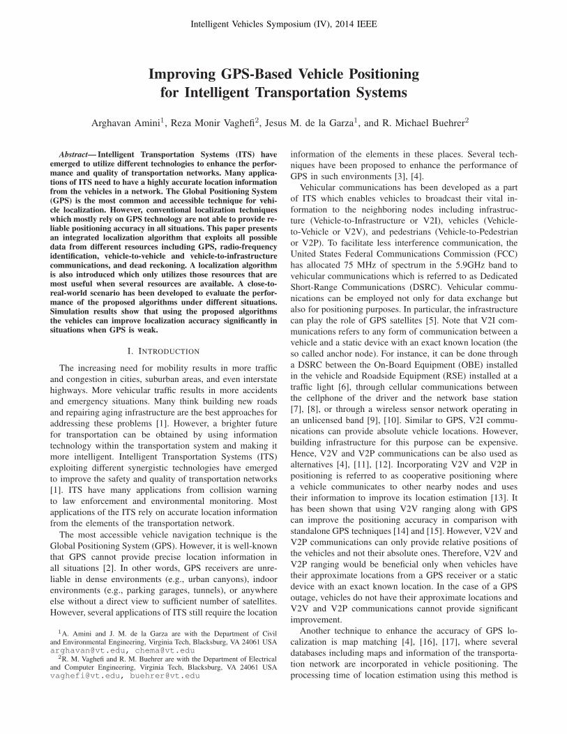
vehicle are depicted in Fig. 1a. Different conditions are
included in the simulated network. Several infrastructure and
RFID readers are considered around the road. There are
also 15 other vehicles in the network. The desired vehicle
experiences five different environments through its travel. In
the clear view areas, such as along a highway, there are no
objects surrounding the road and the vehicle is connected to
several GPS satellites. In the commercial areas, the road is
surrounded by tall buildings and skyscrapers. The GPS re-
ception in this area is weak. However, buildings are equipped
with several anchor nodes and RFID readers which can help
the vehicle find its location more accurately. The vehicle can
also utilize V2V communications with surrounding vehicles.
In residential areas, the condition is almost similar to the
previous area, except GPS reception is more powerful in
this area as the buildings are typically shorter. In the highly-
dense areas, such as forest, the GPS reception is very weak.
However, the road is equipped with several anchor nodes
and RFID readers. In the indoor areas, such as tunnel and
parking garage, no GPS reception is available.
In the simulations, the true locations of the GPS satellites
have been used. The Cartesian locations of the satellites are
extracted from the ephemeris data using MATLAB script
EASY17 [30]. The recent ephemeris information of the
current 31 satellites is obtained from the National Geodetic
Survey database. The reader is referred to [31] for more de-
tails about the simulation of the GPS satellites. The accuracy
of the GPS range measurements is dependent on several
parameters such as ionospheric effects, ephemeris errors,
satellite clock errors, multipath distortion, and tropospheric
effects [2]. As suggested in [31], experimental results show
that the average error on the measurements of a GPS receiver
depends on the elevation of the satellite and the environment
where the receiver is located. The accuracy of the range
measurement in V2I and V2P depends on the method of
ranging [9]. In this work, time of arrival-based ranging
method was considered whose accuracy depends on the
received signal-to-noise ratio (SNR) and signal bandwidth
[10]. SNR itself is dependent on the several parameters such
as transmit power, environment, and receiver hardware. An-
other parameter that should be considered for V2I and V2V
connections is the communication range. In TOA ranging,
once SNR falls below a certain level, the signal cannot be
detected by the receiver. The communication range is, in
fact, the distance at which the signal power is so low that the
receiver cannot detect it. No range measurement is performed
among RFID components (readers and tags). Therefore,
no measurement error is considered for RFID networks.
However, the communication range of RFID readers would
be different depending on the environment where they are
located. The reader is referred to [11] for more details about
simulation parameters.
A. Integrated Algorithm
In this section, the performance of the Integrated algorithm
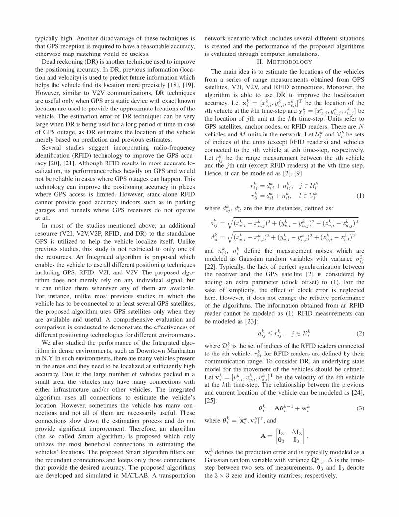
is evaluated. Fig. 1 shows the simulation results of the Inte-
grated algorithm. The localization error as a function of the
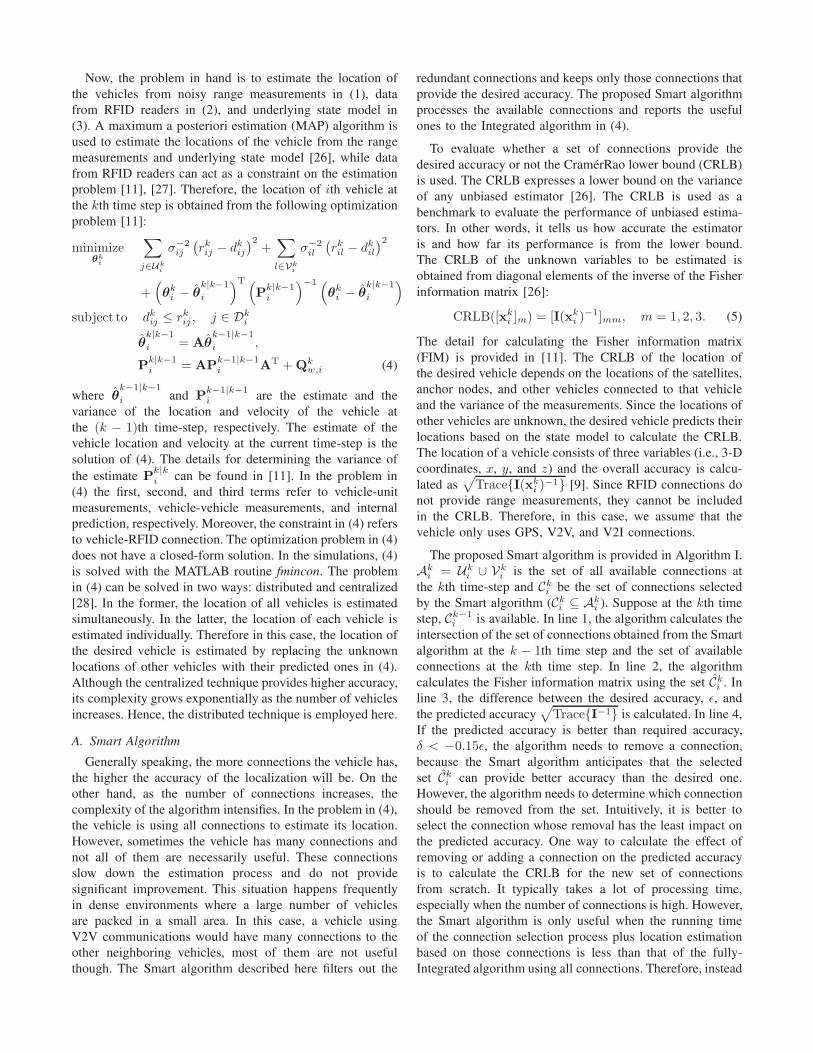
time-step for these cases is depicted in Fig. 1b. Fig. 1c shows
the cumulative distribution function (CDF) of the localization
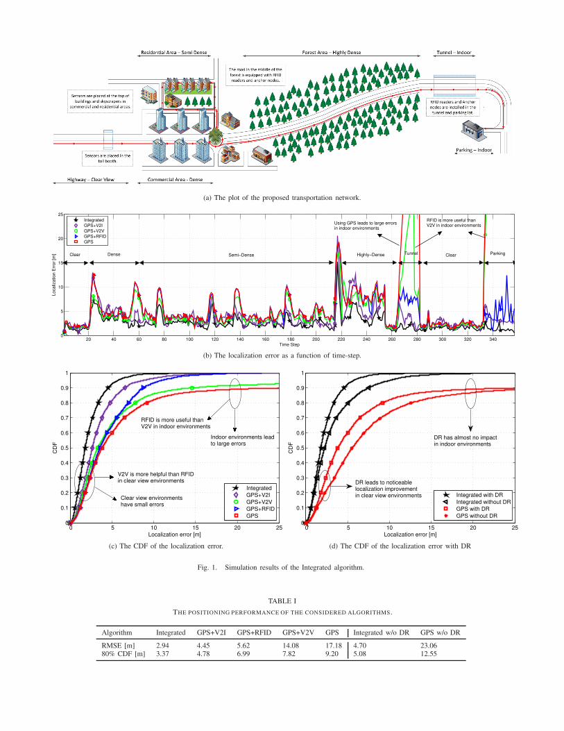
(a) The plot of the proposed transportation network.
20 40 60 80 100 120 140 160 180 200 220 240 260 280 300 320 3400
5
10
15
20
25
Time Step
Lo
ca
liza
tio
n E
rro
r [m
]
Integrated
GPS+V2I
GPS+V2V
GPS+RFID
GPS
Clear Dense Highly−Dense ParkingSemi−Dense Tunnel Clear
Using GPS leads to large errorsin indoor environments
RFID is more useful thanV2V in indoor environments
(b) The localization error as a function of time-step.
0 5 10 15 20 250
0.1
0.2
0.3
0.4
0.5
0.6
0.7
0.8
0.9
1
Localization error [m]
CD
F
Integrated
GPS+V2I
GPS+V2V
GPS+RFID
GPS
Indoor environments leadto large errors
RFID is more useful thanV2V in indoor environments
V2V is more helpful than RFIDin clear view environments
Clear view environmentshave small errors
(c) The CDF of the localization error.
0 5 10 15 20 250
0.1
0.2
0.3
0.4
0.5
0.6
0.7
0.8
0.9
1
Localization error [m]
CD
F
Integrated with DR
Integrated without DR
GPS with DR
GPS without DR
DR has almost no impactin indoor environments
DR leads to noticeablelocalization improvementin clear view environments
(d) The CDF of the localization error with DR
Fig. 1. Simulation results of the Integrated algorithm.
TABLE I
THE POSITIONING PERFORMANCE OF THE CONSIDERED ALGORITHMS.
Algorithm Integrated GPS+V2I GPS+RFID GPS+V2V GPS Integrated w/o DR GPS w/o DR
RMSE [m] 2.94 4.45 5.62 14.08 17.18 4.70 23.0680% CDF [m] 3.37 4.78 6.99 7.82 9.20 5.08 12.55
error for different cases. The performance of GPS is almost
satisfactory in all regions except for indoor (i.e., tunnel and
parking) and very dense (i.e., forest) environments. On the
other hand, the estimated location of the vehicle using the
Integrated algorithm provides remarkable performance in all
regions, especially in highly dense and indoor environments
where GPS reception is very weak. The reason is that the
integrated positioning exploits other resources which enhance
the positioning accuracy. As depicted in the GPS+RFID
curve, RFID technology can improve the location perfor-
mance, especially when the vehicle is inside the tunnel and
parking garage. However, in other regions where the GPS
reception is sufficient, RFID technology cannot help the
algorithm in terms of accuracy. The behavior of GPS+V2V
is almost opposite to GPS+RFID. In other words, V2V
technology can slightly help the vehicle in the clear view,
commercial and residential regions because it provides the
vehicle with more useful connections. However, V2V cannot
improve the performance in indoor regions considerably,
because in indoor environments V2V technology uses other
vehicles information which are also inside the tunnel (or
parking garage) and do not have enough connections due
to GPS outage and their location information is not as
reliable as other resources such as RFID and V2I. Among
GPS-aided techniques (RFID, V2V, and V2I), V2I provides
considerably better accuracy. The reason is that unlike RFID,
V2I is associated with the range measurement which is more
useful than presence detection for localization. V2I also has
more valuable information than V2V because the source
of information in V2I is an infrastructure with a fixed and
known location, while the source of information in V2V is
another vehicle whose location is not accurate.
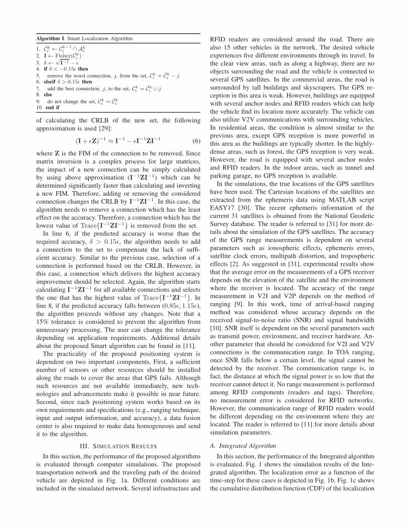
In all previous cases, the algorithms use the internal DR.
Evaluating the effect of the internal DR sensor, Fig. 1d
shows that using DR is highly beneficial for both Integrated
positioning and GPS positioning. However, DR is not useful
for GPS positioning when the vehicle is in indoor environ-
ments. In DR technique, the previous estimate is used to
predict the future vehicles locations. If no measurement is
available and if the vehicle changes its velocity frequently,
the prediction and the true location of the vehicle get farther
and farther apart which generates significantly large errors.
Therefore, using DR without having extra measurements
does not necessarily lead to performance improvement. This
conclusion is also clearly demonstrated in Fig. 1b where DR
is not useful anymore when the vehicle enters the tunnel and
parking garage, as DR predicts the wrong direction for the
vehicle in the absence of measurements.
In Table I, the performance of the considered algorithms
is summarized in terms of root-mean-square error (RMSE)
and 80% CDF. RMSE represents the difference between the
estimated location and the true one on average [11]. As can
be seen, the RMSE of the GPS is about 17 m, although
its localization error is less than 9.2 m about 80% of the
time. The reason is that the bad performance of GPS which
happens only 20% of the time has a great impact on the
average error represented by RMSE.
0 20 40 60 80 100 120 140 160 180 2000
20
40
60
80
100
120
140
160
180
200
x [m]
y [m
]
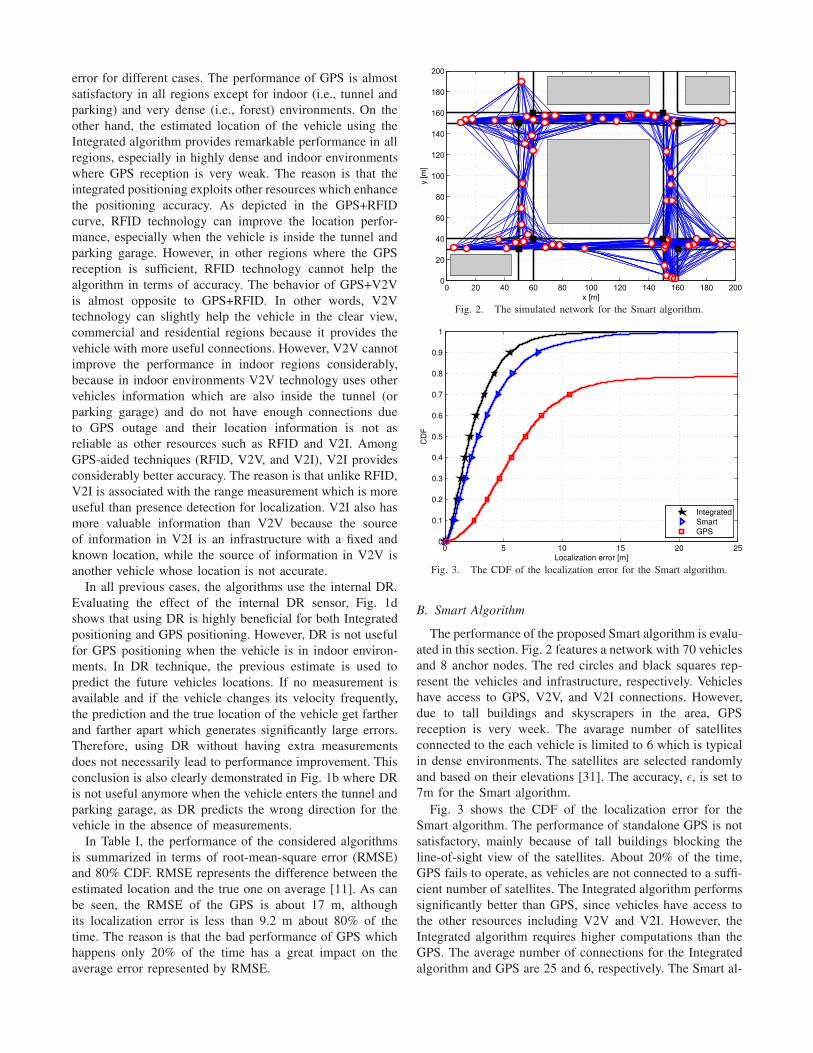
Fig. 2. The simulated network for the Smart algorithm.
0 5 10 15 20 250
0.1
0.2
0.3
0.4
0.5
0.6
0.7
0.8
0.9
1
Localization error [m]
CD
F
Integrated
Smart
GPS
Fig. 3. The CDF of the localization error for the Smart algorithm.
B. Smart Algorithm
The performance of the proposed Smart algorithm is evalu-
ated in this section. Fig. 2 features a network with 70 vehicles
and 8 anchor nodes. The red circles and black squares rep-
resent the vehicles and infrastructure, respectively. Vehicles
have access to GPS, V2V, and V2I connections. However,
due to tall buildings and skyscrapers in the area, GPS
reception is very week. The avarage number of satellites
connected to the each vehicle is limited to 6 which is typical
in dense environments. The satellites are selected randomly
and based on their elevations [31]. The accuracy, ǫ, is set to
7m for the Smart algorithm.
Fig. 3 shows the CDF of the localization error for the
Smart algorithm. The performance of standalone GPS is not
satisfactory, mainly because of tall buildings blocking the
line-of-sight view of the satellites. About 20% of the time,
GPS fails to operate, as vehicles are not connected to a suffi-
cient number of satellites. The Integrated algorithm performs
significantly better than GPS, since vehicles have access to
the other resources including V2V and V2I. However, the
Integrated algorithm requires higher computations than the
GPS. The average number of connections for the Integrated
algorithm and GPS are 25 and 6, respectively. The Smart al-
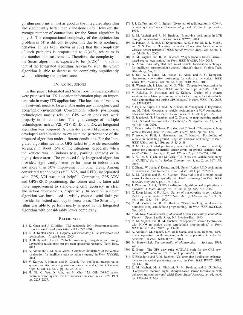
gorithm performs almost as good as the Integrated algorithm
and significantly better than standalone GPS. However, the
average number of connections for the Smart algorithm is
only 5. The computational complexity of the optimization
problem in (4) is difficult to determine due to its nonlinear
behavior. It has been shown in [32] that the complexity
of such problems is proportional to O(m3), where m is
the number of measurements. Therefore, the complexity of
the Smart algorithm is expected to be (5/25)3 = 0.8% of
that of the Integrated algorithm. As can be seen, the Smart
algorithm is able to decrease the complexity significantly
without affecting the performance.
IV. CONCLUSIONS
In this paper, Integrated and Smart positioning algorithms
were proposed for ITS. Location information plays an impor-
tant role in many ITS applications. The locations of vehicles
in a network needs to be available under any atmospheric and
geographic environment. Conventional vehicle positioning
technologies mostly rely on GPS which does not work
properly in all conditions. Taking advantage of multiple
technologies such as V2I, V2V, RFID, and DR, an Integrated
algorithm was proposed. A close-to-real-world scenario was
developed and simulated to evaluate the performance of the
proposed algorithm under different conditions. For the Inte-
grated algorithm scenario, GPS failed to provide reasonable
accuracy in about 15% of the situations, especially when
the vehicle was in indoors (e.g., parking garages) or in
highly-dense areas. The proposed fully Integrated algorithm
provided significantly better performance in indoor areas
and more than 50% improvement in other areas. Among
considered technologies (V2I, V2V, and RFID) incorporated
with GPS, V2I was most helpful. Comparing GPS+V2V
and GPS+RFID positioning, the former and the latter add
more improvement to stand-alone GPS accuracy in clear
and indoor environments, respectively. In addition, a Smart
algorithm was introduced to wisely choose useful links yet
provide the desired accuracy in dense areas. The Smart algo-
rithm was able to perform nearly as good as the Integrated
algorithm with considerably lower complexity.
REFERENCES
[1] K. Chen and J. C. Miles, “ITS handbook 2004: Recommendationsfrom the world road association (PIARC),” 2004.
[2] E. D. Kaplan and C. J. Hegarty, Understanding GPS: principles and
applications. Artech house, 2005.
[3] D. Bevly and J. Farrell, “Vehicle positioning, navigation, and timing:Leveraging results from ear program-sponsored research,” Tech. Rep.,2013.
[4] A. Amini and J. M. de la Garza, “Computer simulations of the vehiclelocalization for intelligent transportation systems,” in Proc. ICCCBE,2014.
[5] V. Katiyar, P. Kumar, and N. Chand, “An intelligent transportationsystems architecture using wireless sensor networks,” Int. J. Comput.
Appl. T., vol. 14, no. 2, pp. 22–26, 2011.
[6] H. Oh, C. Yae, D. Ahn, and H. Cho, “5.8 GHz DSRC packetcommunication system for ITS services,” in Proc. IEEE VTS, 1999,pp. 2223–2227.
[7] J. J. Caffery and G. L. Stuber, “Overview of radiolocation in CDMAcellular systems,” IEEE Commun. Mag., vol. 36, no. 4, pp. 38–45,1998.
[8] R. M. Vaghefi and R. M. Buehrer, “Improving positioning in LTEthrough collaboration,” in Proc. IEEE WPNC, 2014.
[9] N. Patwari, J. N. Ash, S. Kyperountas, A. O. Hero III, R. L. Moses,and N. S. Correal, “Locating the nodes: Cooperative localization inwireless sensor networks,” IEEE Signal Process. Mag., vol. 22, no. 4,pp. 54–69, Jul. 2005.
[10] R. M. Vaghefi and R. M. Buehrer, “Asynchronous time-of-arrival-based source localization,” in Proc. IEEE ICASSP, May 2013.
[11] A. Amini, “An integrated and smart vehicle localization techniquefor intelligent transportation systems,” Master’s thesis, Virginia Tech,Blacksburg, VA, 2013.
[12] J. Yao, A. T. Balaei, M. Hassan, N. Alam, and A. G. Dempster,“Improving cooperative positioning for vehicular networks,” IEEE
Trans. Veh. Technol., vol. 60, no. 6, pp. 2810–2823, 2011.[13] H. Wymeersch, J. Lien, and M. Z. Win, “Cooperative localization in
wireless networks,” Proc. IEEE, vol. 97, no. 2, pp. 427–450, 2009.[14] V. Kukshya, H. Krishnan, and C. Kellum, “Design of a system
solution for relative positioning of vehicles using vehicle-to-vehicleradio communications during GPS outages,” in Proc. IEEE VTC, 2005,pp. 1313–1317.
[15] S. Fujii, A. Fujita, T. Umedu, S. Kaneda, H. Yamaguchi, T. Higashino,and M. Takai, “Cooperative vehicle positioning via V2V communica-tions and onboard sensors,” in Proc. IEEE VTC, 2011, pp. 1–5.
[16] G. Jagadeesh, T. Srikanthan, and X. Zhang, “A map matching methodfor GPS based real-time vehicle location,” J. Navigation, vol. 57, no. 3,pp. 429–440, 2004.
[17] S. Brakatsoulas, D. Pfoser, R. Salas, and C. Wenk, “On map-matchingvehicle tracking data,” in Proc. Intl. VLDB, 2005, pp. 853–864.
[18] T. Aono, K. Fujii, S. Hatsumoto, and T. Kamiya, “Positioning ofvehicle on undulating ground using GPS and dead reckoning,” in Proc.
IEEE ICRA, vol. 4, 1998, pp. 3443–3448.[19] D. M. Bevly, “Global positioning system (GPS): A low-cost velocity
sensor for correcting inertial sensor errors on ground vehicles: Sen-sors,” ASME J. Dyn. Syst. T., vol. 126, no. 2, pp. 255–264, 2004.
[20] E.-K. Lee, S. Y. Oh, and M. Gerla, “RFID assisted vehicle positioningin VANETs,” Pervasive Mobile Comput., vol. 8, no. 2, pp. 167–179,2012.
[21] E. Zhang, W. Jiang, Y. Kuang, and M. Umer, “Active RFID positioningof vehicles in road traffic,” in Proc. ISCIT, 2011, pp. 222–227.
[22] R. M. Vaghefi and R. M. Buehrer, “Received signal strength-basedsensor localization in spatially correlated shadowing,” in Proc. IEEE
ICASSP, May 2013, pp. 4076–4080.[23] J. Zhou and J. Shi, “RFID localization algorithms and applications -
a review,” J. Intell. Manuf., vol. 20, no. 6, pp. 695–707, 2009.[24] X. Rong Li and V. P. Jilkov, “Survey of maneuvering target tracking.
Part I. dynamic models,” IEEE Trans. Aerosp. Electron. Syst., vol. 39,no. 4, pp. 1333–1364, 2003.
[25] R. M. Vaghefi and R. M. Buehrer, “Target tracking in nlos envi-ronments using semidefinite programming,” in Proc. IEEE MILCOM,Nov. 2013.
[26] S. M. Kay, Fundamentals of Statistical Signal Processing: Estimation
Theory. Upper Saddle River, NJ: Prentice-Hall, 1993.[27] R. M. Vaghefi and R. M. Buehrer, “Cooperative sensor localization
with NLOS mitigation using semidefinite programming,” in Proc.
IEEE WPNC, Mar. 2012, pp. 13–18.[28] A. Amini, R. M. Vaghefi, J. M. de la Garza, and R. M. Buehrer, “GPS-
free cooperative mobile tracking with the application in vehicularnetworks,” in Proc. IEEE WPNC, 2014.
[29] M. Hazewinkel, Encyclopaedia of Mathematics. Springer, 1993,vol. 9.
[30] K. Borre, “The GPS easy suite–MATLAB code for the GPS new-comer,” GPS Solutions, vol. 7, no. 1, pp. 47–51, 2003.
[31] Z. Biskaduros and R. M. Buehrer, “Collaborative localization enhance-ment to the global positioning system,” in Proc. IEEE WPNC, 2012,pp. 142–146.
[32] R. M. Vaghefi, M. R. Gholami, R. M. Buehrer, and E. G. Strom,“Cooperative received signal strength-based sensor localization withunknown transmit powers,” IEEE Trans. Signal Process., vol. 61, no. 6,pp. 1389–1403, Mar. 2013.


