

University of Illinois at Urbana-Champaign • Metals Processing Simulation Lab • Lifeng Zhang (2001)
Inclusion Entrapment Literature Review and Modeling
Inclusion Entrapment Literature Review and Modeling
Lifeng Zhang
Department of Mechanical &. Industrial EngineeringUniversity of Illinois at Urbana-Champaign
October 18, 2001
Lifeng Zhang
Department of Mechanical &. Industrial EngineeringUniversity of Illinois at Urbana-Champaign
October 18, 2001
University of Illinois at Urbana-Champaign • Metals Processing Simulation Lab • Lifeng Zhang (2001)
Acknowledgements
The authors would like to thank:
l Accmold
l AK Steel
l Allegheny Ludlum Steel
l Columbus Stainless Steel
l LTV Steel
l Hatch Associates
l Stollberg, Inc.
l National Science Foundation
l National Center for the Supercomputing Applications (NCSA)
l Continuous Casting Consortium (CCC) at UIUC
The authors would like to thank:
l Accmold
l AK Steel
l Allegheny Ludlum Steel
l Columbus Stainless Steel
l LTV Steel
l Hatch Associates
l Stollberg, Inc.
l National Science Foundation
l National Center for the Supercomputing Applications (NCSA)
l Continuous Casting Consortium (CCC) at UIUC
University of Illinois at Urbana-Champaign • Metals Processing Simulation Lab • Lifeng Zhang (2001)
Fluid Flow and Inclusions Behavior in Steel Caster=
Velocity, Turbulence Energy and Its Dissipation Rate for a Full-Developed Pipe Flow
=
Pressure and Level Fluctuation of Top Surface of Mold=
Fluid Flow and Particle Behavior in 1:1 Mold Water Model=
Background — Review of Inclusions in Steel=
ContentsContents

University of Illinois at Urbana-Champaign • Metals Processing Simulation Lab • Lifeng Zhang (2001)
Background — Review of Inclusions in Steel
Background — Review of Inclusions in Steel

University of Illinois at Urbana-Champaign • Metals Processing Simulation Lab • Lifeng Zhang (2001)
Phenomena
EvolutionMechanisms:
Processes
Steps of Inclusions Nucleation, Precipitation, Growth and Removal from Liquid Metals
log (time)
Time for nucleation start
top slag and refractory walls
Nucleation, Precipitation, andgrowth of particles
Particle growth by coagulation or agglomeration
Particle removal
“Stable suspension“of inclusions in liquid steel
Inclusion removal by-diffusion deoxidation- Interfacial reactions
Simultaneous events in Vessel
1. Elements Diffusion ([O], [Al], or [Si]) (Ostwald- Ripening)
2. Brownian collision
Collision between particles (Brownian, Stokes, and turbulence collision)
Rising by buoyancy,bubble flotation and flow transport
t=0, Adding of deoxidizer
Time for collisions todominate size evolution
Melting and Mixing of Deoxidizer

University of Illinois at Urbana-Champaign • Metals Processing Simulation Lab • Lifeng Zhang (2001)
Evolution Mechnisms Related to Particle Size
log time
Independent of fluid flow Dependent on fluid flow in Ladles, Tundish and Mold
Nucleation
Particle growing
Particle removal
0 t‘‘‘‘(rP>25µm)
Ostwald-Ripening (Elements Diffusion)
Brownian collision
Turbulent collision
Stokes collision (no flow)
t‘(rP>0.1µm)
t‘‘‘(rP>14µm)
t‘‘ (rP>1µm)

University of Illinois at Urbana-Champaign • Metals Processing Simulation Lab • Lifeng Zhang (2001)
Steel Cleanliness ⇔ Inclusions in Steel Steel Cleanliness ⇔ Inclusions in Steel SizeShapeSizeShape
l Direct Measurement of Inclusions:
Ù Metallographical microscope observation
(two dimensional slices)
Ù Slime (time consuming)
Ù Others (Cone machining, laser, electrical, ultrasonic, sulfur print)
l Indirect Methods
Ù Total Oxygen (T.O.) measurement
Ù Nitrogen Pickup
Ù Dissolved Al loss for LCAK Steel
Ù Analysis of slag composition evolution
Evaluation Methods of Steel CleanlinessEvaluation Methods of Steel Cleanliness
w Sampling difficulties
w Time consuming
w Sampling difficulties
w Time consuming

University of Illinois at Urbana-Champaign • Metals Processing Simulation Lab • Lifeng Zhang (2001)
Inclusions in Tunidsh Steel Samples Showing Liquid Slag
Inclusions in Tunidsh Steel Samples Showing Liquid Slag
Steel grade: LCAK SteelSource: Slime test ResidualTypical composition: Al2O3 24%, SiO2 29%, MnO 20%, FeO 16%
CaO 4%, MgO 1.4%, others 4.6%
Steel grade: LCAK SteelSource: Slime test ResidualTypical composition: Al2O3 24%, SiO2 29%, MnO 20%, FeO 16%
CaO 4%, MgO 1.4%, others 4.6%

University of Illinois at Urbana-Champaign • Metals Processing Simulation Lab • Lifeng Zhang (2001)
Steel grade: LCAK SteelSource: Slime test ResidualTypical composition: Al2O3 96.2%, SiO2 2.3%, MnO 1.3%, FeO 0.2%
Steel grade: LCAK SteelSource: Slime test ResidualTypical composition: Al2O3 96.2%, SiO2 2.3%, MnO 1.3%, FeO 0.2%
Alumina Inclusions in Continuous Casting SlabAlumina Inclusions in Continuous Casting Slab

University of Illinois at Urbana-Champaign • Metals Processing Simulation Lab • Lifeng Zhang (2001)
Alumina Clusters in Carbon Steel[1]Alumina Clusters in Carbon Steel[1]
[1] R.Rastogi and A. W. Cramb. Inclusions Formation and Agglomeration in Aluminum Killed Steels. 84th Steelmaking Conference Proceedings, ISS, Warrendale, PA, USA, P789-829
[1] R.Rastogi and A. W. Cramb. Inclusions Formation and Agglomeration in Aluminum Killed Steels. 84th Steelmaking Conference Proceedings, ISS, Warrendale, PA, USA, P789-829

University of Illinois at Urbana-Champaign • Metals Processing Simulation Lab • Lifeng Zhang (2001)
25 30 35 40 45 50 55 60 650
1
2
3
4
[1]
Sliv
er In
dex
T.O (ppm)
0 5 10 15 20 25 3060
80
100
120
140
160
180
200
220
240
From ladle to mold [2] From ladle to tundish [3]
Al l
oss
(ppm
)
%FeO in ladle slag (%)
[4][4]
Example of Total Oxygen, Al loss, Nitrogen PickupExample of Total Oxygen, Al loss, Nitrogen Pickup
[1] Bonila C. et al. 78th Steelmaking Conference Proceedings, Vol.78, 1995, p629-635[2] Chakraborty S. et al. 77th Steelmaking Conference Proceedings, Vol.77, 1994, p389-395[3] Ahlborg K. V. et al. 76th Steelmaking Conference Proceedings, Vol.76, 1993, p469-473[4] Melville S. D. et al. 78th Steelmaking Conference Proceedings, Vol.78, 1995, p563-569
[1] Bonila C. et al. 78th Steelmaking Conference Proceedings, Vol.78, 1995, p629-635[2] Chakraborty S. et al. 77th Steelmaking Conference Proceedings, Vol.77, 1994, p389-395[3] Ahlborg K. V. et al. 76th Steelmaking Conference Proceedings, Vol.76, 1993, p469-473[4] Melville S. D. et al. 78th Steelmaking Conference Proceedings, Vol.78, 1995, p563-569

University of Illinois at Urbana-Champaign • Metals Processing Simulation Lab • Lifeng Zhang (2001)
Al2O3 Inclusion Absorption to Mold FluxAl2O3 Inclusion Absorption to Mold Flux
0 20 40 60 80 100 120 140 160 1803
4
5
6
7
8
Experiment at Baosteel (1992)LCAK Steel250ton ladle60ton tundishcasting speed 1.1m/minslab section: 250mmX1300mm
Al 2O
3 in
mol
d flu
x (
%)
casting time (min)

University of Illinois at Urbana-Champaign • Metals Processing Simulation Lab • Lifeng Zhang (2001)
Inclusion Phenomena in Continuous Casting MoldInclusion Phenomena in Continuous Casting Mold
Inclusion Sources:=Carrying in through nozzleÙ Deoxidation ProductsÙ Nozzle clogÙ Entrainment of tundish/ladle slag (reoxidation by SiO2, FeO, MnO in slag)
=Entrainment of mold slag by excessive top surface level fluctuation =Reoxidation by air absorption from nozzle leaks
=Argon bubbles
=Precipitation of inclusion in low superheat, such as TiO2
Inclusion Removal:= Buoyancy rising = Fluid flow transport= Attachment to bubble surface and fast rising (Bubble flotation)= Inclusion growth by collision and Ostwald-Ripening= Absorption from steel to slag at interface
Inclusion Destination:= Top slag layer (safe removal)= Trapped in solidification shell (defect)

University of Illinois at Urbana-Champaign • Metals Processing Simulation Lab • Lifeng Zhang (2001)
All inclusions phenomena in mold are greatly affected by bulk fluid flow pattern, thus it is important to study the fluid flow in mold.
All inclusions phenomena in mold are greatly affected by bulk fluid flow pattern, thus it is important to study the fluid flow in mold.
Conclusion Conclusion

University of Illinois at Urbana-Champaign • Metals Processing Simulation Lab • Lifeng Zhang (2001)
1. Large Eddy Simulation (LES)Ù Random Walk Model for Particle Motion
2. Reynolds Stress Model (RSM)Ù Random Walk Model for Particle Motion
3. k-ε Model for Fluid FlowÙ Random Walk Model for Particle Motion Ù Streamline Model for Particle Motion
4. k-ε Model for Top Surface Pressure and Level Fluctuation
Cases of Fluid Flow and Inclusion Motion Simulation in the Current Report
Cases of Fluid Flow and Inclusion Motion Simulation in the Current Report
Water Model:Water Model:
Steel Caster:Steel Caster:
1. k-ε Model for Fluid Flow
Ù Four Cases for Inclusion Motion by Random Walk Model
1. k-ε Model for Fluid Flow
Ù Four Cases for Inclusion Motion by Random Walk Model

University of Illinois at Urbana-Champaign • Metals Processing Simulation Lab • Lifeng Zhang (2001)
Fluid Flow and Particle Behavior in 1:1 Water Model
Fluid Flow and Particle Behavior in 1:1 Water Model
University of Illinois at Urbana-Champaign • Metals Processing Simulation Lab • Lifeng Zhang (2001)
25o down inflowV=1.69m/s
Inlet Port
AA'
A-A'
(a) (b)
Symmetryplane
Free Slip
Outlet Port51mm
56mm
2.152m
0.238m 0.965m
Outflow
Inlet Jet: 25o down
Water
0.150m
x z
y
Widefaces
Narrowfaces
Submerged entry nozzle
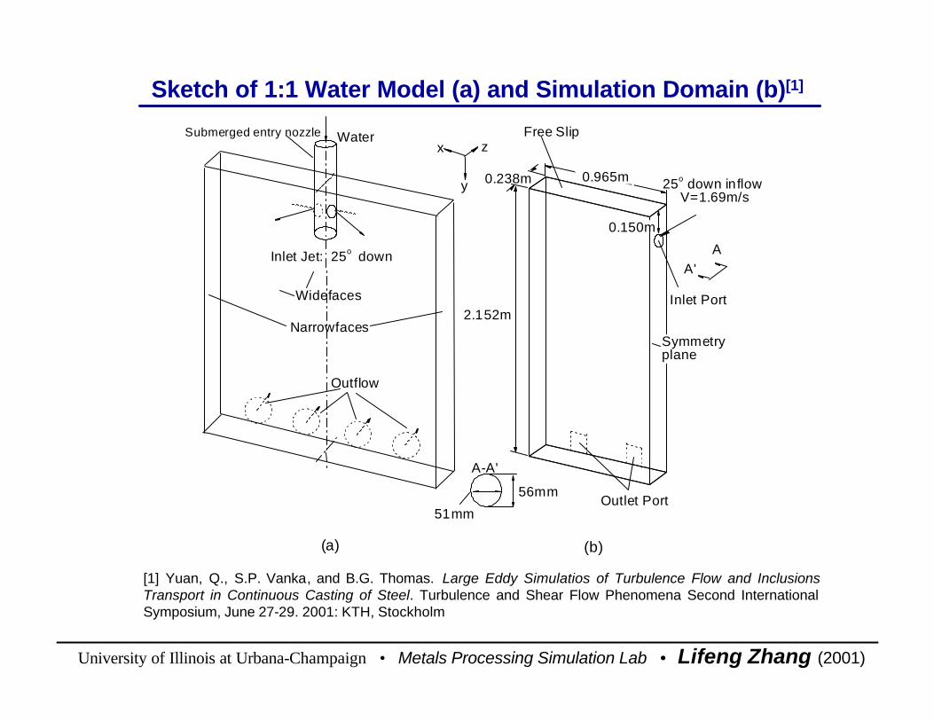
Sketch of 1:1 Water Model (a) and Simulation Domain (b)[1]Sketch of 1:1 Water Model (a) and Simulation Domain (b)[1]
[1] Yuan, Q., S.P. Vanka, and B.G. Thomas. Large Eddy Simulatios of Turbulence Flow and Inclusions Transport in Continuous Casting of Steel. Turbulence and Shear Flow Phenomena Second International Symposium, June 27-29. 2001: KTH, Stockholm
[1] Yuan, Q., S.P. Vanka, and B.G. Thomas. Large Eddy Simulatios of Turbulence Flow and Inclusions Transport in Continuous Casting of Steel. Turbulence and Shear Flow Phenomena Second International Symposium, June 27-29. 2001: KTH, Stockholm

University of Illinois at Urbana-Champaign • Metals Processing Simulation Lab • Lifeng Zhang (2001)
300Corresponding alumina inclusion diameter in steel caster (µm)
LES pipe simulation results[1]Inlet condition
988Particle density (kg/m3)
3.8 2-3Particle size (diameter) (mm)
1.0 ×10⁻⁶Fluid kinetic viscosity (m2/s)
1000Fluid density (kg/m3)
0.0152Casting speed (m/s)
0.00344Average inlet flow rate (m3/s)
0.238Mold/Domain thickness (m)
1.83Mold/Domain width (m)
2.152Mold/Domain height (m)
0.150Submergence depth (m)
25oInlet jet angle
25oNozzle angle
0.051×0.056Nozzle port size/ Inlet port size (x×y) (m)
SimulationExperiment
Experimental and Simulation ParametersExperimental and Simulation Parameters
[1] Yuan, Q., S.P. Vanka, and B.G. Thomas. Large Eddy Simulatios of Turbulence Flow and Inclusions Transport in Continuous Casting of Steel. Turbulence and Shear Flow Phenomena Second International Symposium, June 27-29. 2001: KTH, Stockholm
[1] Yuan, Q., S.P. Vanka, and B.G. Thomas. Large Eddy Simulatios of Turbulence Flow and Inclusions Transport in Continuous Casting of Steel. Turbulence and Shear Flow Phenomena Second International Symposium, June 27-29. 2001: KTH, Stockholm

University of Illinois at Urbana-Champaign • Metals Processing Simulation Lab • Lifeng Zhang (2001)
Mesh for k-ε and RSM Water Model SimulationsMesh for k-ε and RSM Water Model Simulationsxx
yy
zz
NX=40
NY=86
NZ=34
Total Nodes: 116,960
NX=40
NY=86
NZ=34
Total Nodes: 116,960

University of Illinois at Urbana-Champaign • Metals Processing Simulation Lab • Lifeng Zhang (2001)
Non-Uniform Inlet Condition (LES Skewed Pipe Flow Simulation)[1]Non-Uniform Inlet Condition (LES Skewed Pipe Flow Simulation)[1]
Z
Y
2 .3 22 .1 6
2 .0 11 .8 5
1 .7 01 .5 41 .3 9
1 .2 31 .0 8
0 .9 30 .7 7
0 .6 20 .4 6
0 .3 10 .1 5
x-velocity (m/s)
Z
Y
-0 .07
-0 .14-0 .21
-0 .28
-0 .35-0 .42
-0 .49
-0 .56-0 .63
-0 .70
-0 .77-0 .84
-0 .91-0 .98
-1 .05
y-velocity (m/s)
Y
Z
13.7212.8111.9010.9910.08
9.178.267.356.445.534.623.712.802.301.891.501.201.000.980.80
Turbulent energydissipation rate (m2/s3)
YZ
0.360.340.320.290.270.250.220.210.200.180.150.130.120.110.080.060.04
Turbulent energy (m2/s2)
[1] Yuan, Q., S.P. Vanka, and B.G. Thomas. Large Eddy Simulatios of Turbulence Flow and Inclusions Transport in Continuous Casting of Steel. Turbulence and Shear Flow Phenomena Second International Symposium, June 27-29. 2001: KTH, Stockholm
[1] Yuan, Q., S.P. Vanka, and B.G. Thomas. Large Eddy Simulatios of Turbulence Flow and Inclusions Transport in Continuous Casting of Steel. Turbulence and Shear Flow Phenomena Second International Symposium, June 27-29. 2001: KTH, Stockholm

University of Illinois at Urbana-Champaign • Metals Processing Simulation Lab • Lifeng Zhang (2001)
up,i , the particle velocity at i direction;xp,i , the particle position at i direction; µ is the fluids viscosity; ρp , ρ , the particle density and fluid density respectively; Rep,, the particle Reynolds number;CD , the drag force coefficient;
g, is the gravitational acceleration; aother,i , the other forces’ acceleration, which is ignored in the present study.
( ) ( )iother
P
PxiPi
PP
PDpi aguud
Cdt
du,2
Re43
+−
+−=ρ
ρρρ
µdt
dxu ip
ip.
, =
Particle Motion EquationsParticle Motion Equations
( )653.0Re186.01Re24
pp
DC +=
Boundary condition for particles:
Escape from top surface and outlet, reflect from other faces (no entrapment to solidified shell)
Boundary condition for particles:
Escape from top surface and outlet, reflect from other faces (no entrapment to solidified shell)
University of Illinois at Urbana-Champaign • Metals Processing Simulation Lab • Lifeng Zhang (2001)
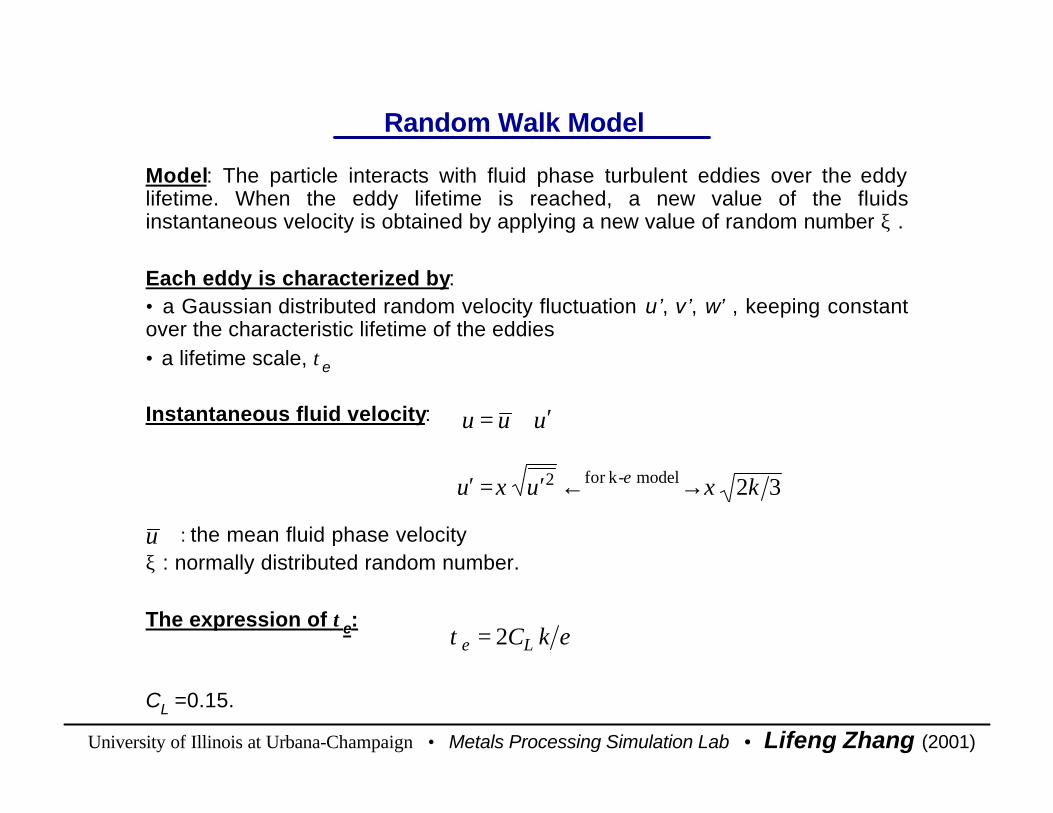
Model: The particle interacts with fluid phase turbulent eddies over the eddy lifetime. When the eddy lifetime is reached, a new value of the fluids instantaneous velocity is obtained by applying a new value of random number ξ .
Each eddy is characterized by:• a Gaussian distributed random velocity fluctuation u’, v’, w’ , keeping constant over the characteristic lifetime of the eddies • a lifetime scale, τe
Instantaneous fluid velocity:
Random Walk ModelRandom Walk Model
: the mean fluid phase velocityξ : normally distributed random number.
The expression of τe:
CL =0.15.
: the mean fluid phase velocityξ : normally distributed random number.
The expression of τe:
CL =0.15.
uuu ′+=
32model -kfor 2 kuu ξξ ε →←′=′
u
ετ kCLe 2=
University of Illinois at Urbana-Champaign • Metals Processing Simulation Lab • Lifeng Zhang (2001)
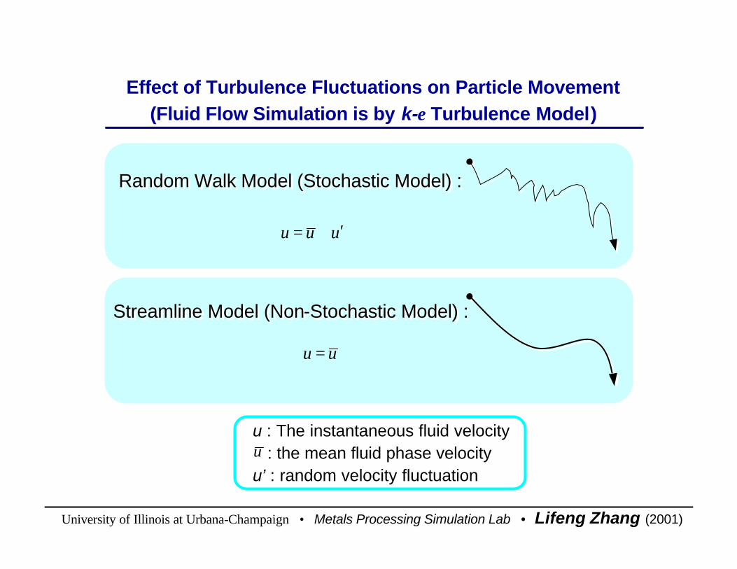
Effect of Turbulence Fluctuations on Particle Movement(Fluid Flow Simulation is by k-ε Turbulence Model)
Effect of Turbulence Fluctuations on Particle Movement(Fluid Flow Simulation is by k-ε Turbulence Model)
uuu ′+=
Random Walk Model (Stochastic Model) : Random Walk Model (Stochastic Model) :
uu =
Streamline Model (Non-Stochastic Model) : Streamline Model (Non-Stochastic Model) :
u : The instantaneous fluid velocity : the mean fluid phase velocity
u’ : random velocity fluctuation
u : The instantaneous fluid velocity : the mean fluid phase velocity
u’ : random velocity fluctuationu
University of Illinois at Urbana-Champaign • Metals Processing Simulation Lab • Lifeng Zhang (2001)
0.09 0.1 0.11 0.12 0.13 0.14 0.15
0.15
0.16
0.17
0.18
0.19
0.2
0.21
cast direction
Thickness of the narrow face
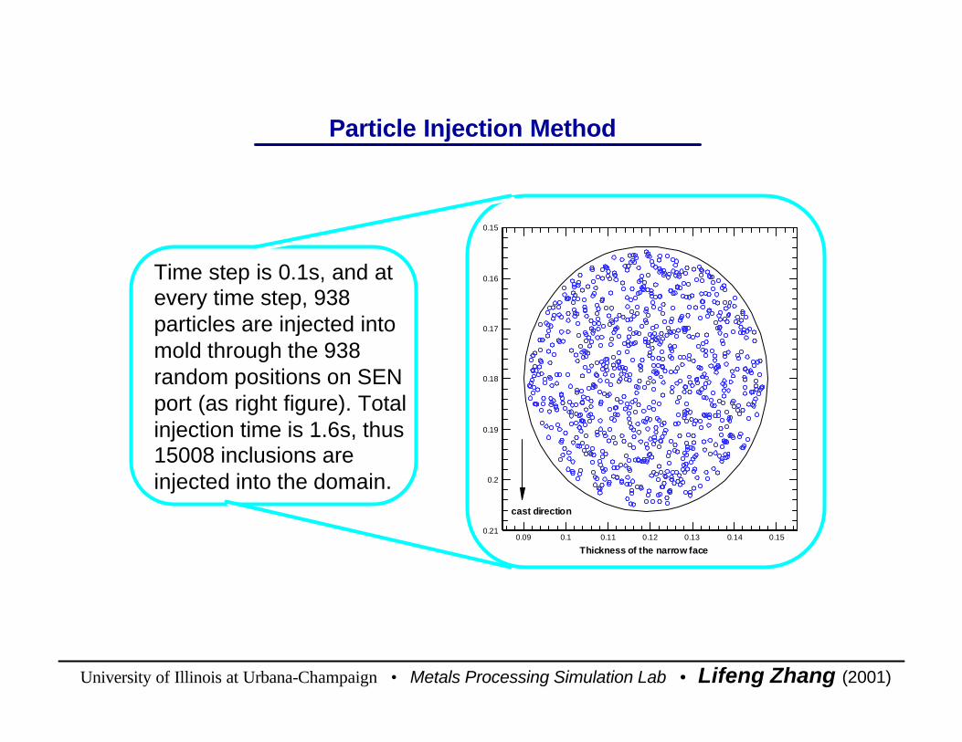
Particle Injection MethodParticle Injection Method
Time step is 0.1s, and at every time step, 938 particles are injected into mold through the 938 random positions on SEN port (as right figure). Total injection time is 1.6s, thus 15008 inclusions are injected into the domain.
Time step is 0.1s, and at every time step, 938 particles are injected into mold through the 938 random positions on SEN port (as right figure). Total injection time is 1.6s, thus 15008 inclusions are injected into the domain.
University of Illinois at Urbana-Champaign • Metals Processing Simulation Lab • Lifeng Zhang (2001)
0
0.2
0.4
0.6
0.8
1
1.2
1.4
1.6
1.8
2
0 0.20 0.2 0.4 0.6 0.8
0
0.2
0.4
0.6
0.8
1
1.2
1.4
1.6
1.8
2
0 0.2 0.4 0.6 0.8
0
0.2
0.4
0.6
0.8
1
1.2
1.4
1.6
1.8
2
0
0.2
0.4
0.6
0.8
1
1.2
1.4
1.6
1.8
2
0 0.2
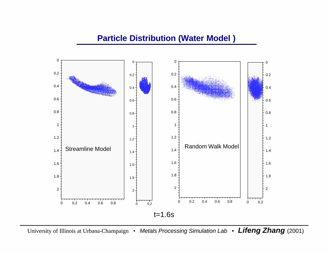
Streamline ModelStreamline Model Random Walk ModelRandom Walk Model
t=1.6s t=1.6s
Particle Distribution (Water Model )Particle Distribution (Water Model )
University of Illinois at Urbana-Champaign • Metals Processing Simulation Lab • Lifeng Zhang (2001)
0 0.2
0
0.2
0.4
0.6
0.8
1
1.2
1.4
1.6
1.8
2
0 0.2 0.4 0.6 0.8
0
0.2
0.4
0.6
0.8
1
1.2
1.4
1.6
1.8
2
0 0.2 0.4 0.6 0.8
0
0.2
0.4
0.6
0.8
1
1.2
1.4
1.6
1.8
2
0 0.2
0
0.2
0.4
0.6
0.8
1
1.2
1.4
1.6
1.8
2
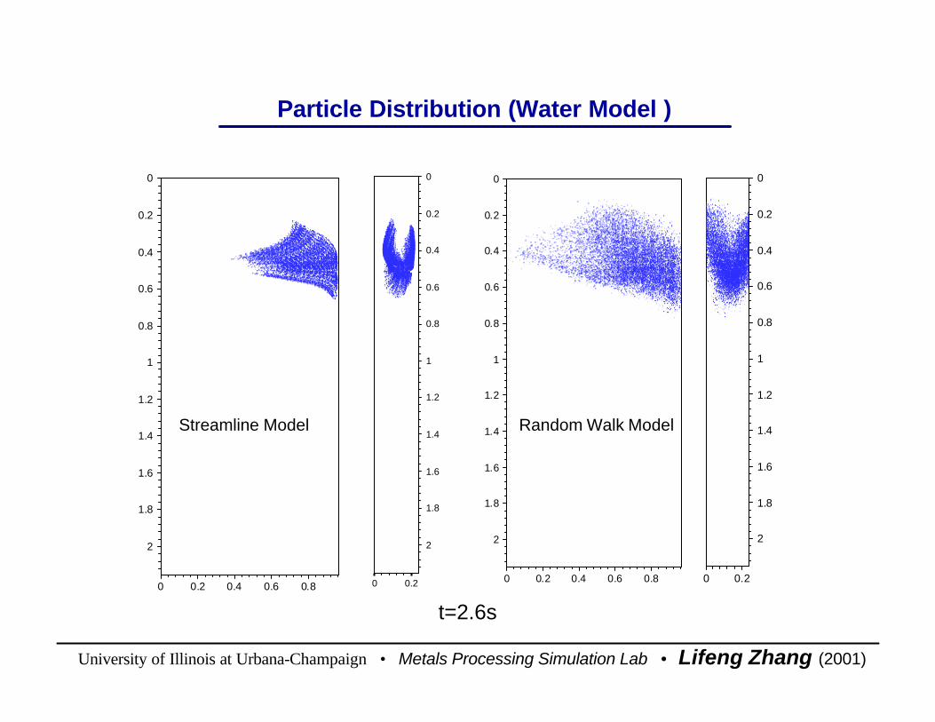
t=2.6s t=2.6s
Streamline ModelStreamline Model Random Walk ModelRandom Walk Model
Particle Distribution (Water Model )Particle Distribution (Water Model )

University of Illinois at Urbana-Champaign • Metals Processing Simulation Lab • Lifeng Zhang (2001)
0 0.2 0.4 0.6 0.8
0
0.2
0.4
0.6
0.8
1
1.2
1.4
1.6
1.8
2
0 0.2
0
0.2
0.4
0.6
0.8
1
1.2
1.4
1.6
1.8
2
0 0.2 0.4 0.6 0.8
0
0.2
0.4
0.6
0.8
1
1.2
1.4
1.6
1.8
2
0 0.2
0
0.2
0.4
0.6
0.8
1
1.2
1.4
1.6
1.8
2
t=10s t=10s
Streamline ModelStreamline Model Random Walk ModelRandom Walk Model
Particle Distribution (Water Model )Particle Distribution (Water Model )
University of Illinois at Urbana-Champaign • Metals Processing Simulation Lab • Lifeng Zhang (2001)
0 0.2 0.4 0.6 0.8
0
0.2
0.4
0.6
0.8
1
1.2
1.4
1.6
1.8
2
0 0.2
0
0.2
0.4
0.6
0.8
1
1.2
1.4
1.6
1.8
2
0 0.2 0.4 0.6 0.8
0
0.2
0.4
0.6
0.8
1
1.2
1.4
1.6
1.8
2
0
0.2
0.4
0.6
0.8
1
1.2
1.4
1.6
1.8
2
0 0.2
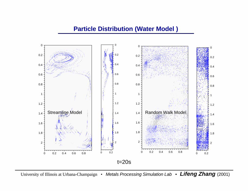
t=20s t=20s
Streamline ModelStreamline Model Random Walk ModelRandom Walk Model
Particle Distribution (Water Model )Particle Distribution (Water Model )

University of Illinois at Urbana-Champaign • Metals Processing Simulation Lab • Lifeng Zhang (2001)
0 0.2
0
0.2
0.4
0.6
0.8
1
1.2
1.4
1.6
1.8
2
0 0.2 0.4 0.6 0.8
0
0.2
0.4
0.6
0.8
1
1.2
1.4
1.6
1.8
2
0 0.2
0
0.2
0.4
0.6
0.8
1
1.2
1.4
1.6
1.8
2
0
0.2
0.4
0.6
0.8
1
1.2
1.4
1.6
1.8
2
0 0.2 0.4 0.6 0.8
t=30s t=30s
Streamline ModelStreamline Model Random Walk ModelRandom Walk Model
Particle Distribution (Water Model )Particle Distribution (Water Model )
University of Illinois at Urbana-Champaign • Metals Processing Simulation Lab • Lifeng Zhang (2001)
0 0.2 0.4 0.6 0.8
0
0.2
0.4
0.6
0.8
1
1.2
1.4
1.6
1.8
2
0 0.2
0
0.2
0.4
0.6
0.8
1
1.2
1.4
1.6
1.8
2
0 0.2
0
0.2
0.4
0.6
0.8
1
1.2
1.4
1.6
1.8
2
0 0.2 0.4 0.6 0.8
0
0.2
0.4
0.6
0.8
1
1.2
1.4
1.6
1.8
2
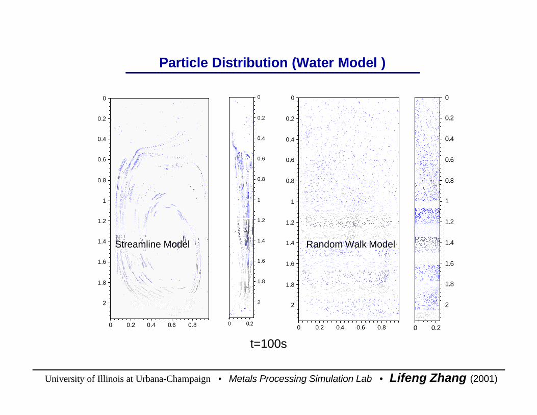
t=100s t=100s
Streamline ModelStreamline Model Random Walk ModelRandom Walk Model
Particle Distribution (Water Model )Particle Distribution (Water Model )

University of Illinois at Urbana-Champaign • Metals Processing Simulation Lab • Lifeng Zhang (2001)
Particle Velocities DistributionParticle Velocities Distribution
t=1.6s t=1.6s Streamline ModelStreamline ModelRandom Walk ModelRandom Walk Model
0.37890.33680.29470.25260.21050.16840.12630.08420.04210.0000
0.25m/s
Speed (m/s)
0.37890.33680.29470.25260.21050.16840.12630.08420.04210.0000
0.25m/s
Speed (m/s
University of Illinois at Urbana-Champaign • Metals Processing Simulation Lab • Lifeng Zhang (2001)
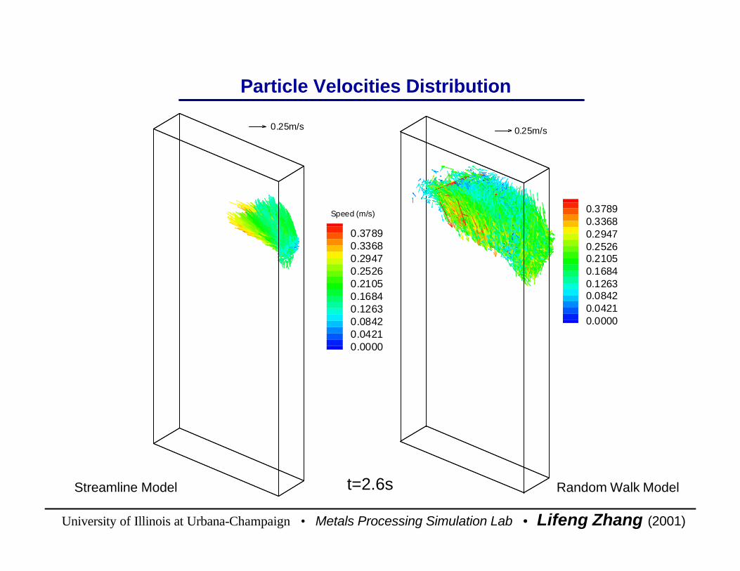
t=2.6s t=2.6s Streamline ModelStreamline Model Random Walk ModelRandom Walk Model
Particle Velocities DistributionParticle Velocities Distribution
0.37890.33680.29470.25260.21050.16840.12630.08420.04210.0000
0.25m/s
Speed (m/s) 0.37890.33680.29470.25260.21050.16840.12630.08420.04210.0000
0.25m/s
University of Illinois at Urbana-Champaign • Metals Processing Simulation Lab • Lifeng Zhang (2001)
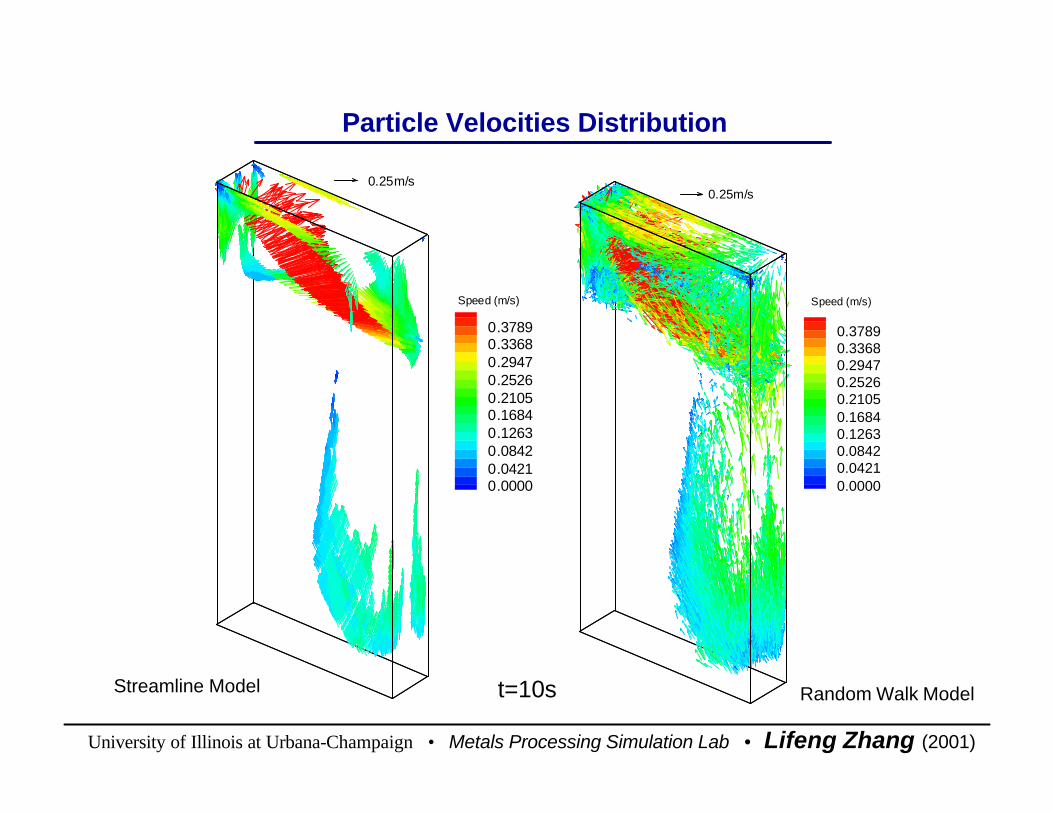
t=10s t=10s Streamline ModelStreamline Model Random Walk ModelRandom Walk Model
Particle Velocities DistributionParticle Velocities Distribution
0.37890.33680.29470.25260.21050.16840.12630.08420.04210.0000
0.25m/s
Speed (m/s)
0.37890.33680.29470.25260.21050.16840.12630.08420.04210.0000
0.25m/s
Speed (m/s)

University of Illinois at Urbana-Champaign • Metals Processing Simulation Lab • Lifeng Zhang (2001)
t=20s t=20s Streamline ModelStreamline Model Random Walk ModelRandom Walk Model
Particle Velocities DistributionParticle Velocities Distribution
0.37890.33680.29470.25260.21050.16840.12630.08420.04210.0000
0.25m/s
Speed (m/s)0.37890.33680.29470.25260.21050.16840.12630.08420.04210.0000
0.25m/s
Speed (m/s)
University of Illinois at Urbana-Champaign • Metals Processing Simulation Lab • Lifeng Zhang (2001)
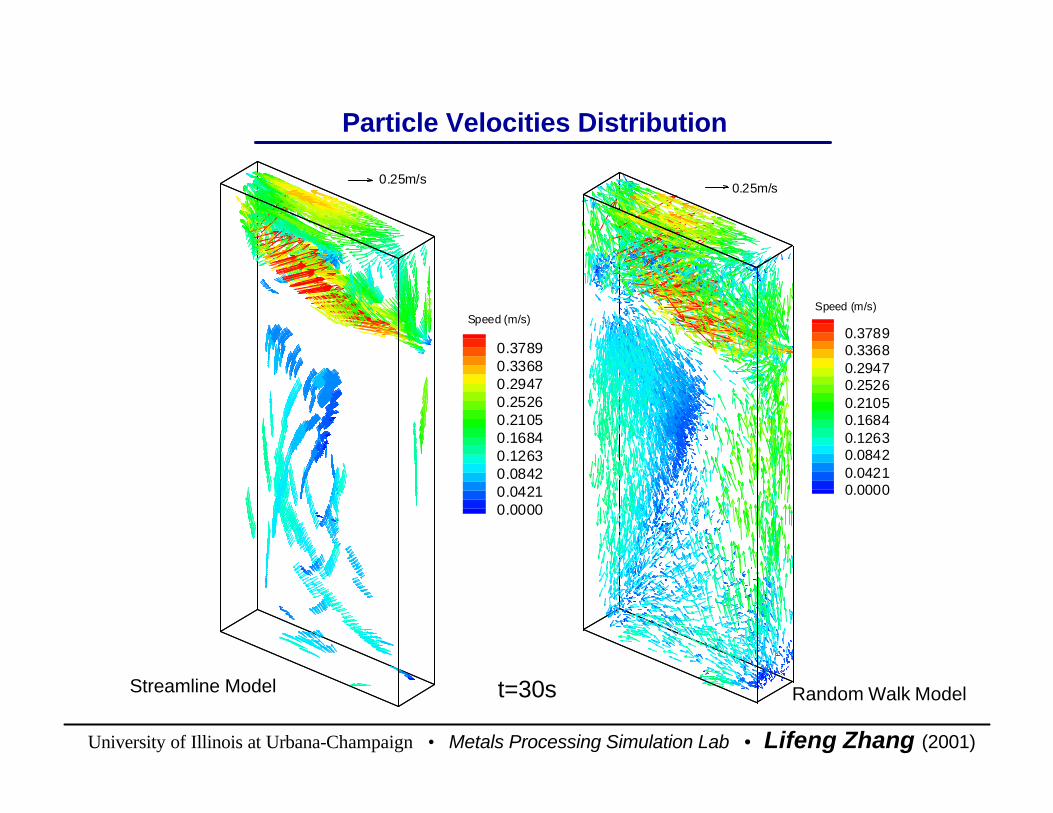
t=30s t=30s Streamline ModelStreamline Model Random Walk ModelRandom Walk Model
Particle Velocities DistributionParticle Velocities Distribution
0.37890.33680.29470.25260.21050.16840.12630.08420.04210.0000
0.25m/s
Speed (m/s)0.37890.33680.29470.25260.21050.16840.12630.08420.04210.0000
0.25m/s
Speed (m/s)

University of Illinois at Urbana-Champaign • Metals Processing Simulation Lab • Lifeng Zhang (2001)
t=100s t=100s Streamline ModelStreamline ModelRandom Walk ModelRandom Walk Model
Particle Velocities DistributionParticle Velocities Distribution
0.37890.33680.29470.25260.21050.16840.12630.08420.04210.0000
0.25m/s
Speed (m/s) 0.37890.33680.29470.25260.21050.16840.12630.08420.04210.0000
0.25m/s
Speed (m/s)

University of Illinois at Urbana-Champaign • Metals Processing Simulation Lab • Lifeng Zhang (2001)
Particle velocities (Streamline Model, 100s)Particle velocities (Streamline Model, 100s)
Particle velocities (Random Walk Model, 100s)Particle velocities (Random Walk Model, 100s)
Compare of Particle Velocities and Fluids Flow VelocitiesCompare of Particle Velocities and Fluids Flow Velocities
Fluid flow velocities (steady)Fluid flow velocities (steady)
0.37890.33680.29470.25260.21050.16840.12630.08420.04210.0000
0.25m/s
Speed (m/s)0.37890.33680.29470.25260.21050.16840.12630.08420.04210.0000
0.25m/s
Speed (m/s) 0.37890.33680.29470.25260.21050.16840.12630.08420.04210.0000
0.25m/s
Speed (m/s)
University of Illinois at Urbana-Champaign • Metals Processing Simulation Lab • Lifeng Zhang (2001)
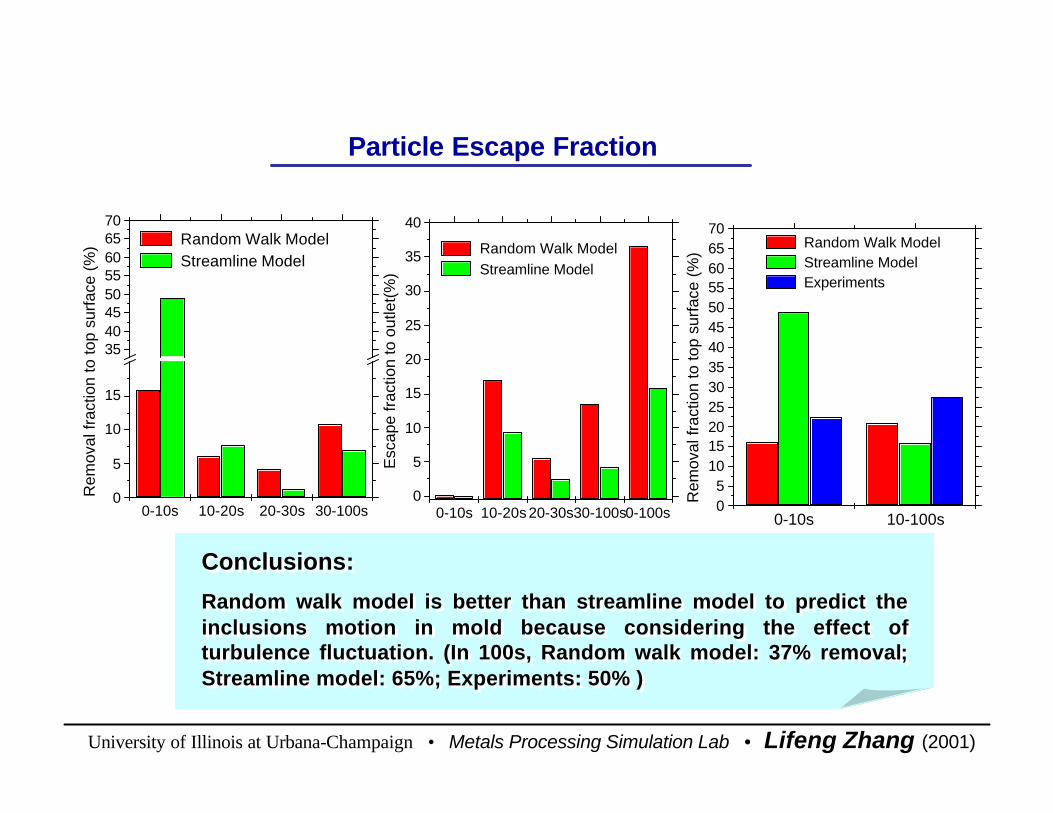
Particle Escape Fraction Particle Escape Fraction
0-10s 10-20s 20-30s 30-100s0
5
10
15
3540455055606570
Random Walk Model Streamline Model
Rem
oval
frac
tion
to to
p su
rfac
e (%
)
0-10s 10-100s05
10152025303540455055606570
Rem
oval
frac
tion
to to
p su
rfac
e (%
)
Random Walk Model Streamline Model Experiments
0-10s 10-20s 20-30s30-100s0-100s0
5
10
15
20
25
30
35
40
Random Walk Model Streamline Model
Esc
ape
frac
tion
to o
utle
t(%
)
Conclusions:
Random walk model is better than streamline model to predict theinclusions motion in mold because considering the effect of turbulence fluctuation. (In 100s, Random walk model: 37% removal; Streamline model: 65%; Experiments: 50% )
Conclusions:
Random walk model is better than streamline model to predict theinclusions motion in mold because considering the effect of turbulence fluctuation. (In 100s, Random walk model: 37% removal; Streamline model: 65%; Experiments: 50% )

University of Illinois at Urbana-Champaign • Metals Processing Simulation Lab • Lifeng Zhang (2001)
Comparison between Different Turbulence ModelsComparison between Different Turbulence Models
1. Large Eddy Simulation (LES)
2. Reynolds Stress Model (RSM)
3. k-ε Two Equation Model
1. Large Eddy Simulation (LES)
2. Reynolds Stress Model (RSM)
3. k-ε Two Equation Model
Non-uniform inlet conditionNon-uniform inlet condition
Uniform inlet conditionUniform inlet condition
1. k-ε Two Equation Model1. k-ε Two Equation Model
University of Illinois at Urbana-Champaign • Metals Processing Simulation Lab • Lifeng Zhang (2001)
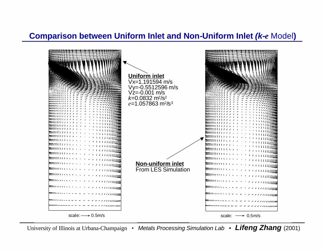
Comparison between Uniform Inlet and Non-Uniform Inlet (k-ε Model)Comparison between Uniform Inlet and Non-Uniform Inlet (k-ε Model)
scale: 0.5m/s scale: 0.5m/s
Uniform inletVx=1.191594 m/sVy=-0.5512596 m/sVz=-0.001 m/sk=0.0832 m2/s2
ε=1.057863 m2/s3
Uniform inletVx=1.191594 m/sVy=-0.5512596 m/sVz=-0.001 m/sk=0.0832 m2/s2
ε=1.057863 m2/s3
Non-uniform inletFrom LES SimulationNon-uniform inletFrom LES Simulation

University of Illinois at Urbana-Champaign • Metals Processing Simulation Lab • Lifeng Zhang (2001)
Comparison between Different Turbulence Models (Non-Uniform Inlet Condition)
Comparison between Different Turbulence Models (Non-Uniform Inlet Condition)
scale: 0.5m/s scale: 0.5m/s scale: 0.5m/s
K-εK-ε RSMRSM LESLES
University of Illinois at Urbana-Champaign • Metals Processing Simulation Lab • Lifeng Zhang (2001)
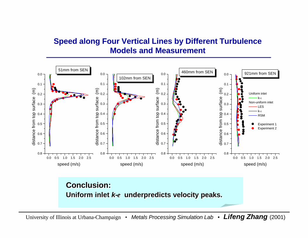
Speed along Four Vertical Lines by Different Turbulence Models and Measurement
Speed along Four Vertical Lines by Different Turbulence Models and Measurement
0.0 0.5 1.0 1.5 2.0 2.50.8
0.7
0.6
0.5
0.4
0.3
0.2
0.1
0.051mm from SEN
dist
ance
from
top
surf
ace
(m
)
speed (m/s)
0.0 0.5 1.0 1.5 2.0 2.50.8
0.7
0.6
0.5
0.4
0.3
0.2
0.1
0.0102mm from SEN
dist
ance
from
top
surf
ace
(m
)
speed (m/s)
0.0 0.5 1.0 1.5 2.0 2.50.8
0.7
0.6
0.5
0.4
0.3
0.2
0.1
0.0 460mm from SEN
dist
ance
from
top
surf
ace
(m
)
speed (m/s)
0.0 0.5 1.0 1.5 2.0 2.50.8
0.7
0.6
0.5
0.4
0.3
0.2
0.1
0.0
Uniform inlet k-ε
Non-uniform inlet LES k-ε RSM
Experiment 1 Experiment 2
921mm from SEN
dist
ance
from
top
surf
ace
(m
)
speed (m/s)
Conclusion: Uniform inlet k-ε underpredicts velocity peaks.Conclusion: Uniform inlet k-ε underpredicts velocity peaks.

University of Illinois at Urbana-Champaign • Metals Processing Simulation Lab • Lifeng Zhang (2001)
Enlargement of the Speed the line of 460mm from SEN on the central wide section
Enlargement of the Speed the line of 460mm from SEN on the central wide section
0.0 0.2 0.4 0.6 0.8 1.0 1.20.8
0.7
0.6
0.5
0.4
0.3
0.2
0.1
0.0
Uniform inlet k-ε
Non-uniform inlet LES k-ε RSM Experiment 1 Experiment 2
Peak of k-ε and LES
Peak of RSM and Experiments
460mm from SEN
dist
ance
from
top
surf
ace
(m
)
speed (m/s)
Conclusion:RSM model has slightly better prediction on the position of the peak for the line 460mm from SEN on the central wide section.
Conclusion:RSM model has slightly better prediction on the position of the peak for the line 460mm from SEN on the central wide section.
University of Illinois at Urbana-Champaign • Metals Processing Simulation Lab • Lifeng Zhang (2001)
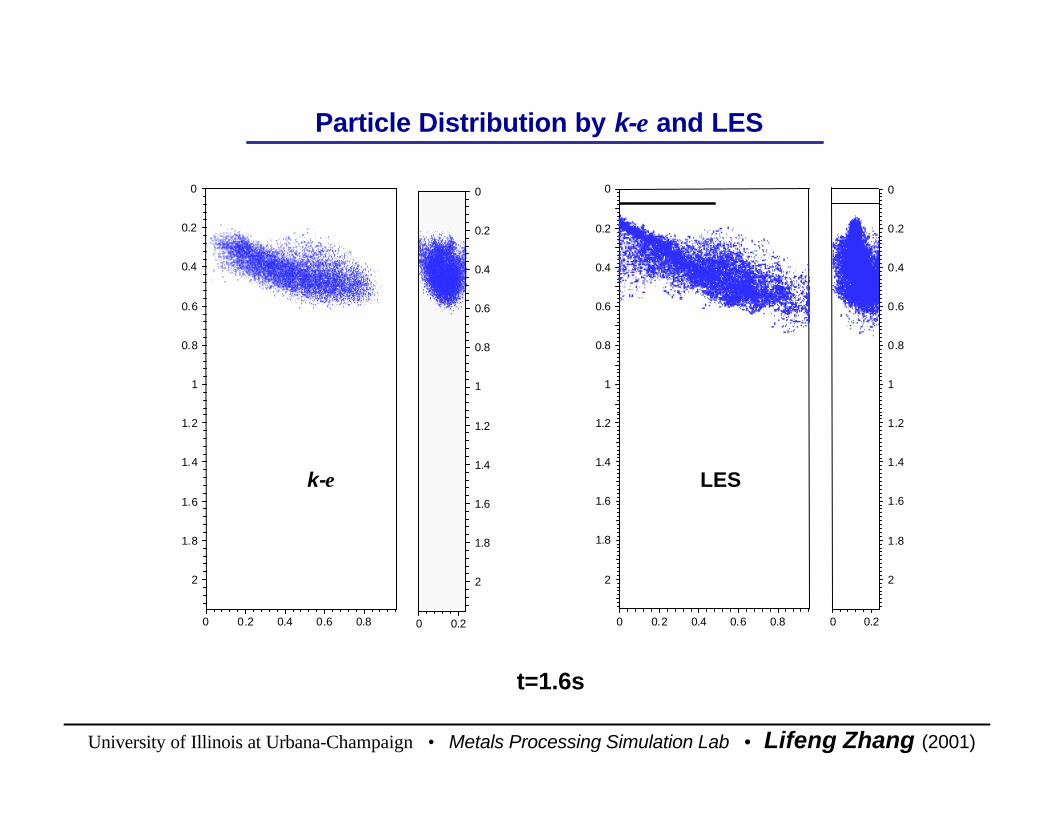
Particle Distribution by k-ε and LESParticle Distribution by k-ε and LES
0 0.2 0.4 0.6 0.8
0
0.2
0.4
0.6
0.8
1
1.2
1.4
1.6
1.8
2
0
0.2
0.4
0.6
0.8
1
1.2
1.4
1.6
1.8
2
0 0.20 0.2 0.4 0.6 0.8
0
0.2
0.4
0.6
0.8
1
1.2
1.4
1.6
1.8
2
0
0.2
0.4
0.6
0.8
1
1.2
1.4
1.6
1.8
2
0 0.2
k-εk-ε LESLES
t=1.6st=1.6s
University of Illinois at Urbana-Champaign • Metals Processing Simulation Lab • Lifeng Zhang (2001)
0 0.2 0.4 0.6 0.8
0
0.2
0.4
0.6
0.8
1
1.2
1.4
1.6
1.8
2
0 0.2
0
0.2
0.4
0.6
0.8
1
1.2
1.4
1.6
1.8
2
0
0.2
0.4
0.6
0.8
1
1.2
1.4
1.6
1.8
2
0 0.20 0.2 0.4 0.6 0.8
0
0.2
0.4
0.6
0.8
1
1.2
1.4
1.6
1.8
2
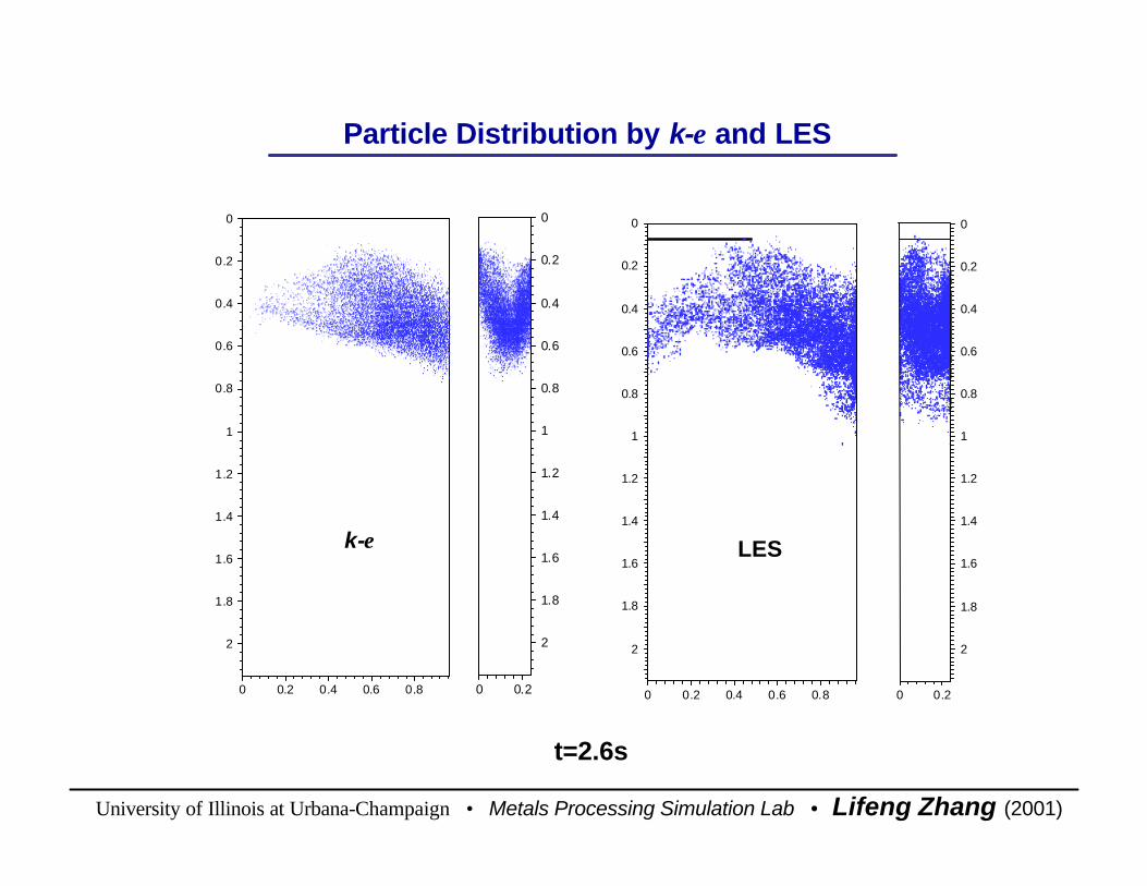
k-εk-ε LESLES
t=2.6st=2.6s
Particle Distribution by k-ε and LESParticle Distribution by k-ε and LES
University of Illinois at Urbana-Champaign • Metals Processing Simulation Lab • Lifeng Zhang (2001)
0
0.2
0.4
0.6
0.8
1
1.2
1.4
1.6
1.8
2
0 0.20 0.2 0.4 0.6 0.8
0
0.2
0.4
0.6
0.8
1
1.2
1.4
1.6
1.8
2
0 0.2 0.4 0.6 0.8
0
0.2
0.4
0.6
0.8
1
1.2
1.4
1.6
1.8
2
0 0.2
0
0.2
0.4
0.6
0.8
1
1.2
1.4
1.6
1.8
2
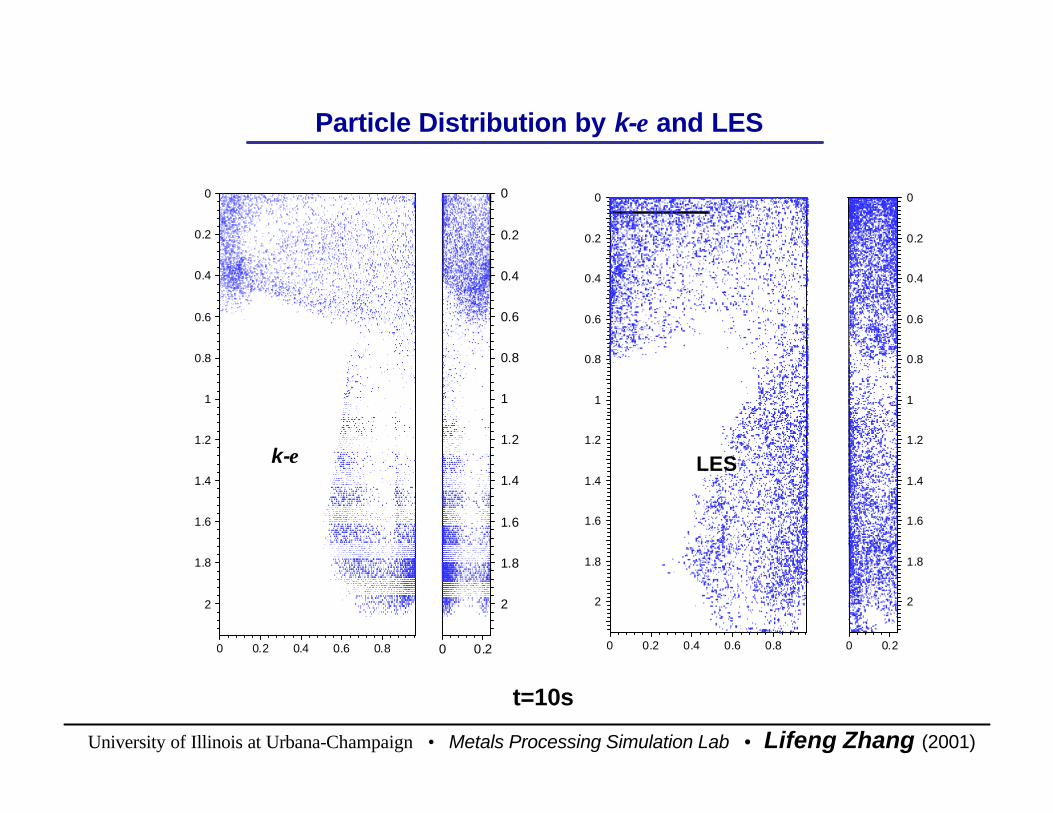
Particle Distribution by k-ε and LESParticle Distribution by k-ε and LES
k-εk-ε LESLES
t=10st=10s

University of Illinois at Urbana-Champaign • Metals Processing Simulation Lab • Lifeng Zhang (2001)
0
0.2
0.4
0.6
0.8
1
1.2
1.4
1.6
1.8
2
0 0.2
0
0.2
0.4
0.6
0.8
1
1.2
1.4
1.6
1.8
2
0 0.2 0.4 0.6 0.80 0.2
0
0.2
0.4
0.6
0.8
1
1.2
1.4
1.6
1.8
2
0 0.2 0.4 0.6 0.8
0
0.2
0.4
0.6
0.8
1
1.2
1.4
1.6
1.8
2
Particle Distribution by k-ε and LESParticle Distribution by k-ε and LES
k-εk-ε LESLES
t=100st=100s

University of Illinois at Urbana-Champaign • Metals Processing Simulation Lab • Lifeng Zhang (2001)
Particle Escape Fraction Particle Escape Fraction
Conclusion:Ù RSM model has a best prediction of particle removal
fraction compared to the experiments results. Ù LES model overpredicts particle removal fraction
and k-ε far underpredicts particle removal fraction.
Conclusion:Ù RSM model has a best prediction of particle removal
fraction compared to the experiments results. Ù LES model overpredicts particle removal fraction
and k-ε far underpredicts particle removal fraction.
0-10s 10-100s 0-100s0
10
20
30
40
19%
13%
37%
Fra
ctio
n to
out
let (
%)
k-ε LES RSM
0-10s 10-100s 0-100s1015202530354045505560657075
50%
57%
66%
36%
R
emov
al fr
actio
n to
top
surf
ace
(%)
k-ε LES RSM Experiment
University of Illinois at Urbana-Champaign • Metals Processing Simulation Lab • Lifeng Zhang (2001)
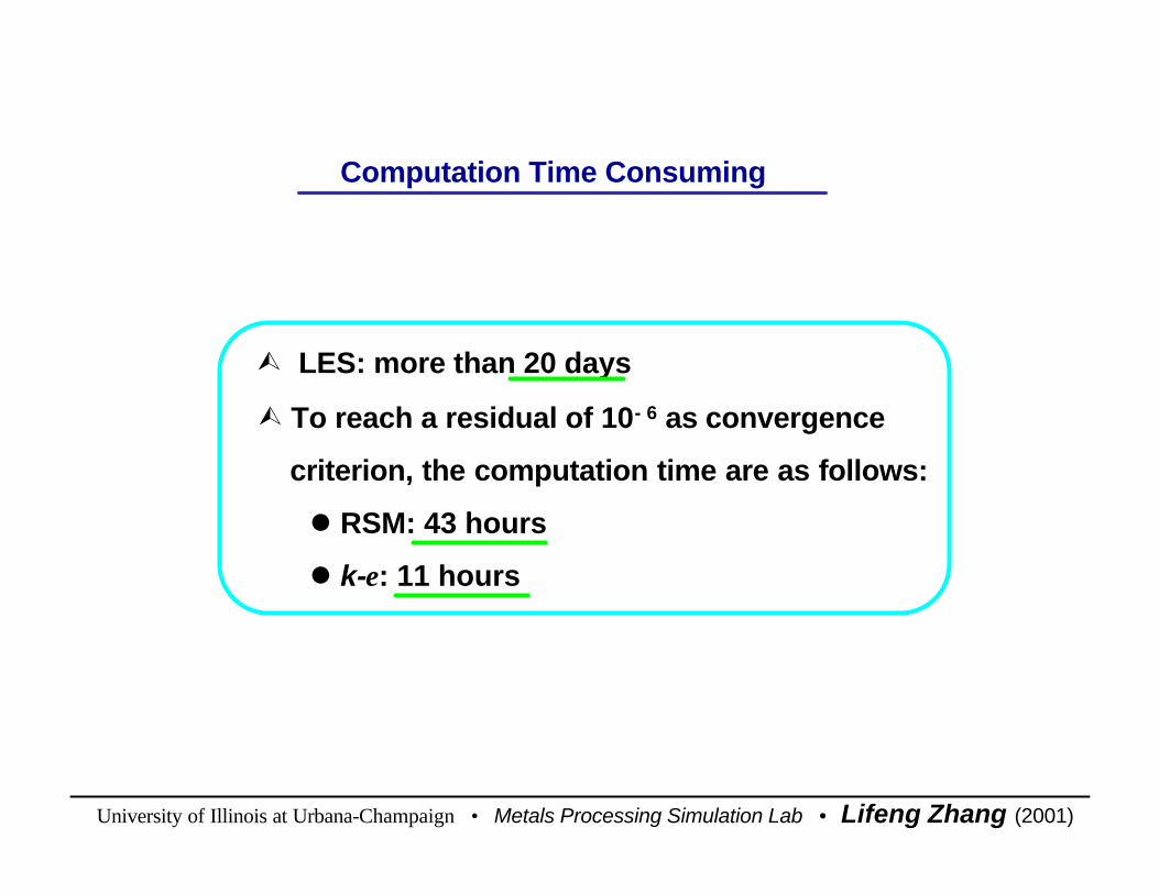
Computation Time Consuming Computation Time Consuming
Ù To reach a residual of 10- 6 as convergence
criterion, the computation time are as follows:
l RSM: 43 hours
l k-ε: 11 hours
Ù To reach a residual of 10- 6 as convergence
criterion, the computation time are as follows:
l RSM: 43 hours
l k-ε: 11 hours
Ù LES: more than 20 daysÙ LES: more than 20 days

University of Illinois at Urbana-Champaign • Metals Processing Simulation Lab • Lifeng Zhang (2001)
Fluid Flow and Inclusion Behavior in Steel Caster
(Random Walk k-ε)
Fluid Flow and Inclusion Behavior in Steel Caster
(Random Walk k-ε)
University of Illinois at Urbana-Champaign • Metals Processing Simulation Lab • Lifeng Zhang (2001)
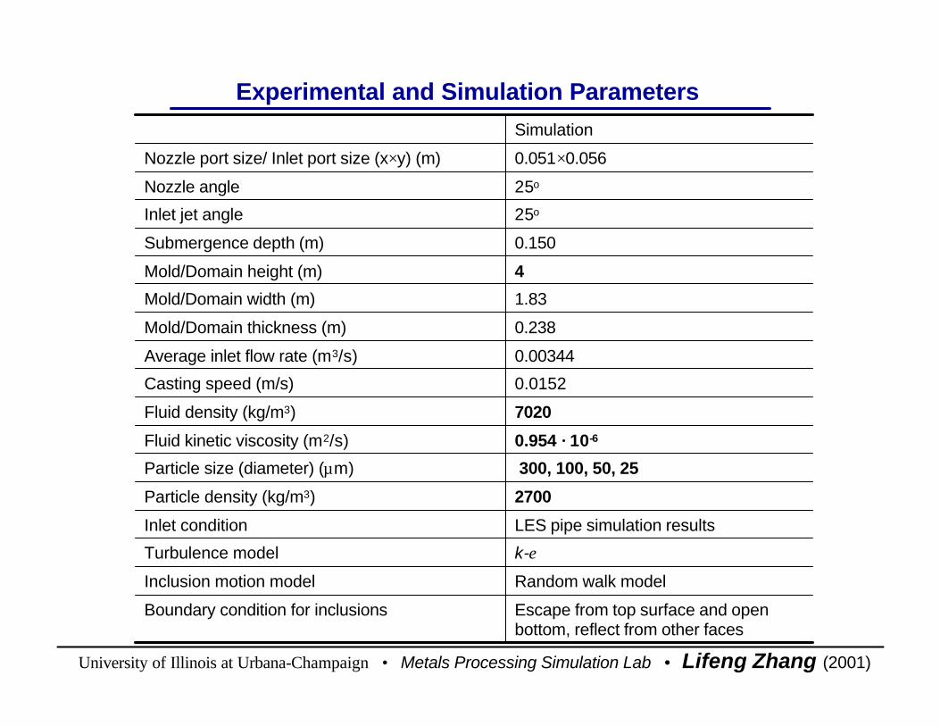
Escape from top surface and open bottom, reflect from other faces
Boundary condition for inclusions
Random walk modelInclusion motion model
k-εTurbulence model
LES pipe simulation resultsInlet condition
2700Particle density (kg/m3)
300, 100, 50, 25Particle size (diameter) (µm)
0.954 ×10⁻⁶Fluid kinetic viscosity (m2/s)
7020Fluid density (kg/m3)
0.0152Casting speed (m/s)
0.00344Average inlet flow rate (m3/s)
0.238Mold/Domain thickness (m)
1.83Mold/Domain width (m)
4Mold/Domain height (m)
0.150Submergence depth (m)
25oInlet jet angle
25oNozzle angle
0.051×0.056Nozzle port size/ Inlet port size (x×y) (m)
Simulation
Experimental and Simulation ParametersExperimental and Simulation Parameters

University of Illinois at Urbana-Champaign • Metals Processing Simulation Lab • Lifeng Zhang (2001)
00.511.522.533.5
distance from top surface (m)
0
0.2
0.4
0.6
0.8
distancefron
nozzlecenter(m
)
00.511.522.533.5
distance from top surface (m)
0
0.2
0.4
0.6
0.8
distancefron
nozzlecenter(m
)
1m/s
Mesh and Velocity Distribution at Central FaceMesh and Velocity Distribution at Central Face

University of Illinois at Urbana-Champaign • Metals Processing Simulation Lab • Lifeng Zhang (2001)
0
0 .2
0 .4
0 .6
0 .8
1 m /s
Magnified Velocity Distribution on Central faceMagnified Velocity Distribution on Central face

University of Illinois at Urbana-Champaign • Metals Processing Simulation Lab • Lifeng Zhang (2001)
0 0.2 0.4 0.6 0.8
distance from nozzle center (m)
0
0.5
1
1.5
2
2.5
3
3.5
diatancefrom
topsurface
(m)
0 0.2 0.4 0.6 0.8
distance from nozzle center (m)
0
0.5
1
1.5
2
2.5
3
3.5
diatancefrom
topsurface
(m)
0 0.2 0.4 0.6 0.8
distance from nozzle center (m)
0
0.5
1
1.5
2
2.5
3
3.5
diatancefrom
topsurface
(m)
0 0.2 0.4 0.6 0.8
distance from nozzle center (m)
0
0.5
1
1.5
2
2.5
3
3.5
diatancefrom
topsurface
(m)
300µm300µm 50µm50µm 300µm300µm 50µm50µm
1.6s1.6s 40s40s
Different Size Particle distribution Different Size Particle distribution

University of Illinois at Urbana-Champaign • Metals Processing Simulation Lab • Lifeng Zhang (2001)
0-10s 10-20s 20-30s 30-40s0
5
10
15
20
25
30
300µm 100µm 50µm 25µm
rem
oval
frac
tion
to to
p su
rfac
e (%
)
time period
Escape Fraction for Different Size Inclusions Escape Fraction for Different Size Inclusions
Conclusions:l With increasing size, inclusion removal to the top surface becomes easier. l Smaller inclusions are much easily transported by the flow out of the bottom.
Conclusions:l With increasing size, inclusion removal to the top surface becomes easier. l Smaller inclusions are much easily transported by the flow out of the bottom.
top surface open bottom
10
20
30
40
50
60100s
11.6%
30%33%34%
33%
27%25%
60%
Fra
ctio
n (%
)
25µm 50µm 100µm 300µm
10010
100
100s
20 400
rem
oval
frac
tion
(%
)
inclusion size (µm)

University of Illinois at Urbana-Champaign • Metals Processing Simulation Lab • Lifeng Zhang (2001)
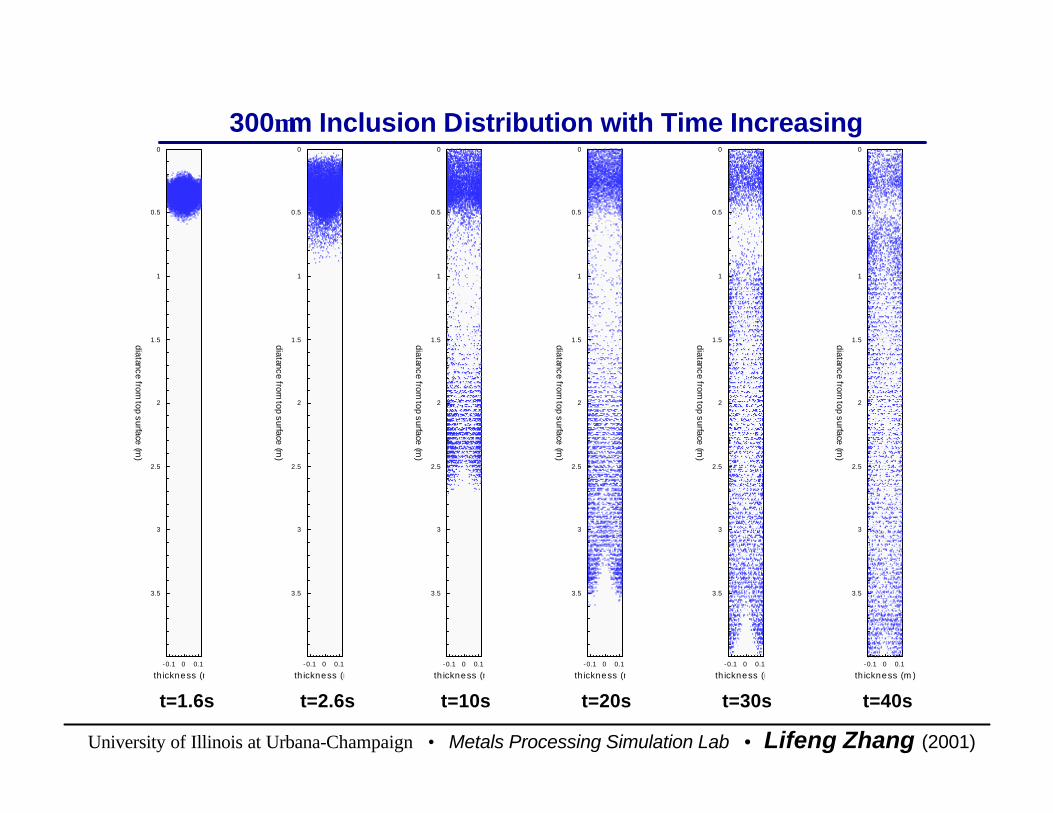
300µm Inclusion Distribution with Time Increasing300µm Inclusion Distribution with Time Increasing
0 0.2 0.4 0.6 0.8
distance from nozzle center (m)
0
0.5
1
1.5
2
2.5
3
3.5
diatancefro
mtop
surface(m
)
0 0.2 0.4 0.6 0.8
distance from nozzle center (m)
0
0.5
1
1.5
2
2.5
3
3.5
diatancefro
mtop
surface(m
)
0 0.2 0.4 0.6 0.8
distance from nozzle center (m)
0
0.5
1
1.5
2
2.5
3
3.5
diatancefro
mtop
surface(m
)
0 0.2 0.4 0.6 0.8
distance from nozzle center (m)
0
0.5
1
1.5
2
2.5
3
3.5
diatancefro
mtop
surface(m
)
t=1.6st=1.6s t=2.6st=2.6s t=10st=10s t=20st=20s

University of Illinois at Urbana-Champaign • Metals Processing Simulation Lab • Lifeng Zhang (2001)
0 0.2 0.4 0.6 0.8
distance from nozzle center (m)
0
0.5
1
1.5
2
2.5
3
3.5
diata
ncefrom
topsu
rface(m
)
0 0.2 0.4 0.6 0.8
distance from nozzle center (m)
0
0.5
1
1.5
2
2.5
3
3.5
diata
ncefrom
topsu
rface(m
)
0 0.2 0.4 0.6 0.8
distance from nozzle center (m)
0
0.5
1
1.5
2
2.5
3
3.5
diata
ncefrom
topsu
rface(m
)
0 0.2 0.4 0.6 0.8
distance from nozzle center (m)
0
0.5
1
1.5
2
2.5
3
3.5
diata
ncefrom
topsu
rface(m
)
t=30st=30s t=40st=40s t=100st=100s t=168.7st=168.7s
300µm Inclusion Distribution with Time Increasing300µm Inclusion Distribution with Time Increasing

University of Illinois at Urbana-Champaign • Metals Processing Simulation Lab • Lifeng Zhang (2001)
0 0.2 0.4 0.6 0.8
distance from nozzle center (m)
0
0.5
1
1.5
2
2.5
3
3.5
diatancefrom
topsurface
(m)
0 0.2 0.4 0.6 0.8
distance from nozzle center (m)
0
0.5
1
1.5
2
2.5
3
3.5
diatancefrom
topsurface
(m)
0 0.2 0.4 0.6 0.8
distance from nozzle center (m)
0
0.5
1
1.5
2
2.5
3
3.5
diatancefrom
topsurface
(m)
0 0.2 0.4 0.6 0.8
distance from nozzle center (m)
0
0.5
1
1.5
2
2.5
3
3.5
diatancefrom
topsurface
(m)
0 0.2 0.4 0.6 0.8
distance from nozzle center (m)
0
0.5
1
1.5
2
2.5
3
3.5
diatancefrom
topsurface
(m)
t=200st=200s t=400st=400st=348.7st=348.7st=298.7st=298.7st=248.7t=248.7
300µm Inclusion Distribution with Time Increasing300µm Inclusion Distribution with Time Increasing

University of Illinois at Urbana-Champaign • Metals Processing Simulation Lab • Lifeng Zhang (2001)
Conclusion from simulation:
Inclusion amount at the center of mold is less than that at other places.
Conclusion from simulation:
Inclusion amount at the center of mold is less than that at other places.
Microscope observation S print0
1
2
3
4
5
1/4 slab wideness 1/2 slab wideness
incl
usio
n am
ount
(1/c
m2 )
Conclusion about Inclusion Distribution along Slab WidenessConclusion about Inclusion Distribution along Slab Wideness
Proof from industrial experimentsProof from industrial experiments
ìììì
University of Illinois at Urbana-Champaign • Metals Processing Simulation Lab • Lifeng Zhang (2001)
-0.1 0 0.1
th ickness (m )
0
0.5
1
1.5
2
2.5
3
3.5
diatancefrom
topsurface
(m)
-0.1 0 0.1
th ickness (m )
0
0.5
1
1.5
2
2.5
3
3.5
diatancefrom
topsurface
(m)
-0.1 0 0.1
th ickness (m )
0
0.5
1
1.5
2
2.5
3
3.5
diatancefrom
topsurface
(m)
-0.1 0 0.1
th ickness (m )
0
0.5
1
1.5
2
2.5
3
3.5
diatancefrom
topsurface
(m)
-0.1 0 0.1
th ickness (m )
0
0.5
1
1.5
2
2.5
3
3.5
diatancefrom
topsurface
(m)
-0.1 0 0.1
th ickness (m )
0
0.5
1
1.5
2
2.5
3
3.5
diatancefrom
topsurface
(m)
t=1.6s t=2.6s t=10s t=20s t=30s t=40st=1.6s t=2.6s t=10s t=20s t=30s t=40s
300µm Inclusion Distribution with Time Increasing300µm Inclusion Distribution with Time Increasing

University of Illinois at Urbana-Champaign • Metals Processing Simulation Lab • Lifeng Zhang (2001)
-0.1 0 0.1
th ickness (m )
0
0 .5
1
1 .5
2
2 .5
3
3 .5
diatancefrom
topsurface
(m)
-0.1 0 0.1
th ickness (m )
0
0 .5
1
1 .5
2
2 .5
3
3 .5
diatancefrom
topsurface
(m)
-0.1 0 0.1
th ickness (m )
0
0 .5
1
1 .5
2
2 .5
3
3 .5
diatancefrom
topsurface
(m)
-0. 1 0 0 .1
th ic kness (m)
0
0.5
1
1.5
2
2.5
3
3.5
diatancefrom
topsurface
(m)
-0.1 0 0.1
th ickness (m )
0
0 .5
1
1 .5
2
2 .5
3
3 .5
diatancefrom
topsurface
(m)
-0.1 0 0.1
th ickness (m )
0
0 .5
1
1 .5
2
2 .5
3
3 .5
diatancefrom
topsurface
(m)
t=100s t=168.7s t=200s t=248.7s t=298.7s t=400st=100s t=168.7s t=200s t=248.7s t=298.7s t=400s
300µm Inclusion Distribution with Time Increasing300µm Inclusion Distribution with Time Increasing

University of Illinois at Urbana-Champaign • Metals Processing Simulation Lab • Lifeng Zhang (2001)
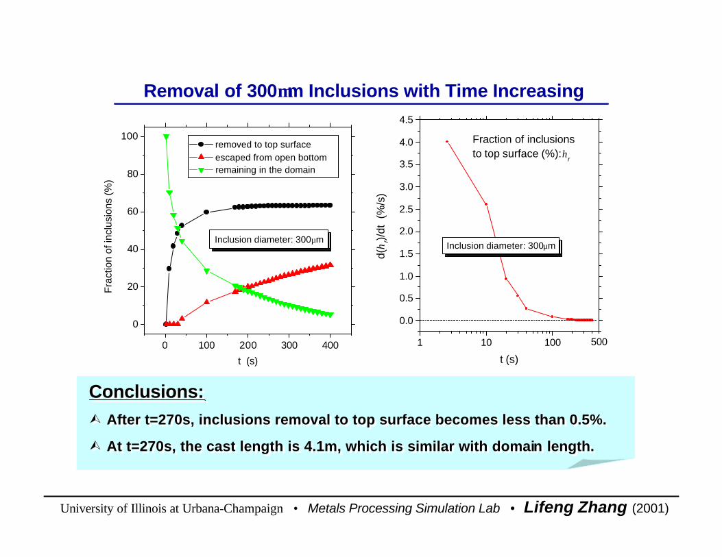
Removal of 300µm Inclusions with Time IncreasingRemoval of 300µm Inclusions with Time Increasing
ConclusionsÙ Inclusions require about 10min to leave the domain of mold region (4m). Ù The total removal fraction to top surface is 63%, escape fraction to open bottom is 37%.Ù In 10 min, the casting length is 8.24m, but the domain is 4m. So if ignoring the inclusions entrapment to solidified shell, the steel in the domain will become dirty more and more with time increasing
ConclusionsÙ Inclusions require about 10min to leave the domain of mold region (4m). Ù The total removal fraction to top surface is 63%, escape fraction to open bottom is 37%.Ù In 10 min, the casting length is 8.24m, but the domain is 4m. So if ignoring the inclusions entrapment to solidified shell, the steel in the domain will become dirty more and more with time increasing
200 250 300 350 4000
2
4
6
8
10
12
14
16
18
20
Calculation Fitting of calculation
η remain= - 5.17+22.8 exp[((200-t)/252)]
frac
tion
of in
clus
ions
rem
aini
ng in
dom
ain,
ηre
mai
n (%
)
time (s)
0 100 200 300 400 500 600
0
20
40
60
80
100
t=542s
Calculation Extroplation
Fra
ctio
n of
incl
usio
ns r
emai
ning
in d
omai
n (%
)
t (s)
University of Illinois at Urbana-Champaign • Metals Processing Simulation Lab • Lifeng Zhang (2001)
Conclusions:Ù After t=270s, inclusions removal to top surface becomes less than 0.5%.
Ù At t=270s, the cast length is 4.1m, which is similar with domain length.
Conclusions:Ù After t=270s, inclusions removal to top surface becomes less than 0.5%.
Ù At t=270s, the cast length is 4.1m, which is similar with domain length.
Removal of 300µm Inclusions with Time IncreasingRemoval of 300µm Inclusions with Time Increasing
1 10 100
0.0
0.5
1.0
1.5
2.0
2.5
3.0
3.5
4.0
4.5
500
Inclusion diameter: 300µm
Fraction of inclusions to top surface (%):η
r
t (s)
d(η
r)/dt
(%
/s)
0 100 200 300 400
0
20
40
60
80
100
Inclusion diameter: 300µm
removed to top surface escaped from open bottom remaining in the domain
Fra
ctio
n of
incl
usio
ns (%
)
t (s)

University of Illinois at Urbana-Champaign • Metals Processing Simulation Lab • Lifeng Zhang (2001)
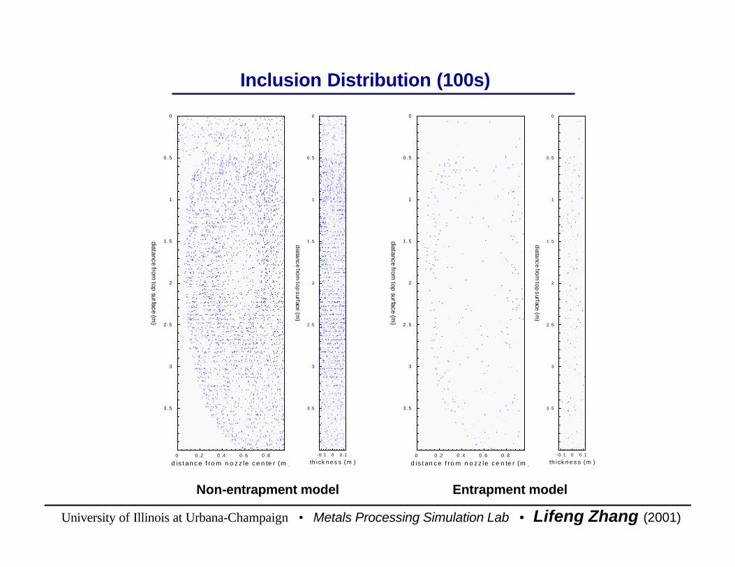
Effect of Inclusion Entrapment to Solidified ShellEffect of Inclusion Entrapment to Solidified Shell
l Non-Entrapment Model: previous simulations assume that if inclusions collide with solidified shell, they will be reflected.
l Entrapment Model: if inclusions collide with solidified shell, they will be entrapped.
l Non-Entrapment Model: previous simulations assume that if inclusions collide with solidified shell, they will be reflected.
l Entrapment Model: if inclusions collide with solidified shell, they will be entrapped.

University of Illinois at Urbana-Champaign • Metals Processing Simulation Lab • Lifeng Zhang (2001)
0-10s 10-100s0
5
10
15
20
25
30
35
40Entrapment Model
Top surface Narrow face Wide faces Bottom
0% 1%
Incl
usio
n fr
actio
n to
face
s (%
)
0-10s 10-100s0
5
10
15
20
25
30
35
40Non-Entrapment Model
Top surface Bottom
0%
Incl
usio
n fr
actio
n to
face
s (%
)
Entrapment Model: Top surface: 23%, entrapped to wide faces: 54%, narrow face: 19%, flow away from bottom: 1%, remain in domain: 3% (Total escape in 100s: 97%)
Non-Entrapment model: Top surface: 60%, flow away from bottom: 12%, remain in domain: 28% (Total escape in 100s: 72%)
Entrapment Model: Top surface: 23%, entrapped to wide faces: 54%, narrow face: 19%, flow away from bottom: 1%, remain in domain: 3% (Total escape in 100s: 97%)
Non-Entrapment model: Top surface: 60%, flow away from bottom: 12%, remain in domain: 28% (Total escape in 100s: 72%)
Effect of Inclusion Entrapment to Solidified Shell (100s)Effect of Inclusion Entrapment to Solidified Shell (100s)

University of Illinois at Urbana-Champaign • Metals Processing Simulation Lab • Lifeng Zhang (2001)
0 0 . 2 0. 4 0 .6 0 .8
d is ta nce f rom no zz le ce nte r (m )
0
0. 5
1
1. 5
2
2. 5
3
3. 5
diatancefro
mtop
surface(m
)
-0 .1 0 0 .1
th ic kness (m )
0
0 .5
1
1 .5
2
2 .5
3
3 .5
diatancefrom
topsurface
(m)
0 0 .2 0 .4 0 .6 0 .8
dis tan ce fro m n ozz le cent er (m)
0
0 . 5
1
1 . 5
2
2 . 5
3
3 . 5
diatancefro
mtop
surface(m
)
-0.1 0 0 .1
th ick nes s (m )
0
0 .5
1
1 .5
2
2 .5
3
3 .5
diatancefrom
topsurface
(m)
Inclusion Distribution (10s)Inclusion Distribution (10s)
Non-entrapment modelNon-entrapment model Entrapment modelEntrapment model
University of Illinois at Urbana-Champaign • Metals Processing Simulation Lab • Lifeng Zhang (2001)
0 0 .2 0 .4 0 .6 0 . 8
d is t an c e f ro m n o z z le c e n te r (m )
0
0 . 5
1
1 . 5
2
2 . 5
3
3 . 5
diatancefrom
topsurface
(m)
- 0. 1 0 0 .1
th i ck n e s s ( m )
0
0 .5
1
1 .5
2
2 .5
3
3 .5
diatancefrom
topsurface
(m)
0 0 .2 0 .4 0 .6 0 . 8
d is t an c e f ro m n o z z le c e n te r (m )
0
0 . 5
1
1 . 5
2
2 . 5
3
3 . 5
diatancefrom
topsurface
(m)
- 0. 1 0 0 .1
th i ck n e s s ( m )
0
0 .5
1
1 .5
2
2 .5
3
3 .5
diatancefrom
topsurface
(m)
Non-entrapment modelNon-entrapment model Entrapment modelEntrapment model
Inclusion Distribution (100s)Inclusion Distribution (100s)
University of Illinois at Urbana-Champaign • Metals Processing Simulation Lab • Lifeng Zhang (2001)
The Accuracy of the Similarity Criterion of Stokes Velocity for the Particle Motion in Water and in Liquid Steel
The Accuracy of the Similarity Criterion of Stokes Velocity for the Particle Motion in Water and in Liquid Steel

University of Illinois at Urbana-Champaign • Metals Processing Simulation Lab • Lifeng Zhang (2001)
The Accuracy of the Similarity of the Particle Motion between Water and Liquid Steel Stokes Velocity
The Accuracy of the Similarity of the Particle Motion between Water and Liquid Steel Stokes Velocity
Two holes on lower part of one wide faceOutlet
9882700Particle density (kg/m3)
3.8mm473 µmParticle size
1.0×10 - 60.954×10⁻⁶Viscosity (m2/s)
9987020Density (kg/m3)
Same (The previous water model case)Mold Geometry
Water Model Steel Caster
( ) gdV PPs µ
ρρ18
2−=The Stokes velocity of the particles in water is the same as that of the inclusions in liquid steel. (Vs=0.0786m/s)
The Stokes velocity of the particles in water is the same as that of the inclusions in liquid steel. (Vs=0.0786m/s)

University of Illinois at Urbana-Champaign • Metals Processing Simulation Lab • Lifeng Zhang (2001)
( ) gdV PPs µ
ρρ18
2−=
VS: Stokes velocity, m/s
ρ, ρp, liquid and particle density, kg/m3
dp, particle diameter, m
µ, liquid viscosity, kg/m.s
g, gravitational acceleration, m/s2
Ap: Intersection area of particle, m2
VS: Stokes velocity, m/s
ρ, ρp, liquid and particle density, kg/m3
dp, particle diameter, m
µ, liquid viscosity, kg/m.s
g, gravitational acceleration, m/s2
Ap: Intersection area of particle, m2
Particle Stokes Terminal Rising Velocity in Liquid Particle Stokes Terminal Rising Velocity in Liquid
( ) 32
61
21
PPPPD dgAuC πρρρ −=
Force balance on particle: Drag force=gravitational forceForce balance on particle: Drag force=gravitational force
PDC
Re24
=
1Re <pForFor

University of Illinois at Urbana-Champaign • Metals Processing Simulation Lab • Lifeng Zhang (2001)
( )g
dV PP
s µρρ
18
2−=
VS: Stokes velocity, m/s
ρ, ρp, liquid and particle density, kg/m3
dp, particle diameter, m
µ, liquid viscosity, kg/m.s
g, gravitational acceleration, m/s2
VS: Stokes velocity, m/s
ρ, ρp, liquid and particle density, kg/m3
dp, particle diameter, m
µ, liquid viscosity, kg/m.s
g, gravitational acceleration, m/s2
Particle Stokes Terminal Rising Velocity in Liquid Particle Stokes Terminal Rising Velocity in Liquid
10-6 10-5 10-4 10-3 10-210
-7
10-6
10-5
10-4
10-3
10-2
10-1
100
Liquid steel system:
ρp=2700kg/m3
ρ=7020kg/m3 µ=0.0067kg/m.s
Water model system:
ρp=988kg/m3
ρ=998kg/m3 µ=0.001kg/m.s
Sto
kes
velo
sity
of p
artic
les
(m/s
)
dp (m)

University of Illinois at Urbana-Champaign • Metals Processing Simulation Lab • Lifeng Zhang (2001)
Comparison Between Liquid Steel and Water Model Comparison Between Liquid Steel and Water Model
0-10s 10-20s 20-30s0
5
10
15
20
25
30
35
40
45
50
55
Particles in water and liquid steelhave the same Stokes Velocity
dp=473µm, ρp=2700 kg/m3
in liquid steel
dp=3.8mm, ρp=988 kg/m3
in water
rem
oval
frac
tion
to to
p su
rfac
e (%
)
time period
The difference of particle removal fraction in water and liquid steel shows that the Stokes rising velocity is not a reasonable criterion for matching the particle behavior in water with inclusion behavior in liquid steel.
The difference of particle removal fraction in water and liquid steel shows that the Stokes rising velocity is not a reasonable criterion for matching the particle behavior in water with inclusion behavior in liquid steel.
top surface outlet 0
10
20
30
40
50
60
70
80
have the same Stokes VelocityParticles in water and liquid steel
100s
dp=473µm, ρ
p=2700 kg/m3
in liquid steel
dp=3.8mm, ρp=988 kg/m3
in water
Esc
ape
frac
tion
in 1
00s
(%)

University of Illinois at Urbana-Champaign • Metals Processing Simulation Lab • Lifeng Zhang (2001)
Comparison Between Liquid Steel and Water Model Comparison Between Liquid Steel and Water Model
0-10s 10-20s 20-30s0
5
10
15
20
25
30
dp=300µm, ρ
p=2700 kg/m3
in liquid steel
dp=3.8mm, ρp=988 kg/m3
in water
rem
oval
frac
tion
to to
p su
rfac
e (%
)
time periodtop surface outlet
0
10
20
30
40
50
60
100s
dp=300µm, ρp=2700 kg/m3
in liquid steel
dp=3.8mm, ρp=988 kg/m3
in water
Esc
ape
frac
tion
in 1
00s
(%)
Steel caster: Previous Steel caster case (length : 4m, open bottom as outlet)
Water Model: Previous Water Model (length:2.152m, two holes at under part of wide face as outlet)
Steel caster: Previous Steel caster case (length : 4m, open bottom as outlet)
Water Model: Previous Water Model (length:2.152m, two holes at under part of wide face as outlet)
Stokes Velocity: Inclusions in steel 0.0316m/s
Particles in water 0.0786m/s
Stokes Velocity: Inclusions in steel 0.0316m/s
Particles in water 0.0786m/s
University of Illinois at Urbana-Champaign • Metals Processing Simulation Lab • Lifeng Zhang (2001)
Pressure on the Top Surface and Level Fluctuation of MoldPressure on the Top Surface and Level Fluctuation of Mold
University of Illinois at Urbana-Champaign • Metals Processing Simulation Lab • Lifeng Zhang (2001)
918Top oil density
0.0295Nozzle outer diameter (m)
0.0195Nozzle inner diameter (m)
Uniform inlet velocity and k, εInlet condition (Nozzle)
1.0 ×10⁻⁶Fluid kinetic viscosity (m2/s)
1000Fluid density (kg/m3)
0.0173Casting speed (m/s)
4.67 ×10⁻⁴Average inlet flow rate (m3/s)
0.059Mold/Domain thickness (m)
0.457Mold/Domain width (m)
0.686Mold/Domain height (m)
0.150Submergence depth (m)
25o downwardInlet jet angle
20o downwardNozzle angle
0.0175×0.0175Nozzle port size/ Inlet port size (x×y) (m)
Experiment
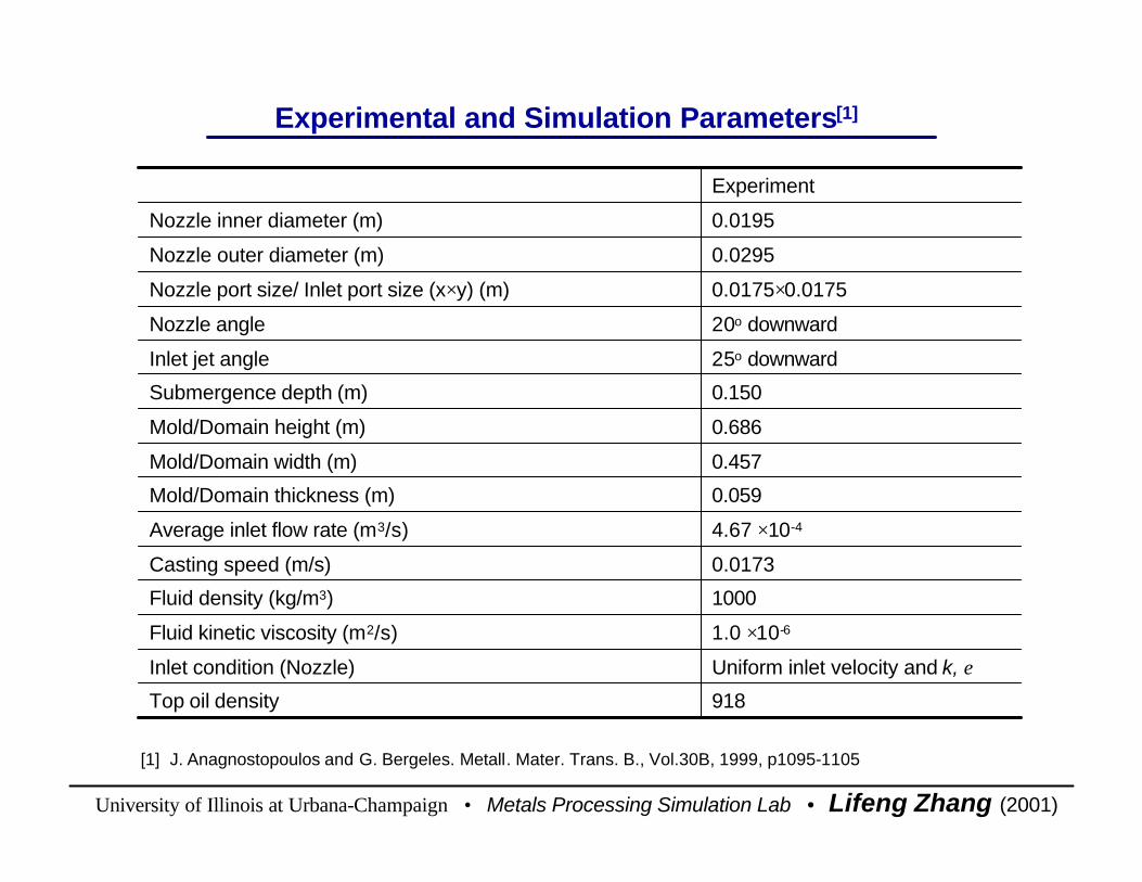
Experimental and Simulation Parameters[1]Experimental and Simulation Parameters[1]
[1] J. Anagnostopoulos and G. Bergeles. Metall. Mater. Trans. B., Vol.30B, 1999, p1095-1105[1] J. Anagnostopoulos and G. Bergeles. Metall. Mater. Trans. B., Vol.30B, 1999, p1095-1105

University of Illinois at Urbana-Champaign • Metals Processing Simulation Lab • Lifeng Zhang (2001)
Mesh and Velocity Distribution Mesh and Velocity Distribution
0 0.1 0.2
-0.6
-0.5
-0.4
-0.3
-0.2
-0.1
X
Y
Z
0 0.1 0.2
-0.6
-0.5
-0.4
-0.3
-0.2
-0.1
X
Y
Z
1m/s
0 0.01-0.18
-0.16
-0.14
-0.12
-0.1
-0.08
-0.06
-0.04
-0.02
0
0 0.02-0.18
-0.16
-0.14
-0.12
-0.1
-0.08
-0.06
-0.04
-0.02
0
1m/s
NozzleNozzle MoldMold
University of Illinois at Urbana-Champaign • Metals Processing Simulation Lab • Lifeng Zhang (2001)
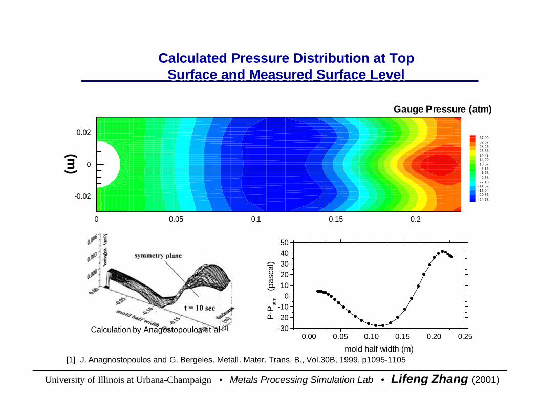
0.00 0.05 0.10 0.15 0.20 0.25-30-20-10
01020304050
P-P
atm
(pas
cal)
mold half width (m)
-0.02
0
0.02
(m)
0 0.05 0.1 0.15 0.2
37.0932.6728.2523.8319.4114.9910.57
6.151.73
-2.68-7.10
-11.52-15.94-20.36-24.78
Gauge Pressure (atm)
Calculation by Anagostopoulos et al [1]Calculation by Anagostopoulos et al [1]
[1] J. Anagnostopoulos and G. Bergeles. Metall. Mater. Trans. B., Vol.30B, 1999, p1095-1105[1] J. Anagnostopoulos and G. Bergeles. Metall. Mater. Trans. B., Vol.30B, 1999, p1095-1105
Calculated Pressure Distribution at Top Surface and Measured Surface Level
Calculated Pressure Distribution at Top Surface and Measured Surface Level

University of Illinois at Urbana-Champaign • Metals Processing Simulation Lab • Lifeng Zhang (2001)
Mold Surface Level Calculated from Pressure at Center Line along Width direction on Top Surface
Mold Surface Level Calculated from Pressure at Center Line along Width direction on Top Surface
0.00 0.05 0.10 0.15 0.20 0.25-120
-80
-40
0
40
80
120 Calculation Experiment1 Experiment2
water: 1000kg/m3
oil: 918 kg/m3
leve
l (m
)mold half width (m)
0.00 0.05 0.10 0.15 0.20 0.25-12
-8
-4
0
4
8
12 Calculation Experiment1 Experiment2
water: 1000kg/m3
no oil
leve
l (m
)
mold half width (m)
( )( )g
pp
oilwater
atm
ρρ −−
=2
Level
University of Illinois at Urbana-Champaign • Metals Processing Simulation Lab • Lifeng Zhang (2001)
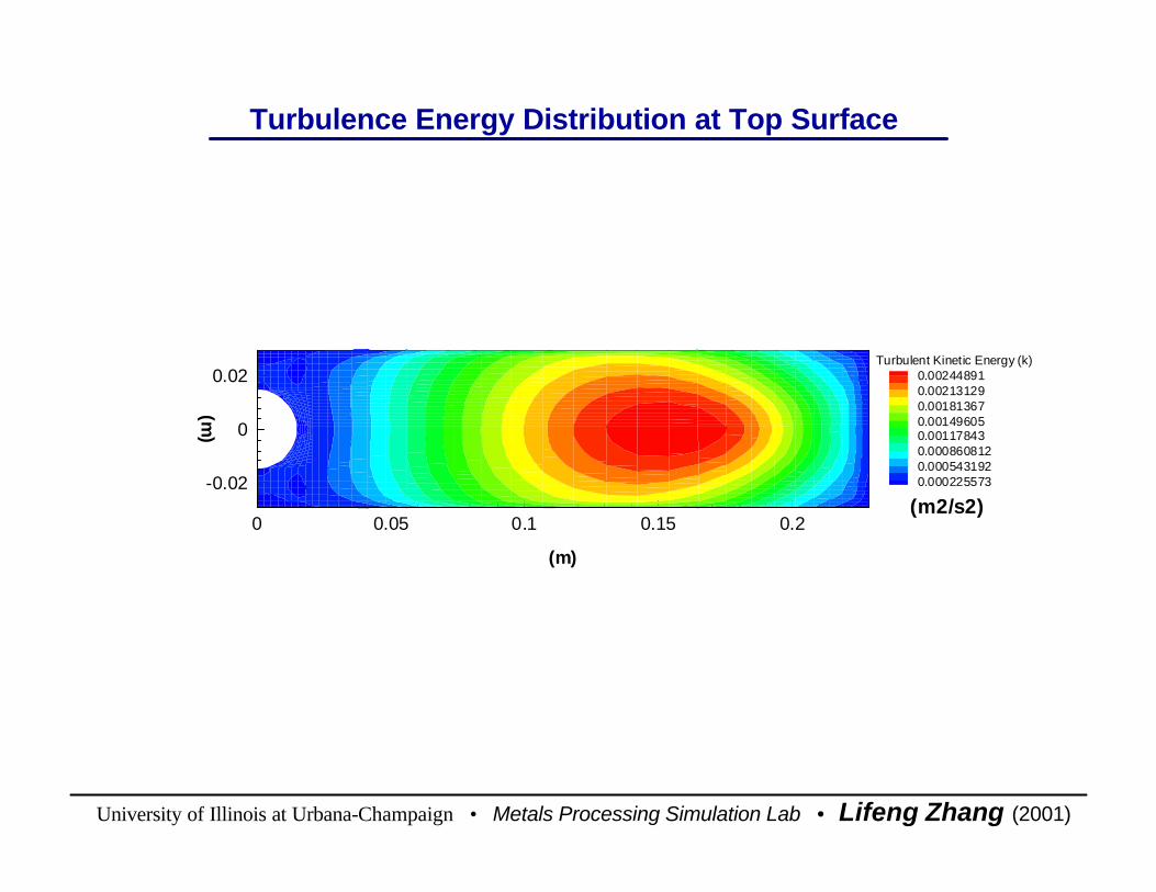
Turbulence Energy Distribution at Top SurfaceTurbulence Energy Distribution at Top Surface
-0.02
0
0.02
(m)
0 0.05 0.1 0.15 0.2
(m)
Turbulent Kinetic Energy (k)0.002448910.002131290.001813670.001496050.001178430.0008608120.0005431920.000225573
(m2/s2)

University of Illinois at Urbana-Champaign • Metals Processing Simulation Lab • Lifeng Zhang (2001)
Level Fluctuation Calculated from Turbulence Energy at Center Line along Width direction on Top Surface
Level Fluctuation Calculated from Turbulence Energy at Center Line along Width direction on Top Surface
( )gk
nFluctuatioLeveloilwater
water
ρρρ
−=
2
X. Huang, B.G.Thomas “Modeling Transient Flow Phenomena in Continuous Casting of Steel”, in 35th
Conference of Metallurgist, 23B, C. Twigge-Molecey eds, (Montreal, Canada: CIM, 1996), 339-356
X. Huang, B.G.Thomas “Modeling Transient Flow Phenomena in Continuous Casting of Steel”, in 35th
Conference of Metallurgist, 23B, C. Twigge-Molecey eds, (Montreal, Canada: CIM, 1996), 339-356
0.00 0.05 0.10 0.15 0.20 0.25
0.0000
0.0005
0.0010
0.0015
0.0020
0.0025
0.0030
k (m
2 /s2 )
mold half width (m)
0.00 0.05 0.10 0.15 0.20 0.250
1
2
3
4
5
6
7
water: 1000kg/m3
oil: 918 kg/m3
leve
l flu
ctua
tion
(mm
)
mold half width (m)

University of Illinois at Urbana-Champaign • Metals Processing Simulation Lab • Lifeng Zhang (2001)
Velocity, Pressure, Turbulent Energy at Top Surface for the Former Liquid Steel System
Velocity, Pressure, Turbulent Energy at Top Surface for the Former Liquid Steel System
0 0 .2 0.4 0.6 0.8
Mold half width (m)
-0.1
0
0.1Mold
thickness(m
)
0.4 00.3 50.3 00.2 50.2 00.1 50.1 00.0 50.0 0
1m/s
Speed (m/s)
0 0 .2 0.4 0.6 0.8
Mold half width (m)
-0.1
0
0.1
Mo
ldth
ickness
(m)
199.70129.67
59.63-10.41-80.44
-150.48-220.52-290.55-360.59
Gauge Pressure (pascal)
0 0 .2 0.4 0.6 0.8
Mold half width (m)
-0.1
0
0.1
Mold
thickness
(m)
0.001 870.001 670.001 470.001 270.001 070.000 870.000 670.000 470.000 27
Turbulent Energy (m2/s2)
University of Illinois at Urbana-Champaign • Metals Processing Simulation Lab • Lifeng Zhang (2001)
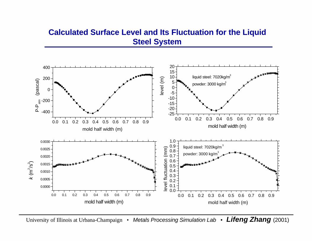
Calculated Surface Level and Its Fluctuation for the Liquid Steel System
Calculated Surface Level and Its Fluctuation for the Liquid Steel System
0.0 0.1 0.2 0.3 0.4 0.5 0.6 0.7 0.8 0.9-25-20-15-10-505
101520
liquid steel: 7020kg/m3
powder: 3000 kg/m3
leve
l (m
)
mold half width (m)
0.0 0.1 0.2 0.3 0.4 0.5 0.6 0.7 0.8 0.90.00.10.20.30.40.50.60.70.80.91.0
liquid steel: 7020kg/m 3
powder: 3000 kg/m3
leve
l flu
ctua
tion
(mm
)
mold half width (m)
0.0 0.1 0.2 0.3 0.4 0.5 0.6 0.7 0.8 0.9
0.0000
0.0005
0.0010
0.0015
0.0020
0.0025
0.0030
k (m
2 /s2 )
mold half width (m)
0.0 0.1 0.2 0.3 0.4 0.5 0.6 0.7 0.8 0.9
-400
-200
0
200
400
P-P
atm
(pas
cal)
mold half width (m)

University of Illinois at Urbana-Champaign • Metals Processing Simulation Lab • Lifeng Zhang (2001)
Velocity, Turbulence Energy and Its Dissipation Rate for a Full-Developed
Pipe Flow
Velocity, Turbulence Energy and Its Dissipation Rate for a Full-Developed
Pipe Flow

University of Illinois at Urbana-Champaign • Metals Processing Simulation Lab • Lifeng Zhang (2001)
uurr
xxRR
Velocity Distribution along Radial Direction[1]Velocity Distribution along Radial Direction[1]
n
Rr
uu
1
max1
−=
084.0Re81.2=n
( )( )xx u
nnnu 2max,
2121 ++=
νDu
=Re
u: velocity in x axial direction
umax: maximum value of u
Re: Reynolds number
R: radius of pipe
u: average velocity along radial direction
n: power of velocity distribution
r: distance along radial direction
u: velocity in x axial direction
umax: maximum value of u
Re: Reynolds number
R: radius of pipe
u: average velocity along radial direction
n: power of velocity distribution
r: distance along radial direction
[ 1] H. Schlichting . Boundary-Layer Theory, 1979, 7th ed., p599[ 1] H. Schlichting . Boundary-Layer Theory, 1979, 7th ed., p599

University of Illinois at Urbana-Champaign • Metals Processing Simulation Lab • Lifeng Zhang (2001)
[1] Bin Zhao’s LES simulation[2] J. G. M. Eggels et al. J. Fluid Mech. (1994), Vol.268, pp175-209[3] H. Schlichting. Boundary-Layer Theory, 1979, 7th ed., p599
[1] Bin Zhao’s LES simulation[2] J. G. M. Eggels et al. J. Fluid Mech. (1994), Vol.268, pp175-209[3] H. Schlichting. Boundary-Layer Theory, 1979, 7th ed., p599
Velocity Distribution along Radial DirectionVelocity Distribution along Radial Direction
0.0 0.2 0.4 0.6 0.8 1.0
0.0
0.2
0.4
0.6
0.8
1.0
LES, Re=5400 [1] DNS, Re=5300 [2] Schlichting's equation, Re=5400 [3]
u/u m
ax
r/R
University of Illinois at Urbana-Champaign • Metals Processing Simulation Lab • Lifeng Zhang (2001)
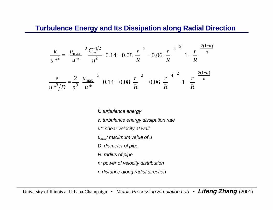
Turbulence Energy and Its Dissipation along Radial DirectionTurbulence Energy and Its Dissipation along Radial Direction
nn
Rr
Rr
Rr
n
C
uu
uk
)1(2242
2
212max
2 106.008.014.0**
−−
−
−
−
= µ
k: turbulence energy
ε: turbulence energy dissipation rate
u*: shear velocity at wall
umax: maximum value of u
D: diameter of pipe
R: radius of pipe
n: power of velocity distribution
r: distance along radial direction
k: turbulence energy
ε: turbulence energy dissipation rate
u*: shear velocity at wall
umax: maximum value of u
D: diameter of pipe
R: radius of pipe
n: power of velocity distribution
r: distance along radial direction
nn
Rr
Rr
Rr
uu
nDu
)1(32423max
33 106.008.014.0*
2*
−
−
−
−
=
ε

University of Illinois at Urbana-Champaign • Metals Processing Simulation Lab • Lifeng Zhang (2001)
[1] Bin Zhao’s LES simulation[2] J. G. M. Eggels et al. J. Fluid Mech. (1994), Vol.268, pp175-209[1] Bin Zhao’s LES simulation[2] J. G. M. Eggels et al. J. Fluid Mech. (1994), Vol.268, pp175-209
Turbulence Energy Distribution along Radial DirectionTurbulence Energy Distribution along Radial Direction
0.0 0.2 0.4 0.6 0.8 1.0
0
1
2
3
4
5
LES, Re=5400 [1] DNS, Re=5300 [2] Lifeng's equation (k-ε), Re=5400
k/u*
2
r/R

University of Illinois at Urbana-Champaign • Metals Processing Simulation Lab • Lifeng Zhang (2001)
1. For the fluid flow calculation in a full scale water model, uniform inlet k-εunderpredicts velocity peaks. With non-uniform inlet condition, all of k-ε, RSM and LES turbulence models have good agreement with experiment measurement. However, RSM model has slightly better prediction at some places, and k-ε model takes least time consuming.
2. For the particle motion, random walk model is better than streamline model because considering the effect of turbulence fluctuation.
3. It is concluded that entrapment of inclusions to walls has very strong effect to inclusion removal. The suitable entrapment model needs further development.
4. For the particle motion in full scale water model, RSM model has a best prediction of particle removal fraction compared to the experimental results. LES model overpredicts and k-ε far underpredicts.
Conclusions

University of Illinois at Urbana-Champaign • Metals Processing Simulation Lab • Lifeng Zhang (2001)
5. From the calculation of inclusion removal in steel caster (k-ε , random walk and without consideration of entrapment to walls), with increasing size, inclusion removal to the top surface becomes easier. Inclusions require about 10min to leave the domain of mold region (4m), and the total removal fraction to top surface is 63%, escape fraction to open bottom is 37%. After t=270s, inclusions removal to top surface becomes less than 0.5%.
6. The difference of particle removal fraction in water and liquid steel shows that the Stokes rising velocity is not a reasonable criterion for matching the particle behavior in water with inclusion behavior in liquid steel.
7. The top surface level and its fluctuation can be approximately estimated from the calculated pressure distribution for the flat top surface.
8. The developed models for the velocity and turbulence energy distribution for a full-developed pipe flow agree well with LES and DNS simulation.
Conclusions
University of Illinois at Urbana-Champaign • Metals Processing Simulation Lab • Lifeng Zhang (2001)
Further Investigations
1 The transient fluid flow simulation for the steel caster mold.
2 The suitable entrapment model of inclusion to the solidified shell.
3 The inclusions collision and coagulation simulation and its contribution to inclusion size growth and removal.
4 The interaction between inclusions and bubbles and its contribution to inclusion motion (removal) from mold.


