
Heywoodcases
StasKolenikov
Heywoodcases
Constrained?
Misspecified?
FactorHeywoodcases
References
Inference with Heywood cases
Stas Kolenikov
Joint work with Kenneth Bollen (UNC) and Victoria Savalei (UBC)NSF support from SES-0617193 with funds from SSA
September 18, 2009

Heywoodcases
StasKolenikov
Heywoodcases
Constrained?
Misspecified?
FactorHeywoodcases
References
What is a Heywood case?Heywood (1931) considered characterization of thecorrelation matrices:
1 r1r2 r1r3 . . . r1rn
r1r2 1 r2r3 . . . r2rn...
......
. . ....
r1rn r2rn r3rn . . . 1
, r1 ≥ r2 ≥ . . . ≥ rn ≥ 0
He showed that for this scheme
r21 ≤ 1 +
1r22
1−r22
+r23
1−r23
+ · · · r2n
1−r2n
and hence r1 can be greater than 1, which was an extensionon the earlier results by Spearman and Garnett.
Heywoodcases
StasKolenikov
Heywoodcases
Constrained?
Misspecified?
FactorHeywoodcases
References
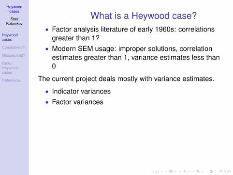
What is a Heywood case?• Factor analysis literature of early 1960s: correlations
greater than 1?• Modern SEM usage: improper solutions, correlation
estimates greater than 1, variance estimates less than0
The current project deals mostly with variance estimates.
• Indicator variances• Factor variances

Heywoodcases
StasKolenikov
Heywoodcases
Constrained?
Misspecified?
FactorHeywoodcases
References
Causes of Heywood cases• Outliers (Bollen 1987).• Non-convergence and underidentification (Van
Driel 1978, Boomsma & Hoogland 2001).• Empirical underidentification (Rindskopf 1984).• Structurally misspecified models (Van
Driel 1978, Dillon, Kumar &Mulani 1987, Sato 1987, Bollen 1989, Kolenikov &Bollen 2008).
• Sampling fluctuations (VanDriel 1978, Boomsma 1983, Anderson &Gerbing 1984).

Heywoodcases
StasKolenikov
Heywoodcases
Constrained?
Misspecified?
FactorHeywoodcases
References
Typology of Heywood casesInference problem:
H+ : σ2 > 0 “Normal” situation
H∅ : σ2 = 0 Perfect indicator (!?) or no factor present
H− : σ2 < 0 Misspecified model
Sample estimatePopulation value σ2 > 0 σ2 < 0σ2 > 0 , ??σ2 = 0 , ??σ2 < 0 Type I error Misspecification detected!

Heywoodcases
StasKolenikov
Heywoodcases
Constrained?
Misspecified?
FactorHeywoodcases
References
Breakdown of the papersSavalei & Kolenikov (2008)• Heywood case with an error variance.• True situation is H∅.• Should we consider H+ or H+ ∪ H− as an alternative?
Kolenikov & Bollen (2008)• Heywood case with an error variance.• True situation is H−; the model is structurally
misspecified.• Does it cause problems for inference?
Work in progress with Vika• Heywood case with an factor variance.• True situation is H∅, and there are even more serious
regularity condition violations.• Does it cause problems for inference?

Heywoodcases
StasKolenikov
Heywoodcases
Constrained?
Misspecified?
FactorHeywoodcases
References
Is that really a variance?
y1 y2 y3
ξ1
δ1 δ2 δ3
〈1〉
.
1
σ11 = λ21 + θ1
σ12 = λ1λ2σ13 = λ1λ3σ22 = λ2
2 + θ2σ23 = λ2λ3σ33 = λ2
3 + θ3

Heywoodcases
StasKolenikov
Heywoodcases
Constrained?
Misspecified?
FactorHeywoodcases
References
Is that really a variance?
y1 y2 y3
ξ1
δ1 δ2 δ3
〈1〉
.
1
λ1 =√
s12s13/s23
λ2 =√
s12s23/s13
λ3 =√
s13s23/s12
θ1 = s11 − s12s13/s23
θ2 = s22 − s12s23/s13
θ3 = s33 − s13s23/s12
Questions?

Heywoodcases
StasKolenikov
Heywoodcases
Constrained?
Misspecified?
FactorHeywoodcases
References
Savalei and Kolenikov (2008)Savalei, V. and Kolenikov, S. (2008), ‘Constrained vs.unconstrained estimation in structural equation modeling’,Psychological Methods 13, 150–170.
Research question: if the truth is H∅, should we test againstH+ or against H− ∪ H+?

Heywoodcases
StasKolenikov
Heywoodcases
Constrained?
Misspecified?
FactorHeywoodcases
References
Constrained estimation• Irregular problem: the standard regularity condition of interior
point is violated.
• Chernoff (1954): test with normal data of µ = 0 vs. µ > 0.
• Shapiro (1985): geometry of constrained parameter spacesin SEM.
• Stram & Lee (1994): variance components in mixed models.
• Jamshidian & Bentler (1994): algorithms for constrainedestimation for SEM.
• Andrews (1999, 2001) established the most general results.
• Stoel, Garre, Dolan & van den Wittenboer (2006):computational procedure for testing H∅ vs. H+.

Heywoodcases
StasKolenikov
Heywoodcases
Constrained?
Misspecified?
FactorHeywoodcases
References
Constrained estimationIf there are k parameters and r boundaries present, the(asymptotic) distribution is
T ∼k∑
j=k−r
wjχ2j , where
k∑j=k−r
wj = 1
with weights wj that depend on information matrix, i.e.,covariances between parameters.
Heywoodcases
StasKolenikov
Heywoodcases
Constrained?
Misspecified?
FactorHeywoodcases
References
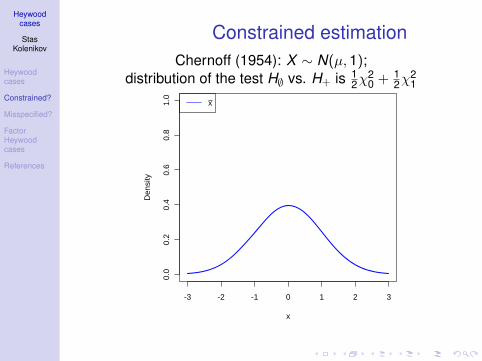
Constrained estimationChernoff (1954): X ∼ N(µ,1);
distribution of the test H∅ vs. H+ is 12χ
20 + 1
2χ21
-3 -2 -1 0 1 2 3
0.0
0.2
0.4
0.6
0.8
1.0
x
Den
sity
x

Heywoodcases
StasKolenikov
Heywoodcases
Constrained?
Misspecified?
FactorHeywoodcases
References
Constrained estimationChernoff (1954): X ∼ N(µ,1);
distribution of the test H∅ vs. H+ is 12χ
20 + 1
2χ21
-3 -2 -1 0 1 2 3
0.0
0.2
0.4
0.6
0.8
1.0
x
Den
sity
xμ

Heywoodcases
StasKolenikov
Heywoodcases
Constrained?
Misspecified?
FactorHeywoodcases
References
Constrained estimationChernoff (1954): X ∼ N(µ,1);
distribution of the test H∅ vs. H+ is 12χ
20 + 1
2χ21
-3 -2 -1 0 1 2 3
0.0
0.2
0.4
0.6
0.8
1.0
x
Den
sity
x

Heywoodcases
StasKolenikov
Heywoodcases
Constrained?
Misspecified?
FactorHeywoodcases
References
Constrained estimationChernoff (1954): X ∼ N(µ,1);
distribution of the test H∅ vs. H+ is 12χ
20 + 1
2χ21
-3 -2 -1 0 1 2 3
0.0
0.2
0.4
0.6
0.8
1.0
x
Den
sity
xμ
Heywoodcases
StasKolenikov
Heywoodcases
Constrained?
Misspecified?
FactorHeywoodcases
References
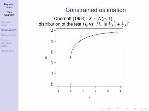
Constrained estimationChernoff (1954): X ∼ N(µ,1);
distribution of the test H∅ vs. H+ is 12χ
20 + 1
2χ21
-1 0 1 2 3 4
0.0
0.2
0.4
0.6
0.8
1.0
x
cdf

Heywoodcases
StasKolenikov
Heywoodcases
Constrained?
Misspecified?
FactorHeywoodcases
References
Constrained estimation: consSavalei & Kolenikov (2008):
• Mixtures arise only when a combination of conditions abouttrue parameters (unknown to the researcher) and estimationprocedures (constrained estimation) occur together.
• Test of overall fit has distribution which is impossible tocharacterize (due to unknowns). Conservative upper bound:χ2
k .
• Constrained estimation is only internally consistent when allthe procedures are laid out ahead rather than followed thedata!
• Ad hoc procedure of resetting Heywood cases to zero:effectively equivalent to constrained estimation, but type Ierror is likely inflated.
• Software implementation: explicit constraints are required; afar more difficult optimization procedure.
• Non-normal data and not asymptotically robust situations:just forget it.

Heywoodcases
StasKolenikov
Heywoodcases
Constrained?
Misspecified?
FactorHeywoodcases
References
Conditional approachDijkstra (1992): start with the first stage estimation; ifHeywood cases occur:
1 restrict parameter(s);2 release degree(s) of freedom;3 re-estimate the model and report p-value only. The test
statistic itself is not meaningful.In this conditional approach, the unconditional distribution isagain the mixture. It also leads to somewhat improved finitesample approximation when the parameter is near theboundary.Implementation: SAS PROC CALIS

Heywoodcases
StasKolenikov
Heywoodcases
Constrained?
Misspecified?
FactorHeywoodcases
References
Unconstrained estimationSavalei & Kolenikov (2008):• Overall fit test has a known distribution, same for all
points in parameter space!• Decomposition of χ2 into the fit and effect of the
boundary components.• Easier to implement than constrained estimation.• More informative about sources of misfit.• Provides power against a broader range of alternatives.

Heywoodcases
StasKolenikov
Heywoodcases
Constrained?
Misspecified?
FactorHeywoodcases
References
Software implementationSavalei & Kolenikov (2008) compared AMOS 7.0, EQS 6.1,LISREL 8.8, Mplus 4.2, and SAS PROC CALIS in SAS 9.1.
• Unconstrained estimation is default in all softwarepackages except EQS.
• Release one d.f. for conditional inference: only in SASPROC CALIS.
• Constrained Wald test: no software does that.• Numerical and conceptual discrepancies between
packages.• Convergence diagnostic/missing s.e. problems with
LISREL.• Should the standard error on the constrained
parameter be zero?• Factor correlations > 1: parameterization may matter.

Heywoodcases
StasKolenikov
Heywoodcases
Constrained?
Misspecified?
FactorHeywoodcases
References
Phantom variablesRindskopf (1983): device to impose inequality constraints.
the issue that is somewhat concealed when the focus is onmixtures: that in order to gain power on one tail of thedistribution we must explicitly ignore the other tail.
Constrained and Unconstrained Estimation inPopular SEM Software
As the SEM field is heavily software dependent, it iscrucial to know how different software packages treat Hey-wood cases and how, and whether, they implement con-straints. In this section, we compare constrained and uncon-strained estimation defaults and options in several popularSEM packages. We consider the following programs: Amos7.0 (Arbuckle, 2007), EQS 6.1 (Bentler, 2007), LISREL 8.8(Joreskog & Sorbom, 1997), Mplus 4.2 (Muthen & Muthen,2006), and Proc Calis (available in SAS 9.1).8 These werethe latest versions at the time of writing.
First, however, we briefly discuss two alternative ways ofmimicking constrained estimation that do not require spec-ifying inequality constraints via the software: the ad hocapproach and the model reparameterization approach. Thesealternative approaches are often used (e.g., Stoel et al.,2006, relied on them exclusively), and they are sometimesperceived to be equivalent to software implementation. Wedo not recommend these approaches. The ad hoc approachproceeds as follows: Fit a model, observe any inadmissibleestimates, and rerun the model with offending estimatesfixed to their boundary values. This approach is less thanideal. First, it may require iteration: Constraining one of-fending estimate to the boundary value may produce an-other offending estimate, and so on. Second, this approachwill produce the correct solution when the likelihood sur-face is quadratic, so that a unique global optimizer exists. Inthis case, the simplified picture of the restricted surfacelooks much like Figure 1, and stopping at the boundary
gives the right solution (Dijkstra, 1992). But in smallersamples and with larger models, the likelihood surface maybehave much worse and have a weird shape and multiplelocal maxima; at what point this is no longer a concern isnot clear (Bentler & Tanaka, 1983; Dillon et al., 1987;Loken, 2005; Rubin & Thayer, 1982). An additional disad-vantage of the ad hoc approach is that it allows researchersto see the inadmissible estimates and their standard errors.This makes it difficult to disregard this information, yet thisis precisely what is required to carry out constrained esti-mation correctly, as we discuss later.
The approach of reparameterization was proposed byRindskopf (1983, 1984) as a way to impose inequalityconstraints at the time when SEM software packages did notallow for them (see also Bentler, 1976; Dillon et al., 1987).He suggested, for example, that to keep residual variancesfrom going negative, the variances of the error terms can befixed to 1 and their regression coefficients estimated instead.Figure 4 illustrates how a standard growth-curve model canbe reparameterized to avoid negative estimates of the vari-ance of the slope factor by the introduction of a phantomvariable V (Rindskopf, 1983, 1984). Writing S bV, wehave that var(S) b2, and the estimated slope variance isalways nonnegative, regardless of the value of b. However,this approach will run into trouble when the estimated valueof b is zero or near zero—which is precisely the situation weare interested in here—as in that case the derivatives matrixfor the model is singular or near-singular. Appendix Bdemonstrates this. Additionally, the seemingly attractiveproperty of this approach, namely, that it obviates the needfor inequality constraints, is also its shortcoming, in that theresearcher will be less likely to be reminded of the fact thatthe implicit inequality constraints may be affecting thedistribution of the test statistic. As Rindskopf (1984) noted,“it would be preferable to be able to make a direct statementof the desired constraints, and let the computer programimplement them, instead of using ‘tricks’” (p. 46).
Most commercially available SEM software packagesnow allow users to impose at least linear inequality con-straints. Of the five programs we considered, all but Amos7.0 allow such constraints. EQS 6.1 is the only program thatrestricts residual variances to be positive by default;9 it alsorestricts latent correlations from exceeding 1 wheneveridentification is done by fixing factor variances. Appendix C
8 This list is by no means exhaustive, and other programs exist(e.g., Mx, RAMONA, the sem package in R, the gllamm packagein Stata). We picked what we perceived to be the five most popularcommercially available packages.
9 Constrained estimation is often the default in programs forother types of latent variable models, for example, the Proc Mixedprocedure in SAS, which fits random effects models. We do notstudy these programs here, but our discussion of the behavior ofthe test statistic under constraints applies to these models as well.
I
Y1 Y4Y3Y2
-7 13
3
S
1111
b
V
Figure 4. A parameterization of a standard growth curve modelto create an implicit inequality constraint on the variance of the slopefactor. Variance of V is fixed to 1. I intercept factor; S slopefactor; V phantom latent variable; Y1–Y4 observed variables.
158 SAVALEI AND KOLENIKOV
• V[S] = ψS = b2
• When ψS = 0, b = 0, and ∂l/∂ψS = 2b · ∂l/∂b = 0, soinformation matrix is not invertible!
• Phantom variables substitute one irregularity foranother.

Heywoodcases
StasKolenikov
Heywoodcases
Constrained?
Misspecified?
FactorHeywoodcases
References
Recommended procedures• Commit to restricting the estimates to be in their proper
range; use conditional approach to overall fit test andmixture distribution for χ2 difference tests.
• Leave the choice to the software and don’t intervene(EQS: constrained estimation)
• Allow inadmissible solutions and test them forsignificance. Use Wald tests, confidence intervals or χ2
difference tests that all have their “regular” distributions.
Questions?

Heywoodcases
StasKolenikov
Heywoodcases
Constrained?
Misspecified?
FactorHeywoodcases
References
Kolenikov and Bollen (2008)Kolenikov, S. and Bollen, K. A. (2008), ‘Testing negativeerror variances: Is a Heywood case a symptom ofmisspecification?’ Under review.
Research question: testing specification, as expressed via
H∅ ∪ H+ against H−

Heywoodcases
StasKolenikov
Heywoodcases
Constrained?
Misspecified?
FactorHeywoodcases
References
Population Heywood caseData generating process
〈1〉
y1
y2
y3
ζ2〈1〉
ζ3〈1〉
0.3
0.55
0.8
.
1
Jump to simulations

Heywoodcases
StasKolenikov
Heywoodcases
Constrained?
Misspecified?
FactorHeywoodcases
References
Population Heywood caseCFA model fit
y1 y2 y3
ξ1
δ1 δ2 δ3
〈0.229〉
11.313
3.457
〈0.771〉 〈0.696〉 〈−0.467〉
.
1
Jump to simulations

Heywoodcases
StasKolenikov
Heywoodcases
Constrained?
Misspecified?
FactorHeywoodcases
References
Population Heywood caseCFA with restricted variance
y1 y2 y3
ξ1
δ1 δ2 δ3
〈0.275〉
11.313
2.866
〈0.724〉 〈0.615〉 〈0〉
.
1
Jump to simulations

Heywoodcases
StasKolenikov
Heywoodcases
Constrained?
Misspecified?
FactorHeywoodcases
References
Misspecified models• Distributional misspecification: the distribution of the
data is not normal, likelihood methods are not fullyapplicable (Satorra 1990, Satorra & Bentler 1994).
• Structural misspecification: the structure of the model,the number of latent variables, the relations betweenthe variables in the model are not specified correctly(Yuan, Marshall & Bentler 2003).
• Heywood case: impossible value in the population;evidence of structural misspecification (or what??)
• If the model is misspecified, doesn’t everything just fallapart??

Heywoodcases
StasKolenikov
Heywoodcases
Constrained?
Misspecified?
FactorHeywoodcases
References
Misspecified models• Huber (1967)
• Point estimates are consistent for the minimizer of thepopulation fit function:
arg min F (S,Σ(θ))→ arg min F (Σ,Σ(θ)) ≥ 0,
F (Ω,Σ(θ)) = ln |Σ(θ)|+ Σ(θ)−1Ω− ln |S| − dim Σ(θ) =as.eq.
= (ω − σ(θ))′ V (ω − σ(θ)),
ω = vech Ω, σ(θ) = vech Σ(θ)
• Uncertainty about these estimates is given by anasymptotic covariance matrix (sandwich estimator):
√n(θn − θ0)
d−→ N(0,A−1BA−T ),
A = E ∂ψ(X , θ0), B = Eψ(X , θ0)ψ(X , θ0)T ,
ψ(X , θ0) = −σ(θ)′V (s − σ(θ))

Heywoodcases
StasKolenikov
Heywoodcases
Constrained?
Misspecified?
FactorHeywoodcases
References
Misspecified modelsSpecial cases:
• Eicker (1967) and White (1980), linear regression withheteroskedastic errors:
β = (X ′X )−1X ′y , v(β) = (X ′X )−1(X ′ee′X )(X ′X )−1
• Browne (1974): least squares estimator for SEM.
• White (1982): somewhat milder regularity conditions that areeasier to check in practice; application to some commoneconometric models.
• Arminger & Schoenberg (1989): an econometrics paper inPsychometrika.
• Satorra & Bentler (1994): model based sandwich estimatorwith explicit expression for matrix B (the meat of thesandwich) as a function of the model parameters and thefourth order moments of data.
• Yuan & Hayashi (2006): comparison of empirical sandwichand the bootstrap standard errors for SEM.

Heywoodcases
StasKolenikov
Heywoodcases
Constrained?
Misspecified?
FactorHeywoodcases
References
Can standard errors be trusted?
Distributional Structural specificationspecification Correct Incorrect
Correct I, S-B, ES, EB, BSB I, ES, EBIncorrect S-B, ES, EB, BSB ES, EB
Analytic standard errors:I observed or expected information matrix
S-B Satorra-Bentler standard errorsES empirical (Huber) sandwich
Resampling standard errors:
EB empirical bootstrapBSB Bollen-Stine bootstrap with data rotation
Heywoodcases
StasKolenikov
Heywoodcases
Constrained?
Misspecified?
FactorHeywoodcases
References
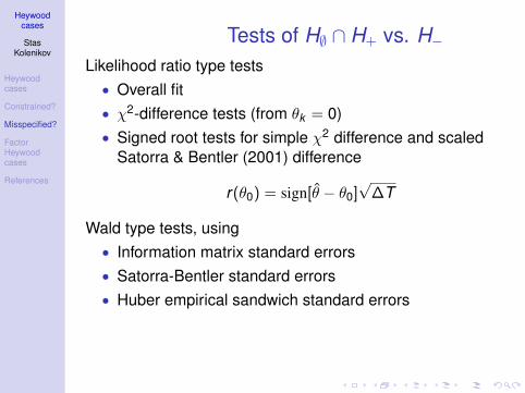
Tests of H∅ ∩ H+ vs. H−Likelihood ratio type tests• Overall fit• χ2-difference tests (from θk = 0)• Signed root tests for simple χ2 difference and scaled
Satorra & Bentler (2001) difference
r(θ0) = sign[θ − θ0]√
∆T
Wald type tests, using• Information matrix standard errors• Satorra-Bentler standard errors• Huber empirical sandwich standard errors

Heywoodcases
StasKolenikov
Heywoodcases
Constrained?
Misspecified?
FactorHeywoodcases
References
Simulation studySaturated model with 3 variables and 6 parameters: χ2
0 ≡ 0,no way to test the model fit. . . unless you hit a Heywoodcase!
Jump to the Heywood case in population example
Main results:• HUGE biases of the Heywood case in small samples.• Information matrix standard errors are biased leading to
undercoverage of CIs based on them when the dataare non-normal.

Heywoodcases
StasKolenikov
Heywoodcases
Constrained?
Misspecified?
FactorHeywoodcases
References
Simulation studyLarger model with 4 variables, 8 parameters and 2 d.f. for modelfit test.Data generating process
y3
y1
〈1〉
y2
y4
ζ2 〈1〉
ζ3 〈1〉 ζ4 〈1〉
0.8
−0.1
0.4
−0.1
0.6
.
1

Heywoodcases
StasKolenikov
Heywoodcases
Constrained?
Misspecified?
FactorHeywoodcases
References
Simulation studyLarger model with 4 variables, 8 parameters and 2 d.f. for modelfit test.CFA model fit
y1 y2 y3 y4
ξ1
δ1 δ2 δ3 δ4
〈1.195〉
10.345 0.633
0.464
〈−0.195〉 〈1.018〉 〈1.109〉 〈1.066〉
.
1

Heywoodcases
StasKolenikov
Heywoodcases
Constrained?
Misspecified?
FactorHeywoodcases
References
Simulation studyLarger model with 4 variables, 8 parameters and 2 d.f. for modelfit test.CFA with restricted variance
y1 y2 y3 y4
ξ1
δ1 δ2 δ3 δ4
〈1〉
10.4 0.76
0.56
〈0〉 〈1〉 〈1.01〉 〈1.01〉
.
1
Heywoodcases
StasKolenikov
Heywoodcases
Constrained?
Misspecified?
FactorHeywoodcases
References
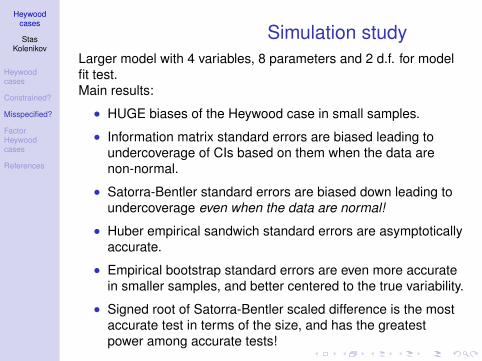
Simulation studyLarger model with 4 variables, 8 parameters and 2 d.f. for modelfit test.Main results:
• HUGE biases of the Heywood case in small samples.
• Information matrix standard errors are biased leading toundercoverage of CIs based on them when the data arenon-normal.
• Satorra-Bentler standard errors are biased down leading toundercoverage even when the data are normal!
• Huber empirical sandwich standard errors are asymptoticallyaccurate.
• Empirical bootstrap standard errors are even more accuratein smaller samples, and better centered to the true variability.
• Signed root of Satorra-Bentler scaled difference is the mostaccurate test in terms of the size, and has the greatestpower among accurate tests!

Heywoodcases
StasKolenikov
Heywoodcases
Constrained?
Misspecified?
FactorHeywoodcases
References
Zero factor variancesKoleinkov and Savalei: work in progress.Question: testing factor variances, as opposed to errorvariances.
Factor 1
x1
1
x2 x3 x4
Factor 2
x5
1
x6 x7 x8
Method 1
1
Method2
1

Heywoodcases
StasKolenikov
Heywoodcases
Constrained?
Misspecified?
FactorHeywoodcases
References
Zero factor variancesKoleinkov and Savalei: work in progress.Question: testing factor variances, as opposed to errorvariances.Complications:• If a factor variance is zero, what happens to its
covariances with other factors and the loadings ofobserved variables?
• How many parameters are we actually testing?• What are degrees of freedom?

Heywoodcases
StasKolenikov
Heywoodcases
Constrained?
Misspecified?
FactorHeywoodcases
References
Zero factor variancesTechnically speaking, zero factor variances lead tounderidentified models.
φk = 0⇒ Corr(ξk , ξj) is underID, λlk is underID
Technical research into underidentified models(Davies 1977, Davies 1987, Andrews &Ploberger 1994, Hansen 1996):• Asymptotic distribution still exists!• It is characterized by maxχ2(θ) over a range of θ• Analytical work is very limited• Simulation approach seem attractive

Heywoodcases
StasKolenikov
Heywoodcases
Constrained?
Misspecified?
FactorHeywoodcases
References
Simulation study• Data generation: 1 factor multivariate normal model, 6
variables.• Fitted models: extra one or two factors, loading on half
of the variables each.
Factor
x1
1
x2 x3 x4 x5 x6
Method 1
1
Method 2
1
• Numeric stability issues: hundreds of maximizationiterations; ridge-like likelihoods; absurd parameterestimates and standard errors.
Heywoodcases
StasKolenikov
Heywoodcases
Constrained?
Misspecified?
FactorHeywoodcases
References
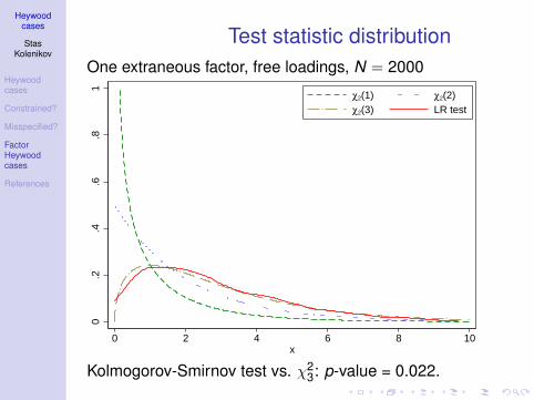
Test statistic distributionOne extraneous factor, free loadings, N = 2000
0.2
.4.6
.81
0 2 4 6 8 10x
χ2(1) χ2(2)χ2(3) LR test
Kolmogorov-Smirnov test vs. χ23: p-value = 0.022.

Heywoodcases
StasKolenikov
Heywoodcases
Constrained?
Misspecified?
FactorHeywoodcases
References
Test statistic distributionOne extraneous factor, fixed loadings, N = 2000
0.2
.4.6
.81
0 2 4 6 8 10x
χ2(1) χ2(2)χ2(3) LR test
Kolmogorov-Smirnov test vs. χ21: p-value = 0.115.
Heywoodcases
StasKolenikov
Heywoodcases
Constrained?
Misspecified?
FactorHeywoodcases
References
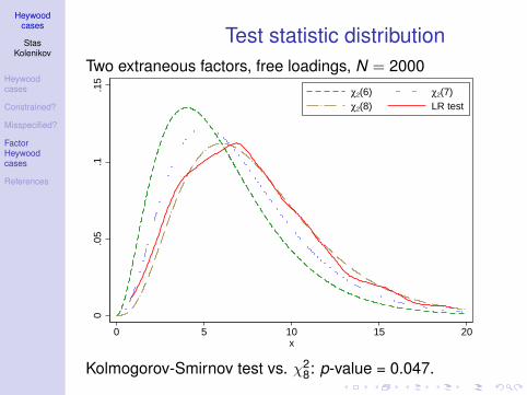
Test statistic distributionTwo extraneous factors, free loadings, N = 2000
0.0
5.1
.15
0 5 10 15 20x
χ2(6) χ2(7)χ2(8) LR test
Kolmogorov-Smirnov test vs. χ28: p-value = 0.047.

Heywoodcases
StasKolenikov
Heywoodcases
Constrained?
Misspecified?
FactorHeywoodcases
References
References IAnderson, J. C. & Gerbing, D. (1984), ‘The effect of sampling error on
convergence, improper solutions, and goodness-of-fit indices formaximum likelihood confirmatory factor analysis’, Psychometrika49, 155–173.
Andrews, D. W. K. (1999), ‘Estimation when a parameter is on aboundary’, Econometrica 67(6), 1341–1383.
Andrews, D. W. K. (2001), ‘Testing when a parameter is on the boundaryof the maintained hypothesis’, Econometrica 69(3), 683–734.doi:10.1111/1468-0262.00210.
Andrews, D. W. K. & Ploberger, W. (1994), ‘Optimal tests when anuisance parameter is present only under the alternative’,Econometrica 62(6), 1383–1414.
Arminger, G. & Schoenberg, R. J. (1989), ‘Pseudo maximum likelihoodestimation and a test for misspecification in mean and covariancestructure models’, Psychometrika 54, 409–426.
Bollen, K. A. (1987), ‘Outliers and improper solutions: A confirmatoryfactor analysis example’, Sociological Methods and Research15, 375–384.

Heywoodcases
StasKolenikov
Heywoodcases
Constrained?
Misspecified?
FactorHeywoodcases
References
References IIBollen, K. A. (1989), Structural Equations with Latent Variables, Wiley,
New York.Boomsma, A. (1983), On the Robustness of LISREL (Maximum
Likelihood Estimation) Against Small Sample Size andNonnormality, Sociometric Research Foundation, Amsterdam, theNetherlands.
Boomsma, A. & Hoogland, J. J. (2001), ‘The robustness of LISRELmodeling revisited’, Structural Equation Modeling: Present andFuture.
Browne, M. W. (1974), ‘Generalized least squares estimators in theanalysis of covariances structures’, South African Statistical Journal8, 1–24.
Chernoff, H. (1954), ‘On the distribution of the likelihood ratio’, TheAnnals of Mathematical Statistics 25(3), 573–578.
Davies, R. B. (1977), ‘Hypothesis testing when a nuisance parameter ispresent only under the alternative’, Biometrika 64(2), 247–254.
Davies, R. B. (1987), ‘Hypothesis testing when a nuisance parameter ispresent only under the alternatives’, Biometrika 74(1), 33–43.

Heywoodcases
StasKolenikov
Heywoodcases
Constrained?
Misspecified?
FactorHeywoodcases
References
References IIIDijkstra, T. K. (1992), ‘On statistical inference with parameter estimates
on the boundary of the parameter space’, British Journal ofMathematical and Statistical Psychology 45, 289–309.
Dillon, W. R., Kumar, A. & Mulani, N. (1987), ‘Offending estimates incovariance structure analysis: Comments on the causes andsolutions to Heywood cases’, Psychological Bulletin 101, 126–135.
Eicker, F. (1967), Limit theorems for regressions with unequal anddependent errors, in ‘Proceedings of the Fifth Berkeley Symposiumon Mathematical Statistics and Probability’, Vol. 1, University ofCalifornia Press, Berkeley, pp. 59–82.
Hansen, B. E. (1996), ‘Inference when a nuisance parameter is notidentified under the null hypothesis’, Econometrica 64(2), 413–430.
Heywood, H. B. (1931), ‘On finite sequences of real numbers’,Proceedings of the Royal Society of London. Series A, ContainingPapers of a Mathematical and Physical Character134(824), 486–501.
Heywoodcases
StasKolenikov
Heywoodcases
Constrained?
Misspecified?
FactorHeywoodcases
References
References IVHuber, P. (1967), The behavior of the maximum likelihood estimates
under nonstandard conditions, in ‘Proceedings of the Fifth BerkeleySymposium on Mathematical Statistics and Probability’, Vol. 1,University of California Press, Berkeley, pp. 221–233.
Jamshidian, M. & Bentler, P. M. (1994), ‘Gramian matrices in covariancestructure models’, Applied Psychological Measurement18(1), 79–94.
Kolenikov, S. & Bollen, K. A. (2008), Testing negative error variances: Isa Heywood case a symptom of misspecification? under review inSociological Methods and Research.
Rindskopf, D. (1983), ‘Parameterizing inequality constraints on uniquevariances in linear structural models’, Psychometrika 48(1), 73–83.
Rindskopf, D. (1984), ‘Structural equation models: Empiricalidentification, Heywood cases, and related problems’, SociologicalMethods and Research 13, 109–119.
Sato, M. (1987), ‘Pragmatic treatment of improper solutions in factoranalysis’, Annals of the Institute of Statistics and Mathematics, partB 39, 443–455.

Heywoodcases
StasKolenikov
Heywoodcases
Constrained?
Misspecified?
FactorHeywoodcases
References
References VSatorra, A. (1990), ‘Robustness issues in structural equation modeling: A
review of recent developments’, Quality and Quantity 24, 367–386.
Satorra, A. & Bentler, P. (2001), ‘A scaled difference chi-square teststatistic for moment structure analysis’, Psychometrika66(4), 507–514.
Satorra, A. & Bentler, P. M. (1994), Corrections to test statistics andstandard errors in covariance structure analysis, in A. von Eye &C. C. Clogg, eds, ‘Latent variables analysis’, Sage, ThousandsOaks, CA, pp. 399–419.
Savalei, V. & Kolenikov, S. (2008), ‘Constrained vs. unconstrainedestimation in structural equation modeling’, Psychological Methods13, 150–170.
Shapiro, A. (1985), ‘Asymptotic distribution of test statistic in the analysisof moment structures under inequality constraints’, Biometrika72(1), 133–144.

Heywoodcases
StasKolenikov
Heywoodcases
Constrained?
Misspecified?
FactorHeywoodcases
References
References VIStoel, R. D., Garre, F. G., Dolan, C. & van den Wittenboer, G. (2006), ‘On
the likelihood ratio test in structural equation modeling whenparameters are subject to boundary constraints’, PsychologicalMethods 11(4).
Stram, D. O. & Lee, J. W. (1994), ‘Variance components testing in thelongitudinal mixed effects model’, Biometrics 50(4), 1171–1177.
Van Driel, O. P. (1978), ‘On various causes of improper solutions inmaximum likelihood factor analysis’, Psychometrika 43, 225–43.
White, H. (1980), ‘A heteroskedasticity-consistent covariance-matrixestimator and a direct test for heteroskedasticity’, Econometrica48(4), 817–838.
White, H. (1982), ‘Maximum likelihood estimation of misspecifiedmodels’, Econometrica 50(1), 1–26.
Yuan, K.-H. & Hayashi, K. (2006), ‘Standard errors in covariancestructure models: Asymptotics versus bootstrap’, British Journal ofMathematical and Statistical Psychology 59, 397–417.

Heywoodcases
StasKolenikov
Heywoodcases
Constrained?
Misspecified?
FactorHeywoodcases
References
References VIIYuan, K. H., Marshall, L. L. & Bentler, P. M. (2003), ‘Assessing the effect
of model misspecifications on parameter estimates in structuralequation models’, Sociological Methodology 33(1), 241–265.


