

The South Africa I know, the home I understand
INTER-LINKAGES BETWEEN PRIVATE INVESTMENT,PUBLIC INVESTMENT AND ECONOMIC
GROWTH IN SOUTH AFRICA
Sagaren Pillay
ERAN: East London:March 2016

The South Africa I know, the home I understand
1. Introduction
2. Data matters
3. Methodology
4. Diagnostics
5. Conclusions
The South Africa I know, the home I understand
• Empirical research in macroeconomics as well as in financial economics is largely based on time series.
• Economic time series can be viewed as realizations of stochastic processes.
• Clive Granger has shown that macroeconomic models containing non-stationary stochastic variables can be constructed in such a way that the results are both statistically sound and economically meaningful.

The South Africa I know, the home I understand
• The cointegration relationship between private investment and public investment as well as the relationship between total investment and output has been researched extensively over the past decade. Government and Private spending-impact on economy
• Every rand of increased government spending-one less rand of private spending??
• Research exploring the short-run and long run linkages and dynamic interaction between the three variables, considered jointly is very limited.
• Policy makers need to understand the relationship between investment and economic growth and the interactions between them in order to improve macroeconomic performance.

The South Africa I know, the home I understand
• The objective of this paper is to explore the inter-linkages between private investment, public investment and economic growth in South Africa by using quarterly and annual data from 2005 to 2014.
• The theoretical framework for the study is based on Johansen’s cointegration approach and vector error correction modelling.

The South Africa I know, the home I understand
• The annual public expenditure data was temporally disaggregated to quarterly data. Numerical smoothing procedure.
• The SAS EXPAND procedure uses the SPLINE method by fitting a cubic spline curve to the input values.
• A cubic spline is a segmented function consisting of third-degree (cubic) polynomial functions joined together so that the whole curve and its first and second derivatives are continuous.
The South Africa I know, the home I understand
• Y1 = log GDP
• Y2 = log Private_Capex
• Y3 = log Public_Capex
• Y4 = log Total_Capex
The South Africa I know, the home I understand
UNIT ROOT TEST
• The first step in the time series analysis was to determine whether the two series are stationary or non-stationary in nature
• If the time series are I (1), they have to be characterized by the presence of a unit root and their first difference by the absence of unit roots (Hendry & Juselius, 2001).

The South Africa I know, the home I understand
• The Augmented Dickey Fuller (ADF) unit root test was used to determine whether the series was stationary or non-stationary.
• The Dickey- Fuller tests for non-stationarity of each of the series is shown below (Table 1)
• The null hypothesis is to test a unit root.
• Consequently, the series have a unit root. Thus, the variables are first order difference stationary.

The South Africa I know, the home I understand
Variable Type Rho Pr < Rho Tau Pr < Tau
y1 Zero Mean 0.06 0.6905 4.47 0.9999Single Mean -0.82 0.896 -1.69 0.4262Trend -11.2 0.2959 -2.48 0.3352
y2 Zero Mean 0.13 0.7051 1.65 0.9734Single Mean -7.15 0.2371 -2.62 0.0986Trend -14.76 0.1318 -3.26 0.0903
y3 Zero Mean 0.1 0.6995 0.64 0.85Single Mean -2.85 0.6608 -2 0.2843Trend -22.5 0.0149 -4.32 0.0083
y4 Zero Mean 0.12 0.7031 2.92 0.9987Single Mean -2.28 0.7335 -2.54 0.1148Trend -5.34 0.7745 -2.3 0.4211
Dickey-Fuller Unit Root Tests

The South Africa I know, the home I understand
• The null hypothesis is to test a unit root. In the Dickey-Fuller tests, the second column specifies three types of models, which are zero mean, single mean, or trend.
• The third column (Rho) and the fifth column (Tau) are the test statistics for unit root testing.
• Other columns are the p-values. Consequently, all series have a unit root and their first differences do not have any.
• Thus, the variables y1, y2 , y3 and y4 are first order difference stationary and are integrated, I (1) .

The South Africa I know, the home I understand
We consider a VAR(p) with xt I(1), (unit root) nonstationary
xt = ϕ + Φ1xt−1 + . . . + Φpxt−p + ϵt
Then
Δxt is I(0) and π = −Φ(1) is singular, i.e. |Φ(1)| = 0
The VEC representation reads with π = αβ′
Δxt = ϕ + πxt−1 + ΣΦ∗I Δxt−i + ϵt
Where
πxt−1 is called the error-correction term
An important characteristic of equilibrium –correction formulation is the inclusion of both differences and levels in the same model- allows us to investigate both short run and long run effects in the data.

The South Africa I know, the home I understand
• π = 0, the null matrix.
• There does not exist a linear combination of the I(1) vars,which is stationary.
• The x’s are not cointegrated.
• The EC form reduces to a stationary VAR(p − 1) in differences.
• π has m = 0 eigenvalues, which are not different from 0

The South Africa I know, the home I understand
• There are m linear independent cointegrating (column) vectors in β.
• The m stationary linear combinations are β′xt . xt has (k − m) unit roots, so (k − m) common stochastic trends.
• There are k I(1) variables, m cointegrating relations (eigenvalues of π different from 0), and I (k − m) stochastic trends.

The South Africa I know, the home I understand
Full rank of π implies
• that |π| = | − Φ(1)| <> 0.
• xt has no unit root. That is xt is I(0).
• There are (k − m) = 0 stochastic trends.
• As consequence we model the relationship of the x’s in levels, not in differences.
• There is no need to refer to the error correction representation.

The South Africa I know, the home I understand
H0 : π = -αβ΄
For any π there are infinitely many α, β such that
π = -αβ΄ since -αβ΄= - αTT-1 β΄ so we don’t test hypothesis about α and β, only about the
rank r (αT=A, T-1 β΄=B, α β΄ = π)

The South Africa I know, the home I understand
rank test:
H0 : Rank(π) = m against HA : Rank(π) > m
We start with m = 0 – that is Rank(π) = 0, there is no cointegration – against m ≥ 1, that there is at least one cointegratring relation.

The South Africa I know, the home I understand
• Cointegration between Public and Private investment expenditure (y2 and y3).
• The Johansen and Julius cointegration statistic test for testing the null hypothesis that there are at most r cointegrated vectors is used versus the alternative Hypothesis of more than r co integrated-vectors.
• An autoregressive order 3 was slected based on the minimum information criterion.
The South Africa I know, the home I understand
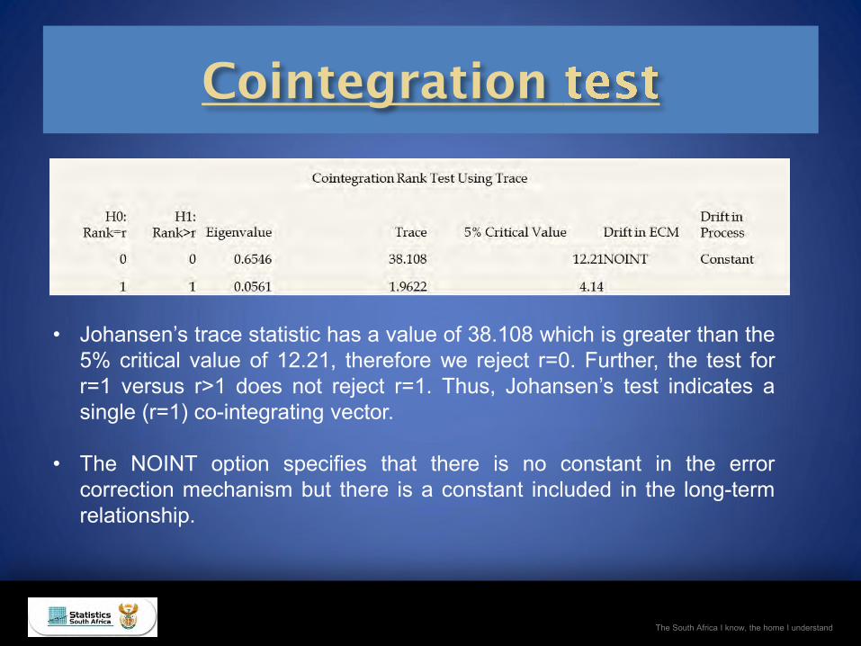
• Johansen’s trace statistic has a value of 38.108 which is greater than the 5% critical value of 12.21, therefore we reject r=0. Further, the test for r=1 versus r>1 does not reject r=1. Thus, Johansen’s test indicates a single (r=1) co-integrating vector.
• The NOINT option specifies that there is no constant in the error correction mechanism but there is a constant included in the long-term relationship.

The South Africa I know, the home I understand
Φ ∆x + ϵ t−1 t−i
∆x = Πx + Long term relationship in t ∑ p−1 ∗
i=1 i t
There is an adjustment to the ’equilibrium’ x ∗ or long term relation described by the
cointegrating relation.
› Setting ∆x = 0 we obtain the long run relation, i.e.
Πx ∗ = 0 This may be wirtten as
Πx ∗ = α(β′x ∗) = 0
In the case 0 < Rank(Π) = Rank(α) = m < k the number of solutions of this system of linear
equations which are different from zero is m.
β′x ∗ = 0m×1

The South Africa I know, the home I understand
30 / 58
Long term relationship
• The long run relation does not hold perfectly in (t − 1). There will be some deviation,
an error,
• β′xt−1 = ξt−1 ̸= 0
• The adjustment coefficients in α multiplied by the ’errors’ β′xt−1 induce adjustment.
They determine ∆xt , so that the x ’s move in the correct direction in order to bring the
system back to ’equilibrium’.
The South Africa I know, the home I understand

The South Africa I know, the home I understand
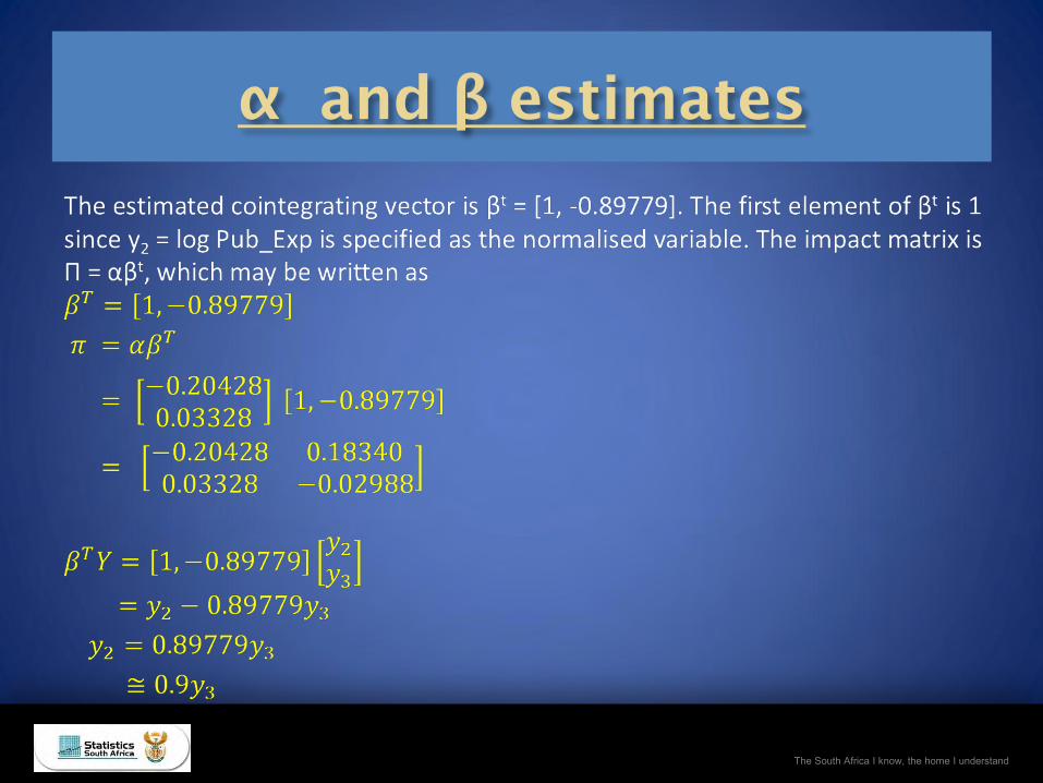
• βt Xt-1 measures error term: the deviation from the stationary mean at time t-1
• αβt Xt-1 = Π yt-1 ≡ Rate at which the series “ correct “from disequilibrium is represented by the adjustment vector α
• Π = αβt ≡ impact matrix (remember not unique)

The South Africa I know, the home I understand
• The residuals are checked for normality and autoregressive conditional heteroscedasticity or ARCH effects.
• The model also tests whether the residuals are correlated. The Durbin-Watson test statistics are both near 2 for both residual series suggesting no first order autocorrelation.
• The residuals do not deviate from normal (The residuals represent a white noise process).
• There are no ARCH effects on the residuals since the “no ARCH” hypothesis cannot be rejected given the F values (The residuals have equal covariances)

The South Africa I know, the home I understand
There are no AR effects on the residuals - for both residual series the autoregressive model fit to the residuals show no significance indicating that the residuals are uncorrelated

The South Africa I know, the home I understand

The South Africa I know, the home I understand


