

INTERLINKAGES AMONG SOUTH EAST ASIAN STOCK MARKETS
(A Comparison Between Pre- and Post-1997-Crisis Periods)
Research Paper ECO 2401S (Ph.D. Econometrics)
By Aamir R. Hashmi
Department of Economics University of Toronto
Student #: 992183882 Email: [email protected]

INTERLINKAGES AMONG SOUTH EAST ASIAN STOCK MARKETS (A Comparison Between Pre- and Post-1997-Crisis Periods)
Inter-linkages among New York (NY), Tokyo (TK) and five South East Asian (SEA) stock market returns (before and after the Asian currency crisis) are examined using tests on correlations and VAR models. Inter-linkages among SEA markets have increased after the emergence of crisis. More specifically the small markets have greater effect on large markets in the post-crisis period. NY affects SEA markets in both periods but is not affected by them. Effects of TK are low but have slightly increased after the crisis. Singapore stock market appears to be the leader in the region and its share in explaining variance of forecast error for regional markets is even greater than that of NY.
Key words: Stock Market Integration; South-East Asian Stock Markets
JEL classification: F15; G15
Studies of market integration suggest that international stock markets have become more
integrated in recent years.1 Although this evidence is not undisputed,2 most of the recent
studies find equity markets to be inter-linked. These linkages are attributable to the
deregulation of international financial markets, shift to floating exchange rates,
advancements in communication and information technology, lower costs of transactions
and the development of new financial instruments.
Some General Results from Earlier Studies
Studies have shown that New York stock market is the global leader and markets in
almost every region of the world are affected by it.3 It has also been documented that
markets tend to have stronger relations with geographically closer markets than with the
remote ones i.e. intra-regional linkages are stronger than inter-regional linkages.4
1 The studies that provide evidence that markets are integrated and/or their degree of integration has been changing (mostly increasing) over time include, among many others, Ammer and May (1996), Arshanapalli and Doukas (1993), Bracker et al (1999), Eun and Shim (1989), Kasa (1992), Leachman and Fransic (1995), Longin and Solnik (1995), Rangvid (2001) and Taylor and Tonks (1989). For a comprehensive bibliography of studies on international stock market linkages see Roca (2000) pp.148-171. 2 See King (1994) and Baekaert and Harvey (1995). 3 See, for example, Cheung and Mak (1992), Eun and Shim (1989), Koch and Koch (1993), Pesonen (1999) and Soydemir (2000). 4 See, for example, Hilliard (1979) and Dekker et al (2001).
2

Another finding is that linkages are variable over time and generally major events (like
1973 and 1979 oil price shocks, end of the Bretton Woods system, abolition of exchange
controls in UK in late 1970s, 1987 stock market crash, 1991 Gulf war etc.) affect the
linkages significantly.5
Why this Study?
The last conclusion is the motivation to study the effects of 1997 financial crisis on inter-
linkages among five major South East Asian (SEA) stock markets. There are studies that
concentrate on linkages among Asian markets6 but none has attempted to study the
effects of 1997 crisis on linkages. A recent paper by Jang and Sul (2002) studies the
effects of Asian financial crisis on co-movements of Asian stock markets. Besides
differences in coverage and methodology, their study does not include New York (NY)
stock market. We show below that NY market has a very strong effect on all the markets
in the region and any study of stock market linkages without NY may not capture the true
dynamics of linkages among these markets.
The basic questions that we try to answer in this study are: what is the nature of
linkages among SEA markets? Has the 1997 financial crisis changed these linkages? How
much of the movements in one stock market can be explained by innovations in other
markets? The basic hypothesis of this study is that in general the crisis should increase
intra-regional linkages. This hypothesis is in line with generally held view that during the
periods of uncertainly the correlations among the markets tend to increase.
5 See, for example, Ammer and Mei (1996), Arshanapalli and Doukas (1993), Leachman and Fransic (1995) and Taylor and Tonks (1989). 6 Examples include Pan et al (1999), Dekker et al (2001) and Siklos and Ng (2001).
3
Scope of the Study
Seven stock markets included in the study are: New York (NY), Tokyo (TK), Singapore
(SG), Kuala Lumpur (KL), Bangkok (BK), Jakarta (JK), and Manila (MN).7 The last five
constitute almost the entire South East Asia. Motivation for concentrating on the five SEA
markets is manifold. The Asian financial crisis began in Thailand and SEA markets were
among the worst victims of the crisis. It is interesting to see how this major event in the
economic history of Asia has affected the inter-linkages among these markets. Second,
these five economies have close economic and cultural links and both before and after the
crisis, the growth rates in these economies were strikingly correlated.8 Third, these
markets are geographically close to one another. There is some evidence in the literature,
as cited above, that geographically close markets tend to be more integrated with one
another.
The reason for including NY and TK in our sample is the following. Besides being the
two largest markets in the world, the US and Japan have very strong trade relations with
all five SEA markets in our sample. More specifically, more than one-third of all the
exports of these SEA markets go to either US or Japan. Similarly, more than a third of
their imports originate from one of the two countries.9 Another reason for including NY is
the general conclusion in the literature that NY stock market affects markets in almost all
regions of the world.
7 From this point onwards these acronyms are used instead of market names. 8 Average value of correlation coefficient between real GDP growth rates (from 1988 to 2001) for the five SEA economies in our sample is 0.65. 9 The last two statements are based on data provided by Economist Intelligence Unit. These data are available under the heading of ‘Fact Sheet’ for each country from http://www.economist.com/countries.
4

Data
The basic data are daily stock market closing indexes in terms of local currencies. The
indexes used are S&P 500 Composite, Nikkei 225 Stock Average, Singapore Straits
Times Index, Kuala Lumpur Composite, Bangkok SET, Jakarta SE Composite and
Philippines SE Composite. These data were downloaded from DataStream’s online
database. Data are reported on five-days-a-week basis and cover a time period from 1
January 1990 to 31 December 2002, which is divided into two sub-periods. The pre-crisis
period covers from 1 January 1990 to 31 July 1997 and the post-crisis period from 1
August 1997 to 31 December 2002. We assume that the value of an index remains
unchanged for the days when the market is closed.
The indexes are transformed into continuously compounded daily returns, defined as:
( ) 100lnln 1 ×−= −i
ti
tit PPR , where is stock price index series of market i. All markets
in the sample (except NY) operate in similar time zones and there is a lot of overlapping
in their trading hours. Since the study uses daily returns, all markets (except NY) are
treated as operating synchronously. NY is in a different time zone and opens when all
these markets have closed. For this reason correlations are computed using lagged returns
for NY and current returns for other markets.
itP
Methodology
Correlation matrices for various sub-periods are computed and their equality is tested
using Wald-like tests proposed by Goetzmann et al (2001) [from here on, GLR (2001)].
They use the asymptotic distribution of correlation matrix developed by Neudecker and
5

Wesselman (1990) and suggest two tests. The first test (from here on, ‘GLR Test 1’) is an
element-by-element test. The null and alternative hypotheses are:
PPPH == 210 : and Ω=Ω=Ω 21
211 : PPH ≠ or 21 Ω≠Ω
Under the null, the difference between two sample correlation matrices has the
following asymptotic distribution:
Ω
+
− →
∧∧
2121
11,0nn
NPPvecd
Where is the sample correlation matrix, niP∧
i is the number of observations for sub-
period i and is as defined in GLR et al (2001). Using this distribution they propose the
following test statistic:
Ω
( )( )Ω
−
Ω
+
− →
∧∧−
∧∧
RankPPvecnn
PPvecdT
221
1
2121
11 χ
The second (from here on, ‘GLR Test 2’) is to test the changes in average correlation.
Here the hypotheses are:
PPPH == 210 : and Ω=Ω= 21Ω
211 : PPH ≠ or Ω 21 Ω≠
The test statitic is:
( )111 221
1
2121 χ→
−
′Ω
+
−
∧∧−
∧∧ dT
PPvecki
ki
ki
nnPPvec
ki
Where k is the number of elements in ( )Pvec and is a i k×1 vector of ones.
6

Standard VAR models are estimated to study linkage dynamics for both pre- and post-
crisis periods. Many studies of stock markets have used VAR models to study inter-
linkages.10 Results of VAR models are then used to test for multivariate Granger causality
and to compute impulse response functions and decomposed variance of forecast errors.
These are standard time-series tools and do not need any further elaboration. A standard
reference for all these tools is Hamilton (1994).
Preliminary Findings and Correlation Tests11
In order to have some idea about the properties of the data we compute basic statistics for
all seven series of returns for both pre- and post-crisis periods (See Table 1). Mean and
median are generally lower for post crisis period. Variance is higher after the crisis for all
seven markets. Noticeable are the post-crisis variance numbers (which are all greater than
4) for KL, BK and JK. Changes in kurtosis are mixed and in four of the seven markets it
has increased while for the remaining three it has decreased. Although the plots of returns
series (not shown) suggest stationarity, we formally test for unit roots and are able to
reject the null of unit roots in all seven series of returns for both periods.
To study the possible lead-lag relations between different pairs of these markets,
cross-correlograms for each of the 21 pairs of markets for both periods have been
examined (results are not reported). Most of the significant correlations are confined to
the first two lags12 and there is hardly any significant correlation beyond that. This basic
finding will be useful later to determine lag length for VAR models.
10 Few examples include Ammer and Mei (1996), Chaudhary (1994), Eun and Shim (1989), King et al (1994), Rapach (2001), Roca (1999), Soydemir (2000) and Yuce and Mugan (2000). 11 For all empirical work, codes are written in MATLAB. These are available from author upon request. 12 Up to 20 lags are studied.
7

Before reporting the findings on correlation matrices, a word of caution is in line:
correlations between market returns vary a lot over time. To have a better idea of this
variation, rolling average correlation between all pairs of markets in the sample are
computed using a rolling window of 260 observations. Figure 1 plots the results.
Correlation varies a lot over time with a minimum of 0.015 and a maximum of 0.337.
Rolling correlations for individual pairs are also studied (results not reported here) and
different patterns of change are found with the common feature of huge variations over
time. This point needs to be kept in mind while interpreting the following results.
Table 2 reports simple correlations for pre- and post-crisis periods. Returns are highly
correlated between most of the markets and average value of the correlation coefficient is
0.243 in the pre-crisis period and 0.294 in the post-crisis period.13 Among all 21
correlations only 6 have declined in the post crisis period and 5 of these 6 involve KL.
The most remarkable numbers are those for SG and KL. The correlation between the two
declines from 0.668 in pre-crisis period to 0.369 in post-crisis period.
Keeping in view the fact that correlations vary over time we divide pre-crisis period
into eight and post-crisis into five sub-periods. GLR Tests 1 and 2 are used to test for the
significance of changes in correlation coefficients. GLR Test 1 is very strict and in all
cases rejects the null at 1% level of significance (results are not reported). This result is
not surprising because it tests for the difference between correlation coefficients on
element-by-element basis and huge variations in correlation coefficients make the
13 We use the current period returns for all markets except the NY market for which we use the previous day returns. The idea is that NY is likely to influence the other markets but not to be affected by them. We also try the current returns from the NY but its correlation with the current returns from other markets is negligible.
8

rejection of the null, that all the elements of correlation matrix remain the same, very
likely. Table 3 reports the results for GLR Test 2. Since this test is applied to the average
of elements in correlation matrix, we find sub-periods over which this average does not
change much. Two important facts emerge from Table 3. First, the jump in average
correlation after the emergence of crisis is not unique: there have been other periods in
which the correlation increased significantly. Second, after the crisis the fluctuations in
correlation have been mild as compared to pre-crisis period.
The VAR Models
VAR models for both periods are estimated using different lag lengths and AIC, SBC and
LR statistics are computed. SBC suggests one lag for both periods while AIC supports two
lags for pre- and one for post-crisis period.14 Results of pair-wise cross-correlograms
suggest that the maximum number of lags exhibiting significant correlations is two. Eun
and Shim (1989) also find that price changes in one market are transmitted to the other
markets within a maximum of 48 hours. In the light of above, VAR models with two lags
are estimated for both periods. Standard F-tests for the equality of estimated VAR
coefficients reject the null of equality in all markets except TK.
Multivariate Granger Causality Tests
Multivariate Granger causality tests are conducted by testing the hypothesis that all
coefficients of lagged returns of market j are equal to zero in equation i, where
. A simple F-test is used. A significant F-statistic implies that lagged
returns in market j Granger cause returns in market i. Table 4 reports the results. NY
[ 7,,2,1, K∈ji ]
14 The results of LR tests are not conclusive and will support unreasonably large number of lags. For example, for post-crisis period the LR test suggests 30 lags.
9

affects15 all other markets in both pre- and post crisis periods and is affected only by TK
in both periods and by SG in pre-crisis period. TK affects NY and SG in both periods and
KL only in pre-crisis period. NY affects TK in both periods and KL in post crisis period
only.
Now we turn to the results for mutual causality among SEA markets. In case of SG
and KL, the former affects the latter in pre-crisis period but not in the post-crisis period.
The latter affects the former in post- but not in pre-crisis period. SG does not affect JK in
any period, nor is affected by it. SG affects BK and MN in both periods but is affected by
them only in post-crisis period. KL affects BK and JK in pre- and SG and MN in post-
crisis period and is affected by SG in pre- and by JK in post-crisis period. Two general
conclusions emerge from Table 4. First, the linkages among SEA markets have slightly
increased after the crisis. Second, although the smaller markets do not affect larger
markets before the crisis, they do so after. It suggests that signals from small markets
were taken more seriously after the crisis than before.
Impulse Responses
Cholesky decomposition is used to compute impulse responses. An important question in
any such decomposition is that of ordering of markets starting from the most exogenous
one to the most endogenous one. The ordering is crucial and a major change in ordering
is bound to affect the results significantly. I use market capitalization as the criterion for
ordering starting from the highest. Although over the sample period ranking based on
market capitalization has not remained the same, the variations have been small. The
15 In this discussion we use the word affect to mean Granger cause. For example when we say NY affects TK, we mean that returns in NY Granger cause returns in TK.
10
following ordering is used in the discussion to follow: NY, TK, SG, KL, BK, JK, and MN.
We call this particular ordering NTSKBJM (using first letter of each market’s name). We
also use NTKSBJM ordering and shall comment on the results briefly in the next section.
Ordering is indeed a debatable question but our major assumption is that a bigger market
is more likely to affect a smaller market than to be affected by it. The closer this
assumption is to be true; the more acceptable is the ordering proposed above.
Figures 2 and 3 show plots of impulse response functions (for up to five days) for pre-
and post- crisis periods respectively. Response of a market to its own innovation is not
shown. Each figure can be thought of as a 6 5× matrix of sub-figures. For example,
Figure 2 (3,5) refers to sub-figure in third row and fifth column of Figure 2. This
subfigure plots the impulse response of MN to Cholesky one standard deviation
innovations in SG in pre-crisis period. In general the impulse responses are higher in post
crisis period. For example, compare subfigures (1,4), (2,4), (3,4), (5,2), (5,3), (5,4) and
(5,5) in Figures 1 and 2. Transmission of the shocks is complete in at most four periods in
almost all cases. Generally, we see higher responses to SG and BK in post-crisis period.
Variance Decomposition
Impulse responses show the effects for different days separately. If one is interested in
some kind of cumulative effect, the variance decomposition is a better tool. We focus on
SEA markets in what follows and compare the variance decomposition in two sub-
periods. All the following discussion is based on Tables 5 and 6 and in each case we
comment on decomposed variance on fifth day (when the transmission is almost
complete).
11
Starting with SG, we see that most of the forecast error variance is explained by
movements in its own returns and by the movements in the returns of NY and TK. More
specifically, in the pre-crisis period, NY and TK explain 12.5 and 5.6 percent of variation
in SG returns respectively. These numbers increase slightly for post-crisis period.
In case of KL, SG explains a major proportion of its variance before the crisis (34.0
percent) but after the crisis it falls to mere 7.7 percent. When this result is viewed
together with the Granger causality test results, it supports the claim that KL has been
alienated from the region after the crisis. One possible explanation is the way in which
Malaysian government responded to the crisis by imposing capital controls. NY and TK
explained 4.7 and 1.9 percent of the variation in KL returns before the crisis. This
increased to 7.6 and 3.6 percent, respectively. Two important points emerges here. First,
KL has aliened from the region and responds more to shocks from NY and TK after the
crisis. Second, although NY and TK precede SG in our ordering, SG explains more of the
variations in variance of KL returns than both NY and TK. This is a significant finding
and we see below that it is true for other three SEA markets as well.
For BK too, the share of SG in explaining the forecast error variance is higher than
any other foreign market. It was 10.3 percent before the crisis and 15.6 percent after. The
share of NY slightly decreased from 5.5 to 4.6 percent in the post-crisis period and that of
TK increased from 0.8 to 3.0 percent. The implication is that SG acts as a leader for BK
both before and after the crisis and its effect has grown stronger in the later period.
JK appears to have become more sensitive to all bigger markets (except KL) after the
crisis. Before the crisis 88.3 percent of the variation in its returns was due to its own
12

shocks. This is reduced to 78.4 percent after the crisis. Although influence of all markets
has increased, once again the influence of SG dominates that of others.
Story for MN is similar to that of JK. All the markets influence MN more after the
crisis. Once again we notice that SG has the strongest effect and its share in explaining
the variance has almost doubled in the post-crisis period.
Before drawing any general conclusions, a brief comment on variance decomposition
results using NTKSBJM ordering is appropriate.16 The conclusion about SG’s regional
leadership is sensitive to the ordering in the pre-crisis period. When we change the
ordering to NTKSBJM, KL appears to affect the regional markets more than SG in pre-
crisis period. However, in the post-crisis period SG emerges as a clear leader regardless
of the ordering.
Summing up, the crisis has made all SEA markets (except KL), more sensitive to
variations in regional markets. KL appears to have become less sensitive to regional
markets after the crisis and slightly more to NY and TK. SG acts as a regional leader and
its effect on the regional markets in terms of explaining the variance of the forecast errors
is even greater than that of NY. This leadership has become stronger after the crisis.
Conclusions
Inter-linkages among SEA market have generally increased after the emergence of Asian
financial crisis in 1997. Small markets tend to affect big markets more after the crisis.
This conclusion applies only to SEA markets and not to NY and TK. NY affects SEA
markets both before and after the crisis, though they do not affect it. TK has little
16 Note the difference from previous ordering; KL and SG have switched positions.
13
influence on these markets before the crisis but its effect has slightly increased after the
crisis.
SG emerges as a leader in the region and its leadership is stronger in the post-crisis
period. The basic proof of its leadership lies in the higher percentage of variance in the
regional markets that can be explained by a shock in SG. Based on this criterion, the
influence of SG on the region is even greater than that of NY.
KL appears to have been alienated from the region after the crisis. This alienation
could be the consequence of capital control policies of the Malaysian government. BK
affects the region more after the crisis. JK also has an increased effect while MN, being
the smallest of five SEA markets studied, does not have much influence on other markets.
14

REFERENCES
Ammer, J. and Mei J. (1996), “Measuring International Economic Linkages with Stock
Market Data,” J of Finance, 5, 1743-63.
Arshanapalli, B. and Doukas, J. (1993), “International Stock Market Linkages: evidence
from the pre- and post-October 1987 period,” J of Banking and Finance, 17, 193-208.
Bekaert, G. and Harvey, C. R. (1995), “Time-Varying World Market Integration,” J of
Finance, 50, 403-44.
Bracker, K., Docking, D.S. and Koch, P.D. (1999), “Economic Determinants of
Evolution in International Stock Market Integration,” J of Empirical Finance, 6, 1-27.
Cheung, Y. L. and Mak, S. C. (1992), “The International Transmission of Stock Market
Fluctuations between the Developed Markets and the Asia-Pacific Markets,” Applied
Financial Economics, 2, 43-47.
Chowdhury, A. R. (1994), “Stock Market Independencies: Evidence form the Asian
NIE’s,” J of Macroeconomics, 16, 629-51.
Dekker, A., Sen, K. and Young, M. R. (2001), “Equity Market Linkages in the Asia
Pacific region: A Comparison of the Orthogonalised and Generalised VAR
Approaches,” Global Finance Journal, 12, 1-33.
Eun, C. S. and Shim, S. (1989), “ International Transmission of Stock Market
Movements,” J of Financial and Quantitative Analysis, 24, 241-56.
Goetzmann, W. N., Li, L. and Rouwenhorst, K. G. (2001), “Long-term Global Market
Correlations,” NBER Working Paper 8612, November.
Hamilton, J. D. (1994), “Time Series Analysis,” Princeton Univ Press, Princeton, NJ.
Hilliard, J.E. (1979), “The Relationship Between Equity Indices on World Exchanges,” J
of Finance, 34, 103-14.
Kasa, K. (1992), “Common Stochastic Trends in International Stock Markets,” J of
Monetary Economics, 29, 95-124.
King, M. A., Sentana, E. and Wadhwani, S. B. (1994), “Volatility and Links between
National Stock Markets,” Econometrica, 62, 901-33.
Koch, T.W. and Koch, P.D. (1993), “Dynamic Relationship among the Daily Level of
National Stock Indexes” in International Financial Market Integration. Stansell, S. R.
(ed.), Blackwells, Mass.
15
Leachman, L. L. and Fransic, B. (1995), “ Long-run Relations Among the G-5 and G-7
Equity Markets: Evidence on the Plaza and Louvre Accords,” J of Macroeconomics,
17, 551-77.
Longin, F. and Solnik B. (1995), “Is the Correlation in International Equity Returns
Constant: 1960-1990?” J of International Money and Finance, 14, 3-26.
Neudecker, H. and Wesselman, A. M. (1990), “The Asymptotic Variance Matrix of the
Sample Correlation Matrix,” Linear Algebra and its Applications, 127, 589-99.
Pan, M. S., Liu, Y. A. and Roth, H. J. (1999), “Common Stochastic Trends and Volatility
in Asian-Pacific Equity Markets,” Global Finance Journal, 10, 161-72.
Pesonen, H. (1999), “Assessing Causal Linkages Between the Emerging Stock Markets
of Asia and Russia,” Russian and East European Finance and Trade, 35, 73-82.
Rangvid, J. (2001), “Increasing Convergence Among European Stock Markets? A
Recursive Common Stochastic Trends Analysis,” Economics Letters, 71, 383-89.
Rapach, D. E. (2001), “Macro Shocks and Real Stock Prices,” J of Economics and
Business, 53, 5-26.
Roca, E. D. (1999), “Short-term and Long-term Price Linkages Between the Equity
Markets of Australia and its Major Trading Partners,” Applied Financial Economics,
9, 501-11.
Roca, E. D. (2000), “Price Interdependence Among Equity Markets in the Asia-Pacific
Region: Focus on Australia and ASEAN,” Ashgate, England.
Siklos, P. L. and Patrick, N. (2001), “Integration Among Asia-Pacific and International
Stock Markets: Common Stochastic Trends and Regime Shifts,” Pacific Economic
Review, 6, 89-110.
Soydemir, G. (2000), “International Transmission Mechanism of Stock Market
Movements: Evidence from Emerging Equity Markets,” J of Forecasting, 19, 149-76.
Taylor, M. P. and Tonks, I. (1989), “The Internationalization of Stock Markets and the
Abolition of UK exchange Controls,” Review of Economics and Statistics, 71, 332-36.
Yuce, A. and Mugan, C. S. (2000), “Linkages Among Eastern European Stock Markets
and the Major Stock Exchanges,” Russian and East European Finance and Trade, 36,
54-69.
16
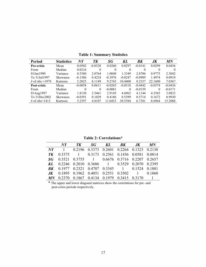
Table 1: Summary Statistics
Period Statistics NY TK SG KL BK JK MN Mean 0.0502 -0.0328 0.0260 0.0297 -0.0141 0.0299 0.0436 Median 0.0216 0 0 0 0 0 0 Variance 0.5380 2.0764 1.0048 1.3349 2.8706 0.9775 2.3042 Skewness -0.1586 0.4224 -0.3976 -0.0247 -0.0989 1.4974 0.0919
Pre-crisis From 01Jan1990 To 31Jul1997 # of obs =1979 Kurtosis 5.2025 8.1149 9.2743 10.4400 8.2337 22.1600 7.0367
Mean -0.0058 0.0611 -0.0265 -0.0318 -0.0442 -0.0374 -0.0436 Median 0 0 -0.0081 0 -0.0159 0 -0.0171 Variance 1.8120 2.5461 2.9145 4.6962 4.1144 4.3565 3.0832 Skewness -0.0391 0.1029 0.4186 0.5399 0.5714 0.1672 0.9930
Post-crisis From 01Aug1997 To 31Dec2002 # of obs=1413 Kurtosis 5.2397 4.8107 11.0453 30.5384 6.7381 8.6964 15.2088
Table 2: Correlations*
NY TK SG KL BK JK MN NY 1 0.2196 0.3373 0.2601 0.2264 0.1323 0.2130 TK 0.3375 1 0.3173 0.2561 0.1436 0.0581 0.0814 SG 0.3521 0.3755 1 0.6676 0.3716 0.2207 0.2657 KL 0.2246 0.2010 0.3686 1 0.3529 0.2070 0.2395 BK 0.1977 0.2321 0.4707 0.3345 1 0.1524 0.1881 JK 0.1895 0.1962 0.4051 0.2551 0.3502 1 0.1860 MN 0.2370 0.1867 0.4134 0.1979 0.3415 0.3170 1 * The upper and lower diagonal matrices show the correlations for pre- and
post-crisis periods respectively.
17
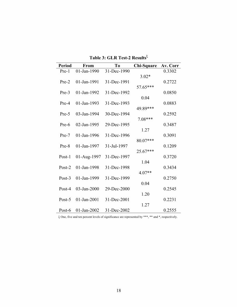
Table 3: GLR Test-2 Resultsξ
Period From To Chi-Square Av. Corr Pre-1 01-Jan-1990 31-Dec-1990 0.3302
3.02* Pre-2 01-Jan-1991 31-Dec-1991 0.2722
57.65*** Pre-3 01-Jan-1992 31-Dec-1992 0.0850
0.04 Pre-4 01-Jan-1993 31-Dec-1993 0.0883
49.89*** Pre-5 03-Jan-1994 30-Dec-1994 0.2592
7.08*** Pre-6 02-Jan-1995 29-Dec-1995 0.3487
1.27 Pre-7 01-Jan-1996 31-Dec-1996 0.3091
80.07*** Pre-8 01-Jan-1997 31-Jul-1997 0.1209
25.67*** Post-1 01-Aug-1997 31-Dec-1997 0.3720
1.04 Post-2 01-Jan-1998 31-Dec-1998 0.3434
4.07** Post-3 01-Jan-1999 31-Dec-1999 0.2750
0.04 Post-4 03-Jan-2000 29-Dec-2000 0.2545
1.20 Post-5 01-Jan-2001 31-Dec-2001 0.2231
1.27 Post-6 01-Jan-2002 31-Dec-2002 0.2555 ξ One, five and ten percent levels of significance are represented by ***, ** and *, respectively.
18

Table 4: Multivariate Granger Causality Test Resultsξ
F-Statistic F-Statistic Pre-crisis Post-crisis Pre-crisis Post-crisis
NY→TK 48.3168*** 94.8184*** TK→NY 2.4551* 2.3152*
NY→SG 112.7772*** 96.2509*** SG→NY 5.0867*** 1.9307
NY→KL 59.2520*** 34.8873*** KL→NY 1.2135 2.2109
NY→BK 40.9070*** 25.2207*** BK→NY 1.2367 2.4848*
NY→JK 17.2189*** 27.1965*** JK→NY 1.3252 0.6192
NY→MN 41.2516*** 38.1535*** MN→NY 0.8489 0.1111
TK→SG 2.6209* 3.7417** SG→TK 1.9540 0.0782
TK→KL 3.5069** 0.5140 KL→TK 0.0917 2.6727*
TK→BK 0.9357 1.7587 BK→TK 1.6538 0.6170
TK→JK 2.1618 2.3896* JK→TK 0.4510 0.1485
TK→MN 2.2532 1.7945 MN→TK 2.1627 0.1326
SG→KL 12.1849*** 1.2979 KL→SG 0.9905 2.5383*
SG→BK 11.7358*** 3.7250** BK→SG 1.2615 3.9109**
SG→JK 1.4025 1.2675 JK→SG 0.7730 1.3807
SG→MN 8.6820*** 4.5682** MN→SG 0.7067 3.7188**
KL→BK 3.1688** 0.0281 BK→KL 0.1610 1.0856
KL→JK 5.4977*** 0.3139 JK→KL 0.6372 10.9226***
KL→MN 1.2829 4.3603** MN→KL 0.5869 1.1422
BK→JK 3.2748** 7.4177*** JK→BK 2.3138* 3.8551**
BK→MN 3.0776** 8.5430*** MN→BK 1.4324 1.1996
JK→MN 1.5408 3.4222** MN→JK 5.0710*** 2.0180
ξ One, five and ten percent levels of significance are represented by ***, ** and *, respectively.
19

Table 5: Variance Decomposition with NTSKBJM Ordering (Pre-Crisis)
Period NY TK SG KL BK JK MN Variance Decomposition of NY:
1 100.0000 0 0 0 0 0 02 99.3093 0.0767 0.4124 0.0815 0.0455 0.0131 0.06165 98.7193 0.2439 0.5331 0.1829 0.1154 0.1250 0.0804
Variance Decomposition of TK: 1 1.2787 98.7213 0 0 0 0 02 5.7530 93.9566 0.0848 0.0156 0.1457 0.0034 0.04105 5.8364 93.4668 0.1932 0.0237 0.1831 0.0467 0.2501
Variance Decomposition of SG: 1 1.3982 6.5901 92.0117 0 0 0 02 12.3340 5.6471 81.7920 0.0182 0.0890 0.0692 0.05045 12.5055 5.6277 81.4381 0.1693 0.1013 0.1001 0.0580
Variance Decomposition of KL: 1 1.1046 4.0367 34.4039 60.4548 0 0 02 7.3872 3.6427 33.9194 54.9486 0.0068 0.0633 0.03195 7.6256 3.6153 33.9690 54.6561 0.0122 0.0826 0.0392
Variance Decomposition of BK: 1 0.3564 0.8626 7.5964 1.5071 89.6775 0 02 5.1328 0.8388 10.1206 1.6756 82.0602 0.1705 0.00165 5.4594 0.8494 10.3325 1.7605 81.3265 0.1995 0.0721
Variance Decomposition of JK: 1 0.0005 0.1088 3.3180 0.3757 0.1499 96.0472 02 1.7043 0.1277 5.2495 1.2095 0.5562 90.9330 0.21985 1.8693 0.1622 7.1105 1.3622 0.6198 88.3053 0.5706
Variance Decomposition of MN: 1 0.2085 0.1187 3.3687 0.4319 0.2178 0.4915 95.16292 4.5187 0.8125 6.3333 0.6327 0.5333 0.5237 86.64585 4.5412 0.8795 6.7857 0.6715 0.5326 0.6085 85.9809
20
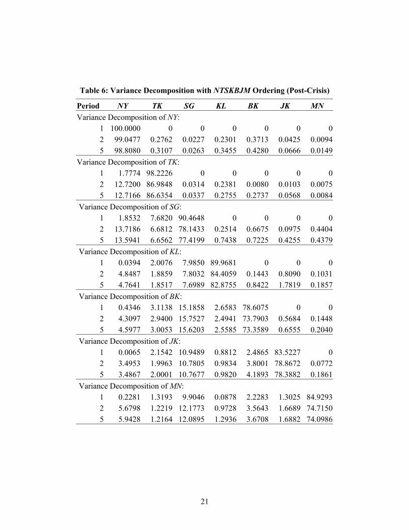
Table 6: Variance Decomposition with NTSKBJM Ordering (Post-Crisis)
Period NY TK SG KL BK JK MN Variance Decomposition of NY:
1 100.0000 0 0 0 0 0 02 99.0477 0.2762 0.0227 0.2301 0.3713 0.0425 0.00945 98.8080 0.3107 0.0263 0.3455 0.4280 0.0666 0.0149
Variance Decomposition of TK: 1 1.7774 98.2226 0 0 0 0 02 12.7200 86.9848 0.0314 0.2381 0.0080 0.0103 0.00755 12.7166 86.6354 0.0337 0.2755 0.2737 0.0568 0.0084
Variance Decomposition of SG: 1 1.8532 7.6820 90.4648 0 0 0 02 13.7186 6.6812 78.1433 0.2514 0.6675 0.0975 0.44045 13.5941 6.6562 77.4199 0.7438 0.7225 0.4255 0.4379
Variance Decomposition of KL: 1 0.0394 2.0076 7.9850 89.9681 0 0 02 4.8487 1.8859 7.8032 84.4059 0.1443 0.8090 0.10315 4.7641 1.8517 7.6989 82.8755 0.8422 1.7819 0.1857
Variance Decomposition of BK: 1 0.4346 3.1138 15.1858 2.6583 78.6075 0 02 4.3097 2.9400 15.7527 2.4941 73.7903 0.5684 0.14485 4.5977 3.0053 15.6203 2.5585 73.3589 0.6555 0.2040
Variance Decomposition of JK: 1 0.0065 2.1542 10.9489 0.8812 2.4865 83.5227 02 3.4953 1.9963 10.7805 0.9834 3.8001 78.8672 0.07725 3.4867 2.0001 10.7677 0.9820 4.1893 78.3882 0.1861
Variance Decomposition of MN: 1 0.2281 1.3193 9.9046 0.0878 2.2283 1.3025 84.92932 5.6798 1.2219 12.1773 0.9728 3.5643 1.6689 74.71505 5.9428 1.2164 12.0895 1.2936 3.6708 1.6882 74.0986
21
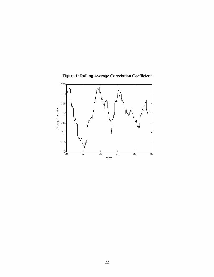
Figure 1: Rolling Average Correlation Coefficient
22

Figure 2: Impulse Response Functions (Pre-crisis Period)
• ‘Res of x to y’ means impulse response of market ‘x’ to Cholesky one standard deviation innovation in market ‘y’. • The numbers on x-axis are number of days.
23
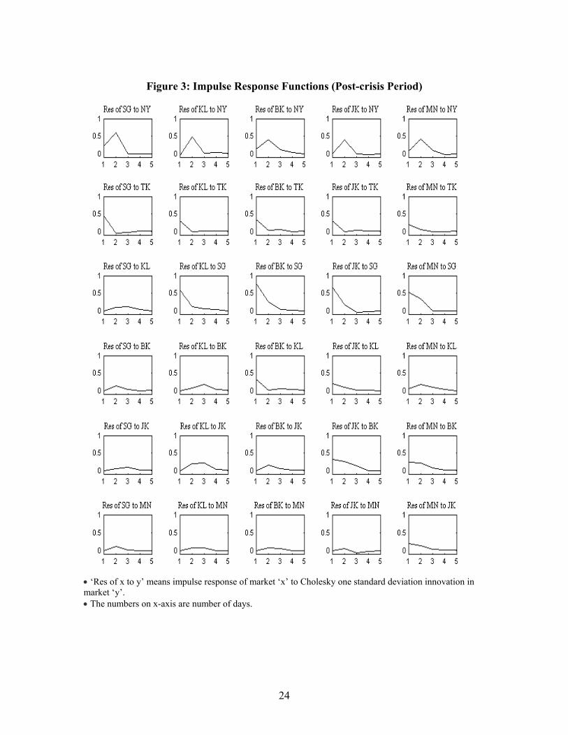
Figure 3: Impulse Response Functions (Post-crisis Period)
• ‘Res of x to y’ means impulse response of market ‘x’ to Cholesky one standard deviation innovation in market ‘y’. • The numbers on x-axis are number of days.
24


