

UCLA Department of StatisticsStatistical Consulting Center
Intro to Spatial Statistics in R
David Diez
June 2, 2009
David Diez
Intro to Spatial Statistics in R UCLA Department of Statistics Statistical Consulting Center
Prerequisites
It is assumed that an attendant has...
A strong understanding of basic probability theory.
Taken a regression course.
Familiarity with using R for regression and building very simplefunctions.
David Diez
Intro to Spatial Statistics in R UCLA Department of Statistics Statistical Consulting Center
Outline
Geostatistics
Regression modelingKrigingCorrelogram (in passing)
Point patterns
Poisson theoryClusteringTools to ID clusteringInhibition
David Diez
Intro to Spatial Statistics in R UCLA Department of Statistics Statistical Consulting Center
Introduction Modeling Kriging Correlogram
Geostats
Geostats
Geostatistical data includes observationsat a collection of locations. Thelocations may or may not be random,and it is what is observed at theselocations that is of particular interest.
Later we will discuss point pattern data,where the points themselves are thedata (such as earthquake locations).
David Diez
Intro to Spatial Statistics in R UCLA Department of Statistics Statistical Consulting Center
Introduction Modeling Kriging Correlogram
Packages
Packages
We will need the spatial and MASS packages:
> library(spatial)> library(MASS)
spatial is included in the initial R install, however, MASS is not. Ifloading MASS does not work, first install the package:
> install.packages("MASS")
David Diez
Intro to Spatial Statistics in R UCLA Department of Statistics Statistical Consulting Center
Introduction Modeling Kriging Correlogram
topo
Data
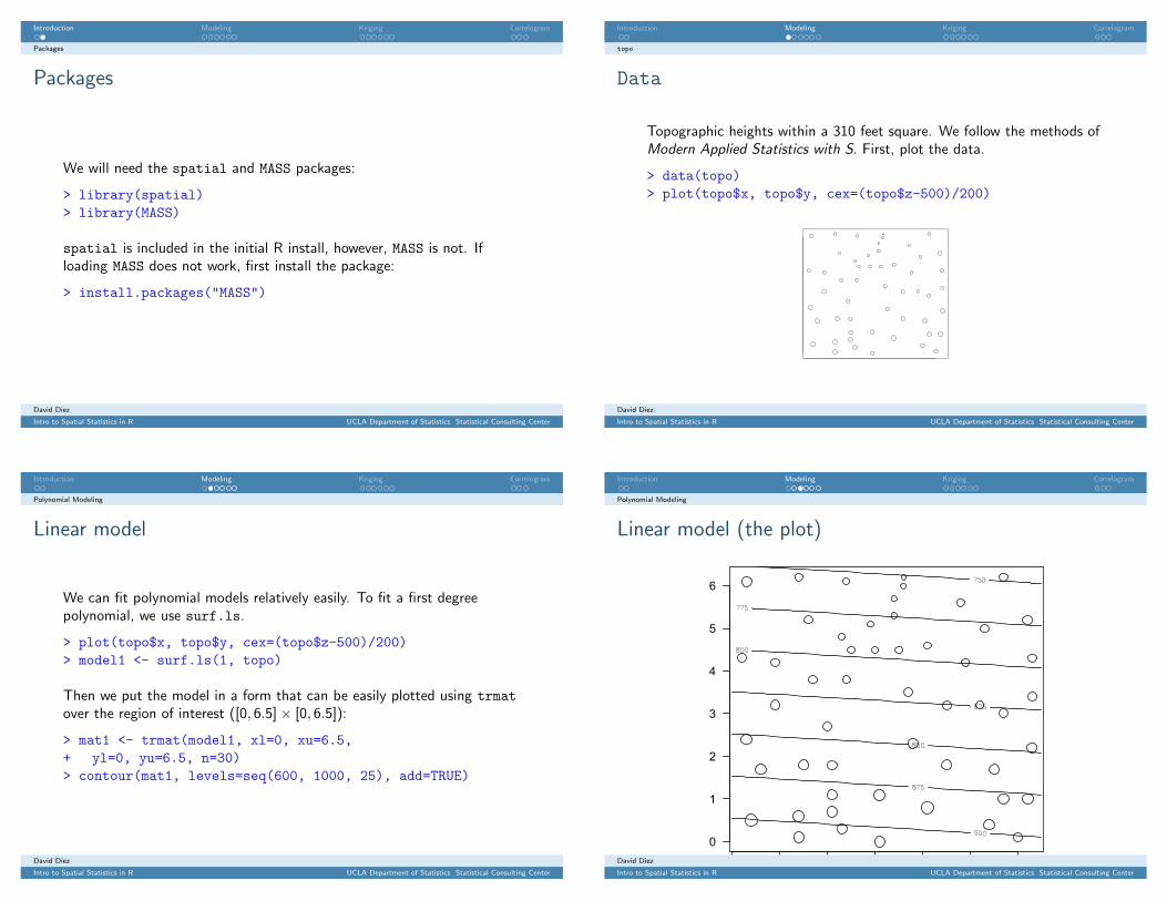
Topographic heights within a 310 feet square. We follow the methods ofModern Applied Statistics with S. First, plot the data.
> data(topo)> plot(topo$x, topo$y, cex=(topo$z-500)/200)
David Diez
Intro to Spatial Statistics in R UCLA Department of Statistics Statistical Consulting Center
Introduction Modeling Kriging Correlogram
Polynomial Modeling
Linear model
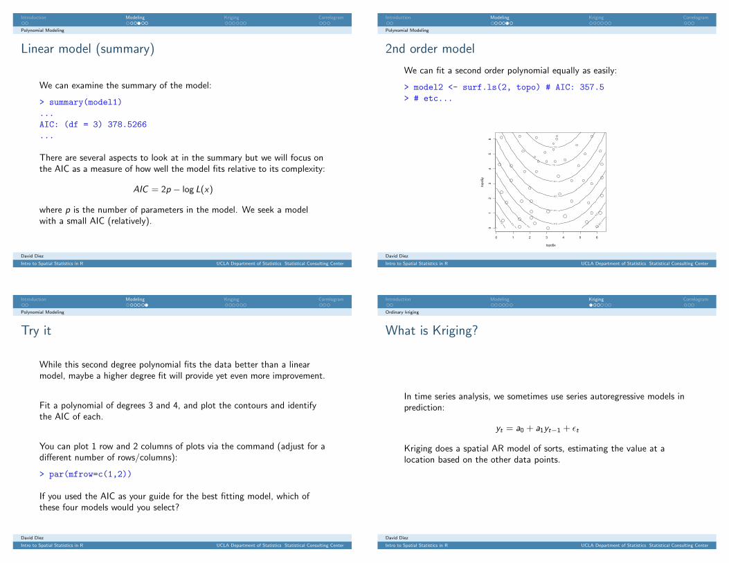
We can fit polynomial models relatively easily. To fit a first degreepolynomial, we use surf.ls.
> plot(topo$x, topo$y, cex=(topo$z-500)/200)> model1 <- surf.ls(1, topo)
Then we put the model in a form that can be easily plotted using trmatover the region of interest ([0, 6.5]× [0, 6.5]):
> mat1 <- trmat(model1, xl=0, xu=6.5,+ yl=0, yu=6.5, n=30)> contour(mat1, levels=seq(600, 1000, 25), add=TRUE)
David Diez
Intro to Spatial Statistics in R UCLA Department of Statistics Statistical Consulting Center
Introduction Modeling Kriging Correlogram
Polynomial Modeling
Linear model (the plot)
0 1 2 3 4 5 6
0
1
2
3
4
5
6
David Diez
Intro to Spatial Statistics in R UCLA Department of Statistics Statistical Consulting Center
Introduction Modeling Kriging Correlogram
Polynomial Modeling
Linear model (summary)
We can examine the summary of the model:
> summary(model1)...AIC: (df = 3) 378.5266...
There are several aspects to look at in the summary but we will focus onthe AIC as a measure of how well the model fits relative to its complexity:
AIC = 2p − log L(x)
where p is the number of parameters in the model. We seek a modelwith a small AIC (relatively).
David Diez
Intro to Spatial Statistics in R UCLA Department of Statistics Statistical Consulting Center
Introduction Modeling Kriging Correlogram
Polynomial Modeling
2nd order model
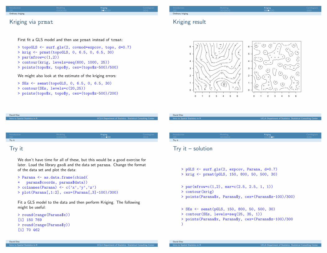
We can fit a second order polynomial equally as easily:
> model2 <- surf.ls(2, topo) # AIC: 357.5> # etc...
0 1 2 3 4 5 6
01
23
45
6
topo$x
topo$y
David Diez
Intro to Spatial Statistics in R UCLA Department of Statistics Statistical Consulting Center
Introduction Modeling Kriging Correlogram
Polynomial Modeling
Try it
While this second degree polynomial fits the data better than a linearmodel, maybe a higher degree fit will provide yet even more improvement.
Fit a polynomial of degrees 3 and 4, and plot the contours and identifythe AIC of each.
You can plot 1 row and 2 columns of plots via the command (adjust for adifferent number of rows/columns):
> par(mfrow=c(1,2))
If you used the AIC as your guide for the best fitting model, which ofthese four models would you select?
David Diez
Intro to Spatial Statistics in R UCLA Department of Statistics Statistical Consulting Center
Introduction Modeling Kriging Correlogram
Ordinary kriging
What is Kriging?
In time series analysis, we sometimes use series autoregressive models inprediction:
yt = a0 + a1yt−1 + εt
Kriging does a spatial AR model of sorts, estimating the value at alocation based on the other data points.
David Diez
Intro to Spatial Statistics in R UCLA Department of Statistics Statistical Consulting Center
Introduction Modeling Kriging Correlogram
Ordinary kriging
Kriging via prmat
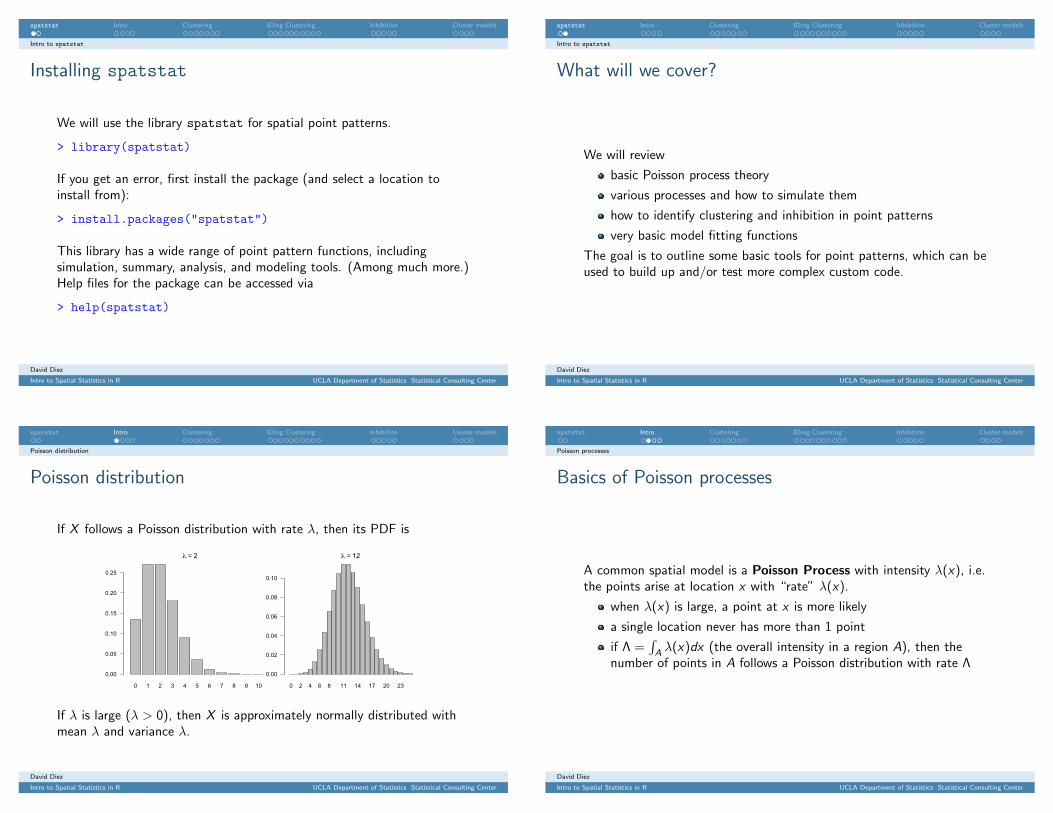
First fit a GLS model and then use prmat instead of trmat:
> topoGLS <- surf.gls(2, covmod=expcov, topo, d=0.7)> krig <- prmat(topoGLS, 0, 6.5, 0, 6.5, 30)> par(mfrow=c(1,2))> contour(krig, levels=seq(600, 1000, 25))> points(topo$x, topo$y, cex=(topo$z-500)/500)
We might also look at the estimate of the kriging errors:
> SEs <- semat(topoGLS, 0, 6.5, 0, 6.5, 30)> contour(SEs, levels=c(20,25))> points(topo$x, topo$y, cex=(topo$z-500)/200)
David Diez
Intro to Spatial Statistics in R UCLA Department of Statistics Statistical Consulting Center
Introduction Modeling Kriging Correlogram
Ordinary kriging
Kriging result
0 1 2 3 4 5 6
0
1
2
3
4
5
6
0 1 2 3 4 5 6
0
1
2
3
4
5
6
David Diez
Intro to Spatial Statistics in R UCLA Department of Statistics Statistical Consulting Center
Introduction Modeling Kriging Correlogram
Try it
Try it
We don’t have time for all of these, but this would be a good exercise forlater. Load the library geoR and the data set parana. Change the formatof the data set and plot the data:
> Parana <- as.data.frame(cbind(+ parana$coords, parana$data))> colnames(Parana) <- c(’x’,’y’,’z’)> plot(Parana[,1:2], cex=(Parana[,3]-100)/300)
Fit a GLS model to the data and then perform Kriging. The followingmight be useful:
> round(range(Parana$x))[1] 150 769> round(range(Parana$y))[1] 70 462
David Diez
Intro to Spatial Statistics in R UCLA Department of Statistics Statistical Consulting Center
Introduction Modeling Kriging Correlogram
Try it
Try it – solution
> pGLS <- surf.gls(2, expcov, Parana, d=0.7)> krig <- prmat(pGLS, 150, 800, 50, 500, 30)
> par(mfrow=c(1,2), mar=c(2.5, 2.5, 1, 1))> contour(krig)> points(Parana$x, Parana$y, cex=(Parana$z-100)/300)
> SEs <- semat(pGLS, 150, 800, 50, 500, 30)> contour(SEs, levels=seq(25, 35, 1))> points(Parana$x, Parana$y, cex=(Parana$z-100)/300)
David Diez
Intro to Spatial Statistics in R UCLA Department of Statistics Statistical Consulting Center

Introduction Modeling Kriging Correlogram
Try it
Try it – solution (cont)
200 300 400 500 600 700 800
100
200
300
400
500
200 300 400 500 600 700 800
100
200
300
400
500
David Diez
Intro to Spatial Statistics in R UCLA Department of Statistics Statistical Consulting Center
Introduction Modeling Kriging Correlogram
Theory
Theory
Used in kriging is the covariogram, a measure of the distance betweentwo observations:
C (x , y) = c(d(x , y))
Then c(r) is the covariation between observations a distance r apart.The correlogram is just the standardized covariogram.
David Diez
Intro to Spatial Statistics in R UCLA Department of Statistics Statistical Consulting Center
Introduction Modeling Kriging Correlogram
Theory
Covariogram models
The exponential and Gaussian covariance models assume the covariancefollows a parametric model:
c(r) = σ2e−r/d (exponential)
c(r) = σ2e−(r/d)2
(Gaussian)
where d is a parameter specified by the user (why specified?).
David Diez
Intro to Spatial Statistics in R UCLA Department of Statistics Statistical Consulting Center
Introduction Modeling Kriging Correlogram
Theory
topo correlogram of GLS residuals
> correlogram(topoGLS, 25)> r <- seq(0, 7, 0.1)> lines(r, expcov(r, d=0.7))> lines(r, gaucov(r,d=1,.3),+ lty=2)
> legend(’bottomleft’, lty=2,+ legend=c(’exponential’,+ ’gaussian’))
0 1 2 3 4 5 6 7
-1.0
-0.5
0.0
0.5
1.0
exponentialGaussian
David Diez
Intro to Spatial Statistics in R UCLA Department of Statistics Statistical Consulting Center
spatstat Intro Clustering IDing Clustering Inhibition Cluster models
Intro to spatstat
Installing spatstat
We will use the library spatstat for spatial point patterns.
> library(spatstat)
If you get an error, first install the package (and select a location toinstall from):
> install.packages("spatstat")
This library has a wide range of point pattern functions, includingsimulation, summary, analysis, and modeling tools. (Among much more.)Help files for the package can be accessed via
> help(spatstat)
David Diez
Intro to Spatial Statistics in R UCLA Department of Statistics Statistical Consulting Center
spatstat Intro Clustering IDing Clustering Inhibition Cluster models
Intro to spatstat
What will we cover?
We will review
basic Poisson process theory
various processes and how to simulate them
how to identify clustering and inhibition in point patterns
very basic model fitting functions
The goal is to outline some basic tools for point patterns, which can beused to build up and/or test more complex custom code.
David Diez
Intro to Spatial Statistics in R UCLA Department of Statistics Statistical Consulting Center
spatstat Intro Clustering IDing Clustering Inhibition Cluster models
Poisson distribution
Poisson distribution
If X follows a Poisson distribution with rate λ, then its PDF is
0 1 2 3 4 5 6 7 8 9 10
λ = 2
0.00
0.05
0.10
0.15
0.20
0.25
0 2 4 6 8 11 14 17 20 23
λ = 12
0.00
0.02
0.04
0.06
0.08
0.10
If λ is large (λ > 0), then X is approximately normally distributed withmean λ and variance λ.
David Diez
Intro to Spatial Statistics in R UCLA Department of Statistics Statistical Consulting Center
spatstat Intro Clustering IDing Clustering Inhibition Cluster models
Poisson processes
Basics of Poisson processes
A common spatial model is a Poisson Process with intensity λ(x), i.e.the points arise at location x with “rate” λ(x).
when λ(x) is large, a point at x is more likely
a single location never has more than 1 point
if Λ =∫Aλ(x)dx (the overall intensity in a region A), then the
number of points in A follows a Poisson distribution with rate Λ
David Diez
Intro to Spatial Statistics in R UCLA Department of Statistics Statistical Consulting Center

spatstat Intro Clustering IDing Clustering Inhibition Cluster models
Poisson processes
Example: Poisson process
To create a Poisson process with uniformintensity of 50 over [0, 1]× [0, 1],
> pp0 <- rpoispp(50)> plot(pp0)
To create the Poisson process with rate50 ∗ (x2 + y2) over [0, 1]× [0, 1],
> pp1 <- rpoispp(function(x,y)+ { 50*(x2̂+y2̂) })> plot(pp1)
pp0
pp1
David Diez
Intro to Spatial Statistics in R UCLA Department of Statistics Statistical Consulting Center
spatstat Intro Clustering IDing Clustering Inhibition Cluster models
Poisson processes
The ppp class
The package spatstat uses a special class for points called ppp. Thecoordinates of the points in a ppp object can be accessed via
> pp1$x[1] 0.965859088 0.9874...
> pp1$y[1] 0.787572894 0.0075...
Objects of class ppp also maintain other components, including the spaceover which points are observed, the number of points in the pattern, andany “marks” associated with the pattern (for instance, earthquakes mightbe marked by their magnitude).
David Diez
Intro to Spatial Statistics in R UCLA Department of Statistics Statistical Consulting Center
spatstat Intro Clustering IDing Clustering Inhibition Cluster models
Identifying clustering
Pop quiz
Do any of the following patterns show clustering?
David Diez
Intro to Spatial Statistics in R UCLA Department of Statistics Statistical Consulting Center
spatstat Intro Clustering IDing Clustering Inhibition Cluster models
Identifying clustering
Pop quiz: solution
None are clustered processes. The points are all uniformly distributedover the space (generated from a uniform intensity, i.e. homogeneous,Poisson process).
rpoispp(50) rpoispp(50) rpoispp(50)
David Diez
Intro to Spatial Statistics in R UCLA Department of Statistics Statistical Consulting Center

spatstat Intro Clustering IDing Clustering Inhibition Cluster models
Clustering processes
Neyman-Scott
A Neyman-Scott process is basically a Poisson process with each(“parent”) point (red) replaced with k uniformly distributed “children”points about it (black). Generate such a process via
> par(mar=rep(0, 4))> pp2 <- rNeymanScott(kappa=10, rmax=0.1,+ function(x,y) runifdisc(5, 0.1, centre=c(x,y)))> plot(pp2)
pp2
David Diez
Intro to Spatial Statistics in R UCLA Department of Statistics Statistical Consulting Center
spatstat Intro Clustering IDing Clustering Inhibition Cluster models
Clustering processes
Matern clustering
Similar to Neyman-Scott except now the number of points is random.(There are more clustering models but we’ll stop here.)
> par(mar=rep(0, 4))> pp3 <- rMatClust(12, 0.1, 4)> plot(pp3)
pp3
David Diez
Intro to Spatial Statistics in R UCLA Department of Statistics Statistical Consulting Center
spatstat Intro Clustering IDing Clustering Inhibition Cluster models
Data sets
Chorley-Ribble Cancer Data
Spatial locations of cases of cancer of the larynx and cancer of the lung,and the location of a disused industrial incinerator. A marked pointpattern.
> data(chorley)> plot(chorley)
chorley
David Diez
Intro to Spatial Statistics in R UCLA Department of Statistics Statistical Consulting Center
spatstat Intro Clustering IDing Clustering Inhibition Cluster models
Data sets
Copper in Queensland, Australia
> data(copper)> plot(copper$SouthPoints)
copper$SouthPoints
David Diez
Intro to Spatial Statistics in R UCLA Department of Statistics Statistical Consulting Center

spatstat Intro Clustering IDing Clustering Inhibition Cluster models
Try it
Try it
Use the function rMatClust to simulate a clustered process that is...
clearly clustered, and name this pattern clearlyClustered.
not clearly clustered but still might show some clustering, and namethis pattern littleClustering,
When creating the second pattern, consider what properties would makeit hard to distinguish it from a Poisson process. We will be using thesepatterns later on, so don’t overwrite them!
David Diez
Intro to Spatial Statistics in R UCLA Department of Statistics Statistical Consulting Center
spatstat Intro Clustering IDing Clustering Inhibition Cluster models
Introduction
Introduction
It is useful to identify the type of process as either clustered or not.(Later we will discuss a process that is “anti-clustered”.) How might wedo this?
A good first step would be to look at how close neighboring points are. Asecond step might be to look at the neighborhood intensity around points(as estimated by the data).
David Diez
Intro to Spatial Statistics in R UCLA Department of Statistics Statistical Consulting Center
spatstat Intro Clustering IDing Clustering Inhibition Cluster models
Nearest neighbor
Nearest neighbor
For each point p, identify the distance dp of p to its nearest neighbor.Then we can examine the distribution of these distances dp to seewhether they follow what we would anticipate in a homogeneous(uniform) Poisson process.
David Diez
Intro to Spatial Statistics in R UCLA Department of Statistics Statistical Consulting Center
spatstat Intro Clustering IDing Clustering Inhibition Cluster models
Nearest neighbor
Nearest neighbor in R
If a process shows clustering, then the proportion of points with a smallnearest neighbor distance will be larger (or is more likely to be larger)than would be anticipated under a Poisson process.
If the process is a Poisson process, then the proportion of points withinradius r should follow
G (r) = 1− P(no point within r)
= 1− e−λπr2
David Diez
Intro to Spatial Statistics in R UCLA Department of Statistics Statistical Consulting Center

spatstat Intro Clustering IDing Clustering Inhibition Cluster models
Nearest neighbor
Gest
The function Gest may be used to estimate the empirical nearestneighbor function:
> plot(Gest(chorley))
(chorley)
0.00 0.05 0.10 0.15 0.20
0.0
0.2
0.4
0.6
0.8
Gest(chorley)
r (km)
G(r)
David Diez
Intro to Spatial Statistics in R UCLA Department of Statistics Statistical Consulting Center
spatstat Intro Clustering IDing Clustering Inhibition Cluster models
Nearest neighbor
Details
A small amount of information (a legend) is also printed in the commandwindow.
rs: the “reduced sample” or “border correction” estimator of G (r)
km: the spatial Kaplan-Meier estimator of G (r)
theo: the theoretical value of G (r) for a stationary Poisson processof the same estimated intensity.
David Diez
Intro to Spatial Statistics in R UCLA Department of Statistics Statistical Consulting Center
spatstat Intro Clustering IDing Clustering Inhibition Cluster models
K function
K function: neighborhood intensity
Of a similar nature, the K function estimates the intensity within r of alocation. If the process is homogeneous Poisson, then the K functionK (r) should closely resemble
Λwithin r units = λπr2
λ might be estimated via
λ̂ =# of points in pattern
area of space
The empirical K function can be compared to this theoretical function toidentify clustering.
David Diez
Intro to Spatial Statistics in R UCLA Department of Statistics Statistical Consulting Center
spatstat Intro Clustering IDing Clustering Inhibition Cluster models
K function
Poisson process
> pp4 <- rpoispp(50)> plot(pp4)> plot(Kest(pp4))
pp4
0.00 0.05 0.10 0.15 0.20 0.25
0.00
0.05
0.10
0.15
0.20
Kest(pp4)
K(r)
David Diez
Intro to Spatial Statistics in R UCLA Department of Statistics Statistical Consulting Center
spatstat Intro Clustering IDing Clustering Inhibition Cluster models
K function
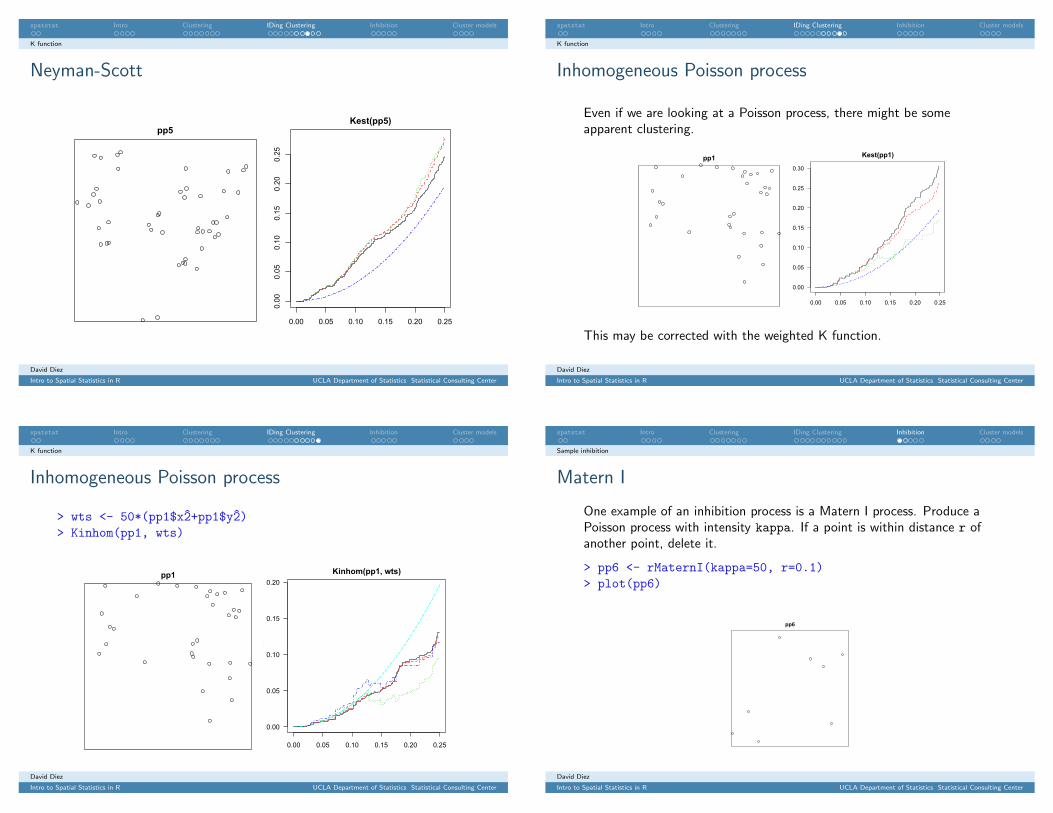
Neyman-Scott
pp5
0.00 0.05 0.10 0.15 0.20 0.25
0.00
0.05
0.10
0.15
0.20
0.25
Kest(pp5)
K(r)
David Diez
Intro to Spatial Statistics in R UCLA Department of Statistics Statistical Consulting Center
spatstat Intro Clustering IDing Clustering Inhibition Cluster models
K function
Inhomogeneous Poisson process
Even if we are looking at a Poisson process, there might be someapparent clustering.
pp1
0.00 0.05 0.10 0.15 0.20 0.25
0.00
0.05
0.10
0.15
0.20
0.25
0.30
Kest(pp1)
K(r)
This may be corrected with the weighted K function.
David Diez
Intro to Spatial Statistics in R UCLA Department of Statistics Statistical Consulting Center
spatstat Intro Clustering IDing Clustering Inhibition Cluster models
K function
Inhomogeneous Poisson process
> wts <- 50*(pp1$x2̂+pp1$y2̂)> Kinhom(pp1, wts)
pp1
0.00 0.05 0.10 0.15 0.20 0.25
0.00
0.05
0.10
0.15
0.20Kinhom(pp1, wts)
Kinhom(r)
David Diez
Intro to Spatial Statistics in R UCLA Department of Statistics Statistical Consulting Center
spatstat Intro Clustering IDing Clustering Inhibition Cluster models
Sample inhibition
Matern I
One example of an inhibition process is a Matern I process. Produce aPoisson process with intensity kappa. If a point is within distance r ofanother point, delete it.
> pp6 <- rMaternI(kappa=50, r=0.1)> plot(pp6)
pp6
David Diez
Intro to Spatial Statistics in R UCLA Department of Statistics Statistical Consulting Center
spatstat Intro Clustering IDing Clustering Inhibition Cluster models
Sample inhibition
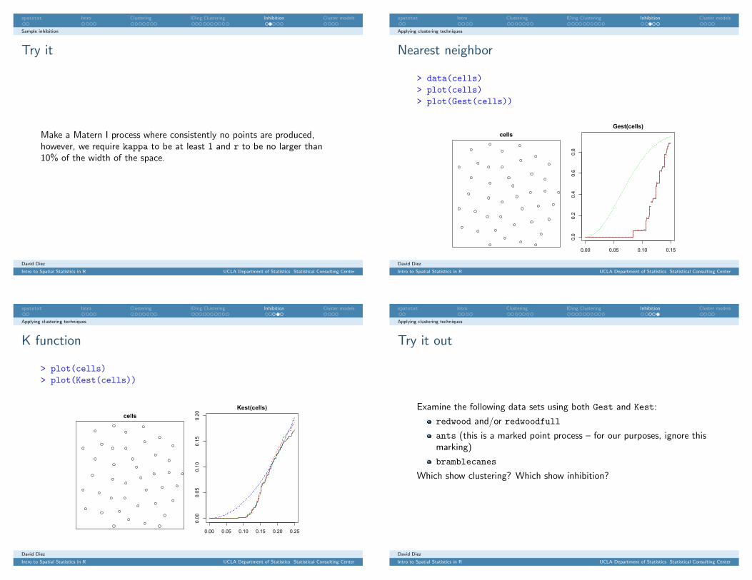
Try it
Make a Matern I process where consistently no points are produced,however, we require kappa to be at least 1 and r to be no larger than10% of the width of the space.
David Diez
Intro to Spatial Statistics in R UCLA Department of Statistics Statistical Consulting Center
spatstat Intro Clustering IDing Clustering Inhibition Cluster models
Applying clustering techniques
Nearest neighbor
> data(cells)> plot(cells)> plot(Gest(cells))
cells
0.00 0.05 0.10 0.15
0.0
0.2
0.4
0.6
0.8
Gest(cells)
G(r)
David Diez
Intro to Spatial Statistics in R UCLA Department of Statistics Statistical Consulting Center
spatstat Intro Clustering IDing Clustering Inhibition Cluster models
Applying clustering techniques
K function
> plot(cells)> plot(Kest(cells))
cells
0.00 0.05 0.10 0.15 0.20 0.25
0.00
0.05
0.10
0.15
0.20
Kest(cells)
K(r)
David Diez
Intro to Spatial Statistics in R UCLA Department of Statistics Statistical Consulting Center
spatstat Intro Clustering IDing Clustering Inhibition Cluster models
Applying clustering techniques
Try it out
Examine the following data sets using both Gest and Kest:
redwood and/or redwoodfull
ants (this is a marked point process – for our purposes, ignore thismarking)
bramblecanes
Which show clustering? Which show inhibition?
David Diez
Intro to Spatial Statistics in R UCLA Department of Statistics Statistical Consulting Center

spatstat Intro Clustering IDing Clustering Inhibition Cluster models
Model fitting
Cluster model fitting
The package spatstat offers a variety of tools that can be used toestimate parameters of particular processes. We examine the utility of acouple of the functions.
David Diez
Intro to Spatial Statistics in R UCLA Department of Statistics Statistical Consulting Center
spatstat Intro Clustering IDing Clustering Inhibition Cluster models
Examples
Matern cluster process
> pp7 <- rThomas(10,0.03,7)> thomas.estK(pp7)...kappa sigma mu
9.85002358 0.03294598 5.68526558
pp7
David Diez
Intro to Spatial Statistics in R UCLA Department of Statistics Statistical Consulting Center
spatstat Intro Clustering IDing Clustering Inhibition Cluster models
Examples
Thomas process
> pp7 <- rThomas(10,0.03,7)> thomas.estK(pp8)...kappa sigma mu
10.63830700 0.02599699 5.63999516
pp8
David Diez
Intro to Spatial Statistics in R UCLA Department of Statistics Statistical Consulting Center
spatstat Intro Clustering IDing Clustering Inhibition Cluster models
Try it
Try it
Use the two processes you used to create patterns, clearlyClusteredand littleClustered, and see how well the parameter fits are usingmatclust.estK.
How well does the model fit clearlyClustered? How well does it fitlittleClustered?
Try making a new pattern that is somewhere in between these twopatterns. Does the estimation work well?
David Diez
Intro to Spatial Statistics in R UCLA Department of Statistics Statistical Consulting Center

Resources Survey
Resources
Additional resources
The package geoR is a useful package that we did not examine. Forinformation on this package, see
www.maths.lancs.ac.uk/∼ribeiro/geoR.html
Book resource:
Applied Spatial Data Analysis with Rby Roger S. Bivand,
Edzer J. Pebesma, andVirgilio Gmez-Rubio
David Diez
Intro to Spatial Statistics in R UCLA Department of Statistics Statistical Consulting Center
Resources Survey
Survey
Please take our survey
Taking our survey to let us know what you think of mini-courses helpsimprove them for the future.
http://scc.stat.ucla.edu/survey
David Diez
Intro to Spatial Statistics in R UCLA Department of Statistics Statistical Consulting Center


