
Introduction to Digital Signal ProcessingPaolo Prandoni
LCAV - EPFL
Introduction to Digital Signal Processing – p. 1/25
Inside DSP. . .
Digital
Brings experimental data & abstract models together
Makes math very simple i.e. implementable
Signal
Measurement of a varying quantity
Experimental data (physics, electronics, astronomy, etc.)
Processing
Manipulation of the information content
Abstract model (math, computer science, etc.)
Introduction to Digital Signal Processing – p. 2/25

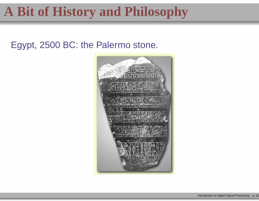
A Bit of History and Philosophy
Egypt, 2500 BC:
Introduction to Digital Signal Processing – p. 3/25
A Bit of History and Philosophy
Egypt, 2500 BC: the Palermo stone.
Introduction to Digital Signal Processing – p. 4/25
A Bit of History and Philosophy
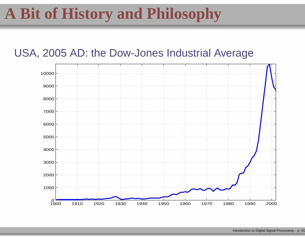
USA, 2005 AD: the Dow-Jones Industrial Average
1900 1910 1920 1930 1940 1950 1960 1970 1980 1990 20000
1000
2000
3000
4000
5000
6000
7000
8000
9000
10000
Introduction to Digital Signal Processing – p. 5/25

A Bit of History and Philosophy
What do these measurements have in common?
Life-changing phenomena
Unpredictable patterns
Discrete set of observations
= Digital Signal Processing
Is a discrete set of measurement a sufficient representation?Can we formalize this concept?
Introduction to Digital Signal Processing – p. 6/25
A Bit of History and Philosophy
The Platonic schizophrenia of Western thought.
Dichotomy between the ideal and the real
Zeno’s paradoxes
An odd synergy: calculus and ballistics
Introduction to Digital Signal Processing – p. 7/25
A Bit of History and Philosophy
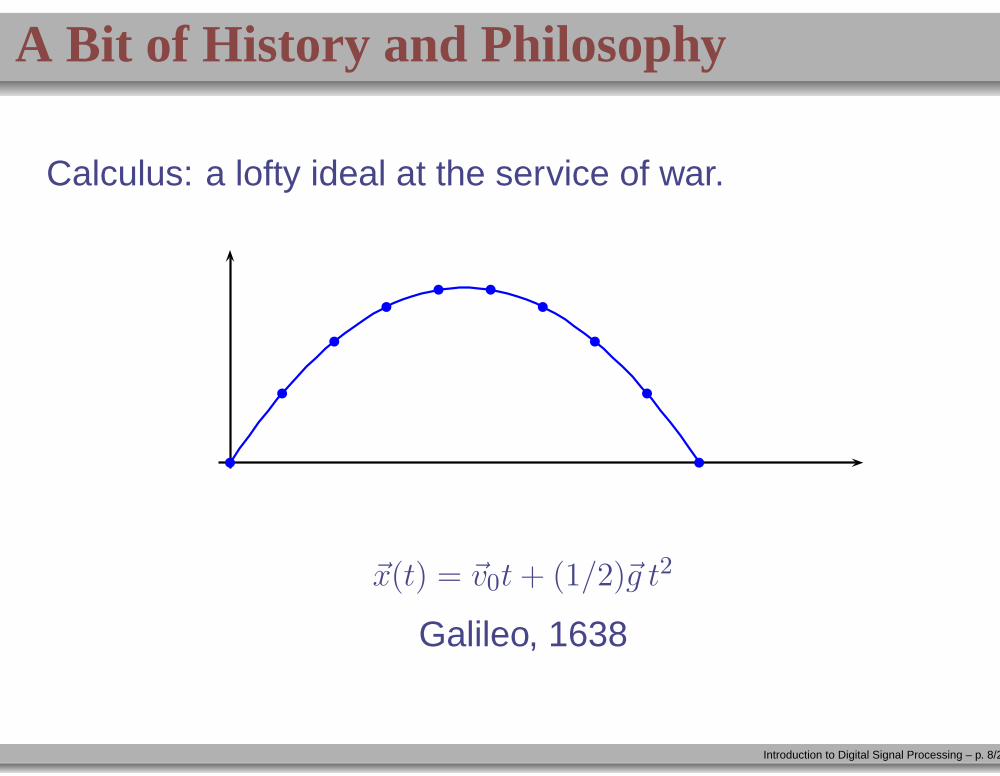
Calculus: a lofty ideal at the service of war.
b
b
b
b
b b
b
b
b
b
~x(t) = ~v0t + (1/2)~g t2
Galileo, 1638
Introduction to Digital Signal Processing – p. 8/25

Ideal Signals vs. Real Signals
How does an ideal signal look like? Tuning fork:
It’s a function of a real variable!
f(t) = A sin(2πωt + φ)
As such, 3 parameters completely describe the signal.
Introduction to Digital Signal Processing – p. 9/25

Ideal Signals vs. Real Signals
Tuning forks are boring; Bach is not:
Unfortunately (or fortunately):
f(t) =?
How do we deal with real-world signals?
Introduction to Digital Signal Processing – p. 10/25
Ideal Signals vs. Real Signals
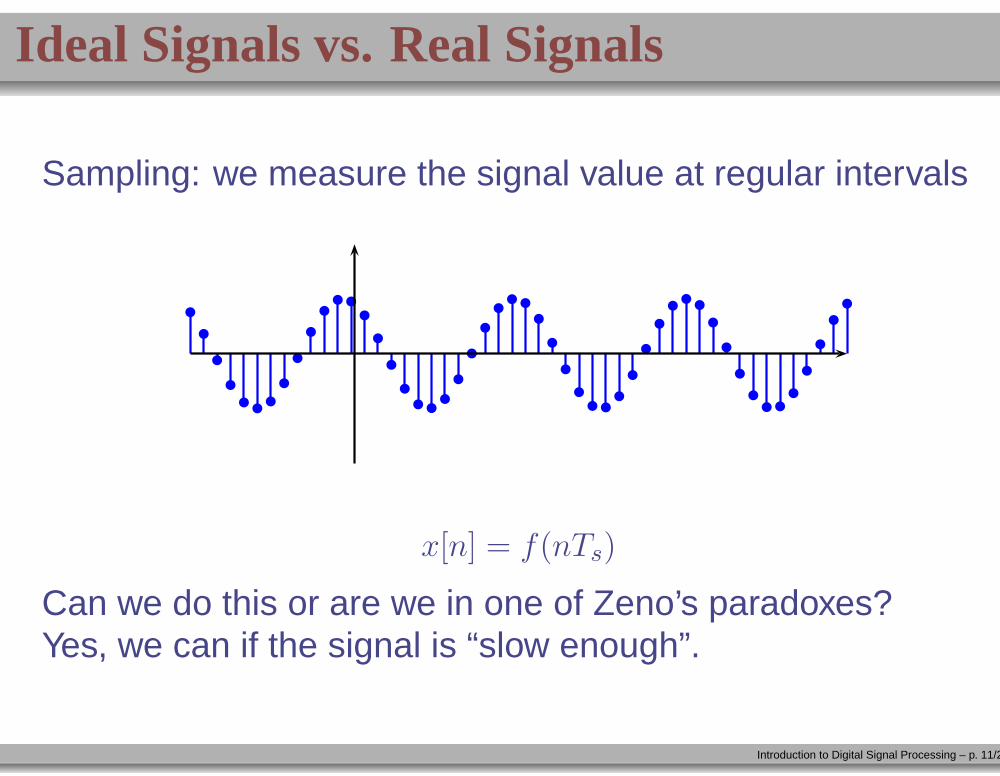
Sampling: we measure the signal value at regular intervals
b
b
b
b
bbb
b
b
b
bb b
b
b
b
b
b bb
b
b
b
bb b
b
b
b
b
b bb
b
b
b
bbb
b
b
b
bb b
b
b
b
b
b
x[n] = f(nTs)
Can we do this or are we in one of Zeno’s paradoxes?Yes, we can if the signal is “slow enough”.
Introduction to Digital Signal Processing – p. 11/25

Ideal Signals vs. Real Signals
The Sampling Theorem (Nyquist 1920).Under appropriate “slowness” conditions for f(t) we have:
f(t) =∞∑
n=−∞
x[n]sin(π(t − nTs)/Ts)
π(t − nTs)/Ts
In a way, the sampling theorem solves one of Zeno’sparadoxes: the infinite and the finite have been reconciled.
The sampling theorem is the ”revolving door” into the digital world.We will therefore operate in the digital world only.
Introduction to Digital Signal Processing – p. 12/25
The Digital Revolution
Digital signals make our life simpler:
Processing:Sequence of numbers: ideal for computations
Development easy (general-purpose hardware)
Storage:Storage is basically media-independent
Perfect duplication
Digital compression is miraculous
Communications:Transmission schemes independent of data
Error correction techniques make it noise-free
Introduction to Digital Signal Processing – p. 13/25
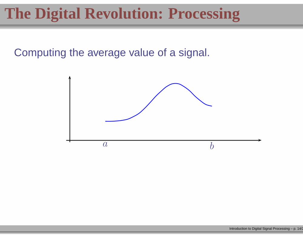
The Digital Revolution: Processing
Computing the average value of a signal.
a b
Introduction to Digital Signal Processing – p. 14/25
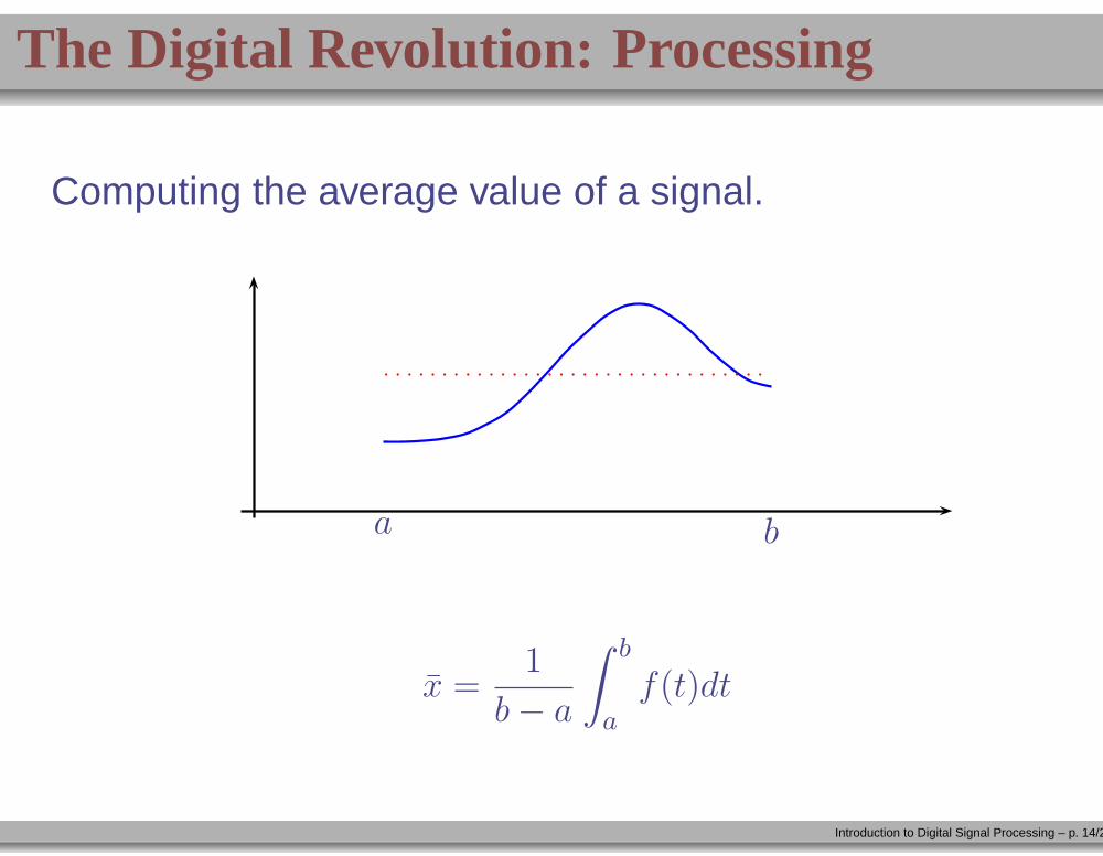
The Digital Revolution: Processing
Computing the average value of a signal.
a b
x =1
b − a
∫ b
a
f(t)dt
Introduction to Digital Signal Processing – p. 14/25
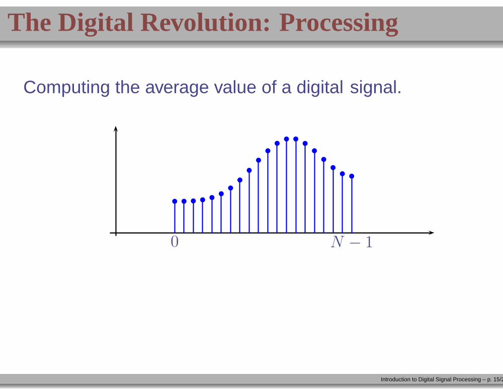
The Digital Revolution: Processing
Computing the average value of a digital signal.
b b b b bbb
b
b
b
b
bb b
b
b
b
bb b
0 N − 1
Introduction to Digital Signal Processing – p. 15/25

The Digital Revolution: Processing
Computing the average value of a digital signal.
b b b b bbb
b
b
b
b
bb b
b
b
b
bb b
0 N − 1
x =1
N
N−1∑n=0
x[n]
Introduction to Digital Signal Processing – p. 15/25

The Digital Revolution: Processing
Computing (vertical) speed the “Platonic” way.
b
b
b
b
b b
b
b
b
b
t
x(t)
x(t) = v0t − (1/2)gt2
v(t) = x(t) = v0 − gt
Introduction to Digital Signal Processing – p. 16/25
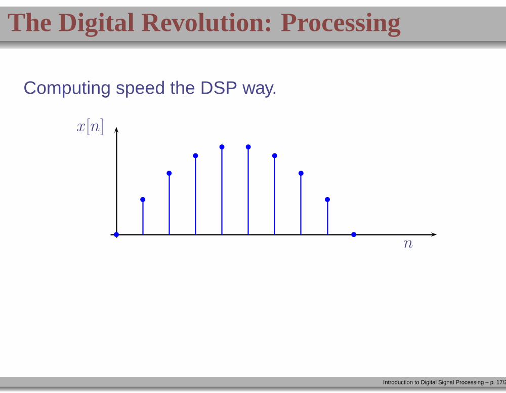
The Digital Revolution: Processing
Computing speed the DSP way.
n
x[n]
b
b
b
b
b b
b
b
b
b
Introduction to Digital Signal Processing – p. 17/25

The Digital Revolution: Processing
Computing speed the DSP way.
n
x[n]
∆x
∆T
b
b
b
b
b b
b
b
b
b
v[n] = (x[n] − x[n − 1])/Ts
Introduction to Digital Signal Processing – p. 17/25

The Digital Revolution: Processing
The ”Speed Filter”:
Position Processing Speed
Introduction to Digital Signal Processing – p. 18/25
The Digital Revolution: Processing
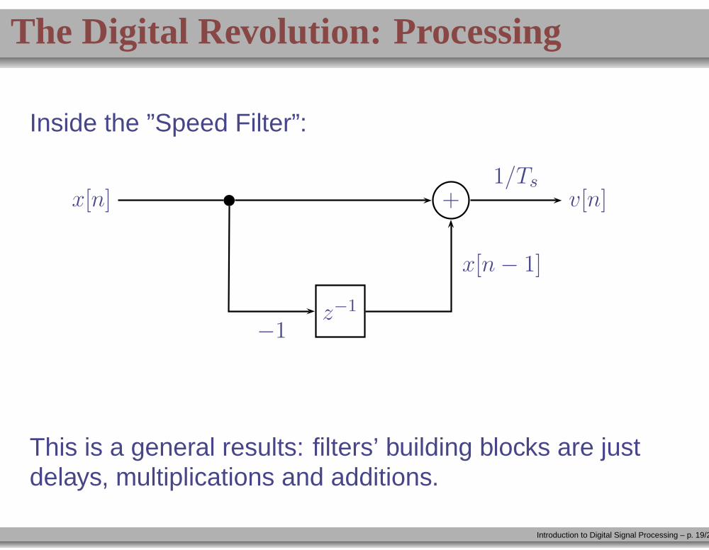
Inside the ”Speed Filter”:
x[n] +
z−1
v[n]1/Ts
x[n − 1]
−1
This is a general results: filters’ building blocks are justdelays, multiplications and additions.
Introduction to Digital Signal Processing – p. 19/25
The Digital Revolution: Storage
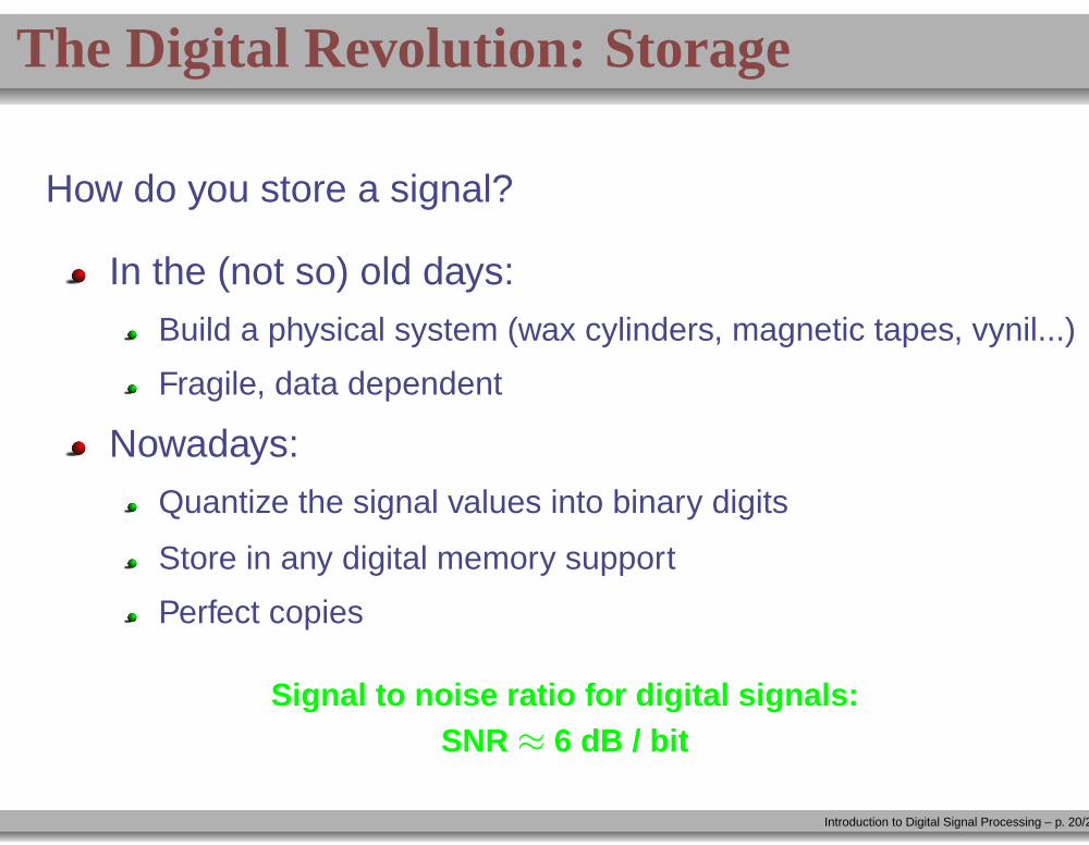
How do you store a signal?
In the (not so) old days:Build a physical system (wax cylinders, magnetic tapes, vynil...)
Fragile, data dependent
Nowadays:Quantize the signal values into binary digits
Store in any digital memory support
Perfect copies
Signal to noise ratio for digital signals:SNR ≈ 6 dB / bit
Introduction to Digital Signal Processing – p. 20/25

The Digital Revolution: Storage
How do you deal with large amounts of data? Compression!
Signal Type Default Rate Compressed Rate
Music4.32 Mbps
CD audio
128 Kbps
MP3
Voice64 Kbps
AM radio
4.8 Kbps
CELP
Image20 Mb
this image600 Kb
JPEG
Video170 Mbs
PAL video
600-800 Kbs
DiVx
Introduction to Digital Signal Processing – p. 21/25
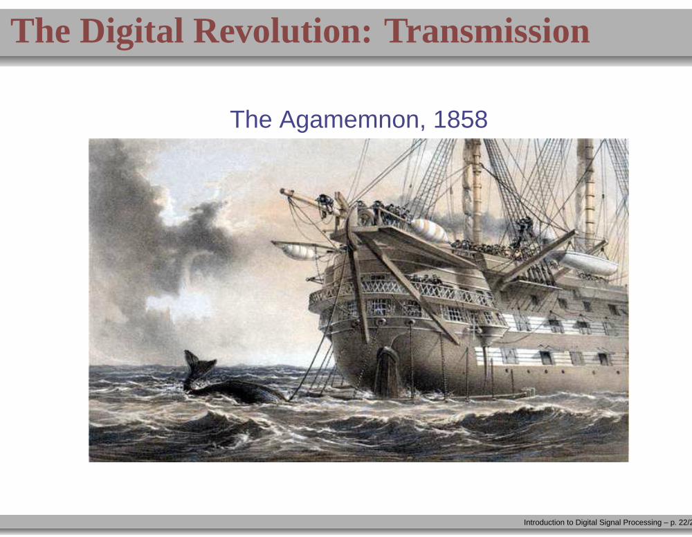
The Digital Revolution: Transmission
The Agamemnon, 1858
Introduction to Digital Signal Processing – p. 22/25

The Digital Revolution: Transmission
Digital data allows for large throughputs:
Transoceanic cable:1866: 8 words per minute (≈5 bps)
1956: AT&T, coax, 48 voice channels (≈3Mbps)
2005: Alcatel Tera10, fiber, 8.4 Tbps (1012 bps)
Introduction to Digital Signal Processing – p. 23/25

The Digital Revolution: Transmission
Digital data allows for large throughputs:
Transoceanic cable:1866: 8 words per minute (≈5 bps)
1956: AT&T, coax, 48 voice channels (≈3Mbps)
2005: Alcatel Tera10, fiber, 8.4 Tbps (1012 bps)
Voiceband modems:1950s: Bell 202, 1200 bps
1990s: V90, 56000bps
Introduction to Digital Signal Processing – p. 23/25
DSP Friends and Partners
Electronics
Computer science
Physiology
Music
Medicine
Photography
And many more...
Introduction to Digital Signal Processing – p. 24/25

Conclusions
Digital signal processing is FUN!
It’s a fresh new take on what you already studied in theory.
Just turn on a computer and you have a “mad scientist lab”where you can bring everything you know, and nothing ever
blows up.
Introduction to Digital Signal Processing – p. 25/25


![Index [application.wiley-vch.de]digital memory 114 digital mirror device 215 digital MOS circuit 53 digital power management 485 digital products 568 digital signal 55 digital technology](https://static.documents.pub/doc/80x56/5f08ef357e708231d4246eeb/index-digital-memory-114-digital-mirror-device-215-digital-mos-circuit-53-digital.jpg)


![Digital Brand and Style Guidelines...Contents Digital proposition 4 Digital users .....5 . Plan2go: Digital Brand and Style Guidelines [ 4 ] Digital proposition The Plan2go digital](https://static.documents.pub/doc/80x56/5e8b4f7b301a8c0a1263580c/digital-brand-and-style-guidelines-contents-digital-proposition-4-digital-users.jpg)