
Inventory Management
OutlineBasic Definitions and Ideas• Reasons to Hold Inventory• Inventory CostsInventory Control Systems• Continuous Review Models
• Basic EOQ Model• Quantity Discounts• Safety Stock• Special Case: The News Vendor Problem
• Discrete Probability Example• Continuous Probability Example
• Periodic Review Model

What is Inventory?
• Inventory is a stock of items held to meet future demand.
• Inventory management answers two questions:– How much to order– When to order
Basic Concepts of Inventory Management can be expanded to apply to a broad array of types of “inventory”:
– Raw materials– Purchased parts and supplies– Labor– In-process (partially completed)
products– Component parts– Working capital– Tools, machinery, and equipment– Finished goods
Reasons to Hold Inventory
• Meet unexpected demand• Smooth seasonal or cyclical
demand• Meet variations in customer
demand• Take advantage of price discounts• Hedge against price increases• Quantity discounts
Two Forms of Demand
• Dependent– items used to produce final products
• Independent– items demanded by external
customers
Inventory Costs
• Carrying Cost– cost of holding an item in inventory
• Ordering Cost– cost of replenishing inventory
• Shortage Cost– temporary or permanent loss of sales
when demand cannot be met
Inventory Control Systems
• Fixed-order-quantity system (Continuous)– constant amount ordered when
inventory declines to predetermined level
• Fixed-time-period system (Periodic)– order placed for variable amount after
fixed passage of time
Continuous Review Models
• Basic EOQ Model• Quantity Discounts• Safety Stock
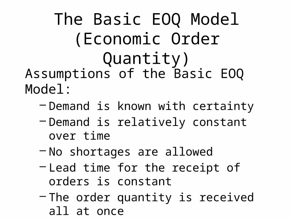
The Basic EOQ Model(Economic Order Quantity)
Assumptions of the Basic EOQ Model:
– Demand is known with certainty – Demand is relatively constant over
time– No shortages are allowed– Lead time for the receipt of orders is
constant– The order quantity is received all at
once
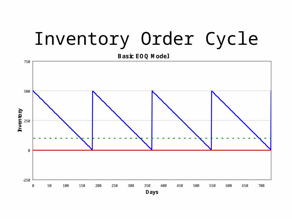
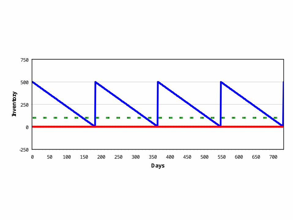
Inventory Order CycleBasic EOQ Model
-250
0
250
500
750
0 50 100 150 200 250 300 350 400 450 500 550 600 650 700
Days
Inve
nto
ry

EOQ Model Costs
S = cost of placing order D = annual demand
H = annual per-unit carrying cost Q = order quantity
Annual ordering cost = SD/ Q Annual carrying cost = HQ/ 2
Total cost = SD/ Q + HQ/ 2 Q* = Economic Order Quantity

EOQ Cost CurvesEOQ Example
0
250
500
750
1000
0 100 200 300 400 500 600 700 800 900 1000
Order Quantity
To
tal A
nn
ua
l Co
st OrderingHoldingTotal
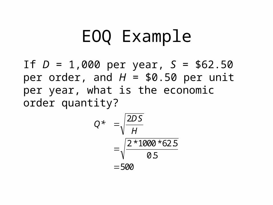
EOQ Example
If D = 1,000 per year, S = $62.50 per order, and H = $0.50 per unit per year, what is the economic order quantity?
Q* HDS2
5.0
5.62*1000*2
500

Quantity DiscountsPrice per unit decreases as order quantity increases:
Quantity Price 1-49 $35.00 50-74 $34.75 75-149 $33.55 150-299 $32.35 300-499 $31.15 500+ $30.75

Quantity Discount Costs
demand annual=
priceunit per2
D
C
CDQH
QDS
TC
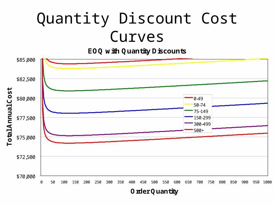
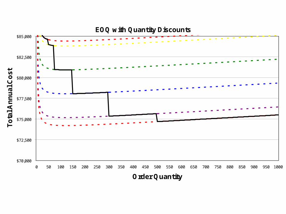
Quantity Discount Cost Curves
EOQ with Quantity Discounts
$70,000
$72,500
$75,000
$77,500
$80,000
$82,500
$85,000
0 50 100 150 200 250 300 350 400 450 500 550 600 650 700 750 800 850 900 950 1000
Order Quantity
To
tal A
nn
ual
Co
st
0-4950-7475-149150-299300-499500+

Quantity Discount Algorithm
Step 1. Calculate a value for Q*.Step 2: For any discount, if the order
quantity is too low to qualify for the discount, adjust Q upward to the lowest feasible quantity.
Step 3: Calculate the total annual cost for each Q*.

Quantity Discount Algorithm
Step 1. Calculate a value for Q*.
Q* HDS2
33.3
10*400,2*2
120

Quantity Discount Algorithm
Step 2: For any discount, if the order quantity is too low to qualify for the discount, adjust Q* upward to the lowest feasible quantity.
Quantity Price Min Q* Adj. Q* 1-49 $35.00 1 120 120 50-74 $34.75 50 120 120 75-149 $33.55 75 120 120 150-299 $32.35 150 120 150 300-499 $31.15 300 120 300 500+ $30.75 500 120 500

EOQ with Quantity Discounts
$70,000
$72,500
$75,000
$77,500
$80,000
$82,500
$85,000
0 50 100 150 200 250 300 350 400 450 500 550 600 650 700 750 800 850 900 950 1000
Order Quantity
To
tal A
nn
ual
Co
st
0-4950-7475-149150-299300-499500+

Quantity Discount Algorithm
Step 3: Calculate the total annual cost for each Q*.
Quantity Price Min Q* Adj. Q* Holding Cost Ordering Cost Purchasing Cost Total Cost 1-49 $35.00 1 120 120 $ 199.90 $ 199.90 $ 84,000.00 $84,399.80 50-74 $34.75 50 120 120 $ 199.90 $ 199.90 $ 83,400.00 $83,799.80 75-149 $33.55 75 120 120 $ 199.90 $ 199.90 $ 80,520.00 $80,919.80 150-299 $32.35 150 120 150 $ 249.75 $ 160.00 $ 77,640.00 $78,049.75 300-499 $31.15 300 120 300 $ 499.50 $ 80.00 $ 74,760.00 $75,339.50 500+ $30.75 500 120 500 $ 832.50 $ 48.00 $ 73,800.00 $74,680.50
EOQ with Quantity Discounts
$70,000
$72,500
$75,000
$77,500
$80,000
$82,500
$85,000
0 50 100 150 200 250 300 350 400 450 500 550 600 650 700 750 800 850 900 950 1000
Order Quantity
To
tal
An
nu
al C
ost
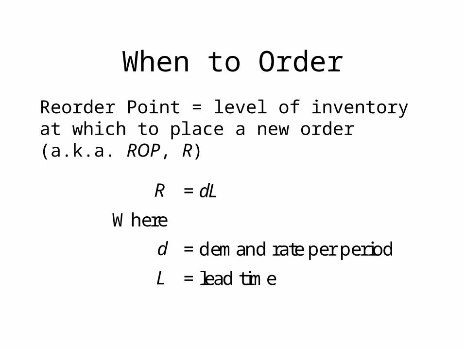
When to Order
Reorder Point = level of inventory at which to place a new order (a.k.a. ROP, R)
R = dL
Where
d = demand rate per period
L = lead time
-250
0
250
500
750
0 50 100 150 200 250 300 350 400 450 500 550 600 650 700
Days
Inve
nto
ry
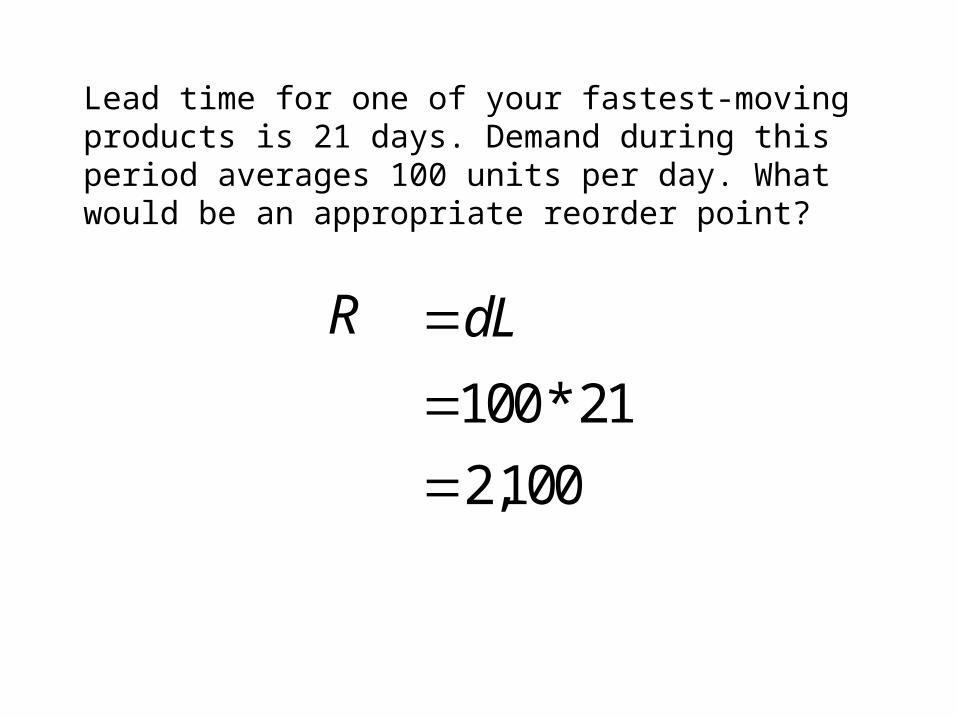
Lead time for one of your fastest-moving products is 21 days. Demand during this period averages 100 units per day. What would be an appropriate reorder point?
R dL
21*100
100,2
-1000
-500
0
500
1000
1500
2000
2500
3000
3500
4000
0 50 100 150 200 250 300 350
Days
Inv
en
tory
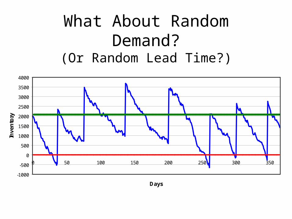
What About Random Demand?
(Or Random Lead Time?)
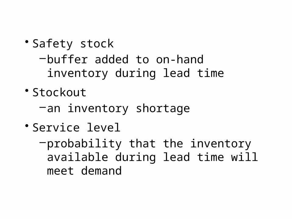
• Safety stock–buffer added to on-hand inventory
during lead time
• Stockout –an inventory shortage
• Service level –probability that the inventory
available during lead time will meet demand

Reorder Point with Variable Demand
(Leadtime is Constant)
stocksafetyz
z
L
d
zLdR
d
level service desired for deviations standard of number=
time lead during demand ofdeviation standard
demand daily ofdeviation standard
time lead=
demand daily average=
where,
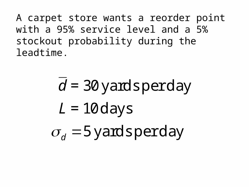
A carpet store wants a reorder point with a 95% service level and a 5% stockout probability during the leadtime.
day per yards 5
days 10=
day per yards 30=
d
L
d
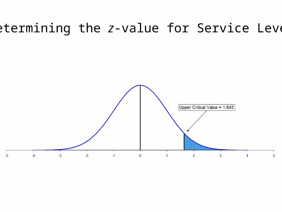
Determining the z-value for Service Level
L=
L=
L=
=
d
2d
2d
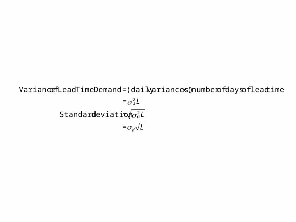
deviation Standard
time) lead of days of (number x variances) (dailyDemand Time Lead of Variance

yards 1.26)10)(5)(65.1(stock Safety
yards 1.3261.26300)10)(5)(65.1()10)(30(
day per yards 5
days 10=
day per yards 30=
z
zLdR
L
d
d
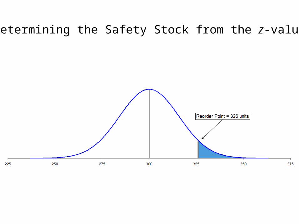
Determining the Safety Stock from the z-value

What If Leadtime is Random?
Random Variable Mean Standard Deviation
L = Leadtime L L
d = Demand d d
dL = Demand during Leadtime Ld 222Ld dL

Special Case: The Newsboy Problem
The News Vendor Problem is a special “single period” version of the EOQ model, where the product drops in value after a relatively brief selling period. The name comes from newspapers, which are much less valuable after the day they are originally published. This model may be useful for any product with a short product life cycle, such as • Time-sensitive Materials (newspapers,
magazines)• Fashion Goods (some kinds of apparel)• Perishable Goods (some food products)
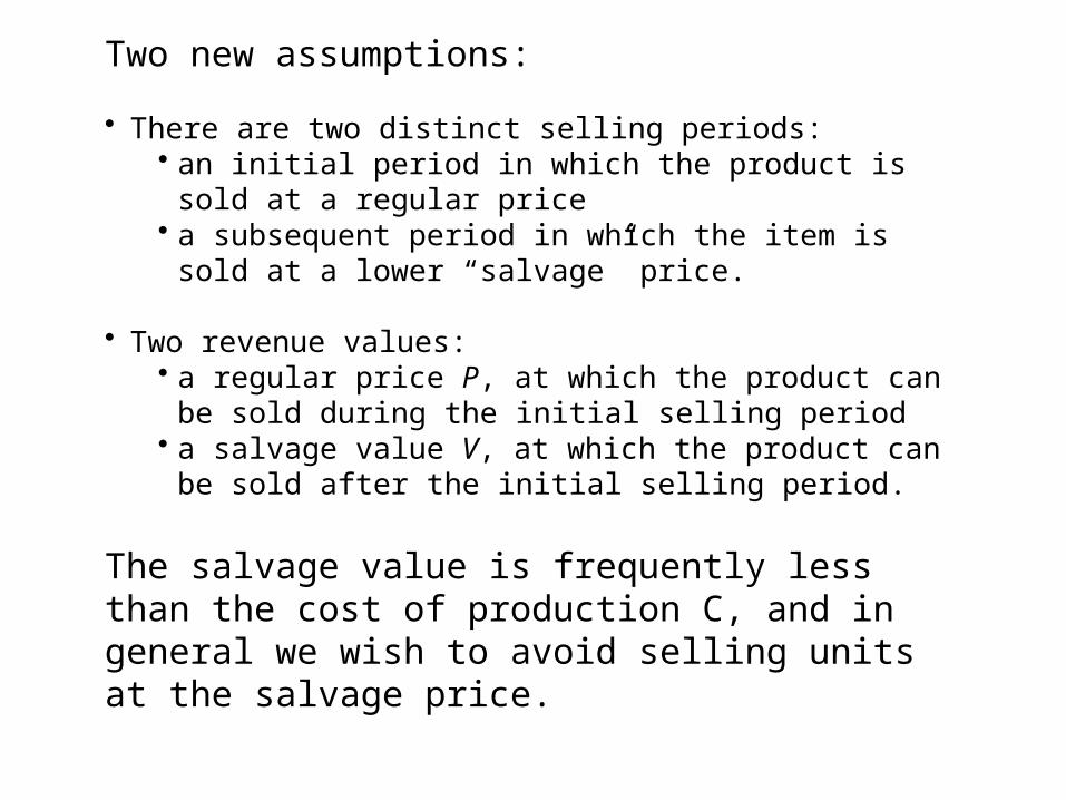
Two new assumptions:
• There are two distinct selling periods: • an initial period in which the product is sold at a
regular price• a subsequent period in which the item is sold at a
lower “salvage” price.
• Two revenue values: • a regular price P, at which the product can be sold
during the initial selling period• a salvage value V, at which the product can be sold
after the initial selling period.
The salvage value is frequently less than the cost of production C, and in general we wish to avoid selling units at the salvage price.
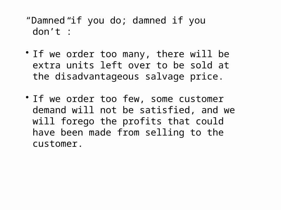
“Damned if you do; damned if you don’t”: • If we order too many, there will be extra
units left over to be sold at the disadvantageous salvage price.
• If we order too few, some customer demand will not be satisfied, and we will forego the profits that could have been made from selling to the customer.
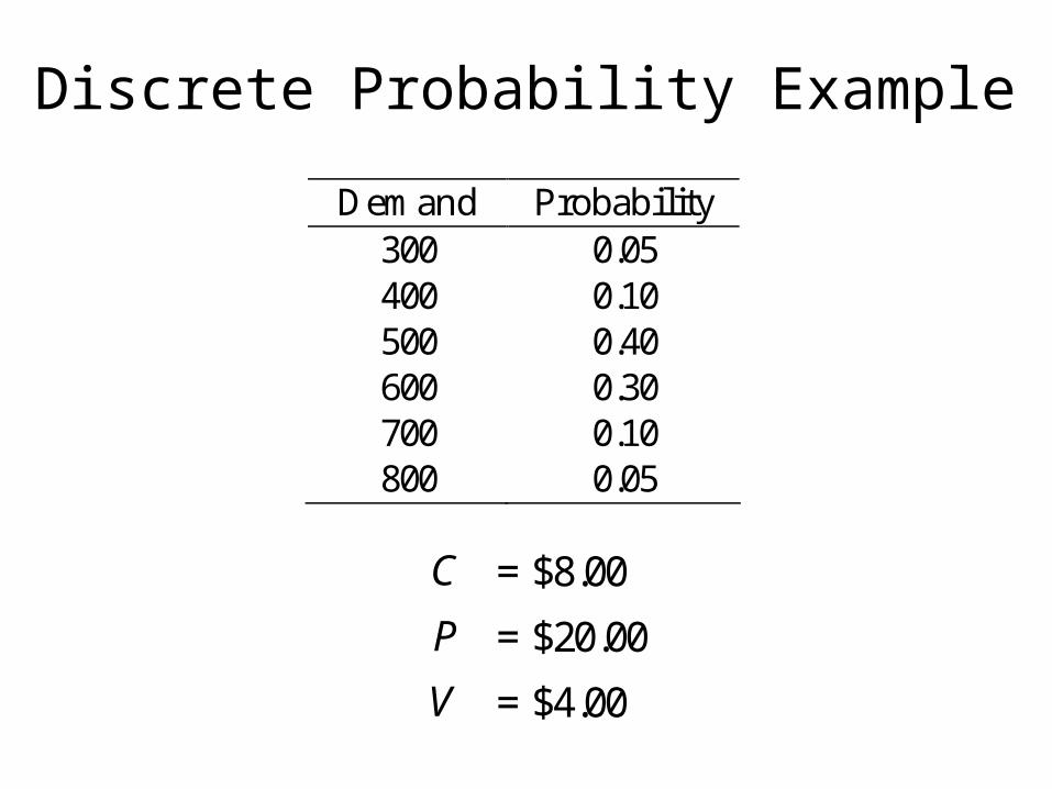
C = $8.00
P = $20.00
V = $4.00
Demand Probability 300 0.05 400 0.10 500 0.40 600 0.30 700 0.10 800 0.05
Discrete Probability Example
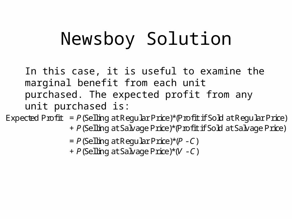
Newsboy Solution
In this case, it is useful to examine the marginal benefit from each unit purchased. The expected profit from any unit purchased is:
Expected Profit = P(Selling at Regular Price)*(Profit if Sold at Regular Price) + P(Selling at Salvage Price)*(Profit if Sold at Salvage Price)
= P(Selling at Regular Price)*(P - C) + P(Selling at Salvage Price)*(V - C)
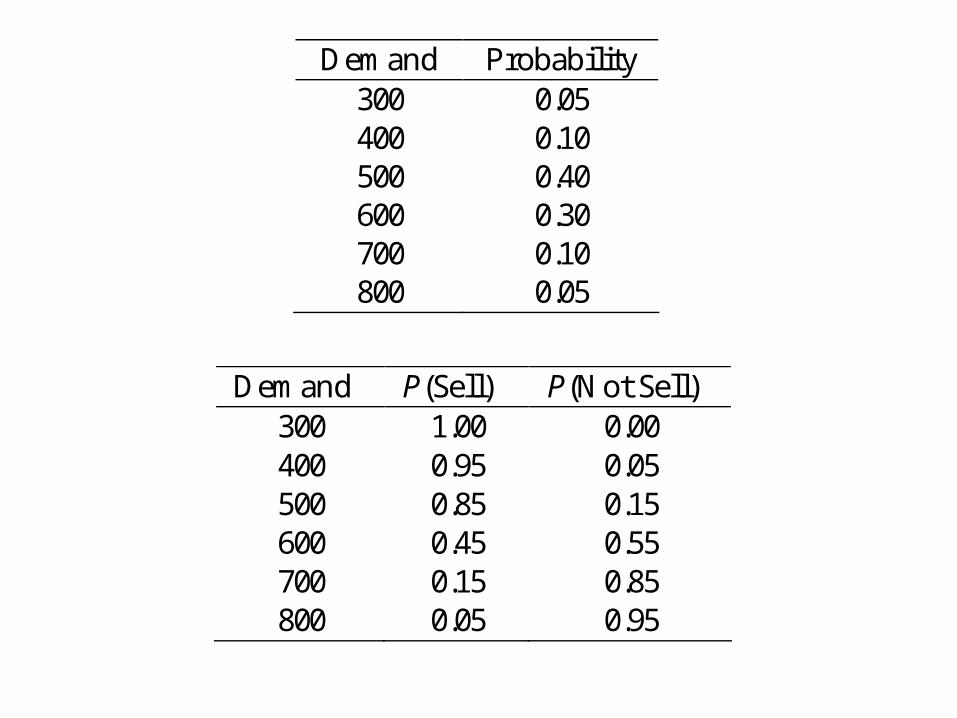
Demand Probability 300 0.05 400 0.10 500 0.40 600 0.30 700 0.10 800 0.05
Demand P(Sell) P(Not Sell) 300 1.00 0.00 400 0.95 0.05 500 0.85 0.15 600 0.45 0.55 700 0.15 0.85 800 0.05 0.95

Demand Prob. P(Sell) Profit if Sold P(Not Sell) Profit if Not Sold Weighted Average Profit 300 0.05 1.00 $ 12.00 0.00 $ (4.00) $ 12.00 400 0.10 0.95 $ 12.00 0.05 $ (4.00) $ 11.20 500 0.40 0.85 $ 12.00 0.15 $ (4.00) $ 9.60 600 0.30 0.45 $ 12.00 0.55 $ (4.00) $ 3.20 700 0.10 0.15 $ 12.00 0.85 $ (4.00) $ (1.60) 800 0.05 0.05 $ 12.00 0.95 $ (4.00) $ (3.20)
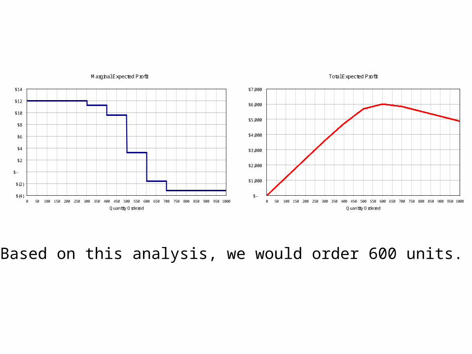
Based on this analysis, we would order 600 units.
Marginal Expected Profit
$(4)
$(2)
$-
$2
$4
$6
$8
$10
$12
$14
0 50 100 150 200 250 300 350 400 450 500 550 600 650 700 750 800 850 900 9501000
Quantity Ordered
Total Expected Profit
$-
$1,000
$2,000
$3,000
$4,000
$5,000
$6,000
$7,000
0 50 100 150 200 250 300 350 400 450 500 550 600 650 700 750 800 850 900 9501000
Quantity Ordered

Continuous Probability Example
Using the same mean and standard deviation as in the previous case (545.0 and 111.7), what would be optimal if demand were normally distributed?

Define CO and CU to be the “costs” of over-ordering and under-ordering, respectively.
In this case: CO CV
84
00.4$
CU CP
820
00.12$

It can be shown that the optimal order quantity is the value in the demand distribution that corresponds to the “critical probability”:
Critical probability OU
U
CCC
412
12
1612
75.0
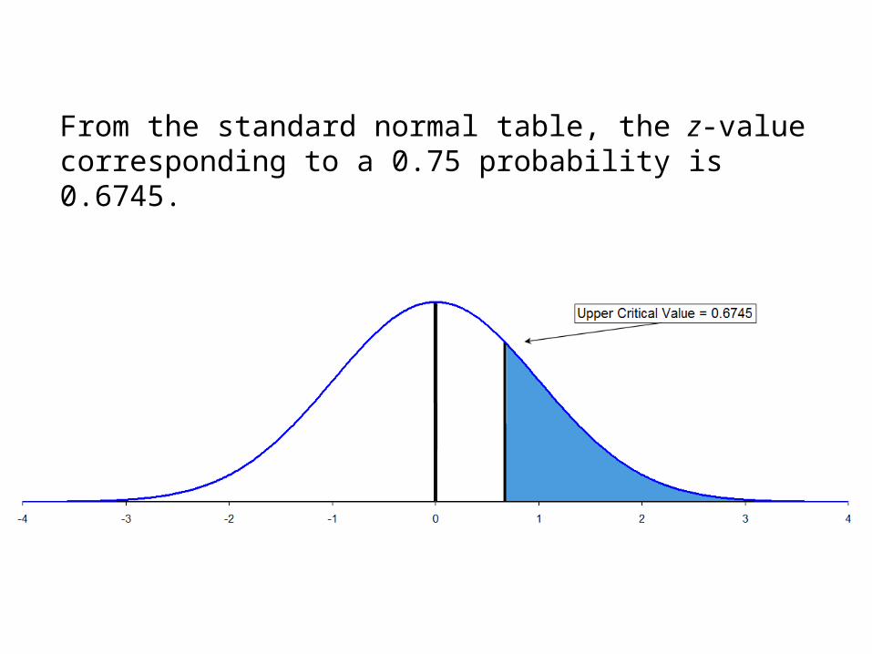
From the standard normal table, the z-value corresponding to a 0.75 probability is 0.6745.
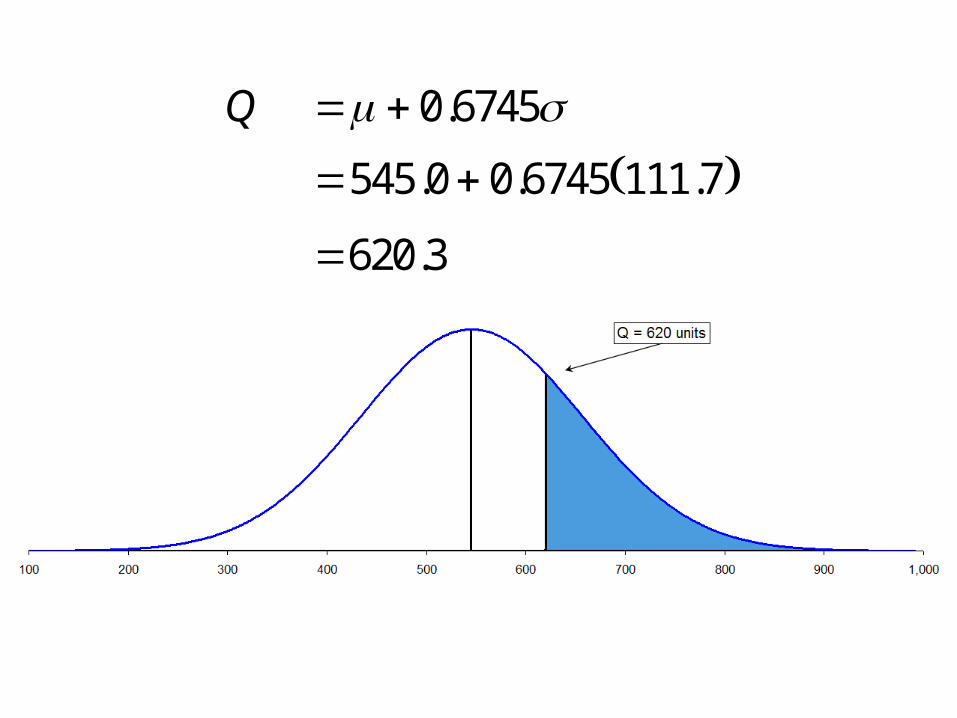
Q 6745.0
7.1116745.00.545
3.620

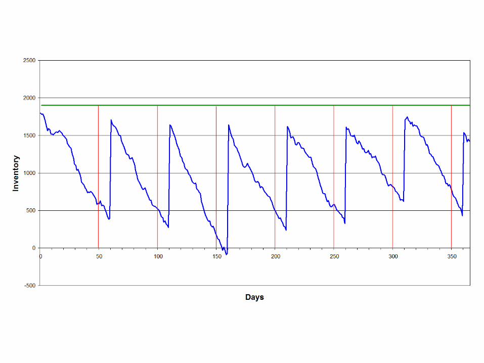
Periodic Review Models
Sometimes a continuous review system doesn’t make sense, as when the item is not very expensive to carry, and/or when the customers don’t mind waiting for a backorder. A periodic review system only checks inventory and places orders at fixed intervals of time.
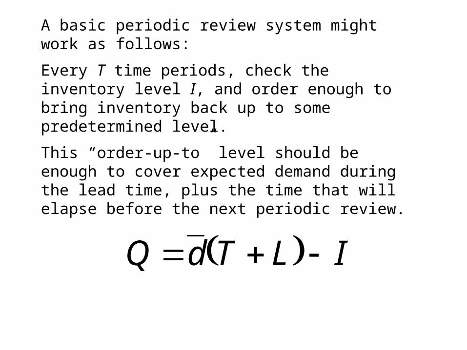
A basic periodic review system might work as follows:
Every T time periods, check the inventory level I, and order enough to bring inventory back up to some predetermined level.
This “order-up-to” level should be enough to cover expected demand during the lead time, plus the time that will elapse before the next periodic review.
ILTdQ

We might also build some safety stock in to the “order-up-to” quantity.
IzLTdQ LT
B01.2314 -- Operations -- Prof. Juran
53
What is Supply-Chain Management?
Supply-chain management is a total system approach to managing the entire flow of information, materials, and services from raw-material suppliers through factories and warehouses to the end customer
B01.2314 -- Operations -- Prof. Juran
54
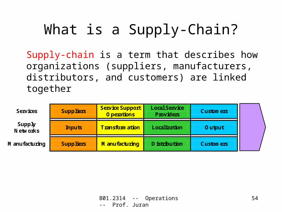
What is a Supply-Chain?
Supply-chain is a term that describes how organizations (suppliers, manufacturers, distributors, and customers) are linked together
Services Suppliers Service Support
Operations Local Service
Providers Customers
Supply Networks
Inputs Transformation Localization Output
Manufacturing Suppliers Manufacturing Distribution Customers
B01.2314 -- Operations -- Prof. Juran
55
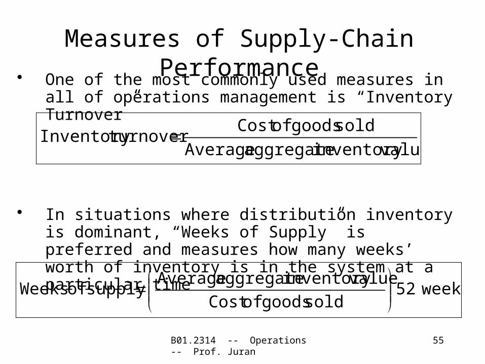
Measures of Supply-Chain Performance• One of the most commonly used measures in all of
operations management is “Inventory Turnover”
• In situations where distribution inventory is dominant, “Weeks of Supply” is preferred and measures how many weeks’ worth of inventory is in the system at a particular time
valueinventory aggregate Average
sold goods ofCost turnoverInventory
weeks52 sold goods ofCost
valueinventory aggregate Averagesupply of Weeks
B01.2314 -- Operations -- Prof. Juran
56
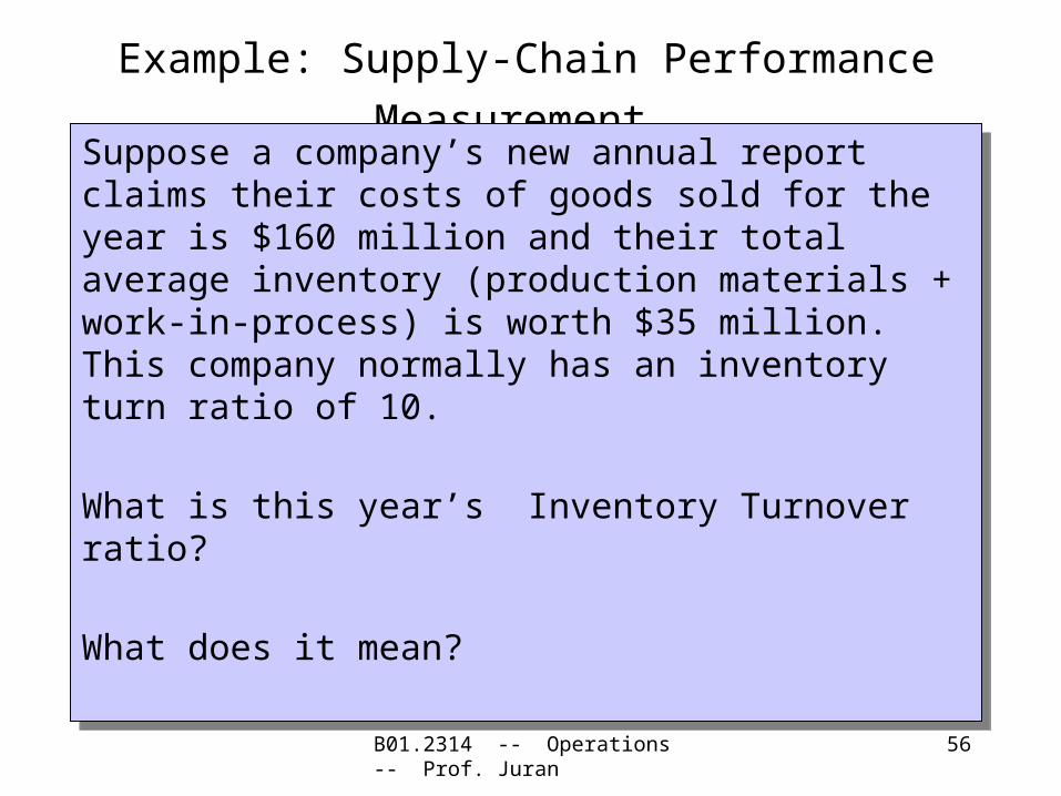
Example: Supply-Chain Performance
Measurement Suppose a company’s new annual report claims their costs of goods sold for the year is $160 million and their total average inventory (production materials + work-in-process) is worth $35 million. This company normally has an inventory turn ratio of 10.
What is this year’s Inventory Turnover ratio?
What does it mean?
Suppose a company’s new annual report claims their costs of goods sold for the year is $160 million and their total average inventory (production materials + work-in-process) is worth $35 million. This company normally has an inventory turn ratio of 10.
What is this year’s Inventory Turnover ratio?
What does it mean?

B01.2314 -- Operations -- Prof. Juran
57
valueinventory aggregate Average
sold goods ofCost turnoverInventory
123
A B CCOGS 160,000,000$ Avg Inventory 35,000,000$ Turnover 4.57
=B1/B2
B01.2314 -- Operations -- Prof. Juran
58
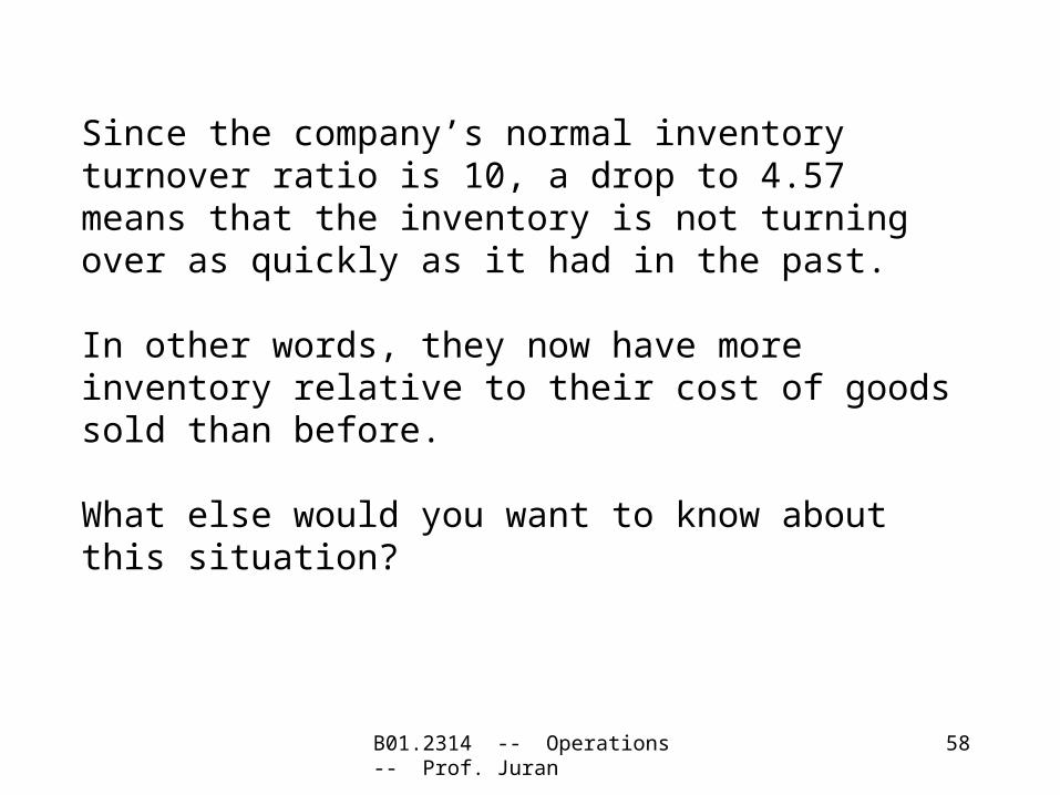
Since the company’s normal inventory turnover ratio is 10, a drop to 4.57 means that the inventory is not turning over as quickly as it had in the past.
In other words, they now have more inventory relative to their cost of goods sold than before.
What else would you want to know about this situation?

B01.2314 -- Operations -- Prof. Juran
59
Supply Chain Strategy
Marshall Fisher:• Adverse effects of price
promotions• Functional vs. Innovative products
B01.2314 -- Operations -- Prof. Juran
60
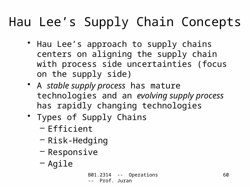
Hau Lee’s Supply Chain Concepts
• Hau Lee’s approach to supply chains centers on aligning the supply chain with process side uncertainties (focus on the supply side)
• A stable supply process has mature technologies and an evolving supply process has rapidly changing technologies
• Types of Supply Chains– Efficient– Risk-Hedging– Responsive– Agile
B01.2314 -- Operations -- Prof. Juran
61
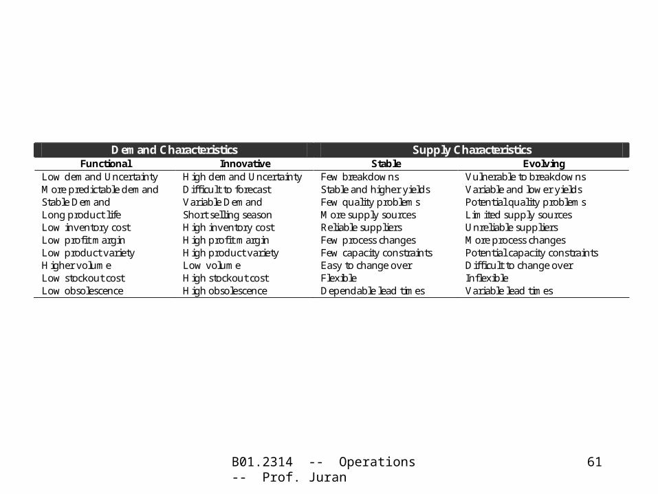
Demand Characteristics Supply Characteristics Functional Innovative Stable Evolving
Low demand Uncertainty High demand Uncertainty Few breakdowns Vulnerable to breakdowns More predictable demand Difficult to forecast Stable and higher yields Variable and lower yields Stable Demand Variable Demand Few quality problems Potential quality problems Long product life Short selling season More supply sources Limited supply sources Low inventory cost High inventory cost Reliable suppliers Unreliable suppliers Low profit margin High profit margin Few process changes More process changes Low product variety High product variety Few capacity constraints Potential capacity constraints Higher volume Low volume Easy to change over Difficult to change over Low stockout cost High stockout cost Flexible Inflexible Low obsolescence High obsolescence Dependable lead times Variable lead times
B01.2314 -- Operations -- Prof. Juran
62
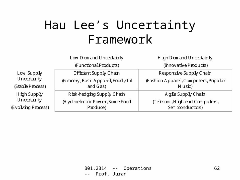
Hau Lee’s Uncertainty Framework
Low Demand Uncertainty
(Functional Products)
High Demand Uncertainty
(Innovative Products)
Low Supply Uncertainty
(Stable Process)
Efficient Supply Chain
(Grocery, Basic Apparel, Food, Oil and Gas)
Responsive Supply Chain
(Fashion Apparel, Computers, Popular Music)
High Supply Uncertainty
(Evolving Process)
Risk-hedging Supply Chain
(Hydroelectric Power, Some Food Produce)
Agile Supply Chain
(Telecom, High-end Computers, Semiconductors)

B01.2314 -- Operations -- Prof. Juran
63
Value Density
• Value density is defined as the value of an item per pound of weight
• An important measure when deciding where items should be stocked geographically and how they should be shipped
B01.2314 -- Operations -- Prof. Juran
64
Mass Customization
• Mass customization is a term used to describe the ability of a company to deliver highly customized products and services to different customers
• The key to mass customization is effectively postponing the tasks of differentiating a product for a specific customer until the latest possible point in the supply-chain network

B01.2314 -- Operations -- Prof. Juran
65
Mass Customization• Principle 1: A product should be
designed so it consists of independent modules that can be assembled into different forms of the product easily and inexpensively.
• Principle 2: Manufacturing and service processes should be designed so that they consist of independent modules that can be moved or rearranged easily to support different distribution network strategies.

B01.2314 -- Operations -- Prof. Juran
66
Mass Customization
• Principle 3: The supply network — the positioning of the inventory and the location, number, and structure of service, manufacturing, and distribution facilities — should be designed to provide two capabilities. First, it must be able to supply the basic product to the facilities performing the customization in a cost-effective manner. Second, it must have the flexibility and the responsiveness to take individual customers’ orders and deliver the finished, customized good quickly.

B01.2314 -- Operations -- Prof. Juran
67
Summary
• Supply-Chain Management• Measuring Supply-Chain Performance• Outsourcing• Value Density• Mass Customization
SummaryBasic Definitions and Ideas• Reasons to Hold Inventory• Inventory CostsInventory Control Systems• Continuous Review Models
• Basic EOQ Model• Quantity Discounts• Safety Stock• Special Case: The News Vendor Problem
• Discrete Probability Example• Continuous Probability Example
• Periodic Review Model


