

HESSD12, 2155–2199, 2015
Inverse modelling ofin situ soil water
dynamics
B. Scharnagl et al.
Title Page
Abstract Introduction
Conclusions References
Tables Figures
J I
J I
Back Close
Full Screen / Esc
Printer-friendly Version
Interactive Discussion
Discussion
Paper
|D
iscussionP
aper|
Discussion
Paper
|D
iscussionP
aper|
Hydrol. Earth Syst. Sci. Discuss., 12, 2155–2199, 2015www.hydrol-earth-syst-sci-discuss.net/12/2155/2015/doi:10.5194/hessd-12-2155-2015© Author(s) 2015. CC Attribution 3.0 License.
This discussion paper is/has been under review for the journal Hydrology and Earth SystemSciences (HESS). Please refer to the corresponding final paper in HESS if available.
Inverse modelling of in situ soil waterdynamics: accounting forheteroscedastic, autocorrelated, andnon-Gaussian distributed residualsB. Scharnagl1, S. C. Iden2, W. Durner2, H. Vereecken3, and M. Herbst3
1Department of Soil Physics, Helmholtz-Zentrum für Umweltforschung – UFZ,06102 Halle, Germany2Institute of Geoecology, Technische Universität Braunschweig,38106 Braunschweig, Germany3Agrosphere Institute (IBG-3), Forschungszentrum Jülich, 52425 Jülich, Germany
Received: 26 January 2015 – Accepted: 3 February 2015 – Published: 19 February 2015
Correspondence to: B. Scharnagl ([email protected])
Published by Copernicus Publications on behalf of the European Geosciences Union.
2155

HESSD12, 2155–2199, 2015
Inverse modelling ofin situ soil water
dynamics
B. Scharnagl et al.
Title Page
Abstract Introduction
Conclusions References
Tables Figures
J I
J I
Back Close
Full Screen / Esc
Printer-friendly Version
Interactive Discussion
Discussion
Paper
|D
iscussionP
aper|
Discussion
Paper
|D
iscussionP
aper|
Abstract
Inverse modelling of in situ soil water dynamics is a powerful tool to test process un-derstanding and determine soil hydraulic properties at the scale of interest. The ob-servations of soil water state variables are typically evaluated using the ordinary leastsquares approach. However, the underlying assumptions of this classical statistical ap-5
proach of independent, homoscedastic, and Gaussian distributed residuals are rarelytested in practice. In this case study, we estimated the soil hydraulic properties of ahomogeneous, bare soil profile from field observations of soil water contents. We useda formal Bayesian approach to estimate the posterior distribution of the parameters inthe van Genuchten–Mualem (VGM) model of the soil hydraulic properties. Three like-10
lihood models that differ with respect to assumptions about the statistical features ofthe time series of residuals were used. Our results show that the assumptions of theordinary least squares did not hold, because the residuals were strongly autocorre-lated, heteroscedastic and non-Gaussian distributed. From a statistical point of view,the parameter estimates obtained with this classical statistical approach are there-15
fore invalid. Since a test of the classic first-order autoregressive (AR(1)) model led tostrongly biased model predictions, we introduced an modified AR(1) model which elim-inates this critical deficit of the classic AR(1) scheme. The resulting improved likelihoodmodel, which additionally accounts for heteroscedasticity and nonnormality, lead to acorrect statistical characterization of the residuals and thus outperformed the other two20
likelihood models. We consider the corresponding parameter estimates as statisticallycorrect and showed that they differ systematically from those obtained under ordinaryleast squares assumptions. Moreover, the uncertainty in the parameter estimates wasincreased by accounting for autocorrelation in the observations. Our results suggestthat formal Bayesian inference using a likelihood model that correctly formalizes the25
statistical properties of the residuals may also prove useful in other inverse modellingapplications in soil hydrology.
2156

HESSD12, 2155–2199, 2015
Inverse modelling ofin situ soil water
dynamics
B. Scharnagl et al.
Title Page
Abstract Introduction
Conclusions References
Tables Figures
J I
J I
Back Close
Full Screen / Esc
Printer-friendly Version
Interactive Discussion
Discussion
Paper
|D
iscussionP
aper|
Discussion
Paper
|D
iscussionP
aper|
1 Introduction
Modelling of in situ soil water dynamics requires knowledge of the soil hydraulic proper-ties that characterize the soil at the site of interest. Various methods have been devel-oped to determine the soil hydraulic properties on soil samples taken to the laboratory.Among these laboratory methods, the multi-step outflow method (van Dam et al., 1994;5
Durner and Iden, 2011) and the evaporation method (Šimůnek et al., 1998; Peters andDurner, 2008) have found widespread application because they allow for the deter-mination of both the soil water retention function and the soil hydraulic conductivityfunction from a single experiment.
However, there is ever increasing evidence in the soil hydrological literature that the10
hydraulic properties determined on soil cores in the laboratory are of limited use forpredictive modelling of soil water dynamics under field conditions (e.g. Mertens et al.,2005; Baroni et al., 2010). The possible reasons for this are manifold. For example,Mallants et al. (1997) suggested that the sample volume analysed in the laboratorymay not be a representative elementary volume. Another likely reason was discussed15
by Basile et al. (2003), who stressed that laboratory experiments typically aim at thedetermination of the soil hydraulic functions that belong to the primary drainage curve,that is, starting from an initial condition that is as closely as possible to complete sat-uration. This condition, however, basically never occurs in situ, and the so derivedproperties may therefore not be representative for in situ conditions. Closely related to20
the argument of Basile et al. (2003) is the fact that hysteresis is typically neglected inmodelling of in situ soil water dynamics, even though it is widely acknowledged to bean intrinsic feature of soils which affects soil water dynamics (e.g. Dane and Wierenga,1975; Lenhard et al., 1991). Other effects, like dynamic non-equilibrium (Diamantopou-los and Durner, 2012), which may be significant in some situations but are neglected in25
standard modelling approaches may further limit the usefulness of the hydraulic prop-erties derived in the laboratory to predict water dynamics in field soils.
2157

HESSD12, 2155–2199, 2015
Inverse modelling ofin situ soil water
dynamics
B. Scharnagl et al.
Title Page
Abstract Introduction
Conclusions References
Tables Figures
J I
J I
Back Close
Full Screen / Esc
Printer-friendly Version
Interactive Discussion
Discussion
Paper
|D
iscussionP
aper|
Discussion
Paper
|D
iscussionP
aper|
Given these limitations it is promising to make use of in situ observations of soil wa-ter state variables to obtain more useful estimates of the soil hydraulic properties byinverse modelling (Vereecken et al., 2008). The soil hydraulic properties derived in thisway give the best possible description of the observational data. Since they are con-ditional on the model formulation used for parameter inference, they are also deemed5
particular useful for predictive modelling. However, as the soil hydraulic properties arepart of the flow model, they may compensate for deficits in the model formulation andfor errors in the forcing variables.
From a statistical point of view, the estimation of soil hydraulic properties by inversemodelling of in situ observations of soil water state variables is afflicted with two com-10
plicating features of this type of observational data. The first complicating feature is thatin situ observations generally do not contain sufficient information to warrant accurateand precise estimation of the soil hydraulic properties (Scharnagl et al., 2011). Thereason for this is that in situ data cover only a relative narrow range of soil water states.This is true even for observations taken close to the surface where soil water dynamics15
are highest.To account for the limited amount of information of in situ observations, it is particu-
larly beneficial to make explicit use of prior information about the soil hydraulic param-eters in the inference process. This can be done using Bayesian statistics, which offersa formal way to combine the information on the parameters before assimilating field20
data and the information contained in the observational data. This formal Bayesian ap-proach was applied by Hou and Rubin (2005), who incorporated prior information aboutthe soil hydraulic properties in the calibration of a one-layer soil hydrological model us-ing neutron probe and time domain reflectory (TDR) measurements. They used theprinciple of minimum relative entropy (Woodbury and Ulrych, 1993) to define a prior25
probability density function of the soil hydraulic parameters from information about theexpected values, variances, as well as the lower and upper bounds of the parame-ters derived from the ROSETTA pedotransfer function (Schaap et al., 2001). Scholeret al. (2011) investigated the information content of ground-penetrating radar measure-
2158

HESSD12, 2155–2199, 2015
Inverse modelling ofin situ soil water
dynamics
B. Scharnagl et al.
Title Page
Abstract Introduction
Conclusions References
Tables Figures
J I
J I
Back Close
Full Screen / Esc
Printer-friendly Version
Interactive Discussion
Discussion
Paper
|D
iscussionP
aper|
Discussion
Paper
|D
iscussionP
aper|
ments for estimating the soil hydraulic properties of a four-layer profile. They used priorinformation about the soil hydraulic parameters either taken from Carsel and Parrish(1988) or derived from independent measurements on core samples taken at the fieldsite. Scholer et al. (2011) concluded that prior information helped to substantially con-strain the parameter space, especially when a prior density was used that includes5
information about the correlation structure of the soil hydraulic parameters. Concurringresults were presented by Scharnagl et al. (2011) who used spatially distributed TDRmeasurements to estimate the effective soil hydraulic parameters of a single-layer pro-file. They implemented a Monte Carlo approach that allows to estimate the correlationstructure of the soil hydraulic parameters predicted by ROSETTA, which is not available10
from the standard output of this pedotransfer function. Scharnagl et al. (2011) foundthat only if the full covariance matrix was used to define the prior density of the soilhydraulic parameters, the Bayesian approach was effective and robust in constrainingthe parameters to a small region of the parameter space.
The second complicating feature of in situ observations is that the corresponding15
residuals, that is, the deviations between observations and model predictions, are oftenstrongly autocorrelated. The obvious reason for this are model errors, that is, errors inthe model structure as well as errors in the forcing variables that are used to run themodel, which all together result in a systematic misfit between observations and modelpredictions. Doherty and Welter (2010) provide an overview of the various formal and20
informal statistical approaches that are currently used to explicitly treat autocorrelationin the residuals.
Here, we adopted a formal statistical approach, which requires that the autocor-relation structure of the residuals is considered in the inference process. This canbe done using the classical first-order autoregressive (AR(1)) model. This model has25
found widespread application in many fields of science, such as econometrics (e.g.Cochrane and Orcutt, 1949; Beach and MacKinnon, 1978) or catchment hydrology(e.g. Sorooshian and Dracup, 1980; Kuczera, 1983). Quite surprisingly, up to now ithas received very little attention in the soil hydrological literature, where autocorrelation
2159

HESSD12, 2155–2199, 2015
Inverse modelling ofin situ soil water
dynamics
B. Scharnagl et al.
Title Page
Abstract Introduction
Conclusions References
Tables Figures
J I
J I
Back Close
Full Screen / Esc
Printer-friendly Version
Interactive Discussion
Discussion
Paper
|D
iscussionP
aper|
Discussion
Paper
|D
iscussionP
aper|
of the residuals as well as possible deviations from the assumptions of homogeneityand normality are typically neglected in the inference process. We are currently awareof only one study that considered autocorrelation of the residuals in inverse modellingof soil hydrological processes. Wöhling and Vrugt (2011) implemented the classicalAR(1) scheme to estimate the soil hydraulic properties of a five-layer profile from multi-5
ple, parallel time series of soil water content and pressure head recorded at five depths.They found that the calibrated model did not provide a simultaneous fit of both pressurehead and soil water content observations, with the model predicted soil water contentsdeviating substantially and consistently from the corresponding observations. Wöhlingand Vrugt (2011) suspected that the reason for this failure are structural errors in the10
soil hydrological model that cannot be captured by the AR(1) scheme.In this study, we considered a simple example of inverse modelling of in situ soil
water dynamics: a bare, homogeneous soil profile for which a time series of soil watercontent observations near the surface was available. The inverse problem was posedin a formal Bayesian framework and solved using Markov chain Monte Carlo (MCMC)15
simulation. The general problem of limited information content of in situ data was takeninto account by using an informative prior distribution of the soil hydraulic parameters,as was previously done by Scharnagl et al. (2011) at the same field site. We appliedthree different likelihood models that differ in their underlying assumptions about thestatistical features of the error. The first likelihood model corresponds exactly to the20
ordinary least-squares approach, which is the de facto standard in inverse modellingof soil hydrological processes. The second likelihood model implements the classicalAR(1) model to account for autocorrelation, which was previously used by Wöhlingand Vrugt (2011) in a soil hydrological application. This second likelihood model addi-tionally allows for heteroscedastic and non-Gaussian distributed residuals. In the third25
likelihood model, we introduced a modified AR(1) scheme that overcomes a criticaldeficiency of the classical scheme.
2160
HESSD12, 2155–2199, 2015
Inverse modelling ofin situ soil water
dynamics
B. Scharnagl et al.
Title Page
Abstract Introduction
Conclusions References
Tables Figures
J I
J I
Back Close
Full Screen / Esc
Printer-friendly Version
Interactive Discussion
Discussion
Paper
|D
iscussionP
aper|
Discussion
Paper
|D
iscussionP
aper|
2 Methods
2.1 Measurements
A time series of soil water content was recorded at a single position in the top-soil of a bare agricultural field near Jülich, Germany (TERENO test site Selhausen,50 52′ 9.7′′N, 6 26′ 58.3′′ E, observation point no. 56, located in the upper right cor-5
ner of the measurement grid shown in Scharnagl et al., 2011). The soil had a silt loamtexture and was classified as a Stagnic Luvisol (IUSS Working Group WRB, 2007).More information about the measurement site can be found in Scharnagl et al. (2011)and the literature cited therein.
Soil water content was measured using TDR. A two-rod probe (25 cm rod length,10
2.3 cm rod spacing) was installed horizontally 6 cm below the soil surface. The TDRwaveforms were recorded automatically every 3 h using a TDR100 reflectometer witha CR1000 datalogger (Campbell Scientific, Logan, UT, USA) and analyzed using thealgorithm described in Heimovaara and Bouten (1990). The apparent dielectric per-mittivity of the soil obtained in this way was converted to soil water content using the15
model of Topp et al. (1980). Soil water content observations started 30 March andended 14 October 2009, covering a period of 167 days. Due to a power failure thatoccurred during a storm event on 27 June 2009, the time series of observations hasa gap of about five days. This gap needs to be considered when calculating the jointlikelihood of the observations, as further explained in Sect. 2.3.20
2.2 Soil hydrological model
We simulated one-dimensional vertical water flow in a 100 cm deep, homogeneousprofile using the Richards equation:
∂θ∂t
=∂∂z
(K (h)
(∂h∂z
+1))
(1)
2161

HESSD12, 2155–2199, 2015
Inverse modelling ofin situ soil water
dynamics
B. Scharnagl et al.
Title Page
Abstract Introduction
Conclusions References
Tables Figures
J I
J I
Back Close
Full Screen / Esc
Printer-friendly Version
Interactive Discussion
Discussion
Paper
|D
iscussionP
aper|
Discussion
Paper
|D
iscussionP
aper|
where θ (cm3 cm−3) is the soil water content, K (cm h−1) is the soil hydraulic con-ductivity, h (cm) denotes the pressure head, t is time (h), and z defines the verticalcoordinate (cm, positive upward). To solve the Richards equation for given initial andboundary conditions, we used the HYDRUS-1-D code of Šimůnek et al. (2008).
The soil hydraulic properties, θ(h) and K (h), were described with the van5
Genuchten–Mualem (VGM) model (van Genuchten, 1980). The water retention func-tion θ(h), which is expressed here in terms of effective saturation S (dimensionless), isgiven by:
S(h) =θ(h)−θr
θs −θr=
1
(1+|αh|n)mfor h ≤ 0
1 for h > 0(2)
where θr and θs (cm3 cm−3) represent the residual and saturated water content, re-10
spectively, and α (cm−1), n, and m = 1−1/n (both dimensionless) are shape parame-ters. The hydraulic conductivity function K (h) is given by:
K (h) = KsS(h)L(
1−(
1−S(h)1m
)m)2
(3)
where Ks (cm h−1) is the saturated hydraulic conductivity, and L (dimensionless) is anadditional shape parameter that increases the flexibility of the conductivity model.15
The upper boundary condition was defined using hourly averaged measurements ofprecipitation, air temperature, relative humidity, wind speed, incoming shortwave radi-ation, and atmospheric pressure taken at a meteorological station located about 100 mwest of the measurement site. As input to the HYDRUS-1-D model, we used hourly pre-cipitation P , and potential evaporation Epot, where Epot was calculated from observed20
meteorological variables using the method of Allen et al. (1998). A mixed boundarycondition was used at the upper boundary that switches between a flux condition anda pressure head condition when the pressure head at the upper boundary reaches thelower limit of hmin
UB = −100 000 cm.2162

HESSD12, 2155–2199, 2015
Inverse modelling ofin situ soil water
dynamics
B. Scharnagl et al.
Title Page
Abstract Introduction
Conclusions References
Tables Figures
J I
J I
Back Close
Full Screen / Esc
Printer-friendly Version
Interactive Discussion
Discussion
Paper
|D
iscussionP
aper|
Discussion
Paper
|D
iscussionP
aper|
The lower boundary was defined by a constant pressure head:
h(t) = hLB at z = −100 cm. (4)
The pressure head at the lower boundary hLB was treated as an additional unknownparameter in the soil hydrological model.
The soil hydrological model used in this study corresponds exactly to the one used5
in Scharnagl et al. (2011). More detailed information about the model setup and therational for treating the lower boundary condition as an unknown parameter can befound in this reference.
2.3 Likelihood models
To simplify notation, let us denote the VGM parameters by vector x1 = [θr θs α n Ks L]10
and the pressure head at the lower boundary by x2 = [hLB]. To draw inference aboutthe unknown soil hydrological parameters x1 and x2 given the observations of soilwater content and meteorological forcing, the information contained in the time seriesof residuals ε1, . . .,εN is used, where N is the number of observations. The residualsare defined as:15
εi (x1,x2) = yi − yi (x1,x2) i = 1, . . .,N (5)
where yi denotes the i th water content observation, and yi is the corresponding modelprediction. Formal statistical inference requires a likelihood model that describes thestatistical features of the time series of residuals as closely and consistently as possi-ble. The common first step in the development of the three likelihood models used in20
the present study was the standardization of the residuals:
εi (x1,x2,µi ,σi ) =εi −µiσi
i = 1, . . .,N (6)
where µi and σi denote the expectation and SD of the i th residual, respectively. A com-mon assumption about the general behaviour of the expectation of the residuals, which
2163

HESSD12, 2155–2199, 2015
Inverse modelling ofin situ soil water
dynamics
B. Scharnagl et al.
Title Page
Abstract Introduction
Conclusions References
Tables Figures
J I
J I
Back Close
Full Screen / Esc
Printer-friendly Version
Interactive Discussion
Discussion
Paper
|D
iscussionP
aper|
Discussion
Paper
|D
iscussionP
aper|
was also adopted in this study, was that µi equals zero for all observations:
µi = 0 i = 1, . . .,N. (7)
In the following, we refer to Eq. (7) as the zero expectation assumption. It reflects ourprior belief that the applied model is a useful approximation of reality. If provided withsufficient information about the distribution of material properties within the soil volume5
of interest, appropriate initial and boundary conditions, as well as model parameters,such a model should be able to describe the observations without bias. This basicassumption was adopted throughout this study.
To make the inference process feasible, we need to make three other basic assump-tions on the statistical nature of the residuals. The first relates to the SD of the i th10
residual σi , which we assume either to be homoscedastic or heteroscedastic, that is,to have either a constant or a variable SD. The second assumption relates to the serialindependence of the residuals or its counterpart, autocorrelation. Last but not least,an assumption must be made on which statistical distribution appropriately representsthe actual distribution of the residuals. In the remainder of this subsection, we give15
a detailed description of the three different likelihood models.
Likelihood 1: The first likelihood model corresponds exactly to the ordinary least-squares approach. In this approach, it is assumed that the residuals are ho-moscedastic, that is, σi takes on some constant value:
σi = σconst i = 1, . . .,N. (8)20
It is common in applied Bayesian statistics to eliminate the constant SD σconstfrom the inference equations (e.g. Kavetski et al., 2006; Scharnagl et al., 2011).This is done because the primary interest is often not in this parameter of thelikelihood model but rather in the parameters of the process model. In this study,however, we treated σconst as an additional parameter that needs to be estimated25
simultaneously with the soil hydrological parameters x1 and x2.2164

HESSD12, 2155–2199, 2015
Inverse modelling ofin situ soil water
dynamics
B. Scharnagl et al.
Title Page
Abstract Introduction
Conclusions References
Tables Figures
J I
J I
Back Close
Full Screen / Esc
Printer-friendly Version
Interactive Discussion
Discussion
Paper
|D
iscussionP
aper|
Discussion
Paper
|D
iscussionP
aper|
By assuming that the standardised residuals follow a Gaussian distribution, thelikelihood of an individual standardised residual εi , and hence, of the correspond-ing observation yi is:
p(yi |x1,x2,σconst) =1
√2πσconst
exp
−ε2i
2
i = 1, . . .,N. (9)
Based on the additional assumption that the residuals are independent, the joint5
likelihood of all observation y1, . . ., yN is:
p(y1, . . ., yN |x1,x2,σconst) =N∏i=1
p(yi |x1,x2,σconst). (10)
The ordinary least-squares approach is the de facto standard in inverse modellingof soil hydrological processes (e.g. Jacques et al., 2002; Sonnleitner et al., 2003;Wollschläger et al., 2009; Schelle et al., 2012). However, its underlying assump-10
tions are rarely tested in practice. In this study, the assumptions of homoscedas-tic, independent, and Gaussian distributed residuals did not hold in the case ofinverse modelling of in situ soil water dynamics and good statistical practice thenrequires that the likelihood model is revised accordingly.
Likelihood 2: The second likelihood model allows for heteroscedastic and non-15
Gaussian distributed residuals and implements the classical AR(1) scheme toaccount for serial dependence of the residuals. To parametrise heteroscedastic-ity, we modelled the SD of the i th residual as a function of the simulated watercontent, σi (yi ), using a piecewise cubic Hermite interpolating polynomial (PCHIP,Fritsch and Carlson, 1980). The PCHIP approach offers great flexibility in mod-20
elling the underlying, but a priori unknown variation of the SD of the residuals as
2165

HESSD12, 2155–2199, 2015
Inverse modelling ofin situ soil water
dynamics
B. Scharnagl et al.
Title Page
Abstract Introduction
Conclusions References
Tables Figures
J I
J I
Back Close
Full Screen / Esc
Printer-friendly Version
Interactive Discussion
Discussion
Paper
|D
iscussionP
aper|
Discussion
Paper
|D
iscussionP
aper|
a function of the simulated water content. It was inspired by the “free-form” ap-proach (Bitterlich et al., 2004; Iden and Durner, 2007) to model the soil hydraulicproperties.
The PCHIP is calculated on four points, defined by matrix Ω (size 4×2). Therelationship σi (yi ) can then formally be written as:5
PCHIP : Ω =
θa σaθb σbθc σcθd σd
→ σi (yi ) i = 1, . . .,N (11)
where θa,...,d and σa,...,d represent the x and y ordinates of the four points, re-spectively. The x ordinates of the first and last of these points were defined byθa = 0.9 ymin and θd = 1.1 ymax, respectively, where ymin denotes the minimum andymax the maximum of the soil water content observations. This definition of θa and10
θd was chosen to avoid extrapolation of the PCHIP. The remaining two x ordi-nates, θb and θc, were set equidistantly between the minimum and maximumvalues. The corresponding y ordinates, σa,...,d, are unknown parameters of thelikelihood model.
In a next step, we consider the autocorrelation of the residuals using the clas-15
sical AR(1) scheme. Its application presumes homoscedasticity of the residuals(e.g. Box et al., 2008; Evin et al., 2013) and has therefore to be applied to thestandardised residuals. The classical AR(1) scheme is defined by:
ηi (x1,x2,Ω,φ) = εi −φεi−1i = 2, . . .,N (12)
where ηi represents the decorrelated standardised residuals and φ is the auto-20
correlation coefficient. The decorrelated residuals ηi can be considered as the re-maining, unexplained deviations between observations and corresponding modelpredictions after removal of the systematic deviations that can be explained by
2166

HESSD12, 2155–2199, 2015
Inverse modelling ofin situ soil water
dynamics
B. Scharnagl et al.
Title Page
Abstract Introduction
Conclusions References
Tables Figures
J I
J I
Back Close
Full Screen / Esc
Printer-friendly Version
Interactive Discussion
Discussion
Paper
|D
iscussionP
aper|
Discussion
Paper
|D
iscussionP
aper|
autocorrelation. The autocorrelation coefficient φ is an additional parameter ofthe likelihood model. In general, for a AR(1) process to be stationary, the autocor-relation coefficient must satisfy |φ| < 1 (e.g. Box et al., 2008).
The classical AR(1) scheme in Eq. (12) was successfully applied to inverse mod-elling in catchment hydrology (e.g. Sorooshian and Dracup, 1980; Kuczera, 1983;5
Bates and Campbell, 2001; Vrugt et al., 2009b). It failed, however, in the soil hy-drological application reported by Wöhling and Vrugt (2011). To understand thereason for this failure, it is instructive to look at the expectation of the decorrelatedand restandardised residuals η
i. Taking expectations on both sides of Eq. (12)
gives:10
E(ηi ) = E(εi )−E(φ)E(εi−1)
= (1−E(φ)) E(εi ) i = 2, . . .,N (13)
where we used E(εi ) = E(εi−1), which follows directly from the basic assumption
given in Eq. (7). The expectation of the decorrelated residuals shows that theclassical AR(1) scheme may introduce bias in the decorrelated residuals because15
the expectation of ηi will always be closer to zero than the expectation of εi . Thisdisadvantage is most pronounced if E (φ)→ 1, in which case E (ηi ) approacheszero even if E (εi ) differs markedly from zero. In fact, as we illustrated in this study,this bias may distort the inference process and may lead to meaningless results,very similar to those obtained by Wöhling and Vrugt (2011).20
The transformation of the residuals implied by the AR(1) scheme in Eq. (12) needsto be accounted for in the formulation of the likelihood model. To do so, we needto restandardise the decorrelated residuals as:
ηi(x1,x2,Ω,φ) =
ηi√1−φ2
i = 2, . . .,N (14)
where√
1−φ2 is just the SD of the decorrelated residuals (e.g. Box et al., 2008).25
2167
HESSD12, 2155–2199, 2015
Inverse modelling ofin situ soil water
dynamics
B. Scharnagl et al.
Title Page
Abstract Introduction
Conclusions References
Tables Figures
J I
J I
Back Close
Full Screen / Esc
Printer-friendly Version
Interactive Discussion
Discussion
Paper
|D
iscussionP
aper|
Discussion
Paper
|D
iscussionP
aper|
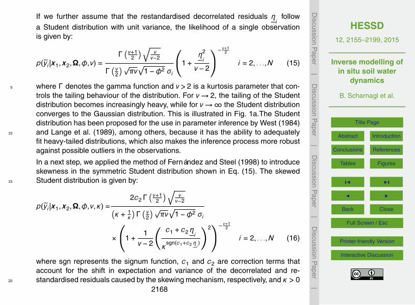
If we further assume that the restandardised decorrelated residuals ηi
follow
a Student distribution with unit variance, the likelihood of a single observationis given by:
p(yi |x1,x2,Ω,φ,ν) =Γ( ν+1
2
)√ νν−2
Γ( ν
2
)√πν√
1−φ2 σi
1+η2
i
ν−2
−ν+1
2
i = 2, . . .,N (15)
where Γ denotes the gamma function and ν>2 is a kurtosis parameter that con-5
trols the tailing behaviour of the distribution. For ν→ 2, the tailing of the Studentdistribution becomes increasingly heavy, while for ν→∞ the Student distributionconverges to the Gaussian distribution. This is illustrated in Fig. 1a.The Studentdistribution has been proposed for the use in parameter inference by West (1984)and Lange et al. (1989), among others, because it has the ability to adequately10
fit heavy-tailed distributions, which also makes the inference process more robustagainst possible outliers in the observations.
In a next step, we applied the method of Fernández and Steel (1998) to introduceskewness in the symmetric Student distribution shown in Eq. (15). The skewedStudent distribution is given by:15
p(yi |x1,x2,Ω,φ,ν,κ) =2c2Γ
( ν+12
)√ νν−2(
κ + 1κ
)Γ( ν
2
)√πν√
1−φ2 σi
×
1+1
ν−2
( c1 +c2ηi
κsgn(c1+c2 ηi)
)2−
ν+12
i = 2, . . .,N (16)
where sgn represents the signum function, c1 and c2 are correction terms thataccount for the shift in expectation and variance of the decorrelated and re-standardised residuals caused by the skewing mechanism, respectively, and κ > 020
2168
HESSD12, 2155–2199, 2015
Inverse modelling ofin situ soil water
dynamics
B. Scharnagl et al.
Title Page
Abstract Introduction
Conclusions References
Tables Figures
J I
J I
Back Close
Full Screen / Esc
Printer-friendly Version
Interactive Discussion
Discussion
Paper
|D
iscussionP
aper|
Discussion
Paper
|D
iscussionP
aper|
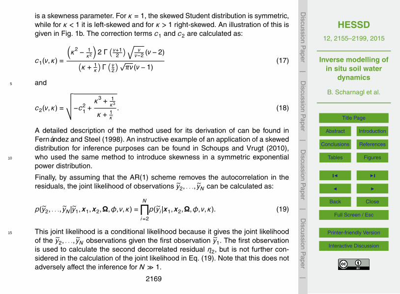
is a skewness parameter. For κ = 1, the skewed Student distribution is symmetric,while for κ < 1 it is left-skewed and for κ > 1 right-skewed. An illustration of this isgiven in Fig. 1b. The correction terms c1 and c2 are calculated as:
c1(ν,κ) =
(κ2 − 1
κ2
)2 Γ( ν+1
2
)√ νν−2 (ν−2)(
κ + 1κ
)Γ( ν
2
)√πν (ν−1)
(17)
and5
c2(ν,κ) =
√√√√−c21 +
κ3 + 1κ3
κ + 1κ
. (18)
A detailed description of the method used for its derivation of can be found inFernández and Steel (1998). An instructive example of an application of a skeweddistribution for inference purposes can be found in Schoups and Vrugt (2010),who used the same method to introduce skewness in a symmetric exponential10
power distribution.
Finally, by assuming that the AR(1) scheme removes the autocorrelation in theresiduals, the joint likelihood of observations y2, . . ., yN can be calculated as:
p(y2, . . ., yN |y1,x1,x2,Ω,φ,ν,κ) =N∏i=2
p(yi |x1,x2,Ω,φ,ν,κ). (19)
This joint likelihood is a conditional likelihood because it gives the joint likelihood15
of the y2, . . ., yN observations given the first observation y1. The first observationis used to calculate the second decorrelated residual η2, but is not further con-sidered in the calculation of the joint likelihood in Eq. (19). Note that this does notadversely affect the inference for N 1.
2169

HESSD12, 2155–2199, 2015
Inverse modelling ofin situ soil water
dynamics
B. Scharnagl et al.
Title Page
Abstract Introduction
Conclusions References
Tables Figures
J I
J I
Back Close
Full Screen / Esc
Printer-friendly Version
Interactive Discussion
Discussion
Paper
|D
iscussionP
aper|
Discussion
Paper
|D
iscussionP
aper|
Likelihood 3: The third likelihood model differs from the previous likelihood model inthat it implements a modified AR(1) scheme that does not suffer from the defi-ciency of the classical scheme used in the previous likelihood model. The modi-fied AR(1) scheme is given by:
ηi (x,x2,Ω,φ) = εi −φεi−1+φN
N∑j=1
εj i = 2, . . .,N (20)5
where the last term on the right hand side assures that the expectation of ηiwill always be the same as the expectation of εi . This can be seen from takingexpectations of both sides of Eq. (20):
E(ηi ) = E(εi )−E(φ)E(εi−1)+E(φ)E(εi )
= E(εi ) i = 2, . . .,N (21)10
where again we used E(εi ) = E(εi−1). All other assumptions are the same as
for Likelihood 2, we solely replace Eq. (13) by the modified expression givenin Eq. (20). We show in this study that the use of the modified AR(1) schemeremoves the bias in the model prediction caused by the classic AR(1) scheme.Furthermore, statistical inference using Likelihood 3 resulted in reliable parame-15
ter estimates that fulfilled the underlying assumptions of the likelihood model.
As mentioned in Sect. 2.1, the time series of soil water content observations hasa gap of about five days. The gap does not affect the calculations in the ordinary least-squares scheme of Likelihood 1. However, it calls for an extra step when using Likeli-hoods 2 and 3. This is because the autoregressive schemes applied in these likelihood20
models requires the same distance between neighbouring observations. For these twomodels, we therefore calculated two joint likelihoods, one for the first part of the timeseries of observations, and another one for the second part after the data gap. Thesetwo likelihoods were then multiplied to compute the likelihood to observe the entire dataset.25
2170

HESSD12, 2155–2199, 2015
Inverse modelling ofin situ soil water
dynamics
B. Scharnagl et al.
Title Page
Abstract Introduction
Conclusions References
Tables Figures
J I
J I
Back Close
Full Screen / Esc
Printer-friendly Version
Interactive Discussion
Discussion
Paper
|D
iscussionP
aper|
Discussion
Paper
|D
iscussionP
aper|
2.4 Bayes’ theorem
The joint likelihood summarizes in a probabilistic way what we can learn about the esti-mated parameters given the observations. However, sometimes it is desirable to makeexplicit use of prior knowledge about the parameters in the inference process. Bayes’theorem provides a formal way of combining information from observations with prior5
information about the estimated parameters. In case of Likelihood 1, Bayes’ theoremcan be written as:
p(x1,x2,σconst|y) ∝ p(x1) p(x2)p(σconst) p(y|x1,x2,σconst) (22)
where the term p(x1,x2,σconst|y) on the left hand side is the posterior density of theestimated parameters given the observations. p(x1), p(x2), and p(σconst) represent the10
prior densities of the parameters, and p(y|x1,x2,σconst) is just Likelihood 1, given inEq. (10). Similar expressions for the posterior density are obtained for Likelihood 2and 3.
For computational reasons, it is often not the prior, likelihood, and posterior that isused in practice, but rather its natural logarithm. This is because the prior, likelihood,15
and posterior may take on values larger or smaller than the largest or smallest numberthat can be represented by a double-precision floating-point format. This is especiallytrue if the joint likelihood of a large number of observations is calculated, as it was thecase in the present study. The log-prior, log-likelihood, and log-posterior was there-fore used in all calculations, and it is these numbers that are reported here as model20
diagnostics.
2.5 Prior densities
In order to apply Bayes’ theorem, the prior densities of the parameters need to bedefined. As a prior of the VGM parameters we chose a truncated multivariate normaldistribution p(x1) ∼ T N (µx1
,Σx1,ax1
,bx1), where µx denotes the mean vector of the25
VGM parameters, Σx is the corresponding covariance matrix, and ax1and bx1
represent2171

HESSD12, 2155–2199, 2015
Inverse modelling ofin situ soil water
dynamics
B. Scharnagl et al.
Title Page
Abstract Introduction
Conclusions References
Tables Figures
J I
J I
Back Close
Full Screen / Esc
Printer-friendly Version
Interactive Discussion
Discussion
Paper
|D
iscussionP
aper|
Discussion
Paper
|D
iscussionP
aper|
the upper and lower bounds, respectively. The mean vector and covariance matrix wasderived in Scharnagl et al. (2011) using the ROSETTA pedotransfer function (Schaapet al., 2001). Here, we make use of the full covariance matrix (Prior 3 in Scharnagl et al.,2011), which also contains information about the correlation structure of x1. In addition,we used the lower and upper bounds on the VGM parameters reported in Scharnagl5
et al. (2011) and listed in Table 1 to truncate the Gaussian distribution. The use of thetruncated multivariate normal distribution resulted in slightly faster convergence of theMarkov chains (Sect. 2.6) to the region of the parameter space with highest posteriordensity compared to using the conventional multivariate normal distribution as a prior.
The priors of the remaining parameters were given by a uniform distribution, which10
assigns a constant probability density within a specified interval and zero else. Thisso-called noninformative prior reflects our knowledge about these parameters beforethe inference process. In case of the pressure head at the lower boundary, the uniformprior can formally be written as p(x2) ∼ U(ax2
,bx2), where ax2
and bx2denote the cor-
responding lower and upper bound of that parameter, respectively. Similar expressions15
can be given for the unknown parameters in the likelihood model. The boundaries forall these parameters are also listed in Table 1.
We used a log10-transformation for parameters α, n, and Ks in the VGM model(Scharnagl et al., 2011). The kurtosis parameter in Likelihood 2 and 3 was transformedto 1/ν following the suggestion of Lange et al. (1989). These transformations aim at20
reducing nonlinear correlations of the estimated parameters, which helps to improvethe performance of the MCMC scheme.
2.6 Markov chain Monte Carlo simulation
The posterior distribution in Eq. (22) cannot be calculated by analytical means. Instead,we used MCMC simulation (e.g. Brooks, 1998) to generate samples from the poste-25
rior distribution. We used the Differential-Evolution-Markov-chain (DE-MC) framework(ter Braak, 2006; ter Braak and Vrugt, 2008) to run the MCMC simulations. The algo-rithm we applied generates candidate points from an archive of past states (DE-MC(Z),
2172

HESSD12, 2155–2199, 2015
Inverse modelling ofin situ soil water
dynamics
B. Scharnagl et al.
Title Page
Abstract Introduction
Conclusions References
Tables Figures
J I
J I
Back Close
Full Screen / Esc
Printer-friendly Version
Interactive Discussion
Discussion
Paper
|D
iscussionP
aper|
Discussion
Paper
|D
iscussionP
aper|
ter Braak and Vrugt, 2008) and decides upon their acceptance by the Metropolis ruleMetropolis et al. (1953). We did two minor changes to the standard DE-MC(Z) scheme,which aimed at improving the performance of this MCMC scheme. Without these mod-ifications, the exploration of the parameter space by the various Markov chains runin parallel was quite poor if Likelihood 2 or 3 was used. In fact, standard DE-MC(Z)5
even failed to locate the region of the parameter space with highest posterior density insome of the test runs. The two modifications improved the performance in these casessubstantially. The two modifications are as follows:
1. We implemented a block updating scheme, similar to what was used in ter Braak(2006). The idea behind block updating is that the convergence to a stationary10
distribution can sometimes be increased substantially if only a subset of the es-timated parameters is updated in a single step. This general finding motivatedVrugt et al. (2009a) to implement a self-adaptive randomized updating schemeinto DE-MC, resulting in the DiffeRential Evolution Adaptive Metropolis (DREAM)algorithm. This updating strategy did not work well in our application, presumably15
because it ignores the correlation structure of the VGM parameters induced bythe informative prior of these parameters. Instead of the randomized subspacesampling used in DREAM, we therefore used a block updating scheme, as fol-lows. For the first 2000 steps in each of the parallel chains, each parameter blockwas updated with probability 0.8. The VGM parameters were considered a block,20
whereas the remaining parameters were considered a block each. This simpleblock updating scheme increased the exploration capabilities of the Markov chainsand the convergence to a stationary distribution substantially. The block updatingwas restricted to the initial phase of the MCMC simulation because it is not par-ticularly efficient any more once the chains have approached to the stationary25
distribution.
2. Roberts and Rosenthal (2001) suggested that acceptance rates between 0.15and 0.5 can generally be considered efficient, with an optimal value being 0.23.
2173

HESSD12, 2155–2199, 2015
Inverse modelling ofin situ soil water
dynamics
B. Scharnagl et al.
Title Page
Abstract Introduction
Conclusions References
Tables Figures
J I
J I
Back Close
Full Screen / Esc
Printer-friendly Version
Interactive Discussion
Discussion
Paper
|D
iscussionP
aper|
Discussion
Paper
|D
iscussionP
aper|
Within standard DE-MC, the jumping distance of a proposal is scaled such thatoptimal acceptance rates are obtained when sampling from Gaussian and Stu-dent posteriors (Roberts and Rosenthal, 2001; ter Braak, 2006). Here, we intro-duce a factor r (dimensionless) that reduces this reference scaling of the jumpingdistance. The reasoning for this reduction is that efficient sampling from poste-5
rior distributions that differ from the multivariate Gaussian or Student distributiongenerally require smaller jumps than those taken by the reference scaling used inthe standard DE-MC scheme. In the present study, the reduction factor was set tor = 1.0 in the case of Likelihood 1, that is, no reduction, and r = 0.5 in the cases ofLikelihood 2 and 3. With these settings, acceptance rates near the optimal value10
of 0.23 were obtained in all three cases.
Apart from these two changes to the DE-MC(Z) scheme, we used standard settingsfor the algorithmic parameters reported by ter Braak (2006) and ran five chains inparallel. Convergence of the Markov chains to the stationary distribution was monitoredusing the interval diagnostic of Brooks and Gelman (1998). After convergence, we ran15
each of the five chains for another 10 000 steps. Parameter inference was based on5000 samples selected from this final sampling stage by thinning the chains, that is,by retaining every 10th sample. The calculation of the uncertainty bounds of the modelprediction is described in Schoups and Vrugt (2010), and is therefore not repeatedherein.20
3 Results
Figure 2 shows the results of inverse modelling of the time series of in situ soil watercontent observations using Likelihood 1 together with precipitation and potential evapo-ration fluxes that define the upper boundary condition in HYDRUS-1-D. The parameterestimates that belong to the prediction with maximum posterior density are listed in25
Table 1. This table also lists the corresponding mean error, root mean square error,
2174

HESSD12, 2155–2199, 2015
Inverse modelling ofin situ soil water
dynamics
B. Scharnagl et al.
Title Page
Abstract Introduction
Conclusions References
Tables Figures
J I
J I
Back Close
Full Screen / Esc
Printer-friendly Version
Interactive Discussion
Discussion
Paper
|D
iscussionP
aper|
Discussion
Paper
|D
iscussionP
aper|
model efficiency (Nash and Sutcliffe, 1970), as well as the log-prior, log-likelihood, andlog-posterior, which serve as model diagnostics to rate the goodness of the modelprediction. Based on visual inspection of Fig. 2, the ordinary least-squares approachimplemented in the first likelihood model results in a good overall description of the ob-servational data. This impression is also corroborated by the various model diagnostics5
listed in Table 2.To check the assumptions of homoscedastic, independent, and Gaussian distributed
standardised residuals εi used in ordinary least-squares, we made use of three diag-nostic plots. Figure 3a depicts the standardised residuals plotted against the simulatedsoil water content. This diagnostic plot indicates that the residuals are heteroscedastic.10
The SD of the residuals increases with increasing values of the predicted soil watercontent. Figure 3b shows the autocorrelation function of the residuals. This diagnosticplot shows that the residuals are strongly autocorrelated. The autocorrelation of theresiduals at lag 1, representing a time interval of 3 h, is close to one. The autocor-relation decreases rather slowly with increasing lag in an approximately exponential15
manner, which points to an autoregressive process of first order (e.g. Box et al., 2008).At lag 60, corresponding to a temporal separation of 7.5 days, the autocorrelation isstill significant, as indicated by the theoretical 95 % uncertainty bounds for a time se-ries of uncorrelated random variables. Figure 3c depicts a quantile–quantile plot ofthe standardised residuals. This diagnostic plot indicates that the actual distribution20
of the standardised residuals differs from that of a Gaussian distribution. The actualdistribution appears to be bimodal and also differs in its tailing behaviour from that ofa Gaussian distribution. In summary, the three diagnostic plots show that neither of thethree assumptions used in the formulation of Likelihood 1 is fulfilled. In this case, goodstatistical practice requires that the likelihood model is revised and that the inference25
process is repeated with the revised likelihood function.The results for Likelihood 2, which allows for heteroscedastic, autocorrelated, and
non-Gaussian distributed residuals, are presented in Fig. 4. The predicted soil watercontent deviates substantially and consistently from the observations. Clearly, the pa-
2175
HESSD12, 2155–2199, 2015
Inverse modelling ofin situ soil water
dynamics
B. Scharnagl et al.
Title Page
Abstract Introduction
Conclusions References
Tables Figures
J I
J I
Back Close
Full Screen / Esc
Printer-friendly Version
Interactive Discussion
Discussion
Paper
|D
iscussionP
aper|
Discussion
Paper
|D
iscussionP
aper|
rameter estimates obtained with this likelihood model are rather meaningless. They vi-olate the fundamental assumption of zero expectation of the residuals given in Eq. (7).Essentially the same results were obtained by Wöhling and Vrugt (2011), who alsoused the classical AR(1) scheme in their case study. We explain this repeated failurewith the fact that the classical AR(1) scheme introduces bias in the expected value5
of the residuals, as shown in Eq. (13). Figure 4 shows that the decorrelated and re-standardised residuals η
iare on average very close to zero even though the standard-
ised residuals εi deviate substantially from this value. This is reflected by a large meanerror and root mean square error of the prediction listed in Table 2. As briefly discussedin Sect. 2.3, the bias of the classical AR(1) scheme increases with increasing values10
of the autocorrelation coefficient φ. Indeed, the estimated autocorrelation coefficient φobtained with Likelihood 2 is very close to the upper bound of this parameter (Table 1).For φ→ 1, the AR(1) process becomes instationary, which is clearly not a meaningfulresult in a parameter inference setting.
In contrast, the modified AR(1) scheme used in Likelihood 3 does not suffer from the15
deficiency of the classical scheme, as shown in Eq. (21). The results obtained with thislikelihood model are depicted in Fig. 5. The prediction gives a good overall descriptionof the observations, which by visual inspection appears to be as good as the predictionobtained with Likelihood 1. Using the modified AR(1) scheme implemented in Likeli-hood 3, both the standardised residuals εi and the decorrelated and restandardised20
residuals εi have an expectation close to zero and a SD close to one. This result isobtained with an estimated autocorrelation coefficient φ that does not touch the up-per bound of this parameter and has a significant smaller value then that obtainedwith Likelihood 2 (Table 1). The mean error and root mean square error of the modelpredicted soil water content are slightly larger for Likelihood 3 compared to values ob-25
tained with Likelihood 1 (Table 2), while the model efficiency indicates an equally goodperformance of both models. From a statistical point of view, however, the superiority ofthe parameter estimates obtained with Likelihood 3 over the ones obtained with Like-lihood 1 becomes evident when comparing the corresponding posterior densities. The
2176

HESSD12, 2155–2199, 2015
Inverse modelling ofin situ soil water
dynamics
B. Scharnagl et al.
Title Page
Abstract Introduction
Conclusions References
Tables Figures
J I
J I
Back Close
Full Screen / Esc
Printer-friendly Version
Interactive Discussion
Discussion
Paper
|D
iscussionP
aper|
Discussion
Paper
|D
iscussionP
aper|
log-likelihood as well as the log-posterior obtained with Likelihood 3 are substantiallylarger than the corresponding values obtained with Likelihood 1 (Table 2). The largerlog-likelihood value already indicates that Likelihood 3 better describes the statisticalfeatures of the residuals.
Figure 6 illustrates the standardization of the residuals using the PCHIP approach5
and also shows the diagnostic plots used to check the underlying assumptions of thelikelihood model. In Fig. 6a, the raw residuals εi are plotted as a function of the pre-dicted soil water content. It becomes visible here that the variance of the raw resid-uals varies as function of the predicted soil water content, that is, that the εi are het-eroscedastic. However, what becomes also clear from this figure is that the expectation10
of the raw residuals also varies as a function of the predicted soil water content. Thesoil hydrological model systematically overestimates larger observations, which is anobvious expression of bias of the process model. The results of the PCHIP approach toestimate the SD of the raw residuals as a function of the predicted soil water content isshown in Fig. 6b. The corresponding standardised residuals εi are depicted in Fig. 6c.15
The standardised residuals appear to be homoscedastic, even though the systematicdeviation of the expectation of εi persists. We explain this by the fact that the PCHIPapproach partially compensates for model bias by assigning larger SDs to the morebiased residuals.
The three assumptions of homoscedasticity, independence, and skewed Student dis-20
tribution of the decorrelated and restandardised residuals ηi
that underlie Likelihood 3
are checked in the three diagnostic plots shown in Fig. 6d to f. These plots show thatthe three underlying assumptions are approximately fulfilled in the case of Likelihood 3.The decorrelated and restandardised residuals η
iused in this likelihood model appear
to be approximately homoscedastic, independent, and skewed Student distributed.25
From a statistical point of view, the parameter estimates obtained with Likelihood 3can therefore be considered statistically valid. It is also noteworthy that the estimatedvalues of the kurtosis parameter ν and the skewness parameter κ indicate that theactual distribution of the residuals deviates substantially from that of a Gaussian dis-
2177

HESSD12, 2155–2199, 2015
Inverse modelling ofin situ soil water
dynamics
B. Scharnagl et al.
Title Page
Abstract Introduction
Conclusions References
Tables Figures
J I
J I
Back Close
Full Screen / Esc
Printer-friendly Version
Interactive Discussion
Discussion
Paper
|D
iscussionP
aper|
Discussion
Paper
|D
iscussionP
aper|
tribution. The parameter estimates given in Table 1 show that the actual distribution ismuch more heavy tailed than the Gaussian distribution and that it is slightly left-skewed.
In the following, we compare the estimated soil hydrological parameters and theresulting soil hydraulic functions obtained with Likelihood 1 and 3. Figure 7 depictspairwise scatter plots of the posterior samples obtained with these two likelihood mod-5
els together with the prior 95 % uncertainty regions. The figure illustrates that all modelparameter were identified uniquely. Although some of the soil hydrological parameterscorrelated strongly, all parameter estimates generally showed little variance. Anotherimportant result of this comparison was that the parameter estimates obtained withLikelihood 1 and 3 differ systematically. The pairwise scatter plots show almost no10
overlap of the two posterior samples. It is noteworthy that the shape of the posteriorsample obtained with Likelihood 3 deviates somewhat from that of a multivariate normaldistribution. Even this slight deviation, however, adversely affected the performance ofthe MCMC scheme and gave reason for the use of a reduced reference scaling of thejumping distance described in Sect. 2.6. The uniqueness of the estimated parame-15
ters was not restricted to the hydrological parameters, but was also observed for theparameters of the likelihood model. The posterior samples for these parameters gener-ally showed little variance and no strong correlations with any of the other parameters,neither with those of the likelihood model nor with those of the soil hydrological model(not shown).20
The soil hydraulic properties computed from the posterior samples obtained withLikelihood 1 and 3 are depicted in Fig. 8. In this figure, we display the 95 % poste-rior uncertainty bounds for the water retention and hydraulic conductivity function to-gether with the corresponding 95 % prior uncertainty bounds. The posterior uncertaintybounds are generally very tight, reflecting the high precision of the soil hydraulic pa-25
rameters which is illustrated in Fig. 7. In general, the posterior uncertainty bounds aretightest in the intermediate soil water content range, which corresponds to the range ofactual soil water content observations. This is also where the soil hydraulic functionsobtained with the two likelihood models match each other most.
2178
HESSD12, 2155–2199, 2015
Inverse modelling ofin situ soil water
dynamics
B. Scharnagl et al.
Title Page
Abstract Introduction
Conclusions References
Tables Figures
J I
J I
Back Close
Full Screen / Esc
Printer-friendly Version
Interactive Discussion
Discussion
Paper
|D
iscussionP
aper|
Discussion
Paper
|D
iscussionP
aper|
4 Discussion
The application of Likelihood 1, which makes use of the ordinary least-squares as-sumptions, resulted in parameter estimates that are invalid from a statistical point ofview because the residuals violate all underlying assumptions of this likelihood model.Neglecting autocorrelation in the residuals means to overestimate the information con-5
tent of the data and therefore leads to an underestimation of parameter uncertainty.This becomes evident in the parameter sample from the posterior shown in Fig. 7:the variance of the posterior obtained with Likelihood 1 is generally smaller than thatobtained with Likelihood 3. If residuals are correlated, the amount of information pro-vided by each observation is smaller than in the case of uncorrelated observations. In10
fact, using a likelihood model which neglects autocorrelation essentially implies to treatthe soil hydrological model as if it was perfect. This is overoptimistic because environ-mental models are – almost by definition – at best good approximations of real-worldprocesses: they cannot be perfect.
We showed that the classical AR(1) scheme implemented in Likelihood 2 resulted15
in unrealistic parameter estimates and, correspondingly, to biased model predictions.This corroborates the results reported by Wöhling and Vrugt (2011), who used theclassical AR(1) scheme in a soil hydrological application. We showed analytically thatthe AR(1) scheme introduces bias, which explains the failure of this autoregressivemodel in the present study as well as in the application of Wöhling and Vrugt (2011).20
Obviously, inverse modelling of in situ soil water dynamics seems to be much more sus-ceptible to the bias problem induced by the classical AR(1) scheme than, for example,inverse problems in catchment hydrology, where it has been applied successfully manytimes (e.g. Sorooshian and Dracup, 1980; Bates and Campbell, 2001). We conjecturethat this is because the systematic misfit between observations and model predictions25
depicted in Fig. 4 can easily be compensated for by an estimated value of the au-tocorrelation coefficient that is larger than actually necessary. In a recent study, Evinet al. (2014) showed that the results obtained with the classical AR(1) model applied
2179

HESSD12, 2155–2199, 2015
Inverse modelling ofin situ soil water
dynamics
B. Scharnagl et al.
Title Page
Abstract Introduction
Conclusions References
Tables Figures
J I
J I
Back Close
Full Screen / Esc
Printer-friendly Version
Interactive Discussion
Discussion
Paper
|D
iscussionP
aper|
Discussion
Paper
|D
iscussionP
aper|
to inverse modelling of stream flow can be nonrobust, indicated by strong correlationsbetween parameters in the hydrological model and the likelihood model. We suspectthat the reason for this nonrobustness might also be explained, at least partially, withthe bias that is introduced by the classical AR(1) scheme.
The residuals obtained with Likelihood 3 clearly satisfied all assumptions of this likeli-5
hood model and furthermore demonstrate that Likelihood 3 solves the bias-problem in-herent to Likelihood 2. Since the log-likelihood and log-posterior values for Likelihood 3were substantially larger than those obtained with Likelihood 1 (Table 2), we considerthis likelihood function and the parameter estimates obtained with it as clearly superiorand statistically valid. The model predictions obtained with Likelihood 3 slightly vio-10
late the zero-expectation assumption, which becomes apparent from the non-constantexpectation of the residuals shown in Fig. 6a. This model bias can in principle be ac-counted for in the formulation of the likelihood model by introducing a term for biascorrection, which can for example be estimated as a function of the predicted soil wa-ter content (e.g. Kennedy and O’Hagan, 2001; Erdal et al., 2012). From our point of15
view, however, such an approach would not be meaningful in the present application.This is because the bias correction would be valid only for the depth within the soilprofile where the observations were taken, but it remains unclear how this bias cor-rection affects the predicted soil water contents at other depths within the profile andthe fluxes to adjacent compartments within the water cycle. This is a fundamental dif-20
ference between the Bayesian approach adopted in this study and other statisticalapproaches that are designed to account for model bias, such as particle filtering (e.g.Montzka et al., 2011; Vrugt et al., 2013). Within the the present statistical framework,we think that the model bias can therefore only be meaningfully corrected for by a thor-ough revision of the process model, the assumption of a homogeneous profile, the25
parametrisation of the soil hydraulic properties, and the inclusion of hysteresis.Likelihood 3, which allows for heteroscedastic, autocorrelated, and non-Gaussian
residuals, may be equally useful in other soil hydrological applications. In general, au-tocorrelation of the residuals becomes increasingly apparent if observations are taken
2180

HESSD12, 2155–2199, 2015
Inverse modelling ofin situ soil water
dynamics
B. Scharnagl et al.
Title Page
Abstract Introduction
Conclusions References
Tables Figures
J I
J I
Back Close
Full Screen / Esc
Printer-friendly Version
Interactive Discussion
Discussion
Paper
|D
iscussionP
aper|
Discussion
Paper
|D
iscussionP
aper|
at a sufficiently high temporal frequency, which is typically the case for automated mea-surement setups either in the field or in the laboratory. For example, autocorrelation ofthe residuals is particularly pronounced in inverse modelling of multi-step outflow ex-periments (e.g. Diamantopoulos et al., 2012), evaporation experiments (e.g. Dettmannet al., 2014), or lysimeter data (e.g. Schelle et al., 2012). Based on the findings of the5
present study, we conjecture that a likelihood model that allows for heteroscedastic,autocorrelated, and non-Gaussian residuals would also prove useful in these applica-tions. The main advantages are a more accurate quantification of the model parametersand their uncertainty. In the case of multiple time series used for parameter inference,Likelihood 3 must be extended to the multivariate case by using a first-order vector10
autoregressive (VAR(1)) model (e.g. Box et al., 2008). In contrast to the AR(1) modeltreated in this study, the VAR(1) model additionally accounts for the cross-correlationbetween the multiple, parallel time series of observations.
5 Summary and conclusions
In this case study, we estimated the soil hydraulic properties of a homogeneous, bare15
soil profile from in situ observations of soil water content taken at a single location nearthe soil surface. This type of observational data often contain too little information towarrant accurate and precise estimates of all of the parameters in the soil hydrologicalmodel. We posed the inverse problem in a formal Bayesian approach, which allowedus to use prior information of the soil hydraulic parameters in terms of an informative20
prior distribution for these parameters. The prior distribution was taken from Scharnaglet al. (2011). We then applied three likelihood models, which differ in their underlyingassumptions about the salient statistical features of the time series of residuals.
The first likelihood model corresponds to the ordinary least-squares approach, whichis the de facto standard in inverse modelling of soil hydrological processes. However,25
the results obtained with Likelihood 1 showed that the underlying assumptions of thislikelihood model of homoscedastic, independent, and Gaussian residuals were all vio-
2181

HESSD12, 2155–2199, 2015
Inverse modelling ofin situ soil water
dynamics
B. Scharnagl et al.
Title Page
Abstract Introduction
Conclusions References
Tables Figures
J I
J I
Back Close
Full Screen / Esc
Printer-friendly Version
Interactive Discussion
Discussion
Paper
|D
iscussionP
aper|
Discussion
Paper
|D
iscussionP
aper|
lated. From a statistical point of view, the parameter estimates obtained with this firstlikelihood model can therefore be considered invalid.
The second likelihood model makes use of the classical AR(1) scheme to accountfor autocorrelated residuals, allows for heteroscedasticity, and supports heavily-tailed,non-Gaussian distributions of the residuals. To describe the heteroscedastic nature of5
the residuals, we devised a flexible model for the relationship between model predictedsoil water content and the SD of the residuals that uses cubic Hermite interpolation. De-viations from a Gaussian distribution were modelled with a skewed Student distribution.A theoretical analysis of this parameter inference scheme and the results obtained withLikelihood 2 demonstrated that the classical AR(1) model introduces bias into the infer-10
ence process. Due to this bias, the results obtained with Likelihood 2 were essentiallymeaningless, which corroborates the findings of Wöhling and Vrugt (2011) obtained ina similar soil hydrological study and using the same classical AR(1) scheme.
In the third likelihood model, we introduced a modified AR(1) scheme, which doesnot suffer from the bias problem induced by the classical scheme. With this likelihood15
model, we obtained parameter estimates that differed significantly from those obtainedwith Likelihood 1, which implements the ordinary least-squares assumptions. Further-more, parameter uncertainty was higher as compared to Likelihood 1 because thedecreased information content of the calibration data caused by autocorrelation wasaccounted for. Since the residuals obtained with Likelihood 3 fulfilled the underlying sta-20
tistical assumptions, and because Likelihood 3 lead to a much larger log-posterior thanLikelihood 1, we concluded that the parameter estimates obtained with Likelihood 3 arestatistically valid, and therefore, superior to the ones obtained with Likelihood 1.
The results of this study demonstrate that the ordinary least-squares approach maylead to statistically invalid estimates of the soil hydraulic parameters, because the un-25
derlying assumptions about the statistical features of the time series of residuals arenot fulfilled. The current practice in inverse modelling of soil hydrological processesshould therefore be revised. We introduced a new, highly flexible likelihood model thataccounts for autocorrelated, heteroscedastic, and non-Gaussian residuals, which per-
2182

HESSD12, 2155–2199, 2015
Inverse modelling ofin situ soil water
dynamics
B. Scharnagl et al.
Title Page
Abstract Introduction
Conclusions References
Tables Figures
J I
J I
Back Close
Full Screen / Esc
Printer-friendly Version
Interactive Discussion
Discussion
Paper
|D
iscussionP
aper|
Discussion
Paper
|D
iscussionP
aper|
formed very well in the present test study. Based on our findings, we advocate the useand further extension of the new likelihood model in inverse modelling of soil hydrolog-ical processes.
Acknowledgements. We thank Marius Schmidt and Karl Schneider for providing the meteo-rological data used to define the upper boundary conditions. We also acknowledge the help5
of Nils Prolingheuer during the measurement setup and data collection. The first, fourth,and fifth author gratefully acknowledge financial support by the TERENO project and bySFB/TR 32 “Patterns in Soil–Vegetation–Atmosphere Systems: Monitoring, Modelling, andData Assimilation” funded by the Deutsche Forschungsgemeinschaft (DFG).
10
The service charges for this open-access publicationhave been covered by a Research Centre of theHelmholtz Association.
References
Allen, R. G., Pereira, L. S., Raes, D. S., and Smith, M.: Crop evapotranspiration (guidelines for15
computing crop water requirements), no. 56, in: FAO Irrigation and Drainage Paper No. 56,Food and Agricultural Organization of the United Nations, Rome, Italy, 1998. 2162
Baroni, G., Facchi, A., Gandolfi, C., Ortuani, B., Horeschi, D., and van Dam, J. C.: Uncer-tainty in the determination of soil hydraulic parameters and its influence on the performanceof two hydrological models of different complexity, Hydrol. Earth Syst. Sci., 14, 251–270,20
doi:10.5194/hess-14-251-2010, 2010. 2157Basile, A., Ciollaro, G., and Coppola, A.: Hysteresis in soil water characteristics as a key to in-
terpreting comparisons of laboratory and field measured hydraulic properties, Water Resour.Res., 39, 1355, doi:10.1029/2003WR002432, 2003. 2157
Bates, B. C. and Campbell, E. P.: A Markov chain Monte Carlo scheme for parameter estima-25
tion and inference in conceptual rainfall-runoff modeling, Water Resour. Res., 37, 937–947,doi:10.1029/2000WR900363, 2001. 2167, 2179
Beach, C. M. and MacKinnon, J. G.: A maximum likelihood procedure for regression with auto-correlated errors, Econometrica, 46, 51–58, 1978. 2159
2183

HESSD12, 2155–2199, 2015
Inverse modelling ofin situ soil water
dynamics
B. Scharnagl et al.
Title Page
Abstract Introduction
Conclusions References
Tables Figures
J I
J I
Back Close
Full Screen / Esc
Printer-friendly Version
Interactive Discussion
Discussion
Paper
|D
iscussionP
aper|
Discussion
Paper
|D
iscussionP
aper|
Bitterlich, S., Durner, W., Iden, S. C., and Knabner, P.: Inverse estimation of the unsaturatedsoil hydraulic properties from column outflow experiments using free-form parameterizations,Vadose Zone J., 3, 971–981, doi:10.2136/vzj2004.0971, 2004. 2166
Box, G. E. P., Jenkins, G. M., and Reinsel, G. C.: Time Series Analyis: Forcasting and Control,3rd Edn., John Wiley and Sons, Hoboken, NJ, USA, 2008. 2166, 2167, 2175, 21815
Brooks, S. P.: Markov chain Monte Carlo method and its application, J. Roy. Stat. Soc. D-Stat.,47, 69–100, doi:10.1111/1467-9884.00117, 1998. 2172
Brooks, S. P. and Gelman, A.: General methods for monitoring convergence of iterative simu-lations, J. Comput. Graph. Stat., 7, 434–455, doi:10.1080/10618600.1998.10474787, 1998.217410
Carsel, R. F. and Parrish, R. S.: Developing joint probability distributions of soil water retentioncharacteristics, Water Resour. Res., 24, 755–769, doi:10.1029/WR024i005p00755, 1988.2159
Cochrane, D. and Orcutt, G. H.: Application of least squares regression to rela-tionships containing auto-correlated error terms, J. Am. Stat. Assoc., 44, 32–61,15
doi:10.1080/01621459.1949.10483290, 1949. 2159Dane, J. H. and Wierenga, P. J.: Effect of hysteresis on the prediction of infiltration, redistri-
bution and drainage of water in a layered soil, J. Hydrol., 25, 229–242, doi:10.1016/0022-1694(75)90023-2, 1975. 2157
Dettmann, U., Bechtold, M., Frahm, E., and Tiemeyer, B.: On the applicability of unimodal20
and bimodal van Genuchten–Mualem based models to peat and other organic soils underevaporation conditions, J. Hydrol., 515, 103–115, doi:10.1016/j.jhydrol.2014.04.047, 2014.2181
Diamantopoulos, E. and Durner, W.: Dynamic nonequilibrium of water flow in porous media: areview, Vadose Zone J., 11, doi:10.2136/vzj2011.0197, 2012. 215725
Diamantopoulos, E., Iden, S. C., and Durner, W.: Inverse modeling of dynamic non-equilibrium in water flow with an effective approach, Water Resour. Res., 48, W03503,doi:10.1029/2011WR010717, 2012. 2181
Doherty, J. and Welter, D.: A short exploration of structural noise, Water Resour. Res., 46,W05525, doi:10.1029/2009WR008377, 2010. 215930
Durner, W. and Iden, S. C.: Extended multistep outflow method for the accurate determina-tion of soil hydraulic properties near water saturation, Water Resour. Res., 47, W08526,doi:10.1029/2011WR010632, 2011. 2157
2184

HESSD12, 2155–2199, 2015
Inverse modelling ofin situ soil water
dynamics
B. Scharnagl et al.
Title Page
Abstract Introduction
Conclusions References
Tables Figures
J I
J I
Back Close
Full Screen / Esc
Printer-friendly Version
Interactive Discussion
Discussion
Paper
|D
iscussionP
aper|
Discussion
Paper
|D
iscussionP
aper|
Erdal, D., Neuweiler, I., and Huisman, J. A.: Estimating effective model parameters for hetero-geneous unsaturated flow using error models for bias correction, Water Resour. Res., 48,W06530, doi:10.1029/2011WR011062, 2012. 2180
Evin, G., Kavetski, D., Thyer, M., and Kuczera, G.: Pitfalls and improvements in the joint in-ference of heteroscedasticity and autocorrelation in hydrological model calibration, Water5
Resour. Res., 49, 4518–4524, doi:10.1002/wrcr.20284, 2013. 2166Evin, G., Thyer, M., Kavetski, D., McInerney, D., and Kuczera, G.: Comparison of joint
versus postprocessor approaches for hydrological uncertainty estimation accountingfor error autocorrelation and heteroscedasticity, Water Resour. Res., 50, 2350–2375,doi:10.1002/2013WR014185, 2014. 217910
Fernández, C. and Steel, M. F. J.: On Bayesian modeling of fat tails and skewness, J. Am. Stat.Assoc., 93, 359–371, doi:10.1080/01621459.1998.10474117, 1998. 2168, 2169
Fritsch, F. N. and Carlson, R. E.: Monotone piecewise cubic interpolation, SIAM J. Numer. Anal.,17, 238–246, doi:10.1137/0717021, 1980. 2165
Heimovaara, T. J. and Bouten, W.: A computer-controlled 36-channel time domain reflec-15
tometry system for monitoring soil water contents, Water Resour. Res., 26, 2311–2316,doi:10.1029/WR026i010p02311, 1990. 2161
Hou, Z. and Rubin, Y.: On minimum relative entropy concepts and prior compatibility is-sues in vadose zone inverse and forward modeling, Water Resour. Res., 41, W12425,doi:10.1029/2005WR004082, 2005. 215820
Iden, S. C. and Durner, W.: Free-form estimation of the unsaturated soil hydraulic prop-erties by inverse modeling using global optimization, Water Resour. Res., 43, W07451,doi:10.1029/2006WR005845, 2007. 2166
IUSS Working Group WRB: World Reference Base for Soil Resources 2006, World Soil Re-sources Reports No. 103, first updated Edn., Food and Agricultural Organization of the25
United Nations, Rome, Italy, 2007. 2161Jacques, D., Šimůnek, J., Timmerman, A., and Feyen, J.: Calibration of Richards’ and
convection-dispersion equations to field-scale water flow and solute transport under rainfallconditions, J. Hydrol., 259, 15–31, doi:10.1016/S0022-1694(01)00591-1, 2002. 2165
Kavetski, D., Kuczera, G., and Franks, S. W.: Bayesian analysis of input uncertainty in hydro-30
logical modeling: 1. Theory, Water Resour. Res., 42, W03407, doi:10.1029/2005WR004368,2006. 2164
2185

HESSD12, 2155–2199, 2015
Inverse modelling ofin situ soil water
dynamics
B. Scharnagl et al.
Title Page
Abstract Introduction
Conclusions References
Tables Figures
J I
J I
Back Close
Full Screen / Esc
Printer-friendly Version
Interactive Discussion
Discussion
Paper
|D
iscussionP
aper|
Discussion
Paper
|D
iscussionP
aper|
Kennedy, M. C. and O’Hagan, A.: Bayesian calibration of computer models, J. Roy. Stat. Soc.B, 63, 425–464, doi:10.1111/1467-9868.00294, 2001. 2180
Kuczera, G.: Improved parameter inference in catchment models: 1. Evaluating parameter un-certainty, Water Resour. Res., 19, 1151–1162, doi:10.1029/WR019i005p01151, 1983. 2159,21675
Lange, K. L., Little, R. J. A., and Taylor, J. M. G.: Robust statistical modeling using the t distribu-tion, J. Am. Stat. Assoc., 84, 881–896, doi:10.1080/01621459.1989.10478852, 1989. 2168,2172
Lenhard, R. J., Parker, J. C., and Kaluarachchi, J. J.: Comparing simulated and experimentalhysteretic two-phase transient fluid flow phenomena, Water Resour. Res., 27, 2113–2124,10
doi:10.1029/91WR01272, 1991. 2157Mallants, D., Mohanty, B. P., Vervoort, A., and Feyen, J.: Spatial analysis of saturated hydraulic
conductivity in a soil with macropores, Soil Technol., 10, 115–131, doi:10.1016/S0933-3630(96)00093-1, 1997. 2157
Mertens, J., Madsen, H., Kristensen, M., Jacques, D., and Feyen, J.: Sensitivity of soil parame-15
ters in unsaturated zone modelling and the relation between effective, laboratory and in situestimates, Hydrol. Process., 19, 1611–1633, doi:10.1002/hyp.5591, 2005. 2157
Metropolis, N., Rosenbluth, A. W., Rosenbluth, M. N., Teller, A. H., and Teller, E.: Equa-tion of state calculations by fast computing machines, J. Chem. Phys., 21, 1087–1091,doi:10.1063/1.1699114, 1953. 217320
Montzka, C., Moradkhani, H., Weihermüller, L., Hendricks Franssen, H.-J., Canty, M., andVereecken, H.: Hydraulic parameter estimation by remotely-sensed top soil moisture obser-vations with the particle filter, J. Hydrol., 399, 410–421, doi:10.1016/j.jhydrol.2011.01.020,2011. 2180
Nash, J. E. and Sutcliffe, J. V.: River flow forecasting through conceptual models part I A discus-25
sion of principles, J. Hydrol., 10, 282–290, doi:10.1016/0022-1694(70)90255-6, 1970. 2175Peters, A. and Durner, W.: Simplified evaporation method for determining soil hydraulic proper-
ties, J. Hydrol., 356, 147–162, doi:10.1016/j.jhydrol.2008.04.016, 2008. 2157Roberts, G. O. and Rosenthal, J. S.: Optimal scaling for various Metropolis-Hastings algorithms,
Stat. Sci., 16, 351–367, doi:10.1214/ss/1015346320, 2001. 2173, 217430
Schaap, M. G., Leij, F. J., and van Genuchten, M. T.: ROSETTA: a computer program for es-timating soil hydraulic parameters with hierarchical pedotransfer functions, J. Hydrol., 251,163–176, doi:10.1016/S0022-1694(01)00466-8, 2001. 2158, 2172
2186

HESSD12, 2155–2199, 2015
Inverse modelling ofin situ soil water
dynamics
B. Scharnagl et al.
Title Page
Abstract Introduction
Conclusions References
Tables Figures
J I
J I
Back Close
Full Screen / Esc
Printer-friendly Version
Interactive Discussion
Discussion
Paper
|D
iscussionP
aper|
Discussion
Paper
|D
iscussionP
aper|
Scharnagl, B., Vrugt, J. A., Vereecken, H., and Herbst, M.: Inverse modelling of in situ soilwater dynamics: investigating the effect of different prior distributions of the soil hydraulicparameters, Hydrol. Earth Syst. Sci., 15, 3043–3059, doi:10.5194/hess-15-3043-2011, 2011.2158, 2159, 2160, 2161, 2163, 2164, 2172, 2181
Schelle, H., Iden, S. C., Fank, J., and Durner, W.: Inverse estimation of soil hydraulic and root5
distribution parameters from lysimeter data, Vadose Zone J., 11, doi:10.2136/vzj2011.0169,2012. 2165, 2181
Scholer, M., Irving, J., Binley, A., and Holliger, K.: Estimating vadose zone hydraulic propertiesusing ground penetrating radar: the impact of prior information, Water Resour. Res., 47,W10512, doi:10.1029/2011WR010409, 2011. 2158, 215910
Schoups, G. and Vrugt, J. A.: A formal likelihood function for parameter and predictive infer-ence of hydrologic models with correlated, heteroscedastic, and non-Gaussian errors, WaterResour. Res., 46, W10531, doi:10.1029/2009WR008933, 2010. 2169, 2174
Sonnleitner, M. A., Abbaspour, K. C., and Schulin, R.: Hydraulic and transport propertiesof the plant-soil system estimated by inverse modelling, Eur. J. Soil Sci., 54, 127–138,15
doi:10.1046/j.1365-2389.2002.00491.x, 2003. 2165Sorooshian, S. and Dracup, J. A.: Stochastic parameter estimation procedures for hydraulic
rainfall-runoff models: correlated and heteroscedastic error cases, Water Resour. Res., 16,430–442, doi:10.1029/WR016i002p00430, 1980. 2159, 2167, 2179
ter Braak, C. J. F.: A Markov chain Monte Carlo version of the genetic algorithm Differential20
Evolution: easy Bayesian computing for real parameter spaces, Stat. Comput., 16, 239–249,doi:10.1007/s11222-006-8769-1, 2006. 2172, 2173, 2174
ter Braak, C. J. F. and Vrugt, J. A.: Differential evolution Markov chain with snooker updater andfewer chains, Stat. Comput., 18, 435–446, doi:10.1007/s11222-008-9104-9, 2008. 2172,217325
Topp, G. C., Davis, J. L., and Annan, A. P.: Electromagnetic determination of soil watercontent: Measurements in coaxial transmission lines, Water Resour. Res., 16, 574–582,doi:10.1029/WR016i003p00574, 1980. 2161
van Dam, J. C., Stricker, J. N. M., and Droogers, P.: Inverse method to determine soil hy-draulic functions from multistep outflow experiments, Soil Sci. Soc. Am. J., 58, 647–652,30
doi:10.2136/sssaj1994.03615995005800030002x, 1994. 2157
2187

HESSD12, 2155–2199, 2015
Inverse modelling ofin situ soil water
dynamics
B. Scharnagl et al.
Title Page
Abstract Introduction
Conclusions References
Tables Figures
J I
J I
Back Close
Full Screen / Esc
Printer-friendly Version
Interactive Discussion
Discussion
Paper
|D
iscussionP
aper|
Discussion
Paper
|D
iscussionP
aper|
van Genuchten, M. T.: A closed-form equation for predicting the hydraulicconductivity of unsaturated soils, Soil Sci. Soc. Am. J., 44, 892–898,doi:10.2136/sssaj1980.03615995004400050002x, 1980. 2162
Vereecken, H., Huisman, J. A., Bogena, H., Vanderborght, J., Vrugt, J. A., and Hopmans, J. W.:On the value of soil moisture measurements in vadose zone hydrology: a review, Water5
Resour. Res., 44, W00D06, doi:10.1029/2008WR006829, 2008. 2158Vrugt, J. A., Braak, C. J. F., Diks, C. G. H., Robinson, B. A., Hyman, J. M., and Higdon, D.:
Accelerating Markov chain Monte Carlo simulation by differential evolution with self-adaptiverandomized subspace sampling, Int. J. Nonlin. Sci. Num., 10, 271–288, 2009a. 2173
Vrugt, J. A., Braak, C. J. F., Gupta, H. V., and Robinson, B. A.: Equifinality of formal (DREAM)10
and informal (GLUE) Bayesian approaches in hydrologic modeling?, Stoch. Env. Res. RiskA., 23, 1011–1026, doi:10.1007/s00477-008-0274-y, 2009b. 2167
Vrugt, J. A., ter Braak, C. J. F., Diks, C. G. H., and Schoups, G.: Hydrologic data assimilationusing particle Markov chain Monte Carlo simulation: theory, concepts and applications, Adv.Water Resour., 51, 457–478, doi:10.1016/j.advwatres.2012.04.002, 2013. 218015
Šimůnek, J., van Genuchten, M. T., and Wendroth, O.: Parameter estimation analysis of theevaporation method for determining soil hydraulic properties, Soil Sci. Soc. Am. J., 62, 894–905, doi:10.2136/sssaj1998.03615995006200040007x, 1998. 2157
Šimůnek, J., Šejna, M., Saito, H., Sakai, M., and van Genuchten, M. T.: The HYDRUS-1-D Soft-ware Package for Simulating the One-Dimensional Movement of Water, Heat and Multiple20
Solutes in Variably-Saturated Media (Version 4.0), Department of Environmental Sciences,University of California Riverside, Riverside, CA, USA, available at: http://www.pc-progress.com//Downloads/Pgm_Hydrus1D/HYDRUS1D_4.pdf (last access: 26 January 2015), 2008.2162
West, M.: Outlier models and prior distributions in Bayesian linear regression, J. Roy. Stat. Soc.25
B, 1, 431–439, 1984. 2168Wöhling, T. and Vrugt, J. A.: Multiresponse multilayer vadose zone model calibration using
Markov chain Monte Carlo simulation and field water retention data, Water Resour. Res., 47,W04510, doi:10.1029/2010WR009265, 2011. 2160, 2167, 2176, 2179, 2182
Wollschläger, U., Pfaff, T., and Roth, K.: Field-scale apparent hydraulic parameterisation ob-30
tained from TDR time series and inverse modelling, Hydrol. Earth Syst. Sci., 13, 1953–1966,doi:10.5194/hess-13-1953-2009, 2009. 2165
2188

HESSD12, 2155–2199, 2015
Inverse modelling ofin situ soil water
dynamics
B. Scharnagl et al.
Title Page
Abstract Introduction
Conclusions References
Tables Figures
J I
J I
Back Close
Full Screen / Esc
Printer-friendly Version
Interactive Discussion
Discussion
Paper
|D
iscussionP
aper|
Discussion
Paper
|D
iscussionP
aper|
Woodbury, A. D. and Ulrych, T. J.: Minimum relative entropy: forward probabilistic modeling,Water Resour. Res., 29, 2847–2860, doi:10.1029/93WR00923, 1993. 2158
2189

HESSD12, 2155–2199, 2015
Inverse modelling ofin situ soil water
dynamics
B. Scharnagl et al.
Title Page
Abstract Introduction
Conclusions References
Tables Figures
J I
J I
Back Close
Full Screen / Esc
Printer-friendly Version
Interactive Discussion
Discussion
Paper
|D
iscussionP
aper|
Discussion
Paper
|D
iscussionP
aper|
Table 1. Estimated parameters in the soil hydrological and likelihood model, respectively, aswell as parameter estimates with maximum posterior density obtained using the three differentlikelihood models.
parameter estimateswith maximum posterior density
lower upper likelihood likelihood likelihoodparameter unit transformation bound bound model 1 model 2 model 3
soil θr cm3 cm−3 – 0.043 0.091 0.051 0.061 0.053hydrological θs cm3 cm−3 – 0.409 0.481 0.461 0.460 0.436model α cm−1 log10(α) 0.0028 0.0085 0.0045 0.0051 0.0037
n – log10(n) 1.51 1.85 1.77 1.70 1.77Ks cm h−1 log10(Ks) 0.006 0.832 0.534 0.254 0.091L – – −5.49 6.27 4.20 1.76 3.67hLB cm – −250 −50 −170 −51 −178
likelihood σconst cm3 cm−3 – 0.000 0.025 0.0121model σa cm3 cm−3 – 0.000 0.050 0.0183 0.0092
σb cm3 cm−3 – 0.000 0.050 0.0190 0.0131σc cm3 cm−3 – 0.000 0.050 0.0316 0.0218σd cm3 cm−3 – 0.000 0.050 0.0498 0.0360φ – – 0.000 1.000 0.996 0.957ν – 1/ν 2.000 ∞ 3.32 2.89κ – – 0.500 2.000 1.27 0.85
2190

HESSD12, 2155–2199, 2015
Inverse modelling ofin situ soil water
dynamics
B. Scharnagl et al.
Title Page
Abstract Introduction
Conclusions References
Tables Figures
J I
J I
Back Close
Full Screen / Esc
Printer-friendly Version
Interactive Discussion
Discussion
Paper
|D
iscussionP
aper|
Discussion
Paper
|D
iscussionP
aper|
Table 2. Summary statistics of model residuals and the values of the prior, likelihood and pos-terior computed for the parameter estimates with maximum posterior density. Results are givenfor the three different likelihood models.
likelihood likelihood likelihoodmodel diagnostic model 1 model 2 model 3
mean error −0.0001 −0.0738 −0.0012root mean square error 0.0121 0.0754 0.0132model efficiency 0.74 0.01 0.74log-prior 23 28 27log-likelihood 3891 5880 5761log-posterior 3914 5908 5788
2191

HESSD12, 2155–2199, 2015
Inverse modelling ofin situ soil water
dynamics
B. Scharnagl et al.
Title Page
Abstract Introduction
Conclusions References
Tables Figures
J I
J I
Back Close
Full Screen / Esc
Printer-friendly Version
Interactive Discussion
Discussion
Paper
|D
iscussionP
aper|
Discussion
Paper
|D
iscussionP
aper|
0
0.2
0.4
0.6
0.8
prob
abili
tyde
nsity
κ = 1.0
ν = 20
ν = 5
ν = 2.5
Gaussian
a
−3 −2 −1 0 1 2 3standardized residuals
0
0.2
0.4
0.6
0.8
prob
abili
tyde
nsity
ν = 5
κ = 0.5
κ = 1.0
κ = 2.0
Gaussian
b
Figure 1. Illustration of the skewed Student distribution. In (a), the skewness parameter iskept constant (κ = 1) while the kurtosis parameter is varied. In (b), the skewness parameter isvaried while the kurtosis parameter is kept constant (ν = 5). To allow for a direct comparison,the corresponding Gaussian distribution is also shown. All distributions have an expectation ofzero and a SD of one.
2192

HESSD12, 2155–2199, 2015
Inverse modelling ofin situ soil water
dynamics
B. Scharnagl et al.
Title Page
Abstract Introduction
Conclusions References
Tables Figures
J I
J I
Back Close
Full Screen / Esc
Printer-friendly Version
Interactive Discussion
Discussion
Paper
|D
iscussionP
aper|
Discussion
Paper
|D
iscussionP
aper|
0.25
0.3
0.35
0.4
θ(c
m3
cm−
3)
a observed and predicted soil water content
−5
0
5
ε(−
)
b standardised residuals
120 140 160 180 200 220 240 260 280
day of year
-2
-1
0
1
P,E
pot
(cm
day−
1)
c potential evaporation
precipitation
Figure 2. Model prediction of the time series of soil water content observations obtained usingLikelihood 1. In (a), the model prediction with maximum posterior density and the 95 % uncer-tainty bounds of the prediction are shown together with the observations of soil water contentθ. (b) displays the standardised residuals ε
i, corresponding to the prediction with maximum
posterior density. (c) shows the precipitation P (negative) and potential evaporation Epot (pos-itive) fluxes used as input to the HYDRUS-1-D model. For graphical reasons, daily fluxes areshown here whereas hourly values were used to run the model.
2193
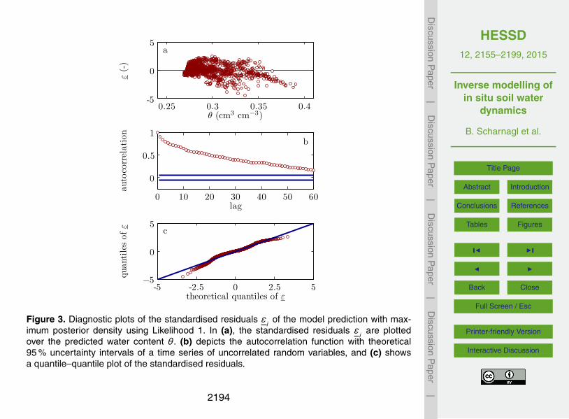
HESSD12, 2155–2199, 2015
Inverse modelling ofin situ soil water
dynamics
B. Scharnagl et al.
Title Page
Abstract Introduction
Conclusions References
Tables Figures
J I
J I
Back Close
Full Screen / Esc
Printer-friendly Version
Interactive Discussion
Discussion
Paper
|D
iscussionP
aper|
Discussion
Paper
|D
iscussionP
aper|
0.25 0.3 0.35 0.4θ (cm3 cm−3)
-5
0
5
ε(-
)
a
0 10 20 30 40 50 60lag
0
0.5
1au
toco
rrel
atio
n
b
theoretical quantiles of ε
quan
tile
sof
ε
-5 -2.5 0 2.5 5−5
0
5c
Figure 3. Diagnostic plots of the standardised residuals εi
of the model prediction with max-imum posterior density using Likelihood 1. In (a), the standardised residuals ε
iare plotted
over the predicted water content θ. (b) depicts the autocorrelation function with theoretical95 % uncertainty intervals of a time series of uncorrelated random variables, and (c) showsa quantile–quantile plot of the standardised residuals.
2194

HESSD12, 2155–2199, 2015
Inverse modelling ofin situ soil water
dynamics
B. Scharnagl et al.
Title Page
Abstract Introduction
Conclusions References
Tables Figures
J I
J I
Back Close
Full Screen / Esc
Printer-friendly Version
Interactive Discussion
Discussion
Paper
|D
iscussionP
aper|
Discussion
Paper
|D
iscussionP
aper|
0.25
0.3
0.35
0.4
0.45
θ(c
m3
cm−
3)
a observed and predicted soil water content
−5
0
5
ε(−
)
b standardised residuals
120 140 160 180 200 220 240 260 280
day of year
−20
0
20
η(−
)
c
decorrelated and restandardised residuals
Figure 4. Model prediction of the time series of soil water content observations obtained usingLikelihood 2. In (a), the model prediction with maximum posterior density and the 95 % uncer-tainty bounds of the prediction are shown together with the observations of soil water contentθ. (b) displays the standardised residuals ε
i, corresponding to the prediction with maximum
posterior density. (c) shows the decorrelated and restandardised residuals ηi.
2195

HESSD12, 2155–2199, 2015
Inverse modelling ofin situ soil water
dynamics
B. Scharnagl et al.
Title Page
Abstract Introduction
Conclusions References
Tables Figures
J I
J I
Back Close
Full Screen / Esc
Printer-friendly Version
Interactive Discussion
Discussion
Paper
|D
iscussionP
aper|
Discussion
Paper
|D
iscussionP
aper|
0.25
0.3
0.35
0.4
θ(c
m3
cm−
3)
a observed and predicted soil water content
−5
0
5
ε(−
)
b
standardised residuals
120 140 160 180 200 220 240 260 280
day of year
−20
0
20
η(−
)
c
decorrelated and restandardised residuals
Figure 5. Model prediction of the time series of soil water content observations obtained usingLikelihood 3. In (a), the model prediction with maximum posterior density and the 95 % uncer-tainty bounds of the prediction are shown together with the observations of soil water contentθ. (b) displays the standardised residuals ε
i, corresponding to the prediction with maximum
posterior density. (c) shows the decorrelated and restandardised residuals ηi.
2196

HESSD12, 2155–2199, 2015
Inverse modelling ofin situ soil water
dynamics
B. Scharnagl et al.
Title Page
Abstract Introduction
Conclusions References
Tables Figures
J I
J I
Back Close
Full Screen / Esc
Printer-friendly Version
Interactive Discussion
Discussion
Paper
|D
iscussionP
aper|
Discussion
Paper
|D
iscussionP
aper|
0.25 0.3 0.35 0.4θ (cm3 cm−3)
-0.06
0
0.06
ε(c
m3
cm−
3)
a
0.25 0.3 0.35 0.4θ (cm3 cm−3)
0
0.025
0.05
σ(c
m3
cm−
3)
b
0.25 0.3 0.35 0.4θ (cm3 cm−3)
-5
0
5
ε(−
)
c
0.25 0.3 0.35 0.4θ (cm3 cm−3)
-12
0
12
η(−
)
d
0 10 20 30 40 50 60lag
0
0.5
1
auto
corr
elat
ion
e
theoretical quantiles of η
quan
tile
sof
η-12 -6 0 6 12
-12
0
12f
Figure 6. Performance of the PCHIP approach used for standardization of the residuals anddiagnostic plots of the decorrelated and restandardised residuals corresponding to the modelprediction with maximum posterior density using Likelihood 3. (a) shows the residuals εi asa function of the predicted soil water content θ. (b) gives the estimated SD as a function ofthe predicted soil water content, showing the estimated points σa,...,d and the resulting functiongiven by the PCHIP. The grey area represents the corresponding 95 % uncertainty. In (c) thestandardised residuals ε
iare plotted over the predicted water content, while (d) shows the
decorrelated and restandardised residuals ηi. (e) depicts the autocorrelation function of η
iwith
theoretical 95 % uncertainty intervals of a time series of uncorrelated random variables, and(f) shows a quantile–quantile plot of η
i.
2197

HESSD12, 2155–2199, 2015
Inverse modelling ofin situ soil water
dynamics
B. Scharnagl et al.
Title Page
Abstract Introduction
Conclusions References
Tables Figures
J I
J I
Back Close
Full Screen / Esc
Printer-friendly Version
Interactive Discussion
Discussion
Paper
|D
iscussionP
aper|
Discussion
Paper
|D
iscussionP
aper|
θs
95 % prior uncertainty region
sample from posterior using Likelihood 1
sample from posterior using Likelihood 3log 1
0(α)
log 1
0(n
)log 1
0(K
s)L
θr
hLB
θs log10(α) log10(n) log10(K s) L
Figure 7. Pairwise scatter plots of the posterior samples of the parameters of the soil hydrolog-ical model obtained with Likelihood 1 and 3 together with the corresponding 95 % prior uncer-tainty regions of these parameters. The axes cover the parameter bounds listed in Table 1.
2198

HESSD12, 2155–2199, 2015
Inverse modelling ofin situ soil water
dynamics
B. Scharnagl et al.
Title Page
Abstract Introduction
Conclusions References
Tables Figures
J I
J I
Back Close
Full Screen / Esc
Printer-friendly Version
Interactive Discussion
Discussion
Paper
|D
iscussionP
aper|
Discussion
Paper
|D
iscussionP
aper|
0
0.1
0.2
0.3
0.4
0.5
θ(c
m3
cm−
3)
a Likelihood 1Likelihood 3
−104 −103 −102 −101 −100
h (cm)
10−10
10−8
10−6
10−4
10−2
100
K(c
mho
ur−
1)
b Likelihood 1
Likelihood 3
Prior
Figure 8. 95 % posterior uncertainty bounds of (a) the water retention function and (b) thehydraulic conductivity function obtained with Likelihood 1 and 3. Additionally, the corresponding95 % prior uncertainty regions are shown as a grey area.
2199


