
Ising Models for Neural Data John Hertz, Niels Bohr Institute and Nordita
work done with Yasser Roudi (Nordita) and Joanna Tyrcha (SU)
Math Bio Seminar, SU, 26 March 2009
arXiv:0902.2885v1 (2009)
Background and basic idea:
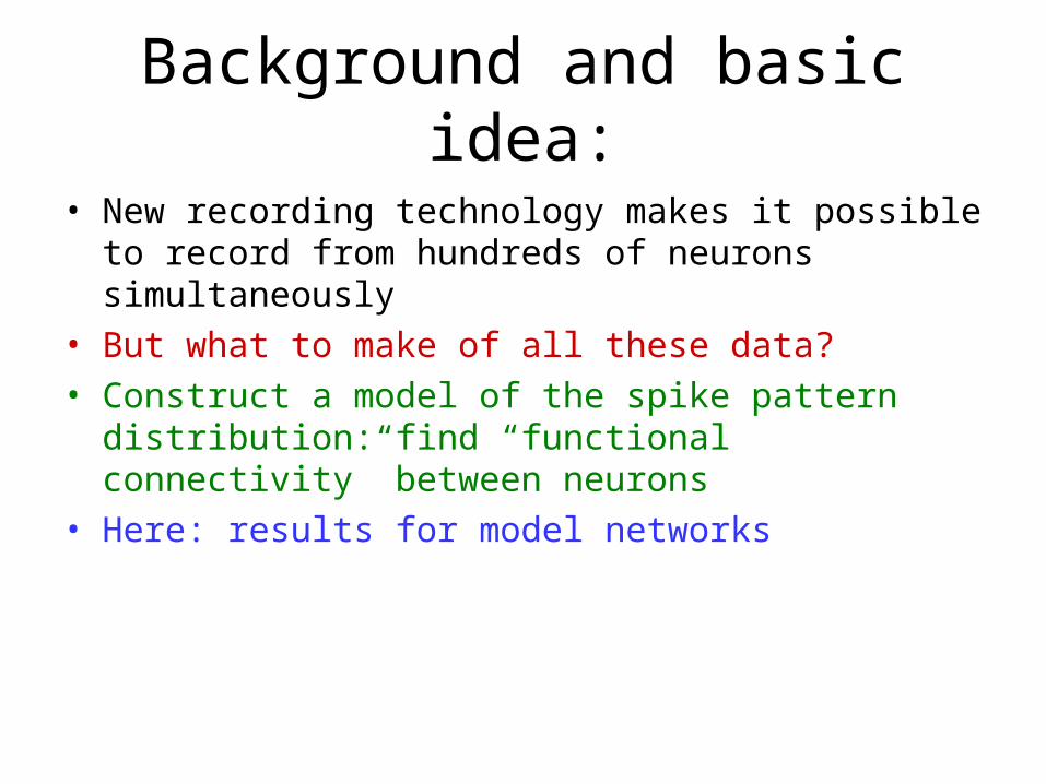
• New recording technology makes it possible to record from hundreds of neurons simultaneously
Background and basic idea:
• New recording technology makes it possible to record from hundreds of neurons simultaneously
• But what to make of all these data?
Background and basic idea:
• New recording technology makes it possible to record from hundreds of neurons simultaneously
• But what to make of all these data?• Construct a model of the spike pattern distribution: find
“functional connectivity” between neurons
Background and basic idea:
• New recording technology makes it possible to record from hundreds of neurons simultaneously
• But what to make of all these data?• Construct a model of the spike pattern distribution: find
“functional connectivity” between neurons• Here: results for model networks

Outline
Outline
• Data
Outline
• Data
• Model and methods, exact and approximate
Outline
• Data
• Model and methods, exact and approximate
• Results: accuracy of approximations, scaling of functional connections
Outline
• Data
• Model and methods, exact and approximate
• Results: accuracy of approximations, scaling of functional connections
• Quality of the fit to the data distribution
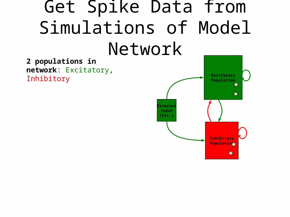
Get Spike Data from Simulations of Model Network2 populations in network: Excitatory, Inhibitory
ExcitatoryPopulation
InhibitoryPopulation
ExternalInput(Exc.)

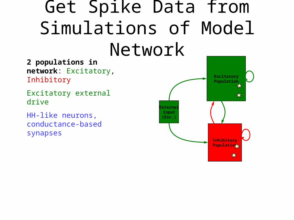
Get Spike Data from Simulations of Model Network2 populations in network: Excitatory, Inhibitory
Excitatory external drive
ExcitatoryPopulation
InhibitoryPopulation
ExternalInput(Exc.)
Get Spike Data from Simulations of Model Network2 populations in network: Excitatory, Inhibitory
Excitatory external drive
HH-like neurons, conductance-based synapses
ExcitatoryPopulation
InhibitoryPopulation
ExternalInput(Exc.)
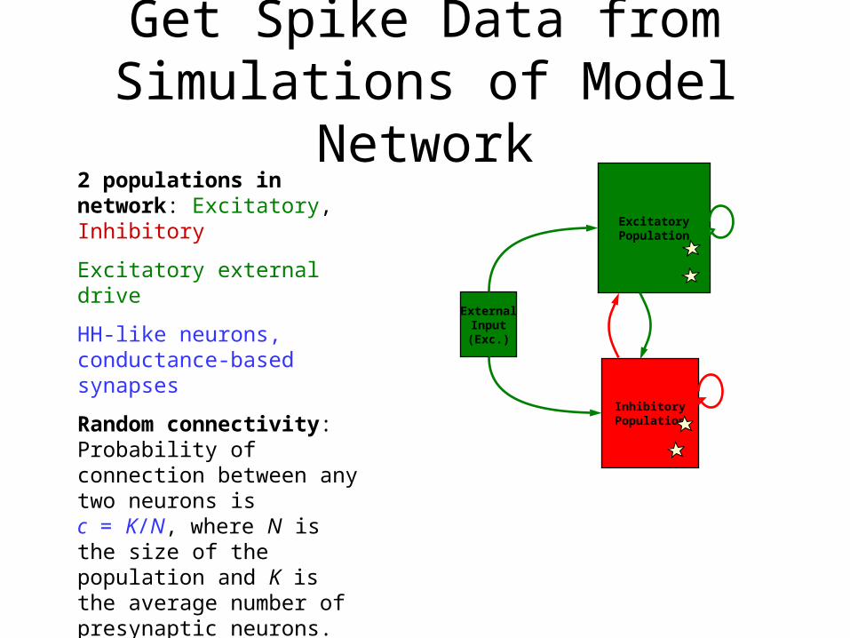
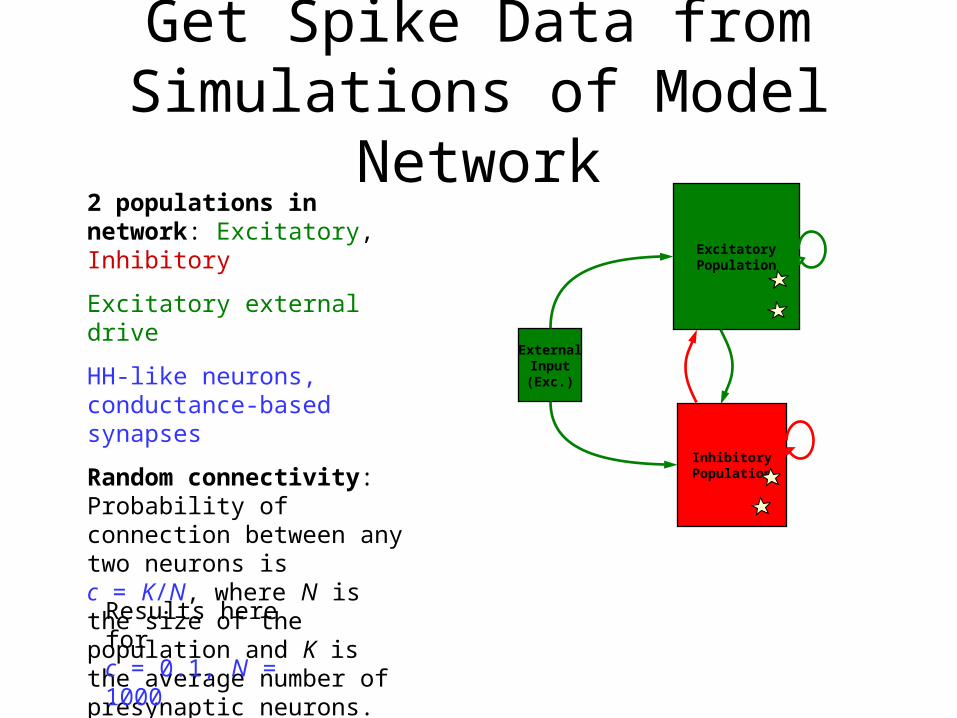
Get Spike Data from Simulations of Model Network2 populations in network: Excitatory, Inhibitory
Excitatory external drive
HH-like neurons, conductance-based synapses
Random connectivity:Probability of connection between any two neurons is c = K/N, where N is the size of the population and K is the average number of presynaptic neurons.
ExcitatoryPopulation
InhibitoryPopulation
ExternalInput(Exc.)
Results here for c = 0.1, N = 1000
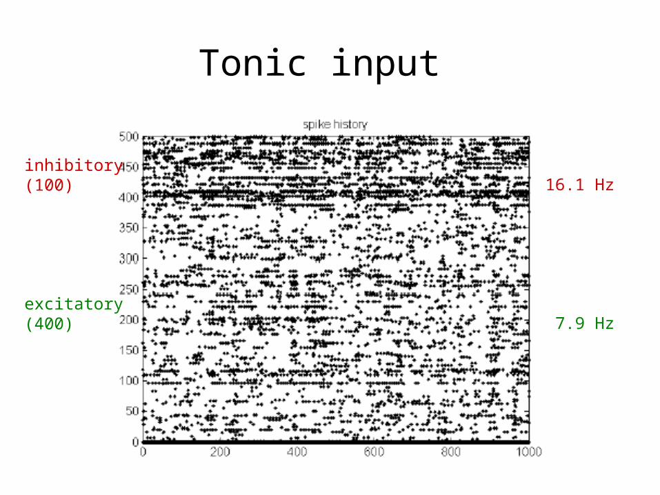
Tonic input
inhibitory(100)
excitatory(400)
16.1 Hz
7.9 Hz
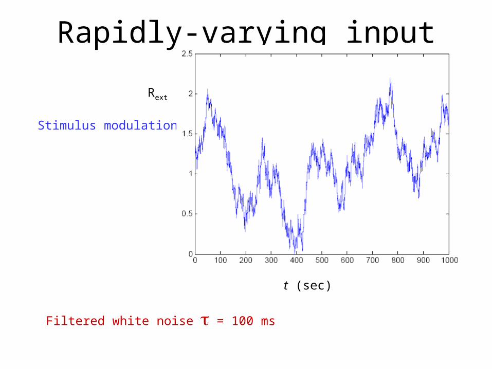
Rext
t (sec)
Filtered white noise = 100 ms
Stimulus modulation:
Rapidly-varying input
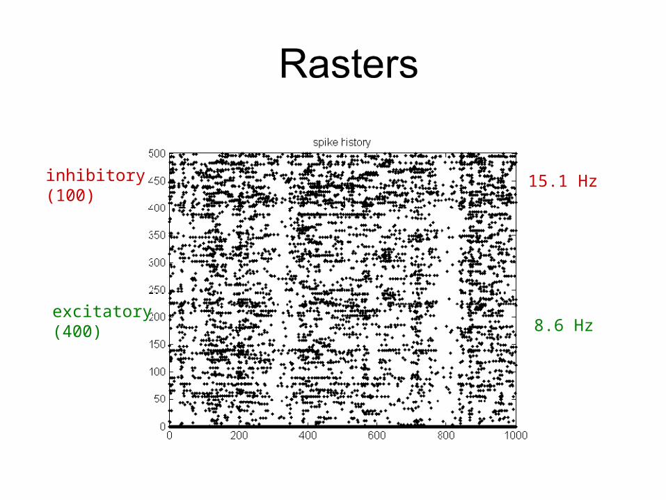
inhibitory(100)
excitatory(400)
15.1 Hz
8.6 Hz
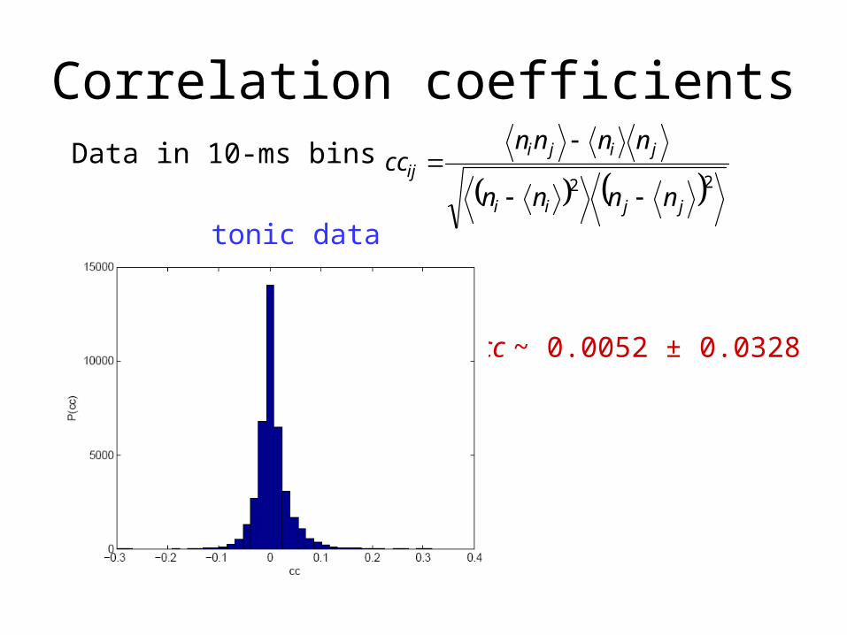
Correlation coefficientsData in 10-ms bins
22jjii
jijiij
nnnn
nnnncc
cc ~ 0.0052 ± 0.0328
tonic data
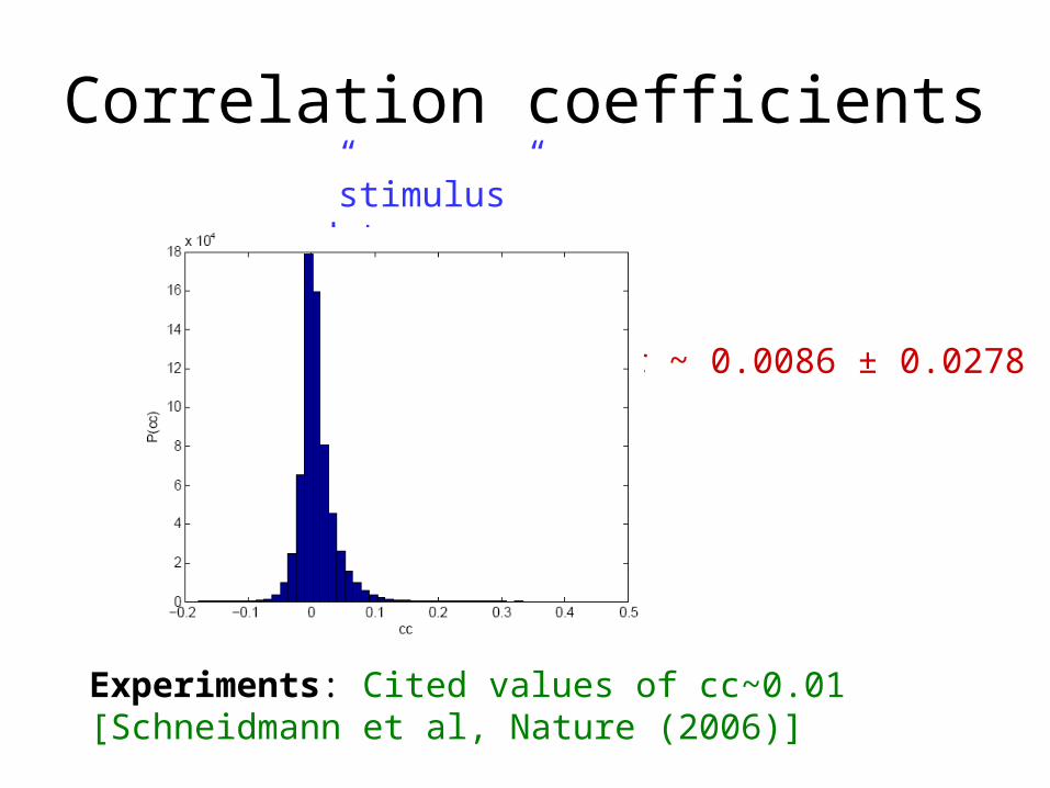
Correlation coefficients
cc ~ 0.0086 ± 0.0278
Experiments: Cited values of cc~0.01 [Schneidmann et al, Nature (2006)]
”stimulus” data
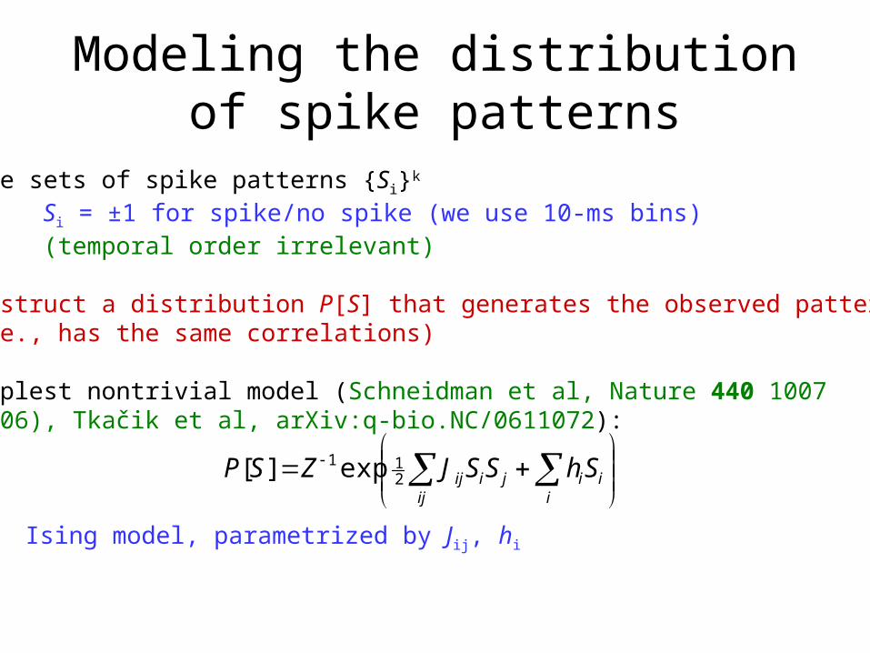
Modeling the distribution of spike patterns
Have sets of spike patterns {Si}k Si = ±1 for spike/no spike (we use 10-ms bins)(temporal order irrelevant)
Modeling the distribution of spike patterns
Have sets of spike patterns {Si}k Si = ±1 for spike/no spike (we use 10-ms bins)(temporal order irrelevant)
Construct a distribution P[S] that generates the observed patterns (i.e., has the same correlations)
Modeling the distribution of spike patterns
Have sets of spike patterns {Si}k Si = ±1 for spike/no spike (we use 10-ms bins)(temporal order irrelevant)
Construct a distribution P[S] that generates the observed patterns (i.e., has the same correlations)
Simplest nontrivial model (Schneidman et al, Nature 440 1007 (2006), Tkačik et al, arXiv:q-bio.NC/0611072):
ij iiijiij ShSSJZSP 2
11 exp][
Ising model, parametrized by Jij, hi
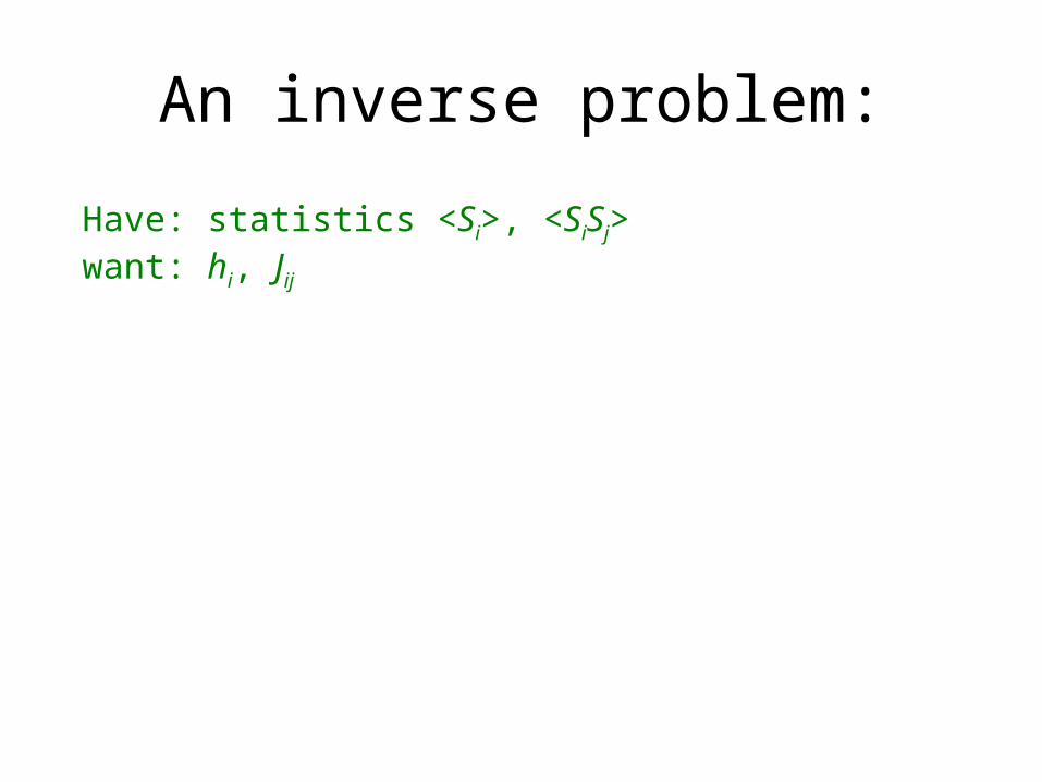
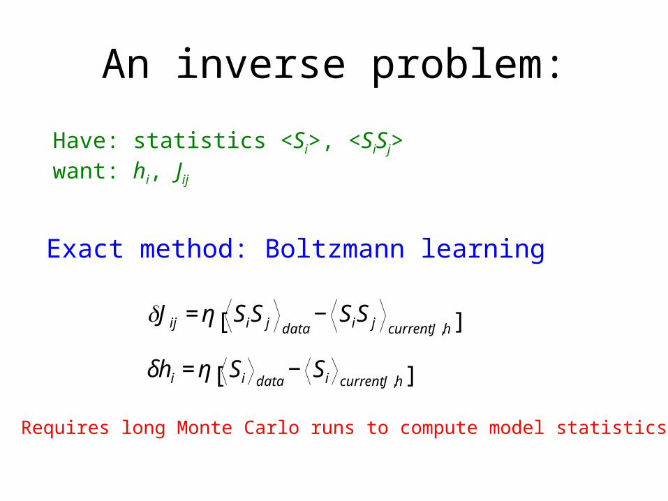
An inverse problem:
Have: statistics <Si>, <SiSj>want: hi, Jij
An inverse problem:
Have: statistics <Si>, <SiSj>want: hi, Jij
Exact method: Boltzmann learning
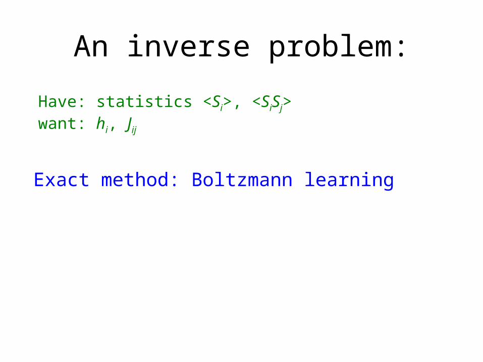
An inverse problem:
Have: statistics <Si>, <SiSj>want: hi, Jij
Exact method: Boltzmann learning
€
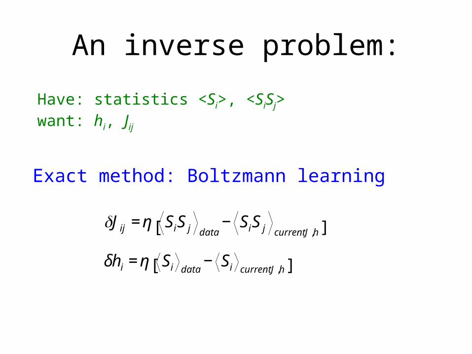
δJij = η SiS j data− SiS j current J ,h[ ]
δhi = η Si data− Si current J ,h[ ]
An inverse problem:
Have: statistics <Si>, <SiSj>want: hi, Jij
Exact method: Boltzmann learning
€
δJij = η SiS j data− SiS j current J ,h[ ]
δhi = η Si data− Si current J ,h[ ]
Requires long Monte Carlo runs to compute model statistics
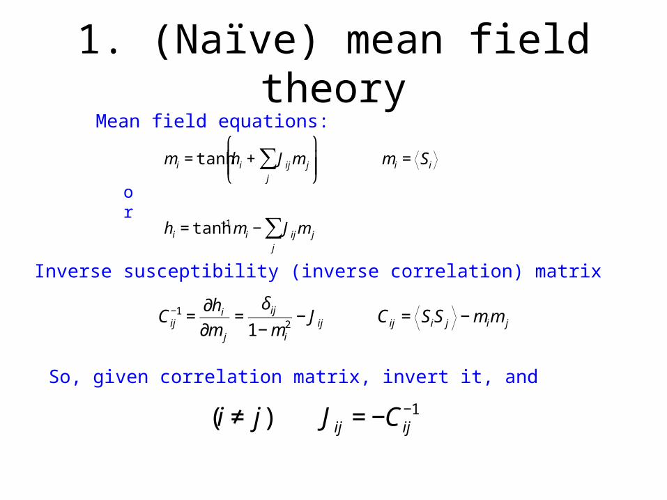
1. (Naïve) mean field theory
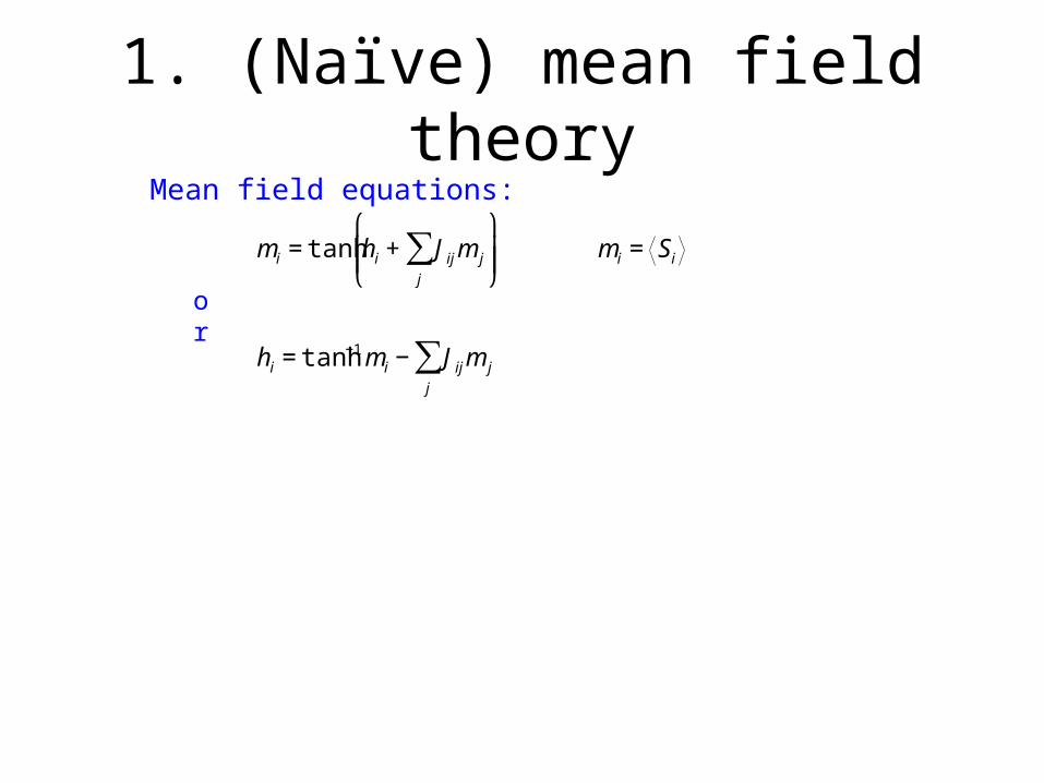
1. (Naïve) mean field theory
€
mi = tanh hi + Jijm j
j
∑ ⎛
⎝ ⎜ ⎜
⎞
⎠ ⎟ ⎟ mi = Si
hi = tanh−1 mi − Jijm j
j
∑
or
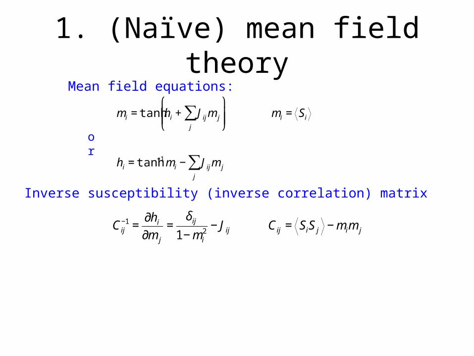
Mean field equations:
1. (Naïve) mean field theory
€
mi = tanh hi + Jijm j
j
∑ ⎛
⎝ ⎜ ⎜
⎞
⎠ ⎟ ⎟ mi = Si
hi = tanh−1 mi − Jijm j
j
∑
or
Inverse susceptibility (inverse correlation) matrix
€
Cij−1 =
∂hi
∂m j
=δ ij
1− mi2
− Jij Cij = SiS j − mim j
Mean field equations:
1. (Naïve) mean field theory
€
mi = tanh hi + Jijm j
j
∑ ⎛
⎝ ⎜ ⎜
⎞
⎠ ⎟ ⎟ mi = Si
hi = tanh−1 mi − Jijm j
j
∑
or
Inverse susceptibility (inverse correlation) matrix
€
Cij−1 =
∂hi
∂m j
=δ ij
1− mi2
− Jij Cij = SiS j − mim j
So, given correlation matrix, invert it, and
€
(i ≠ j) Jij = −Cij−1
Mean field equations:
2. TAP approximation
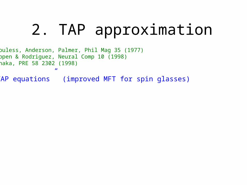
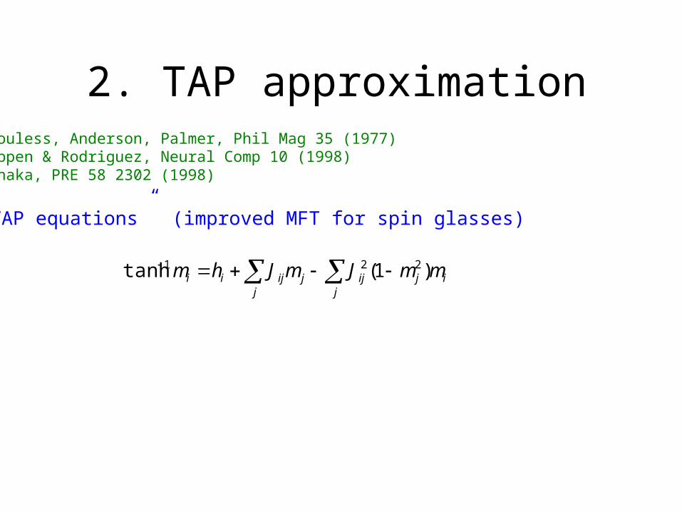
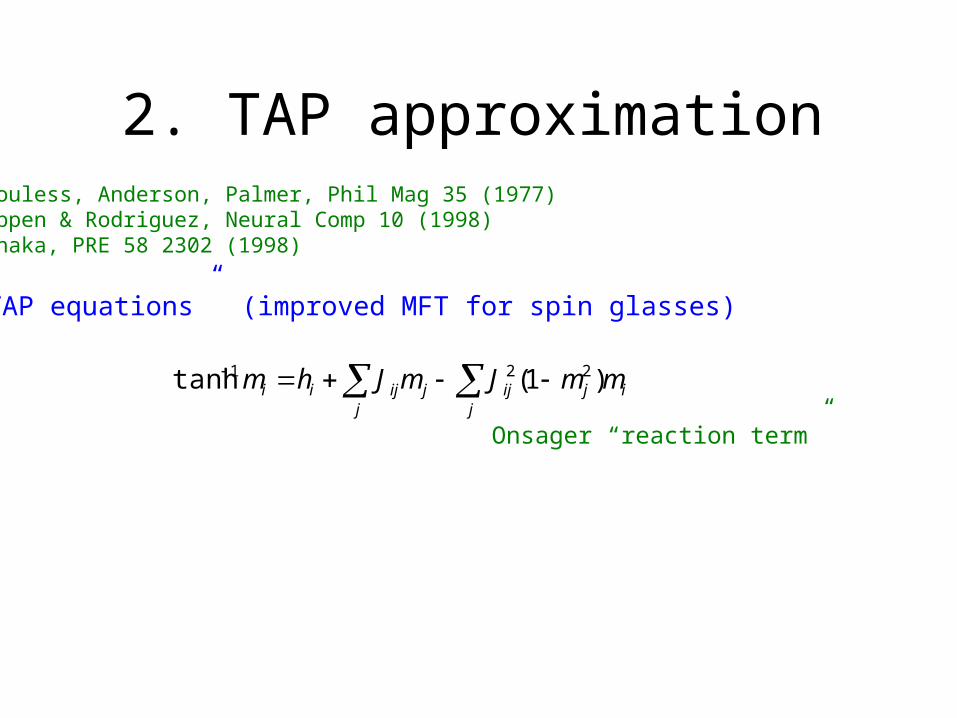
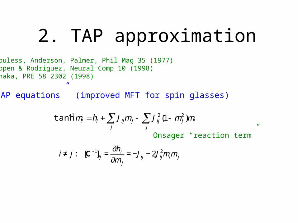
2. TAP approximationThouless, Anderson, Palmer, Phil Mag 35 (1977)Kappen & Rodriguez, Neural Comp 10 (1998)Tanaka, PRE 58 2302 (1998)
“TAP equations” (improved MFT for spin glasses)
2. TAP approximationThouless, Anderson, Palmer, Phil Mag 35 (1977)Kappen & Rodriguez, Neural Comp 10 (1998)Tanaka, PRE 58 2302 (1998)
“TAP equations” (improved MFT for spin glasses)
ijj
ijj
jijii mmJmJhm )1(tanh 221
2. TAP approximationThouless, Anderson, Palmer, Phil Mag 35 (1977)Kappen & Rodriguez, Neural Comp 10 (1998)Tanaka, PRE 58 2302 (1998)
“TAP equations” (improved MFT for spin glasses)
ijj
ijj
jijii mmJmJhm )1(tanh 221
Onsager “reaction term”
2. TAP approximationThouless, Anderson, Palmer, Phil Mag 35 (1977)Kappen & Rodriguez, Neural Comp 10 (1998)Tanaka, PRE 58 2302 (1998)
“TAP equations” (improved MFT for spin glasses)
ijj
ijj
jijii mmJmJhm )1(tanh 221
€
i ≠ j : [C-1]ij =∂hi
∂m j
= −Jij − 2Jij2mim j
Onsager “reaction term”

2. TAP approximationThouless, Anderson, Palmer, Phil Mag 35 (1977)Kappen & Rodriguez, Neural Comp 10 (1998)Tanaka, PRE 58 2302 (1998)
“TAP equations” (improved MFT for spin glasses)
ijj
ijj
jijii mmJmJhm )1(tanh 221
€
i ≠ j : [C-1]ij =∂hi
∂m j
= −Jij − 2Jij2mim j
Onsager “reaction term”
A quadratic equation to solve for Jij
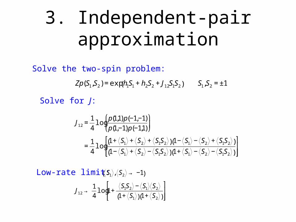
3. Independent-pair approximation

3. Independent-pair approximation
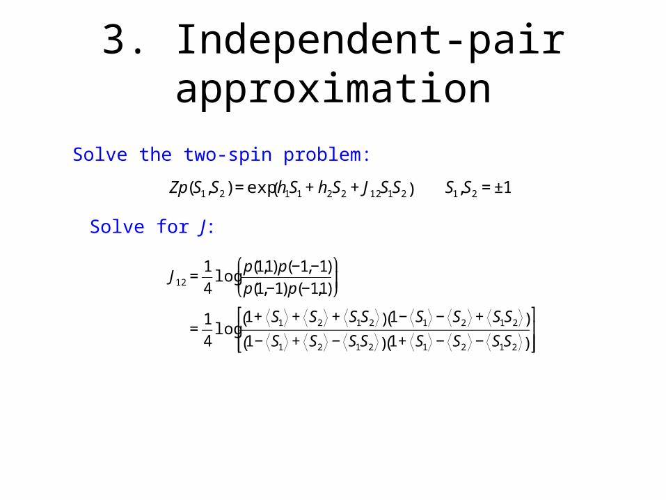
Solve the two-spin problem:
€
Zp(S1,S2) = exp h1S1 + h2S2 + J12S1S2( ) S1,S2 = ±1
3. Independent-pair approximation
Solve the two-spin problem:
€
Zp(S1,S2) = exp h1S1 + h2S2 + J12S1S2( ) S1,S2 = ±1
Solve for J:
€
J12 =1
4log
p(1,1) p(−1,−1)
p(1,−1)p(−1,1)
⎛
⎝ ⎜
⎞
⎠ ⎟
=1
4log
1+ S1 + S2 + S1S2( ) 1− S1 − S2 + S1S2( )
1− S1 + S2 − S1S2( ) 1+ S1 − S2 − S1S2( )
⎡
⎣ ⎢ ⎢
⎤
⎦ ⎥ ⎥
3. Independent-pair approximation
Solve the two-spin problem:
€
Zp(S1,S2) = exp h1S1 + h2S2 + J12S1S2( ) S1,S2 = ±1
Solve for J:
€
J12 =1
4log
p(1,1) p(−1,−1)
p(1,−1)p(−1,1)
⎛
⎝ ⎜
⎞
⎠ ⎟
=1
4log
1+ S1 + S2 + S1S2( ) 1− S1 − S2 + S1S2( )
1− S1 + S2 − S1S2( ) 1+ S1 − S2 − S1S2( )
⎡
⎣ ⎢ ⎢
⎤
⎦ ⎥ ⎥
Low-rate limit:
€
S1 , S2 → −1( )
J12 →1
4log 1+
S1S2 − S1 S2
1+ S1( ) 1+ S2( )
⎡
⎣ ⎢ ⎢
⎤
⎦ ⎥ ⎥
4. Sessak-Monasson approximation
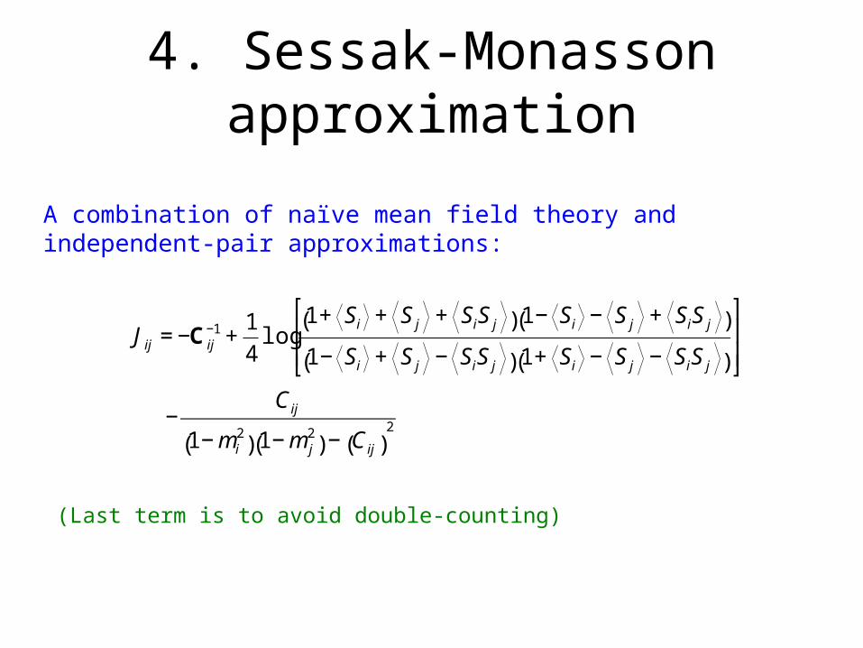
4. Sessak-Monasson approximation
A combination of naïve mean field theory and independent-pair approximations:

4. Sessak-Monasson approximation
A combination of naïve mean field theory and independent-pair approximations:
€
Jij = −Cij−1 +
1
4log
1+ Si + S j + SiS j( ) 1− Si − S j + SiS j( )
1− Si + S j − SiS j( ) 1+ Si − S j − SiS j( )
⎡
⎣
⎢ ⎢
⎤
⎦
⎥ ⎥
−Cij
1− mi2
( ) 1− m j2
( ) − Cij( )2
4. Sessak-Monasson approximation
A combination of naïve mean field theory and independent-pair approximations:
€
Jij = −Cij−1 +
1
4log
1+ Si + S j + SiS j( ) 1− Si − S j + SiS j( )
1− Si + S j − SiS j( ) 1+ Si − S j − SiS j( )
⎡
⎣
⎢ ⎢
⎤
⎦
⎥ ⎥
−Cij
1− mi2
( ) 1− m j2
( ) − Cij( )2
(Last term is to avoid double-counting)
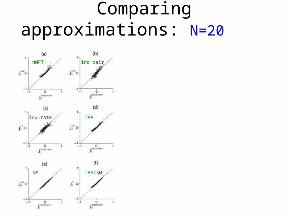
Comparing approximations: N=20
nMFT ind pair
low-rate TAP
SM TAP/SM
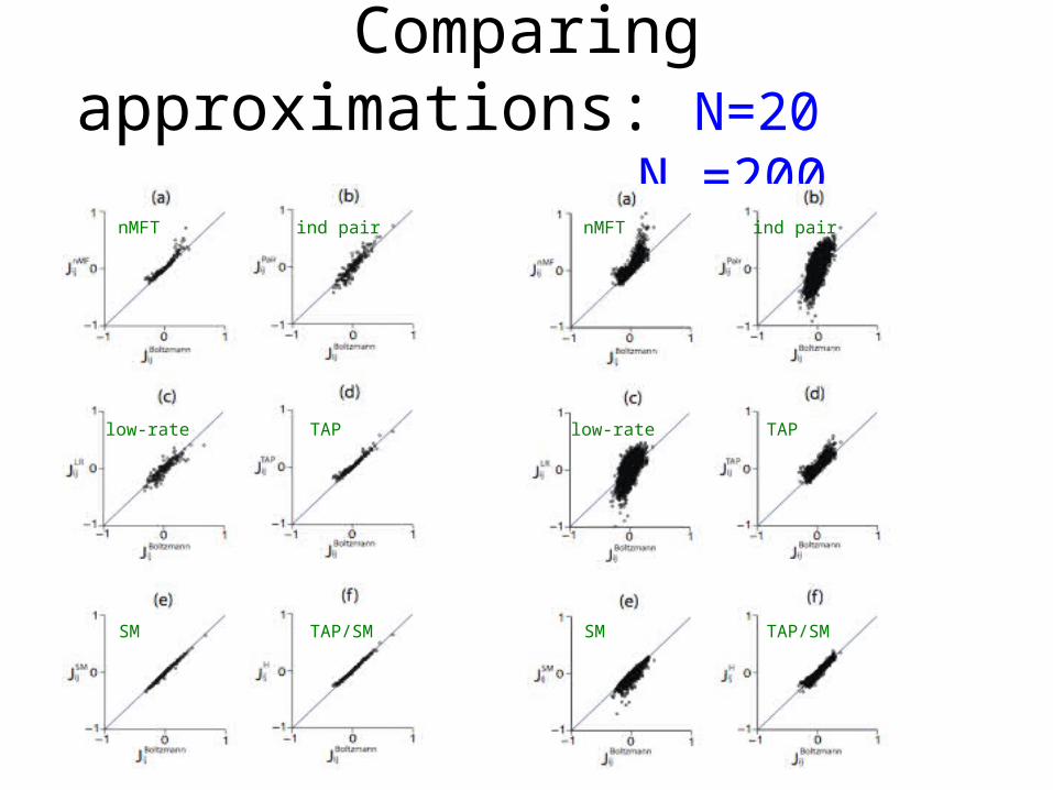
Comparing approximations: N=20 N =200
nMFT ind pair nMFT ind pair
low-rate low-rateTAP TAP
SM SMTAP/SM TAP/SM
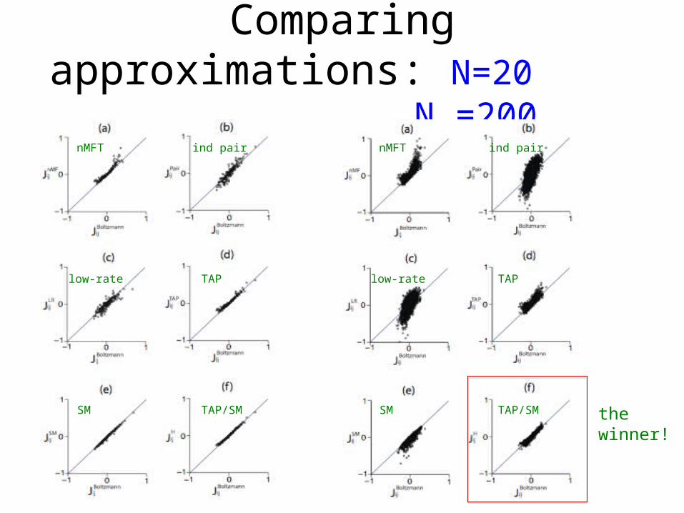
Comparing approximations: N=20 N =200
nMFT ind pair nMFT ind pair
low-rate low-rateTAP TAP
SM SMTAP/SM TAP/SM thewinner!
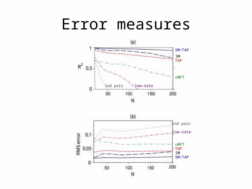
Error measures
SM/TAP
SM
SM/TAPSM
TAP
TAP
nMFT
nMFT
low-rate
low-rate
ind pair
ind pair
N-dependence:How do the inferred couplings depend on the size of the set of neurons used in the inference algorithm?

N-dependence:How do the inferred couplings depend on the size of the set of neurons used in the inference algorithm?
N = 20
N=200
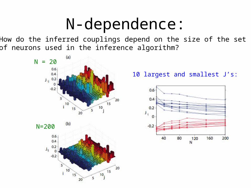
N-dependence:How do the inferred couplings depend on the size of the set of neurons used in the inference algorithm?
N = 20
N=200
10 largest and smallest J’s:

N-dependence:How do the inferred couplings depend on the size of the set of neurons used in the inference algorithm?
N = 20
N=200
10 largest and smallest J’s:
Relative sizes of differentJ’s preserved, absolute sizesshrink.
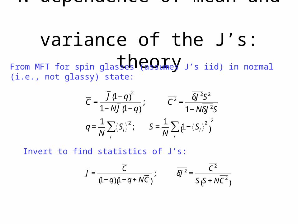
N-dependence of mean and variance of the J’s: theory
N-dependence of mean and variance of the J’s: theoryFrom MFT for spin glasses (assumes J’s iid) in normal (i.e., not glassy) state:
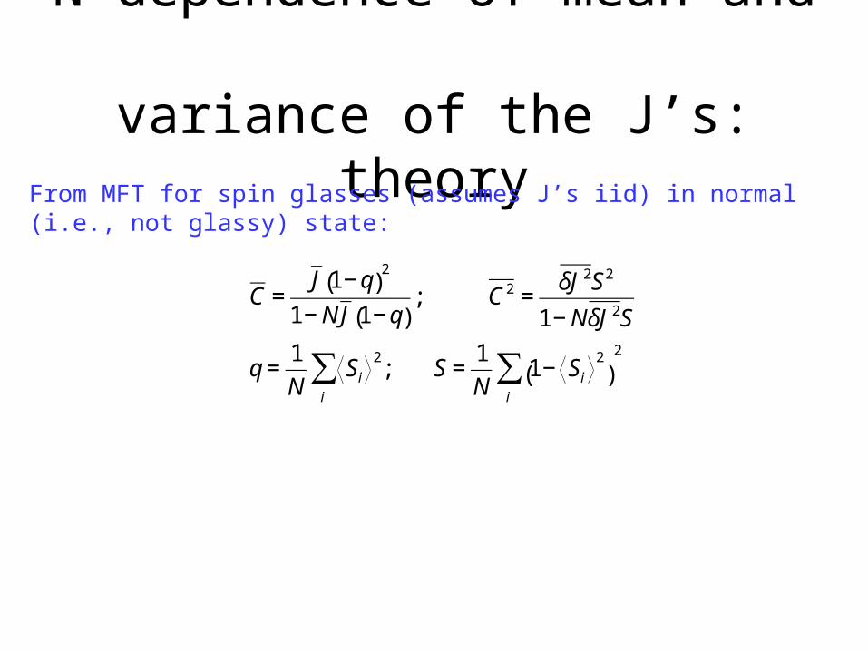
N-dependence of mean and variance of the J’s: theoryFrom MFT for spin glasses (assumes J’s iid) in normal (i.e., not glassy) state:
€
C =J 1− q( )
2
1− NJ 1− q( ); C2 =
δJ 2S2
1− NδJ 2S
q =1
NSi
2
i
∑ ; S =1
N1− Si
2
( )i
∑2
N-dependence of mean and variance of the J’s: theoryFrom MFT for spin glasses (assumes J’s iid) in normal (i.e., not glassy) state:
€
C =J 1− q( )
2
1− NJ 1− q( ); C2 =
δJ 2S2
1− NδJ 2S
q =1
NSi
2
i
∑ ; S =1
N1− Si
2
( )i
∑2
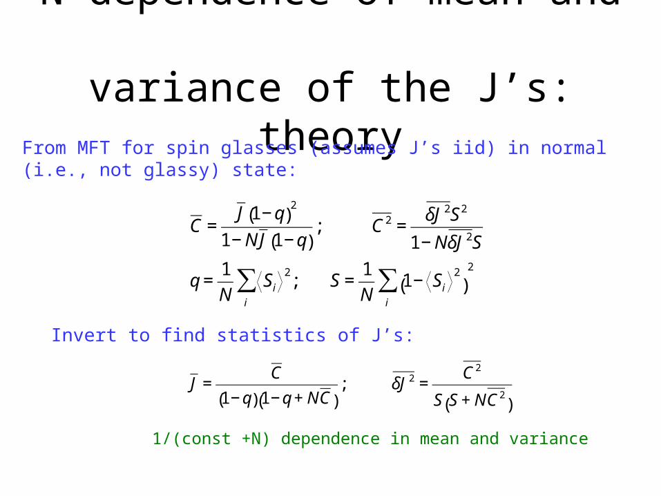
Invert to find statistics of J’s:
€
J =C
1− q( ) 1− q + NC( ); δJ 2 =
C2
S S + NC2( )
N-dependence of mean and variance of the J’s: theoryFrom MFT for spin glasses (assumes J’s iid) in normal (i.e., not glassy) state:
€
C =J 1− q( )
2
1− NJ 1− q( ); C2 =
δJ 2S2
1− NδJ 2S
q =1
NSi
2
i
∑ ; S =1
N1− Si
2
( )i
∑2
Invert to find statistics of J’s:
€
J =C
1− q( ) 1− q + NC( ); δJ 2 =
C2
S S + NC2( )
1/(const +N) dependence in mean and variance
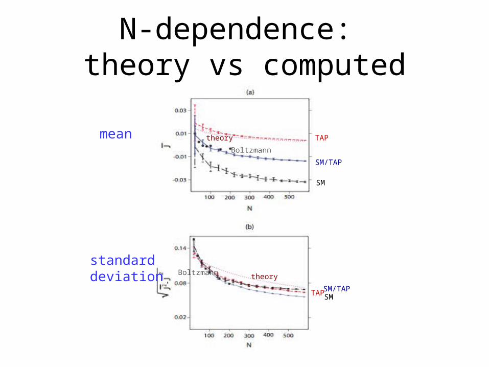
N-dependence: theory vs computed
mean
standarddeviation
TAP
TAP
SM/TAP
SM/TAP
SM
SM
theory
theory
Boltzmann
Boltzmann

Heading for a spin glass state?
Heading for a spin glass state?
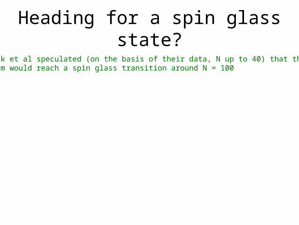
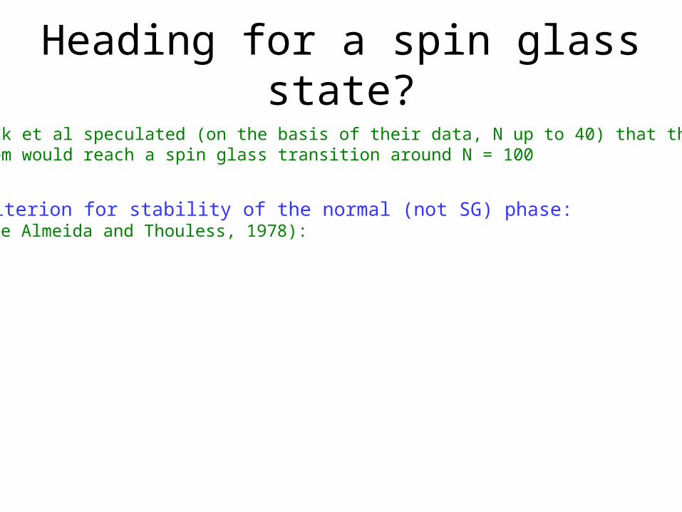
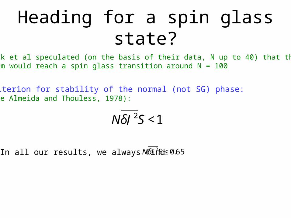
Tkacik et al speculated (on the basis of their data, N up to 40) that thesystem would reach a spin glass transition around N = 100
Heading for a spin glass state?
Tkacik et al speculated (on the basis of their data, N up to 40) that thesystem would reach a spin glass transition around N = 100
Criterion for stability of the normal (not SG) phase: (de Almeida and Thouless, 1978):

Heading for a spin glass state?
Tkacik et al speculated (on the basis of their data, N up to 40) that thesystem would reach a spin glass transition around N = 100
Criterion for stability of the normal (not SG) phase: (de Almeida and Thouless, 1978):
€
NδJ 2S <1
Heading for a spin glass state?
Tkacik et al speculated (on the basis of their data, N up to 40) that thesystem would reach a spin glass transition around N = 100
Criterion for stability of the normal (not SG) phase: (de Almeida and Thouless, 1978):
€
NδJ 2S <1
In all our results, we always find
€
NδJ 2S ≤ 0.65
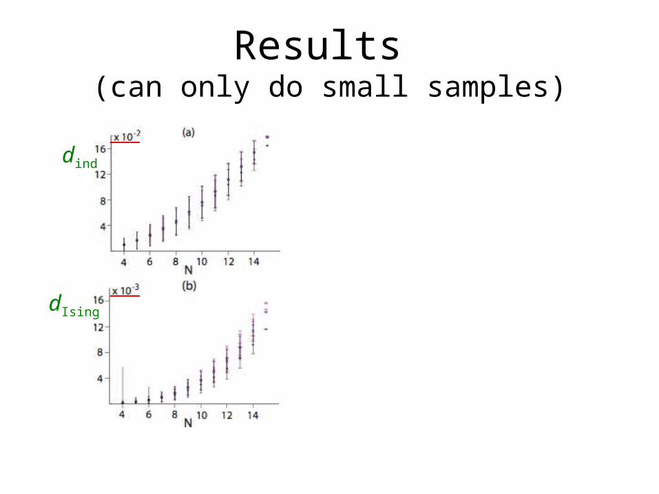
Quality of the Ising-model fit
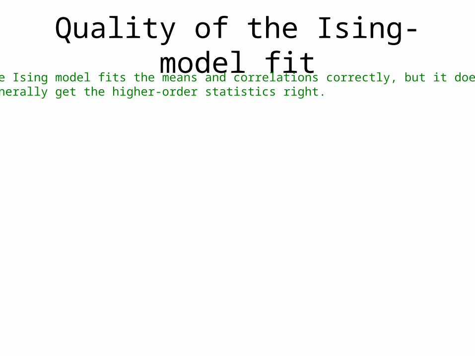
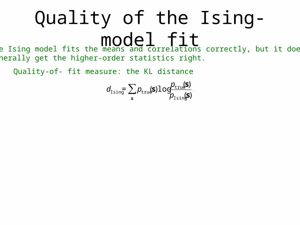
Quality of the Ising-model fitThe Ising model fits the means and correlations correctly, but it does not generally get the higher-order statistics right.
Quality of the Ising-model fitThe Ising model fits the means and correlations correctly, but it does not generally get the higher-order statistics right.
€
dIsing = ptrue(s)logptrue(s)
pIsing(s)s
∑ .
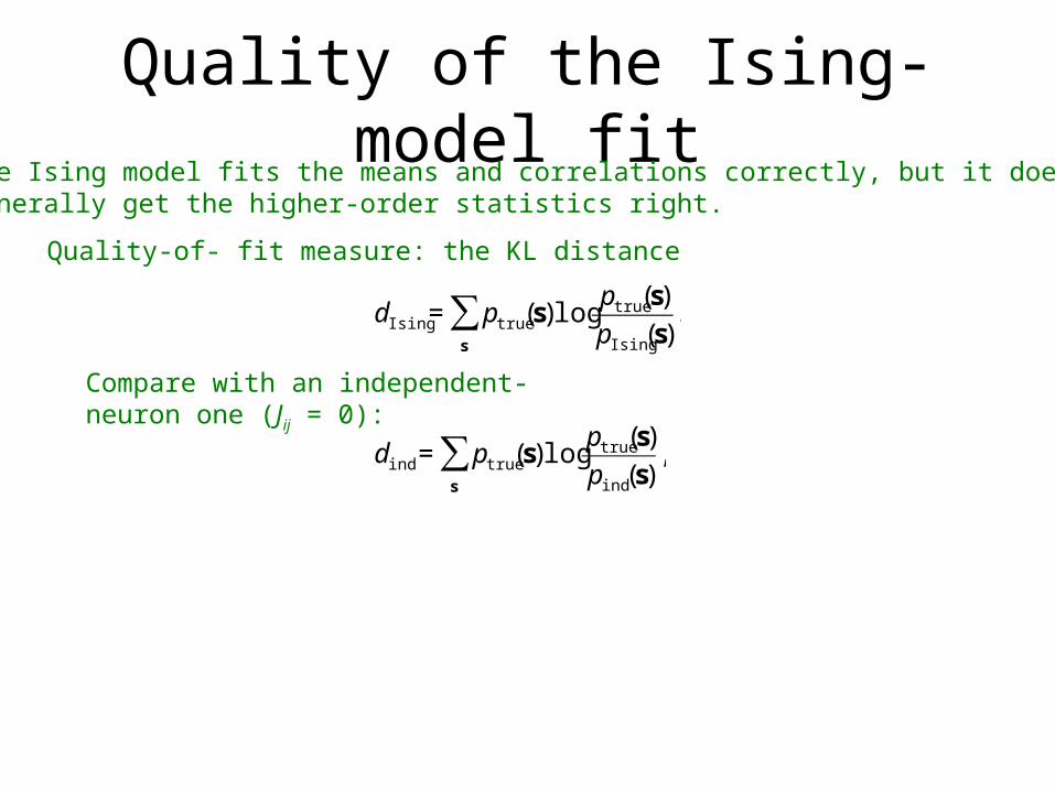
Quality-of- fit measure: the KL distance
Quality of the Ising-model fitThe Ising model fits the means and correlations correctly, but it does not generally get the higher-order statistics right.
€
dIsing = ptrue(s)logptrue(s)
pIsing(s)s
∑ .
Quality-of- fit measure: the KL distance
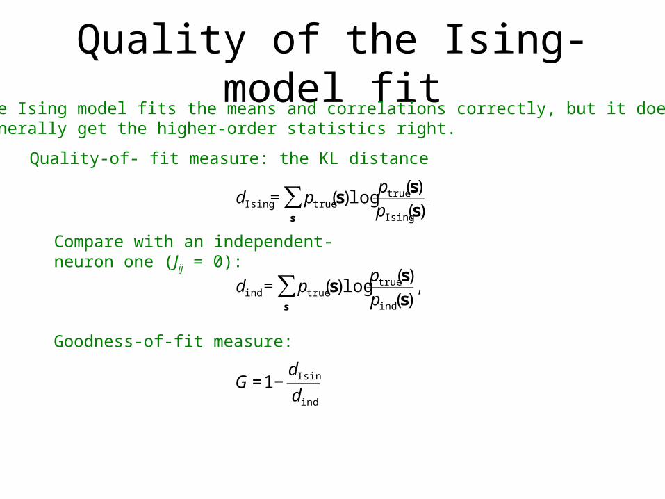
Compare with an independent-neuron one (Jij = 0):
€
dind = ptrue(s)logptrue(s)
pind (s),
s
∑
Quality of the Ising-model fitThe Ising model fits the means and correlations correctly, but it does not generally get the higher-order statistics right.
€
dIsing = ptrue(s)logptrue(s)
pIsing(s)s
∑ .
Quality-of- fit measure: the KL distance
Compare with an independent-neuron one (Jij = 0):
€
dind = ptrue(s)logptrue(s)
pind (s),
s
∑
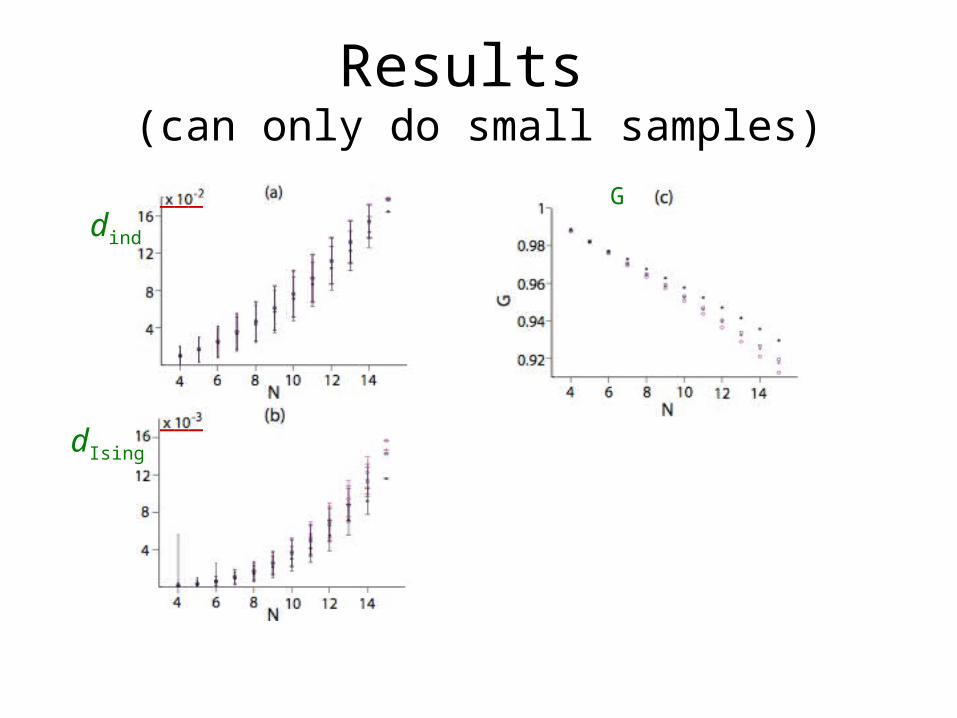
Goodness-of-fit measure:
€
G =1−dIsing
dind
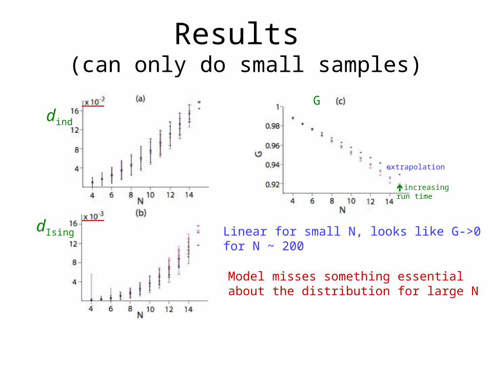
Results (can only do small samples)

Results (can only do small samples)
dIsing
dind
Results (can only do small samples)
dIsing
dind
___
___
Results (can only do small samples)
dIsing
dind
___
___
G
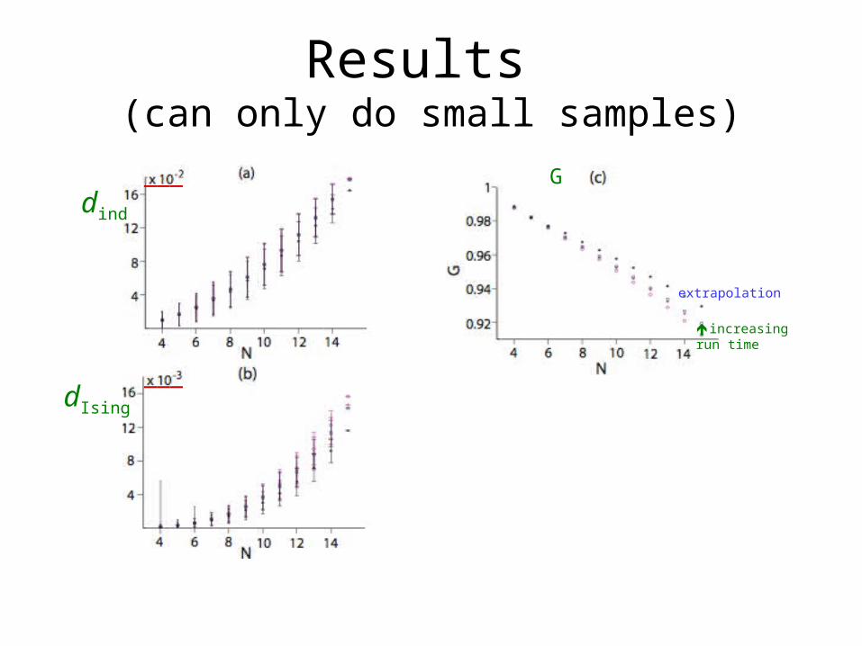
Results (can only do small samples)
dIsing
dind
increasingrun time
extrapolation
___
___
G

Results (can only do small samples)
dIsing
dind
increasingrun time
extrapolation
Linear for small N, looks like G->0for N ~ 200
___
___
G
Results (can only do small samples)
dIsing
dind
increasingrun time
extrapolation
Linear for small N, looks like G->0for N ~ 200
___
___
G
Model misses something essentialabout the distribution for large N
Summary
Summary
• Ising distribution fits means and correlations of neuronal firing

Summary
• Ising distribution fits means and correlations of neuronal firing
• TAP and SM approximations give good, fast estimates of functional couplings Jij
Summary
• Ising distribution fits means and correlations of neuronal firing
• TAP and SM approximations give good, fast estimates of functional couplings Jij
• Spin glass MFT describes scaling of Jij’s with sample size N

Summary
• Ising distribution fits means and correlations of neuronal firing
• TAP and SM approximations give good, fast estimates of functional couplings Jij
• Spin glass MFT describes scaling of Jij’s with sample size N
• Quality of fit to data distribution deteriorates as N grows
Summary
• Ising distribution fits means and correlations of neuronal firing
• TAP and SM approximations give good, fast estimates of functional couplings Jij
• Spin glass MFT describes scaling of Jij’s with sample size N
• Quality of fit to data distribution deteriorates as N growsRead more at arXiv:0902.2885v1 (2009)


