
HAL Id: tel-02272817https://tel.archives-ouvertes.fr/tel-02272817
Submitted on 28 Aug 2019
HAL is a multi-disciplinary open accessarchive for the deposit and dissemination of sci-entific research documents, whether they are pub-lished or not. The documents may come fromteaching and research institutions in France orabroad, or from public or private research centers.
L’archive ouverte pluridisciplinaire HAL, estdestinée au dépôt et à la diffusion de documentsscientifiques de niveau recherche, publiés ou non,émanant des établissements d’enseignement et derecherche français ou étrangers, des laboratoirespublics ou privés.
Isogeometric methods for hyperbolic partial differentialequations
Asma Gdhami
To cite this version:Asma Gdhami. Isogeometric methods for hyperbolic partial differential equations. Analysis of PDEs[math.AP]. COMUE Université Côte d’Azur (2015 - 2019); Université de Tunis El Manar, 2018.English. NNT : 2018AZUR4210. tel-02272817

Méthodes isogéométriques pour les équations aux
dérivées partielles hyperboliques
Asma GDHAMI INRIA -LAMSIN
Présentée en vue de l’obtention
du grade de docteur en Mathématiques
d’Université Côte d’Azur
et de l’Université de Tunis El Manar
Dirigée par: Regis DUVIGNEAU /
Maher MOAKHER
Soutenue le : 17-12-2018
Devant le jury, composé de :
Amel BEN ABDA, Professeur, Université de
Tunis El Manar
Christophe CHALONS, Professeur, Université
de Versailles
Regis DUVIGNEAU, Chargé de Recherche,
INRIA, Université Cote d’Azur
Maatoug HASSINE, Professeur, Université de
Monastir
Maher MOAKHER, Professeur, ENIT,
Université de Tunis El Manar
Claire SCHEID, Maître de conférences,
Université Cote d’Azur
EMPLACEMENT LOGO CO-TUTELLE ÉVENTUELLE
THÈSE DE DOCTORAT

MÉTHODES ISOGÉOMÉTRIQUES POUR LES ÉQUATIONS
AUX DÉRIVÉES PARTIELLES HYPERBOLIQUES
Jury:
Rapporteurs:
Mr. Christophe CHALONS, Professeur, Université de Versailles.
Mr. Maatoug HASSINE, Professeur, Université de Monastir.
Examinateurs:
Mrs. Amel BEN ABDA, Professeur, ENIT, Université de Tunis El Manar.
Mrs. Claire SCHEID, Maître de conférences, Université de Cote Azur.
Mr. Regis DUVIGNEAU, Chargé de Recherche, INRIA, Université de Cote Azur.
Mr. Maher MOAKHER, Professeur, ENIT, Université de Tunis El Manar.
i
MÉTHODES ISOGÉOMÉTRIQUES POUR LES ÉQUATIONS
AUX DÉRIVÉES PARTIELLES HYPERBOLIQUES
REsumé: L’nalyse isogéométrique (AIG) est une méthode innovante de résolution
numérique des équations différentielles, proposée à l’origine par Thomas Hughes,
Austin Cottrell et Yuri Bazilevs en 2005. Cette technique de discrétisation est une
généralisation de l’analyse par éléments finis classiques (AEF), conçue pour intégrer la conception assistée
par ordinateur (CAO), afin de combler l’écart entre la description géométrique et l’analyse des problèmes
d’ingénierie. Ceci est réalisé en utilisant des B-splines ou des B-splines rationnelles non uniformes (NURBS),
pour la description des géométries ainsi que pour la représentation de champs de solutions inconnus.
L’objet de cette thèse est d’étudier la méthode isogéométrique dans le contexte des problèmes hy-
perboliques en utilisant les fonctions B-splines comme fonctions de base. Nous proposons également une
méthode combinant l’AIG avec la méthode de Galerkin discontinue (GD) pour résoudre les problèmes hy-
perboliques. Plus précisément, la méthodologie de GD est adoptée à travers les interfaces de patches, tandis
que l’AIG traditionnelle est utilisée dans chaque patch. Notre méthode tire parti de la méthode de l’AIG et
la méthode de GD.
Les résultats numériques sont présentés jusqu’à l’ordre polynomial p = 4 à la fois pour une méthode de
Galerkin continue et discontinue. Ces résultats numériques sont comparés pour un ensemble de prob-
lèmes de complexité croissante en 1D et 2D .
Mots clés: problèmes hyperboliques, méthode des éléments finis, méthode de Galerkin discontinue,
analyse isogéométrique, fonctions B-splines, extraction de Bézier, ajustement des courbes, méthode de
moindres carrés.
ii

ISOGEOMETRIC METHODS FOR HYPERBOLIC PARTIAL
DIFFERENTIAL EQUATIONS
ABstract: Isogeometric Analysis (IGA) is a modern strategy for numerical solution of
partial differential equations, originally proposed by Thomas Hughes, Austin Cot-
trell and Yuri Bazilevs in 2005. This discretization technique is a generalization
of classical finite element analysis (FEA), designed to integrate Computer Aided Design (CAD) and FEA,
to close the gap between the geometrical description and the analysis of engineering problems. This is
achieved by using B-splines or non-uniform rational B-splines (NURBS), for the description of geometries
as well as for the representation of unknown solution fields.
The purpose of this thesis is to study isogeometric methods in the context of hyperbolic problems using
B-splines as basis functions. We also propose a method that combines IGA with the discontinuous Galerkin
(DG) method for solving hyperbolic problems. More precisely, DG methodology is adopted across the patch
interfaces, while the traditional IGA is employed within each patch. The proposed method takes advantage
of both IGA and the DG method.
Numerical results are presented up to polynomial order p = 4 both for a continuous and discontinuous
Galerkin method. These numerical results are compared for a range of problems of increasing complexity,
in 1D and 2D .
Keywords: hyperbolic problems, Finite Element method, discontinuous Galerkin method, Isogeo-
metric analysis, B-spline functions, Bézier extraction, curve fitting, least squares method.
iii


TO
My dear father Mohamed and my sweet mother Kawther,
for your patience, sacrifices and encouragement.
My husband Aymen, I am more thankful than I can pos-
sibly put down in words, for giving me energy when mine
is running low, for having an open ear for my worries and
my successes, for your faith in me, and above all, for your
closeness and your love.
My son Dali, for making me smile even on the toughest
days.
My sister Haifa & my brother Maher, for your kindness,
your love and your concern.
My aunts Emna & Raoudha and my mother in law Jalila
All my friends, for friendship, love and moments spent
together.
"Nothing is lost, everything is transformed."
Antoine Lavoisier


ACKNOWLEDGMENTS
THese PhD years have been a rich experience from the professional as well as the personal points
of view.
First of all I would like to express my gratitude to my supervisors, Regis Duvigneau & Maher Moakher
for inspiring me, introducing me to new challenges and for helping me carry out this work. I would like to
thank them for showing much interest in my work, and for their help and support at the frequently advising
sessions. At your sides, I have learnt a lot. You shared with me your technical knowledges and above all your
scientific rigorous. In particular, thanks to you, I got the opportunity to attend international congresses.
It represents a lot to me. I would like to express my sincere thanks for your patience, your help, your reg-
ular availability and your encouragement and advice. I dedicate this work to you reflecting my deep respect.
I express my heartfelt thanks to Mrs. Amel BEN ABDA & Mrs. Claire SCHEID for being my thesis
examiner and providing valuable suggestions and corrections.
Also, I present my highly express of thanks to Sir Christophe CHALONS & Sir Maatoug HASSINE for
agreeing to be the reviewers of my work and for your constructive suggestions.
Then, I address a special appreciation for Sir. Mekki Ayadi that helped me to accomplish this work by
extensive discussions. I would like to express my sincere thanks for your patience, your help, your encour-
agement and advice.
My next big thank you is to my families Gdhami, Essid and Azaouzi. To my parents Mohamed and
Kaouther, my brother and my sister for their unconditional love and support all though my life. To them I
owe all that I am and all that I have ever accomplished and it is to them I dedicate this thesis. Moreover, I
will never forget my cousins Sana, Ichraf, Boutheina, Soumaya & Olfa who have always encouraged me to
accomplish my studies.
vii

On a more personal note, I would like to express my deep gratitude to my husband Aymen for his sup-
port. This work is dedicated to him and to my son with my deepest love.
I address a special message for my second family: my friends from the Modeling Laboratory in Engi-
neering Sciences (LAMSIN) National Engineering School of Tunis (ENIT), Boutheina, Imen, Rabeb, Maroua,
hamouda, Anis, ... and my friends of the National Institute for Research in Computer Science and Automatic
of Nice (INRIA), I would like to express my gratitude for their continuous encouragement.
In the life path, we meet people that can change our life in a different measure - some change it
forever. I am sure I would have forgotten some people in this acknowledgement section, that is why for the
sake of completion I am thanking all the people who shared with me parts of these years. Thanks for being
part of my path. In a certain way, that you maybe do not measure, you contribute to allow me to arrive here
today.
viii
TABLE OF CONTENTS
Résumé ii
Abstract iii
Acknowledgments vii
List of Tables xiv
List of Figures xvii
List of Abbreviations xxi
List of Symbols xxiii
1 Introduction 1
I CAD REPRESENTATIONS 14
2 Bézier Curves 16
2.1 Bernstein basis . . . . . . . . . . . . . . . . . . . . . . . . . . . . . . . . . . . . . . . . . . . . . . 16
2.2 Properties of the Bernstein polynomials . . . . . . . . . . . . . . . . . . . . . . . . . . . . . . . 19
2.3 Derivatives . . . . . . . . . . . . . . . . . . . . . . . . . . . . . . . . . . . . . . . . . . . . . . . . . 21
2.4 Bézier curves . . . . . . . . . . . . . . . . . . . . . . . . . . . . . . . . . . . . . . . . . . . . . . . . 22
2.5 Properties . . . . . . . . . . . . . . . . . . . . . . . . . . . . . . . . . . . . . . . . . . . . . . . . . 22
2.5.1 Degree elevation . . . . . . . . . . . . . . . . . . . . . . . . . . . . . . . . . . . . . . . . . 25
2.5.2 Derivatives of a Bézier Curve . . . . . . . . . . . . . . . . . . . . . . . . . . . . . . . . . 26
2.6 Subdivision of Bézier curves . . . . . . . . . . . . . . . . . . . . . . . . . . . . . . . . . . . . . . 28
2.7 Rational Bézier curves . . . . . . . . . . . . . . . . . . . . . . . . . . . . . . . . . . . . . . . . . . 29
2.8 Bézier surface . . . . . . . . . . . . . . . . . . . . . . . . . . . . . . . . . . . . . . . . . . . . . . . 30
3 B-splines curves 34
3.1 B-spline functions . . . . . . . . . . . . . . . . . . . . . . . . . . . . . . . . . . . . . . . . . . . . 34
3.1.1 Knot Vectors . . . . . . . . . . . . . . . . . . . . . . . . . . . . . . . . . . . . . . . . . . . 36
ix

TABLE OF CONTENTS
3.1.2 Properties of the B-spline functions . . . . . . . . . . . . . . . . . . . . . . . . . . . . . 38
3.2 Derivatives of B-spline functions . . . . . . . . . . . . . . . . . . . . . . . . . . . . . . . . . . . . 39
3.3 B-spline curves . . . . . . . . . . . . . . . . . . . . . . . . . . . . . . . . . . . . . . . . . . . . . . 41
3.4 Hierarchical representation . . . . . . . . . . . . . . . . . . . . . . . . . . . . . . . . . . . . . . . 43
3.4.1 Knot insertion . . . . . . . . . . . . . . . . . . . . . . . . . . . . . . . . . . . . . . . . . . 43
3.4.2 Order elevation . . . . . . . . . . . . . . . . . . . . . . . . . . . . . . . . . . . . . . . . . . 44
3.4.3 k−refinement . . . . . . . . . . . . . . . . . . . . . . . . . . . . . . . . . . . . . . . . . . 44
3.5 B-spline surfaces and volumes . . . . . . . . . . . . . . . . . . . . . . . . . . . . . . . . . . . . . 45
3.6 Non-Uniform Rational B-spline (NURBS) . . . . . . . . . . . . . . . . . . . . . . . . . . . . . . 46
3.6.1 NURBS basis functions . . . . . . . . . . . . . . . . . . . . . . . . . . . . . . . . . . . . . 46
3.6.2 NURBS curves and surfaces . . . . . . . . . . . . . . . . . . . . . . . . . . . . . . . . . . 46
3.7 Extracting Bézier curves from B-splines . . . . . . . . . . . . . . . . . . . . . . . . . . . . . . . 47
4 Curve and surface fitting 52
4.1 Curve fitting . . . . . . . . . . . . . . . . . . . . . . . . . . . . . . . . . . . . . . . . . . . . . . . . 52
4.1.1 Basic concepts . . . . . . . . . . . . . . . . . . . . . . . . . . . . . . . . . . . . . . . . . . 52
4.1.2 Description of the least squares method . . . . . . . . . . . . . . . . . . . . . . . . . . 53
4.2 B-spline curve fitting - example . . . . . . . . . . . . . . . . . . . . . . . . . . . . . . . . . . . . 54
4.3 Least-squares B-spline surface fitting . . . . . . . . . . . . . . . . . . . . . . . . . . . . . . . . . 55
4.4 B-spline surface fitting - examples . . . . . . . . . . . . . . . . . . . . . . . . . . . . . . . . . . . 57
II ISOGEOMETRIC ANALYSIS - FINITE ELEMENT FRAMEWORK (ILLUSTRATION FOR A
1D PROBLEM) 63
5 SUPG - FINITE ELEMENT METHOD 65
5.1 Preliminaries . . . . . . . . . . . . . . . . . . . . . . . . . . . . . . . . . . . . . . . . . . . . . . . 65
5.2 Standard Galerkin FEM . . . . . . . . . . . . . . . . . . . . . . . . . . . . . . . . . . . . . . . . . 66
5.3 Lagrange P1 elements . . . . . . . . . . . . . . . . . . . . . . . . . . . . . . . . . . . . . . . . . . 67
5.4 SUPG FEM for one-dimensional linear advection problem . . . . . . . . . . . . . . . . . . . . 73
5.4.1 Selection of the SUPG stabilization parameter . . . . . . . . . . . . . . . . . . . . . . . 73
5.4.2 SUPG finite element approximation . . . . . . . . . . . . . . . . . . . . . . . . . . . . . 74
5.4.3 Mass lumping . . . . . . . . . . . . . . . . . . . . . . . . . . . . . . . . . . . . . . . . . . 76
5.4.4 Runge-Kutta time discretization . . . . . . . . . . . . . . . . . . . . . . . . . . . . . . . 77
5.4.5 Courant-Friedrichs-Lewy (CFL) condition . . . . . . . . . . . . . . . . . . . . . . . . . 79
5.5 Numerical results . . . . . . . . . . . . . . . . . . . . . . . . . . . . . . . . . . . . . . . . . . . . . 79
5.5.1 Influence of the SUPG parameter . . . . . . . . . . . . . . . . . . . . . . . . . . . . . . . 80
5.5.2 Error Estimates for the SUPG FE method . . . . . . . . . . . . . . . . . . . . . . . . . . 81
5.6 SUPG FE method for high-order elements . . . . . . . . . . . . . . . . . . . . . . . . . . . . . . 83
5.6.1 Matrix assembly . . . . . . . . . . . . . . . . . . . . . . . . . . . . . . . . . . . . . . . . . 87
x

TABLE OF CONTENTS
5.6.2 Numerical results . . . . . . . . . . . . . . . . . . . . . . . . . . . . . . . . . . . . . . . . 88
5.6.3 Accuracy study . . . . . . . . . . . . . . . . . . . . . . . . . . . . . . . . . . . . . . . . . . 89
5.7 Conclusion . . . . . . . . . . . . . . . . . . . . . . . . . . . . . . . . . . . . . . . . . . . . . . . . . 90
6 Isogeometric Analysis: B-spline as a FEM basis 94
6.1 IGA: a B-spline based approach . . . . . . . . . . . . . . . . . . . . . . . . . . . . . . . . . . . . 94
6.1.1 Isogeometric discretisation . . . . . . . . . . . . . . . . . . . . . . . . . . . . . . . . . . 95
6.1.2 Computational procedures for IGA . . . . . . . . . . . . . . . . . . . . . . . . . . . . . . 96
6.2 Isogeometric FE formulation . . . . . . . . . . . . . . . . . . . . . . . . . . . . . . . . . . . . . . 97
6.3 Numerical results . . . . . . . . . . . . . . . . . . . . . . . . . . . . . . . . . . . . . . . . . . . . . 101
6.3.1 Influence of the SUPG stabilization parameter τ for the quadratic B-spline . . . . . 102
6.3.2 Error estimates for the quadratic B-spline . . . . . . . . . . . . . . . . . . . . . . . . . 103
6.4 Higher order B-spline . . . . . . . . . . . . . . . . . . . . . . . . . . . . . . . . . . . . . . . . . . 104
6.5 IGFEA and classical FEA: a comparisons . . . . . . . . . . . . . . . . . . . . . . . . . . . . . . . 105
III ISOGEOMETRIC DISCONTINUOUS GALERKIN METHOD (IGDGM) 110
7 Discontinuous Galerkin Method (DGM): from classical to isogeometric 111
7.1 Introduction and background . . . . . . . . . . . . . . . . . . . . . . . . . . . . . . . . . . . . . 111
7.2 DGFE framework for one-dimensional scalar conservation law . . . . . . . . . . . . . . . . . 112
7.2.1 Discontinuous Galerkin-space discretization . . . . . . . . . . . . . . . . . . . . . . . 112
7.2.2 Numerical flux . . . . . . . . . . . . . . . . . . . . . . . . . . . . . . . . . . . . . . . . . . 114
7.2.3 Elementary linear system . . . . . . . . . . . . . . . . . . . . . . . . . . . . . . . . . . . 115
7.3 Computation of residual and mass matrix . . . . . . . . . . . . . . . . . . . . . . . . . . . . . . 116
7.4 CFL condition for DG Method . . . . . . . . . . . . . . . . . . . . . . . . . . . . . . . . . . . . . 116
7.5 Numerical results . . . . . . . . . . . . . . . . . . . . . . . . . . . . . . . . . . . . . . . . . . . . . 117
7.6 Isogeometric - discontinuous Galerkin framework (IGDG) . . . . . . . . . . . . . . . . . . . . 119
7.6.1 Construction of the DG basis . . . . . . . . . . . . . . . . . . . . . . . . . . . . . . . . . 119
7.6.2 Isogeometric discontinuous Galerkin approximation spaces . . . . . . . . . . . . . . 121
7.6.3 Computation of residual and mass matrix . . . . . . . . . . . . . . . . . . . . . . . . . 122
7.7 Numerical studies . . . . . . . . . . . . . . . . . . . . . . . . . . . . . . . . . . . . . . . . . . . . . 123
7.8 Conclusion and comparison . . . . . . . . . . . . . . . . . . . . . . . . . . . . . . . . . . . . . . 126
IV 2D PROBLEM STUDY 131
8 IGDG: 2D Advection Problem 132
8.1 Computational procedures in two dimensions . . . . . . . . . . . . . . . . . . . . . . . . . . . 132
8.1.1 Preliminaries - IGDG notation . . . . . . . . . . . . . . . . . . . . . . . . . . . . . . . . 132
8.1.2 Isogeometric analysis (IGA): physical domain and geometrical mappings . . . . . . 132
xi
TABLE OF CONTENTS
8.1.3 Basic function space for the parametric domain and physical domain . . . . . . . . 134
8.1.4 Numerical integration . . . . . . . . . . . . . . . . . . . . . . . . . . . . . . . . . . . . . 135
8.2 2D advection problem: IGDG space semi-discretization . . . . . . . . . . . . . . . . . . . . . 136
8.2.1 Isogeometric discontinuous Galerkin space semi-discretization . . . . . . . . . . . . 137
8.2.2 Elementary linear system . . . . . . . . . . . . . . . . . . . . . . . . . . . . . . . . . . . 137
8.3 Numerical Lax–Friedrichs fluxes . . . . . . . . . . . . . . . . . . . . . . . . . . . . . . . . . . . . 139
8.4 The RK time discretization . . . . . . . . . . . . . . . . . . . . . . . . . . . . . . . . . . . . . . . 140
8.5 Numerical results . . . . . . . . . . . . . . . . . . . . . . . . . . . . . . . . . . . . . . . . . . . . . 140
8.5.1 Cartesian grids . . . . . . . . . . . . . . . . . . . . . . . . . . . . . . . . . . . . . . . . . . 142
8.5.2 Linear grids . . . . . . . . . . . . . . . . . . . . . . . . . . . . . . . . . . . . . . . . . . . . 146
8.5.3 Curvilinear grids . . . . . . . . . . . . . . . . . . . . . . . . . . . . . . . . . . . . . . . . . 149
8.6 Conclusion . . . . . . . . . . . . . . . . . . . . . . . . . . . . . . . . . . . . . . . . . . . . . . . . . 152
9 2D Acoustic wave equations 154
9.1 Introduction and basic theory . . . . . . . . . . . . . . . . . . . . . . . . . . . . . . . . . . . . . 154
9.2 IGDG approximation of the acoustic wave equations . . . . . . . . . . . . . . . . . . . . . . . 155
9.2.1 Spatial discretization . . . . . . . . . . . . . . . . . . . . . . . . . . . . . . . . . . . . . . 155
9.2.2 First variational equation . . . . . . . . . . . . . . . . . . . . . . . . . . . . . . . . . . . 157
9.2.3 Second variational equation . . . . . . . . . . . . . . . . . . . . . . . . . . . . . . . . . . 158
9.2.4 Third variational equation . . . . . . . . . . . . . . . . . . . . . . . . . . . . . . . . . . . 159
9.3 Elementary linear system . . . . . . . . . . . . . . . . . . . . . . . . . . . . . . . . . . . . . . . . 160
9.4 Numerical Lax–Friedrichs fluxes . . . . . . . . . . . . . . . . . . . . . . . . . . . . . . . . . . . . 161
9.5 Numerical results . . . . . . . . . . . . . . . . . . . . . . . . . . . . . . . . . . . . . . . . . . . . . 163
9.5.1 Rectilinear grids . . . . . . . . . . . . . . . . . . . . . . . . . . . . . . . . . . . . . . . . . 166
9.5.2 Curvilinear grids . . . . . . . . . . . . . . . . . . . . . . . . . . . . . . . . . . . . . . . . . 175
9.6 Conclusion . . . . . . . . . . . . . . . . . . . . . . . . . . . . . . . . . . . . . . . . . . . . . . . . . 182
V General Conclusion & Perspectives 186
APPENDICES 193
A 194
Appendix A 194
A.1 Gaussian quadrature . . . . . . . . . . . . . . . . . . . . . . . . . . . . . . . . . . . . . . . . . . . 194
B 196
Appendix B 196
B.1 Runge-Kutta (RK) method: . . . . . . . . . . . . . . . . . . . . . . . . . . . . . . . . . . . . . . . 196
B.2 1D slope limiting . . . . . . . . . . . . . . . . . . . . . . . . . . . . . . . . . . . . . . . . . . . . . 197
xii

TABLE OF CONTENTS
B.2.1 TVDM limiter . . . . . . . . . . . . . . . . . . . . . . . . . . . . . . . . . . . . . . . . . . . 197
B.2.2 TVBM limiter . . . . . . . . . . . . . . . . . . . . . . . . . . . . . . . . . . . . . . . . . . . 198
C 200
Appendix C 200
C.1 Bessel functions zeros . . . . . . . . . . . . . . . . . . . . . . . . . . . . . . . . . . . . . . . . . . 200
Bibliography 202
xiii

LIST OF TABLES
5.1 L2-errors of the SUPG FE P1 method for the one-dimensional advection problem. . . . . . . . . . 82
5.2 Convergence rates. . . . . . . . . . . . . . . . . . . . . . . . . . . . . . . . . . . . . . . . . . . . . . . . 83
5.3 The L2-error norm in function of the choice of the stabilization parameter α. . . . . . . . . . . . . 89
5.4 The L2-error norm for RK 4 time discretization. . . . . . . . . . . . . . . . . . . . . . . . . . . . . . . 90
6.1 The L2-error as function of the choice of the number of control points n and the stabilization
parameter α, for quadratic B-splines in conjunction with RK 2. . . . . . . . . . . . . . . . . . . . . 103
6.2 The L2-error as function of the choice of the number of control points n for quadratic B-splines
in conjunction with RK 4. . . . . . . . . . . . . . . . . . . . . . . . . . . . . . . . . . . . . . . . . . . . 103
6.3 Error measured in the L2-norm. . . . . . . . . . . . . . . . . . . . . . . . . . . . . . . . . . . . . . . . 104
6.4 Convergence rates. . . . . . . . . . . . . . . . . . . . . . . . . . . . . . . . . . . . . . . . . . . . . . . . 104
7.1 L2-errors for the 1D advection problem. . . . . . . . . . . . . . . . . . . . . . . . . . . . . . . . . . . 118
7.2 L2−error for the IGDG method in conjunction with RK 2 time discretisation for various element
sizes and degree of Bézier basis p = 0,1,2. . . . . . . . . . . . . . . . . . . . . . . . . . . . . . . . . . 124
7.3 L2−error for the IGDG method in conjunction with RK 4 time discretisation for various element
sizes and degree of Bézier basis p = 2,3,4. . . . . . . . . . . . . . . . . . . . . . . . . . . . . . . . . . 124
8.1 L2−error for the 2D advection problem and convergence order for the IGDG method for the
linear (left) and quadratic (right) Bernstein bases in conjunction with RK 4 time discretisation. . 144
8.2 L2−error for the 2D advection problem and convergence order for the IGDG method for the
cubic (left) and quartic (right) Bernstein bases in conjunction with RK 4 time discretisation. . . . 144
8.3 L2−error for the 2D advection problem and convergence order for the IGDG method for the
linear (left) and quadratic (right) Bernstein bases in conjunction with RK 4 time discretisation. . 148
8.4 L2−error for the 2D advection problem and convergence order for the IGDG method for the
cubic (left) and quartic (right) Bernstein bases in conjunction with RK 4 time discretisation. . . . 148
8.5 L2−error for the 2D advection problem and convergence order for the IGDG method for the
linear (left) and quadratic (right) Bernstein bases in conjunction with RK 4 time discretisation. . 151
8.6 L2−error for the 2D advection problem vs. mesh parameter and convergence order for the IGDG
method for the cubic (left) and quartic (right) Bernstein bases in conjunction with RK 4 time
discretisation. . . . . . . . . . . . . . . . . . . . . . . . . . . . . . . . . . . . . . . . . . . . . . . . . . . 151
xiv

List of Tables
9.1 L2−error for the 2D acoustic problem and convergence order for the IGDG method for the quadratic
Bernstein bases in conjunction with RK 4 time discretisation. . . . . . . . . . . . . . . . . . . . . . 173
9.2 L2−error for the 2D acoustic problem and convergence order for the IGDG method for the cubic
(left) and quartic (right) Bernstein bases in conjunction with RK 4 time discretisation. . . . . . . . 173
9.3 L2−error for the 2D acoustic problem and convergence order for the IGDG method for the quadratic
Bernstein bases in conjunction with RK 4 time discretisation. . . . . . . . . . . . . . . . . . . . . . 181
9.4 L2−error for the 2D acoustic problem and convergence order for the IGDG method for the cubic
(left) and quartic (right) Bernstein bases in conjunction with RK 4 time discretisation. . . . . . . . 181
A.1 Gauss–Legendre nodes and coefficients . . . . . . . . . . . . . . . . . . . . . . . . . . . . . . . . . . 194
xv


LIST OF FIGURES
2.1 Constant, linear, quadratic and cubic Bernstein polynomials. . . . . . . . . . . . . . . . . . . . . . 17
2.2 Linear, quadratic and cubic bivariate Bernstein polynomials. . . . . . . . . . . . . . . . . . . . . . 18
2.3 Bézier curves of various degrees and their control polygons. . . . . . . . . . . . . . . . . . . . . . . 22
2.4 Bézier curves with endpoint interpolation. . . . . . . . . . . . . . . . . . . . . . . . . . . . . . . . . 23
2.5 Cubic Bézier curve, its control polygon and the convex hull. . . . . . . . . . . . . . . . . . . . . . . 24
2.6 Quadric Bézier curve and repositioning of the control point P2. . . . . . . . . . . . . . . . . . . . . 24
2.7 Degree elevation of a quadratic Bézier Curve. . . . . . . . . . . . . . . . . . . . . . . . . . . . . . . . 26
2.8 Geometric construction according to De Casteljau’s algorithm for p = 3 and ζ= 2/3. . . . . . . . . 28
2.9 Quadratic rational Bézier curves. . . . . . . . . . . . . . . . . . . . . . . . . . . . . . . . . . . . . . . 29
2.10 Tensor product Bézier patch of degree 3×3 and its control net. . . . . . . . . . . . . . . . . . . . . 30
3.1 Basis functions of degrees 1,2 and 3 for uniform knot vector Ξ= 0,1,2,3, .... . . . . . . . . . . . . 35
3.2 Bivariates quadratic and cubic B-spline basis functions [16]. . . . . . . . . . . . . . . . . . . . . . . 36
3.3 Quadratic basis functions for the open-uniform knot vector Ξ= 0,0,0,1,2,3,3,3
. . . . . . . . . . 37
3.4 Quadratic basis functions with reduced continuity at ξ= 1, Ξ= 0,0,0,1,1,2,3,3,3
. . . . . . . . . 38
3.5 Quadratic B-spline curve. . . . . . . . . . . . . . . . . . . . . . . . . . . . . . . . . . . . . . . . . . . . 42
3.6 A quadratic B-spline curve and its control points. In the right, the curve after moving the control
point P4. . . . . . . . . . . . . . . . . . . . . . . . . . . . . . . . . . . . . . . . . . . . . . . . . . . . . . 42
3.7 Before and after knot insertion (cubic B-spline curve). . . . . . . . . . . . . . . . . . . . . . . . . . . 43
3.8 B-spline surface example. . . . . . . . . . . . . . . . . . . . . . . . . . . . . . . . . . . . . . . . . . . . 45
3.9 Bézier decomposition (bottom) from a quadratic B-spline basis (top) by knot insertion. . . . . . . 48
4.1 The least-squares quadratic B-spline curve fitting. . . . . . . . . . . . . . . . . . . . . . . . . . . . . 55
4.2 The least-squares quadratic B-spline Gaussian surface fitting. . . . . . . . . . . . . . . . . . . . . . 57
4.3 Bessel functions of the first kind-1D . . . . . . . . . . . . . . . . . . . . . . . . . . . . . . . . . . . . . 58
4.4 Representation of the physical domainΩ. . . . . . . . . . . . . . . . . . . . . . . . . . . . . . . . . . 58
4.5 The least-squares quadratic B-spline surface fitting. . . . . . . . . . . . . . . . . . . . . . . . . . . . 59
5.1 Uniform P1 mesh of [a,b]. . . . . . . . . . . . . . . . . . . . . . . . . . . . . . . . . . . . . . . . . . . 67
5.2 Global shape functions for the space V 1h . . . . . . . . . . . . . . . . . . . . . . . . . . . . . . . . . . . 68
5.3 The exact sine wave solution for the one-dimensional advection problem. . . . . . . . . . . . . . . 69
xvii

List of Figures
5.4 Exact and standard Galerkin FEM P1 solution for the one-dimensional linear advection problem
at T = 0.4s. . . . . . . . . . . . . . . . . . . . . . . . . . . . . . . . . . . . . . . . . . . . . . . . . . . . 71
5.5 Exact, Galerkin and SUPG solutions at T = 0.4s. . . . . . . . . . . . . . . . . . . . . . . . . . . . . . . 79
5.6 SUPG FE P1 solution for different values of α ∈ [0,1]. . . . . . . . . . . . . . . . . . . . . . . . . . . . 80
5.7 Convergence in number of d.o.f. for different choices of α. . . . . . . . . . . . . . . . . . . . . . . . 82
5.8 Uniform P2 mesh of [a,b]. . . . . . . . . . . . . . . . . . . . . . . . . . . . . . . . . . . . . . . . . . . 83
5.9 Global shape functions for the space V 2h . . . . . . . . . . . . . . . . . . . . . . . . . . . . . . . . . . . 84
5.10 SUPG quadratic Lagrange P2 FEM in conjunction with RK 2 for the 1D advection problem. . . . . 88
5.11 L2-error for the advection problem with the linear and quadratic Lagrange FEM. . . . . . . . . . . 90
6.1 An example of a B-spline patch in physical space Ω, parametric space Ω, and the reference ele-
ment Ω used to perform numerical integration. . . . . . . . . . . . . . . . . . . . . . . . . . . . . . 95
6.2 (a) SUPG B-spline linear solution for the advection problem (α= 0.1). (b) SUPG FEM P1 for the
advection problem (α= 0.1) at T = 0.4s. . . . . . . . . . . . . . . . . . . . . . . . . . . . . . . . . . . 101
6.3 SUPG quadratic B-spline solutions in conjunction with RK 2 for the advection problem. . . . . . 102
6.4 Convergence rates in the L2-norm. . . . . . . . . . . . . . . . . . . . . . . . . . . . . . . . . . . . . . 104
6.5 Error in the L2-norm of IGFEM and classical FEM vs. number of d.o.f. . . . . . . . . . . . . . . . . 105
7.1 L2-errors for the 1D advection problem using the DGFE method in conjunction with the RK
method for a sinusoidal initial condition and Lax-Friedrichs flux. . . . . . . . . . . . . . . . . . . . 118
7.2 Bézier decomposition (bottom) from a quadratic B-spline basis (top) by knot insertion. . . . . . . 120
7.3 IGDG solution of the 1D advection problem for quadratic (a), cubic (b) and quartic (c) basis and
exact solution with 4 Bézier elements. RK 4 time discretization and Lax-Friedrichs flux were used. 123
7.4 L2-errors for the 1D advection problem with a sinusoidal initial condition, RK 2 and RK 4. . . . . 125
7.5 Convergence rates in IGDG method as a function of the Bernstein function is degree p for the
finest grid. . . . . . . . . . . . . . . . . . . . . . . . . . . . . . . . . . . . . . . . . . . . . . . . . . . . . 125
7.6 Error in the L2-norm combining IGFEM, DGFEM, IGDG space discretization and explicit RK time
integration. . . . . . . . . . . . . . . . . . . . . . . . . . . . . . . . . . . . . . . . . . . . . . . . . . . . 127
8.1 An example of a B-spline patch in physical space, parametric space, and the parent element used
to perform numerical integration. . . . . . . . . . . . . . . . . . . . . . . . . . . . . . . . . . . . . . . 133
8.2 Element De , its faces(Γe
k
)k=1,...,4 and the corresponding normals −→n e
|Γek
. . . . . . . . . . . . . . . . . 139
8.3 Analytical solution for the bi-dimensional advection problem, for Nel = 4×4 at T = 0.5s. . . . . . 141
8.4 Plots and contour plots of numerical results for bivariate quadratic Bernstein basis with (a)Nel =4×4 patches and (b) Nel = 8×8 patches at T = 0.05s. . . . . . . . . . . . . . . . . . . . . . . . . . . 142
8.5 IGDG solution for Nel = 8×8 patches for different degrees (p, q). . . . . . . . . . . . . . . . . . . . 143
8.6 L2−error for the 2D advection problem using the IGDG method in conjunction with RK 4. . . . . 145
8.7 Contour plots of numerical results for bivariate quadratic Bernstein basis at T = 0.05s. . . . . . . 146
8.8 IGDG solutions for different degrees for Nel = 8×8 uniform elements. . . . . . . . . . . . . . . . . 147
8.9 L2−error for the 2D advection problem using the IGDG method in conjunction with RK 4. . . . . 148
xviii

List of Figures
8.10 Contour plots of numerical results for bivariate quadratic Bernstein basis at T = 0.05s. . . . . . . 149
8.11 IGDG solutions for different bivariate degrees (p, q) for Nel = 8×8. . . . . . . . . . . . . . . . . . . 150
8.12 L2−errors for the 2D advection problem using the IGDG method in conjunction with RK 4. . . . 152
9.1 Control point lattice for quadratic rectilinear grid (on the right) and curvilinear grid (on the left). 163
9.2 Rectilinear grid on the right and curvilinear grid on the left (4×4 elements). . . . . . . . . . . . . 164
9.3 Plots and contour plots of the exact pressure pex. . . . . . . . . . . . . . . . . . . . . . . . . . . . . . 165
9.4 Plots and contour plots of uex. . . . . . . . . . . . . . . . . . . . . . . . . . . . . . . . . . . . . . . . . 165
9.5 Plots and contour plots of vanalytic. . . . . . . . . . . . . . . . . . . . . . . . . . . . . . . . . . . . . . 166
9.6 Rectilinear patches. . . . . . . . . . . . . . . . . . . . . . . . . . . . . . . . . . . . . . . . . . . . . . . 166
9.7 Plots and contour plots of numerical results for bivariate quadratic Bernstein basis with Nel =4×4 patches at T = 0.1s. . . . . . . . . . . . . . . . . . . . . . . . . . . . . . . . . . . . . . . . . . . . 168
9.8 Plots and contour plots of numerical results for bivariate quadratic Bernstein basis Nel = 8×8
patches at T = 0.1s. . . . . . . . . . . . . . . . . . . . . . . . . . . . . . . . . . . . . . . . . . . . . . . 169
9.9 IGDG solution u for different degrees p for Nel = 4×4 elements at T = 0.1s. . . . . . . . . . . . . . 170
9.10 IGDG solution v for different degrees p for Nel = 4×4 elements at T = 0.1s. . . . . . . . . . . . . . 171
9.11 IGDG solution p for different degrees p for Nel = 4×4 elements at T = 0.1s. . . . . . . . . . . . . . 172
9.12 L2−error for the 2D acoustic problem using the IGDG method in conjunction with RK 4. . . . . . 174
9.13 Curvilinear patches. . . . . . . . . . . . . . . . . . . . . . . . . . . . . . . . . . . . . . . . . . . . . . . 175
9.14 Plots and contour plots of numerical results for bivariate quadratic Bernstein basis with Nel =4×4 patches at T = 0.1s. . . . . . . . . . . . . . . . . . . . . . . . . . . . . . . . . . . . . . . . . . . . 176
9.15 Plots and contour plots of numerical results for bivariate quadratic Bernstein basis Nel = 8×8
patches at T = 0.1s. . . . . . . . . . . . . . . . . . . . . . . . . . . . . . . . . . . . . . . . . . . . . . . 177
9.16 IGDG solution u for different degrees p for Nel = 4×4 elements at T = 0.1s. . . . . . . . . . . . . . 178
9.17 IGDG solution v for different degrees p for Nel = 4×4 elements at T = 0.1s. . . . . . . . . . . . . . 179
9.18 IGDG solution p for different degrees p for Nel = 4×4 elements at T = 0.1s. . . . . . . . . . . . . . 180
9.19 L2−error for the 2D acoustic problem using the IGDG method in conjunction with RK 4. . . . . . 182
xix

xx
List of Abbreviations
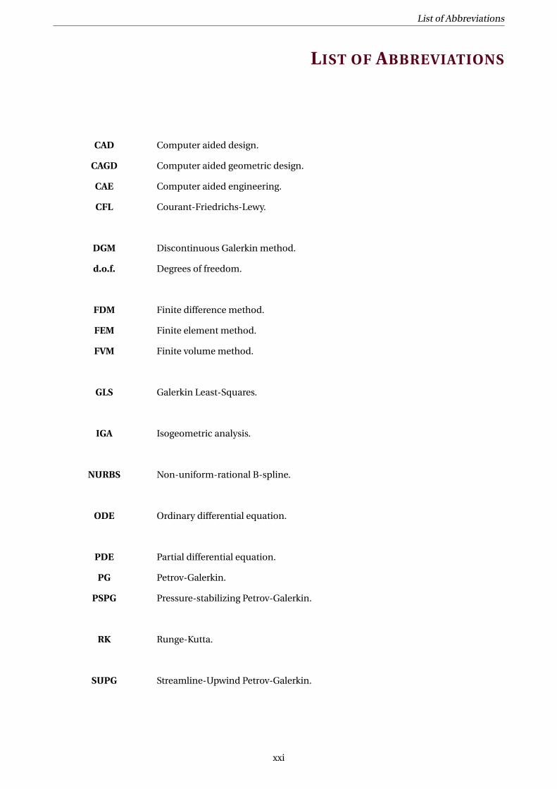
LIST OF ABBREVIATIONS
CAD Computer aided design.
CAGD Computer aided geometric design.
CAE Computer aided engineering.
CFL Courant-Friedrichs-Lewy.
DGM Discontinuous Galerkin method.
d.o.f. Degrees of freedom.
FDM Finite difference method.
FEM Finite element method.
FVM Finite volume method.
GLS Galerkin Least-Squares.
IGA Isogeometric analysis.
NURBS Non-uniform-rational B-spline.
ODE Ordinary differential equation.
PDE Partial differential equation.
PG Petrov-Galerkin.
PSPG Pressure-stabilizing Petrov-Galerkin.
RK Runge-Kutta.
SUPG Streamline-Upwind Petrov-Galerkin.
xxi

xxii

List of Symbols
LIST OF SYMBOLS
p Degree of the polynomial approximation.
n Number of B-spline functions of degree p.
nG Number of nodes for Gauss quadrature methods.
n Dimension of the time steps.
Nel Finite number of cells of DG method.
Nel Finite number of patchs of IGDG method.
N Dimension of the polynomial approximation.
B kp k-th Bernstein polynomial of degree p in parameter space.
Bkp k-th Bernstein polynomial of degree p in physical space.
Ni ,p i -th B-spline function of degree p in parameter space.
Ni ,p i -th B-spline function of degree p in physical space.
Rpi i -th NURBS function of degree p.
Cp Bézier curve of degree p.
Rp Rational Bézier curve of degree p.
S Bézier surface.
Cp B-spline curve of degree p.
S B-spline surface.
V B-spline volume.
Cp NURBS curve of degree p.
S NURBS surface.
Ξ Knot vector.
Ω Physical space.
∂Ω Boundary of the domainΩ.
Ω Parameter space.
Ω Reference element.
xxiii
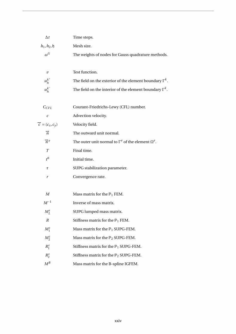
∆t Time steps.
h1,h2,h Mesh size.
ωG The weights of nodes for Gauss quadrature methods.
v Test function.
uk+h The field on the exterior of the element boundary Γk .
uk−h The field on the interior of the element boundary Γk .
CC F L Courant-Friedrichs-Lewy (CFL) number.
c Advection velocity.
−→c = (cx ,cy ) Velocity field.
−→n The outward unit normal.
−→n e The outer unit normal to Γe of the elementΩe .
T Final time.
t 0 Initial time.
τ SUPG stabilization parameter.
r Convergence rate.
M Mass matrix for the P1 FEM.
M−1 Inverse of mass matrix.
M sL SUPG lumped mass matrix.
R Stiffness matrix for the P1 FEM.
M s1 Mass matrix for the P1 SUPG-FEM.
M s2 Mass matrix for the P2 SUPG-FEM.
R s1 Stiffness matrix for the P1 SUPG-FEM.
R s2 Stiffness matrix for the P2 SUPG-FEM.
M B Mass matrix for the B-spline IGFEM.
xxiv

List of Symbols
(M B )T Transpose of the mass matrix for the B-spline IGFEM.
RB Stiffness matrix for the B-spline IGFEM.
Q The matrix defined by the least square method.
Mk Local mass matrix.
Rk Local stiffness matrix.
M k Local mass matrix for IGDGM.
Rk Local stiffness matrix for IGDGM.
J The Jacobian matrix.
| J | Determinant of the Jacobian.
J e The elemental Jacobian matrix in the physical domainΩe .
∂x u = ∂u∂x Partial derivative of u with respect to space x.
∂t u = ∂u∂t Partial derivative of u with respect to time t .
⊗ Tensor product.
C k The set of functions with k − th order continuous derivatives.
L Differential operator.
T Transformation of the parametric domain to the physical domain.
T−1 Inverse of transformation T.
Fe Numerical flux in the patchΩe .
fC E N Central flux.
fG Godunov flux.
fLF Lax-Friedrichs flux.
xxv


CH
AP
TE
R
1INTRODUCTION
HYperbolic systems of partial differential equations (PDEs) are mathematical mod-
els expressing the conservation of a physical quantity, as for instance mass, en-
ergy, etc. They arise naturally from the conservation laws in physics. In particular,
they describe a wide variety of phenomena that involve wave motion (such as acoustic, elastic, electromag-
netic) or the advective transport of substances.
The wide range of applications of hyperbolic PDEs led to a very intense research activity in this field. It al-
lowed to develop very early a set of numerical methods for accurate and computationally efficient approxi-
mations to the solutions of such problems. There are three major families of methods which are widely used:
the finite difference method, the finite volume method and the finite element method. These methods have
proved to be extremely useful in modeling a broad set of phenomena. To keep this thesis self-contained, we
briefly introduce each of these three methods in the context of hyperbolic PDEs.
Historically, the finite difference method (FDM) was the first method used to produce approximations
of the solutions of hyperbolic PDEs. They were introduced by Euler in the 18th century and represent the
easiest method to solve problems on simple geometries [64]. The main idea of this method, is to replace the
functional derivatives of the unknown by their FD approximations. The FDM is notable for the large variety
of schemes that can be used to approximate a given PDE; e.g. explicit schemes (Forward Euler, Upwind,
Lax-Friedrichs, Lax-Wendroff, Leapfrog, ...) and implicit schemes (Backward Euler, Crank-Nicolson,...) [88].
Although this method can be easily formulated and implemented, its application to problems with realis-
tic geometries is rather cumbersome, thus making the method not very attractive for industrial problems.
This fact urged the need for other methods with more flexibility, such as finite volume and finite element
methods.
1

CHAPTER 1. INTRODUCTION
The finite volume method (FVM) can handle complex geometries which makes it more attractive for
complex problems than the FDM. It is based on the conservative form instead of the differential form to
estimate the values of unknown fields. We split the domain into grid cells and approximate the total integral
over each grid cell, or actually the cell average, which is this integral divided by the volume of the cell. The
links between the cell quantities in the FVM rely on the flux between neighbouring control volumes. This
means that the FVM represents the flux of information within the structure of the mesh in a conservative
way [56]. It allows the use of unstructured grids to handle complex geometries.
The finite element method (FEM), had its origins in the early 1960s and is nowadays the predominating
method in analysis of elliptic or parabolic problems due to its flexibility to represent complex geometric
domains and its strong theoretical basis. The idea consists in decomposing the domain into many small,
“finite” elements which are defined by a set of nodal points and interpolating basis functions.
Although the FEM has been used widely in simulating many physical phenomena due to its flexibility to
represent complex geometric domains, it is well known in the FE literature that numerical difficulties arise
when solving hyperbolic PDEs. Indeed, when using the standard Galerkin FE method applied to hyperbolic
PDEs, unwanted spurious (non-physical) oscillations (Gibbs phenomenon) are frequently detected in the
numerical solutions. A cure to this drawback, widespread in the literature, is to add some "artificial" vis-
cosity to a standard (unstable) numerical scheme. On the one hand, this artificial viscosity should damp
the oscillations but, on the other hand, it should not smear the numerical solution. In the late 1970s and
early 1980s, a large number of so–called stabilized methods have been developed with different ideas [14]
[32] [48]. This is achieved through the use of a Petrov-Galerkin formulation [35], where the test functions
are modified such that they weight the upstream node more than the downstream node [17] [38]. Among
them, the most popular, so called Streamline-Upwind Petrov–Galerkin (SUPG) method, was introduced by
Brooks and Hughes. It was first proposed in the context of advection–diffusion equations and incompress-
ible Navier–Stokes equations [14], and then extended to various other problems, e.g., coupled multidimen-
sional advective–diffusive systems [44], first–order linear hyperbolic systems [49] or first–order hyperbolic
systems of conservation laws [45].
Later, Galerkin/least-squares (GLS) has emerged as a generalization of the SUPG method, developed by
Hughes et al. for convective transport problems [9] [30] [78], in which residuals of the equations in least-
squares form are added to the standard Galerkin formulation. GLS has been successfully employed in a wide
variety of applications where enhanced stability and accuracy properties are needed, including problems
governed by Navier-Stokes and the compressible Euler equations in fluid mechanics [78].
We can also mention the pressure-stabilizing/Petrov-Galerkin (PSPG) [91] formulation which has been in-
troduced for the stabilization of the Stokes equations [44] and incompressible Navier-Stokes equations [85].
2

The main idea of all these methods is to transform the original Galerkin method into a Petrov-Galerkin
formulation adapted to the physics considered. In fact, these formulations stabilize the method without in-
troducing excessive numerical dissipation. Because its symptoms are not necessarily qualitative, excessive
numerical dissipation is not always easy to detect. This concern makes it desirable to seek and employ stabi-
lized formulations developed with objectives that include keeping numerical dissipation to a minimum. In
these stabilized formulations, judicious selection of the stabilization parameter, which is almost known as
τ, plays an important role in determining the accuracy of the formulation. This yielded a significant amount
of attention and research [14] [30] [82] [83]. Typically this stabilization parameter involves a measure of the
local length scale (also known as "element length") and other parameters such as the local Reynolds and
Courant numbers. However, this stabilization parameter requires special attention, as it strongly depends
on the problem under consideration and the chosen numerical method.
More recently, an alternative approach has emerged, the discontinuous Galerkin method (DGM), which
shares some features with both the FVM and the FEM. Indeed, discontinuous polynomial functions are used
and a numerical flux is defined at the interface between cells to reconstruct the solution. It has been proved
very useful in solving a large range of problems. It was first introduced in 1973 by Reed and Hill for solving a
time-independent linear hyperbolic equations [74] and, later on, it has been extended for solving nonlinear
time-dependent equations. Subsequently, during the nineties of the last century the DGM experienced a
series of developments by Cockburn and Shu, where numerical schemes for hyperbolic problems were pro-
posed by combining DG approximation in space with Runge-Kutta time stepping strategies [18] [19] [21].
In fact, the DG method combines the advantages of stability of FVM and the accuracy of continuous FEM.
Within each element, the solution is approximated by a polynomial of degree p ≥ 0 (as in FEM), while the
continuity conditions applied to the solution are relaxed at the boundaries of elements (as in FVM), how-
ever, motivated by the FVM, interface terms of the problem are approximated by a consistent, monotone
and Lipschitz continuous numerical flux. This ensures that the scheme obtained is conservative, which
does not hold in case of the classical FEM. In particular, the increasing interest in these kind of formulations
are due to the following interesting features: they have good stability properties, they offer flexibility in the
mesh construction (irregular meshes are admissible) and in the handling of boundary conditions (Dirichlet
boundary conditions are weakly imposed), the accuracy is obtained by means of high-order polynomials
within elements, without any regularity constraint at element interfaces. Furthermore, they are locally con-
servative.
The fundamental difference between the DGM and the classical FEM relies on the continuity of basis
functions. In comparison with the classical FEM, in DGM the basis functions are completely discontinuous
across each element interface and they consist of local piecewise polynomials. Due to the fact that of basis
function have compact support, integration can be achieved locally in each element. This simplifies the
implementation of the method, since the mass matrix becomes block diagonal and the solution of a large
system is avoided. In addition, the discontinuity across each element allows the use of different degrees of
freedom in each element independently, which is not allowed in classical finite element method. Conse-
quently, we can easily apply adaptivity strategies by increasing the degrees of freedom near phenomena of
3
CHAPTER 1. INTRODUCTION
interest to obtain better approximations to the solution.
As explained above, FEM decomposes the computational domain into many small, “finite” elements
with simple shapes. A drawback is that with such elements there is usually no continuity higher than C 0 be-
tween elements. Even with higher-order polynomials it is difficult to guarantee C 1 continuity for arbitrarily
shaped elements. With the advancement in design technology a more accurate and flexible handling of the
geometry becomes necessary.
The design of free-from shapes by mathematical methods is a discipline, named computer-aided-design
(CAD). It had its origins slightly later than the computer-aided-engineering (CAE). In fact, CAD is the use of
computer technology for design: it allows the creation, modification, analysis and optimization of drawings
and geometric modeling. The Bézier curve was the first method used to construct free-form curves and
surfaces, and is named according to its inventor, Dr. Pierre Bézier. Bézier was an engineer in the Renault
car company and developed this method in 1966. Actually, another French engineer, Paul de Casteljau at
Citroën developed the same technology some years earlier. A further development to Bézier’s method were
B-splines which provide more flexibility in the modeling of free-form curves and surfaces. Since 1975 non-
uniform rational B-splines (NURBS) have been used in CAD programs, as a generalization of B-splines. The
development of NURBS provided a technology that can exactly describe circular shapes (cylinders, spheres,
etc.) which are basic elements in geometric modeling, but also allows very flexible modeling of free-form
surfaces [43].
Today, there is a strong need for reducing the gap between CAD and FEM in terms of geometric represen-
tations to gain in accuracy, flexibility and ease of interaction. A new form of analysis, named isogeometric
analysis (IGA), tries to close this gap between CAD and FEA in such a way that both disciplines work on the
same geometric models.
IGA is an extension of the FEM for solving PDEs. It was first introduced in 2005 by Hughes, Cottrell,
and Bazilevs [43], and expanded in 2006 [24] in an effort to bridge the gap between FEM and CAD. The key
idea is to use for analysis the same geometry used for geometric modeling. In fact, we use the same basis
functions, which are used for the representation of the geometry in computer aided design (CAD) mod-
els, also for the approximation of the solution of the PDE or the system of PDEs describing the physical
phenomenon. The idea of using Bézier, B-splines or NURBS as basis functions is driven by the desire to in-
tegrate CAD within FEM, and to have a strategy to replace a huge number of little cells (the FEs) by a reduced
set of larger patches covering the entire domain. Moreover, there are several advantages of this approach
over the FEM: easily control of the continuity, as C p−1-continuity is obtained using p-th order NURBS, ex-
act representation of the underlying NURBS geometry on the coarsest level of discretisation, as well as exact
representation of the geometry as the mesh is refined [43].
IGA has been applied to a wide variety of different physical phenomena, including computational solid
dynamics problems, computational fluid dynamics [23], coupled solid–fluid interaction problems [7] and
the diffusion equation [37]. In last years, there has been an increasing interest in DG-IGA for the numerical
solution of elliptic PDEs [40] [54] [69][95]. The advantages of the local approximation spaces without conti-
nuity requirements that DG methods offer [5] [28] is thus employed to manage multi-patch computations.
4
The main purpose of this thesis is to study the use of IGA to solve some hyperbolic problems. In par-
ticular, we describe the continuous and discontinuous Galerkin method using a B-spline basis. Special
emphasis is on the discontinuous Galerkin method, since it is considered as one of the most powerful and
fastest growing methods with applications in various problems, not necessarily hyperbolic. The disconti-
nuity of basis functions, which provides more flexibility in analysis, makes the method tedious however for
handling realistic geometries from CAD.
The thesis is structured in four main parts: the first gives particular focus on the Bernstein and B-splines
basis functions used in CAD. It is devoted to giving their definitions and basic properties. We present in the
second and third parts the extension from classical analysis to IGA for the FE and DG methods, for the one-
dimensional advection problem. In the last part, we deal with two dimensional hyperbolic problems by
combining the IGA with the DG method. It should be mentioned, in all this work, that the discretization of
equations in time is done by means of high-order explicit Runge-Kutta methods [18] [19] [34] [80].
More precisely, chapter 2 and chapter 3 provide a comprehensive introduction to the main ideas and
properties of the Bernstein, B-splines and NURBS, which form the basis for the IGA. In the same context,
an analysis of fitting B-spline curve and surface in the least squares sense is presented in chapter 4. The
analysis is illustrated by examples of univariate and bivariate problems. Since IGA is an extension of FEM,
we start by revisiting the original analysis framework in chapter 5, i.e. FEM. The need for stabilization is
outlined and stabilization ideas based on the Petrov-Galerkin concept are discussed. We focus on the SUPG
stabilization method and a special attention is given to the study of the stabilization parameter τ.
In chapter 6, the various computational procedures for IGA are reviewed in the context of FEM, by re-
visiting the one-dimensional advection problem that is given in the previous chapter. While in this chapter
we use B-splines (due to the simplicity of the domain) as a basis function, it is not hard to generalize it to
other splines such as NURBS. Detailed comparisons between both IGA and classical FEM are discussed.
In this context of IGA, we consider then the application of DG methods. Indeed, the major argument for us-
ing DG methods lies with their ability to provide stable numerical methods for hyperbolic PDE problems, for
which classical FEM is well known to perform poorly. Therefore, in chapter 7, we deal with one-dimensional
advection problem by combining IGA method with the DG method. We note that the DG methodology is
adopted at patch level, i.e., we employ the classical IGA within each patch, and employ the DG method
across the patch interfaces. Moreover, a transformation of the B-spline basis is necessary to introduce dis-
continuities at the interfaces, without modifying the geometry of the domain. The advantageous features
of both IGA and DG method enable us to design a promising formulation.
With some adjustments, chapter 8 and chapter 9 are devoted to the study of two numerical examples in
2D . The advection problem is first presented, followed by the acoustic wave equations, where both systems
are solved over several domains (Cartesian, linear and curvilinear).
Finally, in chapter 10 we end with some concluding remarks and outlooks. The results of the various
studies performed are summarized and discussed, and ideas for future research are proposed.
5


INTRODUCTION
LEs systèmes d’équations aux dérivées partielles (EDPs) hyperboliques sont des mod-
èles mathématiques permettant d’exprimer la conservation d’une quantité physique,
comme par exemple la masse, l’énergie, etc. Ils découlent naturellement des lois de
conservation en physique. En particulier, ils décrivent une grande variété de phénomènes impliquant le
mouvement des ondes (acoustiques, élastiques, électromagnétiques) ou le transport advectif de substances.
Le large éventail d’applications des EDPs hyperboliques a conduit à une activité de recherche très intense
dans ce domaine. Cela a permis de développer un ensemble de méthodes numériques pour des approxi-
mations précises et efficaces du point de vue du calcul des solutions à ces problèmes. Il existe trois grandes
familles de méthodes qui sont largement utilisées: la méthode des différences finies (MDF), la méthode des
volumes finis (MVF) et la méthode des éléments finis (MEF). Ces méthodes se sont révélées extrêmement
utiles pour modéliser un large éventail de phénomènes. Pour garder cette thèse autonome, nous présen-
tons brièvement chacune de ces trois méthodes dans le contexte des EDPs hyperboliques.
Historiquement, la méthode des différences finies (MDF) était la première méthode utilisée pour pro-
duire des approximations des solutions des EDPs hyperboliques. Elle a été introduite par Euler au 18ème
siècle et représente la méthode la plus simple pour résoudre des problèmes sur des géométries simples [64].
L’idée principale de cette méthode est de remplacer les dérivées partielles de l’inconnu par leurs approxi-
mations par des différences finis. La méthode DF est remarquable par la grande variété de schémas qui peu-
vent être utilisés pour approcher une EDP donnée, par exemples, schémas explicites (Forward Euler, Up-
wind, Lax-Friedrichs, Lax-Wendroff, Leapfrog, ...) et schémas implicites (Backward Euler, Crank-Nicolson,
...) [88]. Bien que cette méthode puisse être facilement formulée et mise en oeuvre, son application à des
problèmes avec des géométries réalistes est assez lourde, ce qui rend la méthode peu attrayante pour les
problèmes industriels. Cela a nécessité d’autres méthodes plus flexibles, telles que les méthodes de FV et
d’EF.
La méthode des VF peut gérer des géométries complexes ce qui la rend plus attrayante que la méthode
de DF pour les problèmes complexes. Elle est basée sur la forme conservative au lieu de la forme différen-
tielle pour estimer les valeurs des champs inconnus. On divise le domaine en cellules et on approxime
l’intégrale totale sur chaque cellule de la grille. Le liens entre les quantités de cellules dans la MVF dépen-
dent du flux entre les volumes de contrôle voisins. Cela signifie que la MVF représente le flux d’informations
dans la structure du maillage de manière conservative [56]. Elle permet l’utilisation de grilles non struc-
7

CHAPTER 1. INTRODUCTION
turées pour gérer des géométries complexes.
La méthode des éléments finis a ses origines au début des années 1960, elle est aujourd’hui la méth-
ode prédominante dans l’analyse des problèmes elliptiques ou paraboliques en raison de sa flexibilité à
représenter des domaines géométriques complexes et sa base théorique solide. L’idée consiste à décom-
poser le domaine en plusieurs éléments «finis», définis par un ensemble de points nodaux et des fonctions
de base interpolantes.
Bien que la MEF a été largement utilisée pour simuler de nombreux phénomènes physiques en raison
de sa flexibilité à représenter des domaines géométriques complexes, il est bien connu dans la littéra-
ture de la MEF que des difficultés numériques se posent lors de la résolution des EDPs hyperboliques.
En effet, lors de l’utilisation de la méthode d’EF standard appliquée à de tels EDPs, des oscillations para-
sites (non physiques) indésirables (phénomène de Gibbs) sont fréquemment détectées dans les solutions
numériques. Un remède à cet inconvénient, répandu dans la littérature, consiste à ajouter une viscosité "ar-
tificielle" à un schéma numérique standard (instable). D’une part, cette viscosité artificielle doit amortir les
oscillations mais, d’autre part, elle ne doit pas entacher la solution numérique. À la fin des années 1970 et au
début des années 1980, un grand nombre de méthodes dites stabilisées ont été développées avec des idées
différentes [14] [32] [48]. Ceci est réalisé grâce à l’utilisation d’une formulation Petrov-Galerkin [35], où les
fonctions test sont modifiées de telle sorte qu’elles pondèrent le noeud en amont plus que le noeud en aval
[17] [38]. Parmi eux, la plus populaire, dite Streamline-Upwind Petrov-Galerkin (SUPG), a été introduite
par Brooks et Hughes. Elle a été proposée d’abord dans le contexte des équations d’advection–diffusion
et les équations de Navier–Stokes incompressible [14], puis elle a été étendue à divers autres problèmes,
par exemples les systèmes advectifs–diffusifs multidimensionnels couplés [44], les systèmes hyperboliques
linéaires du premier ordre [49], les systèmes hyperboliques de lois de conservation [45].
Plus tard, la méthode de Galerkin/moindres carrés (GLS) est apparue comme une généralisation de la méth-
ode SUPG, développée par Hughes et al. pour les problèmes de transport convectif [9] [30] [78], dans laque-
lle les résidus des équations des moindres carrés sont ajoutés à la formulation de Galerkin standard. La
méthode GLS a été utilisée avec succès dans une large variété d’applications où des propriétés de stabilité
et de précision améliorées sont nécessaires, y compris les problèmes régis par Navier-Stokes et les équations
d’Euler compressible en mécanique des fluides [78]. On peut également citer la formulation de stabilisation
de la pression/Petrov-Galerkin (PSPG) [91] introduite pour la stabilisation des équations de Stokes [44] et
des équations de Navier-Stokes incompressibles [85].
8

L’idée principale de toutes ces méthodes est de transformer la méthode originale de Galerkin en une
formulation de Petrov-Galerkin adaptée à la physique considérée. En fait, ces formulations stabilisent le
procédé sans introduire de dissipation numérique excessive. Parce que les symptômes ne sont pas néces-
sairement qualitatifs, une dissipation numérique excessive n’est pas toujours facile à détecter. Cette préoc-
cupation rend la recherche et l’emploi de formulations stabilisées développées souhaitable avec des ob-
jectifs tels que le maintien au minimum de la dissipation numérique. Dans ces formulations stabilisées,
la sélection du paramètre de stabilisation, qui est souvent connu sous le nom de τ, joue un rôle impor-
tant dans la détermination de la précision de la formulation. Cela a suscité beaucoup d’attention et de
recherche [14] [30] [82] [83]. Ce paramètre de stabilisation implique généralement une mesure de l’échelle
de longueur locale (également appelée «longueur d’élément») et d’autres paramètres tels que les nombres
locaux de Reynolds et de Courant. Cependant, ce paramètre de stabilisation nécessite une attention parti-
culière, car il dépend fortement du problème considéré et de la méthode numérique stabilisée choisie.
Plus récemment, une approche alternative a émergé, la méthode de Galerkin discontinue (MGD), qui
partage certaines fonctionnalités avec MVF et MEF. En effet, des fonctions polynomiales discontinues sont
utilisées et un flux numérique est défini à l’interface entre les cellules pour reconstruire la solution. Elle s’est
avérée très efficace pour résoudre un large éventail de problèmes. Elle a été introduite pour la première fois
en 1973 par Reed et Hill pour résoudre des équations hyperboliques linéaires indépendantes du temps [74]
et plus tard, elle a été étendue pour résoudre des équations non linéaires dépendant du temps. Par la suite,
au cours des années quatre-vingt-dix du siècle dérnier, Cockburn et Shu ont développé une série de sché-
mas numériques pour les problèmes hyperboliques en combinant l’approximation de GD dans l’espace et
les stratégies de Runge-Kutta pour la discrétisation temporelle [18] [19] [21].
En fait, la méthode de GD combine les avantages de la stabilité de la MVF et la précision de la MEF continue.
Dans chaque élément, la solution est approchée par un polynôme de degré p ≥ 0 (comme dans la MEF),
tandis que les conditions de continuité appliquées à la solution sont relâchées aux limites des éléments
(comme dans la MVF), mais comme pour la MVF, les termes d’interface du problème sont approximés par
un flux numérique continu, monotone et Lipschitz. Cela garantit que le schéma obtenu est conservatif,
ce qui n’est pas le cas de la MEF classique. En particulier, l’intérêt croissant pour ce type de formulations
est dû aux caractéristiques intéressantes suivantes: elles ont de bonnes propriétés de stabilité, elles offrent
une flexibilité dans la construction du maillage (les maillages non structurés sont admissibles) et dans les
conditions aux limites (les conditions aux limites de Dirichlet sont faiblement imposées), la précision est
obtenue au moyen de polynômes d’ordre élevé dans les éléments, sans aucune contrainte de régularité aux
interfaces d’éléments.
La différence fondamentale entre la MGD et la MEF classique repose sur la continuité des fonctions
de base. En comparaison avec la MEF classique, dans la MGD, les fonctions de base sont complètement
discontinues pour chaque interface d’élément et elles sont constituées de polynômes locaux par élément.
Grâce au fait que des fonctions de base ont un support compact, l’intégration peut être réalisée localement
dans chaque élément. Cela simplifie la mise en oeuvre de la méthode, puisque la matrice de masse devient
diagonale en bloc et que la résolution d’un grand système est évitée.
9

CHAPTER 1. INTRODUCTION
De plus, la discontinuité entre chaque élément permet d’utiliser différents degrés de liberté dans chaque
élément indépendamment, ce qui n’est pas autorisé dans la méthode des EF classiques. Par conséquent,
nous pouvons facilement appliquer des stratégies d’adaptation en augmentant les degrés de liberté à prox-
imité de phénomènes d’intérêt pour obtenir de meilleures approximations de la solution.
Comme expliqué ci-dessus, la MEF décompose le domaine en plusieurs éléments «finis» avec des
formes simples. Un inconvénient est qu’avec de tels éléments, il n’y a généralement pas de continuité
supérieure à C 0 entre les éléments. Même avec des polynômes d’ordre supérieur, il est difficile de garantir
la continuité C 1 pour des éléments de forme arbitraire. Avec les progrès de la technologie de conception,
une manipulation plus précise et flexible devient nécessaire.
La conception de les formes libres par des méthodes mathématiques est une discipline appelée con-
ception assistée par ordinateur (CAO). Ses origines étaient un peu plus tardives que l’ingénierie assistée
par ordinateur (IAO). En fait, la CAO est l’utilisation de l’informatique pour la conception: elle permet la
création, la modification, l’analyse et l’optimisation de dessins et modélisations géométriques. Les courbes
de Bézier ont été la première méthode utilisée pour construire une forme libre des courbes et des surfaces,
elles sont nommées d’après leur inventeur Pierre Bézier. Bézier était ingénieur dans la société Renault au-
tomobile et a développé cette méthode en 1966 [?]. En fait, un autre ingénieur français, Paul de Casteljau
chez Citroën a développé la même technologie quelques années auparavant. Un autre développement de
la méthode de Bézier concerne les B-splines qui offrent plus de flexibilité dans la modélisation des courbes
et des surfaces de forme libre. Depuis 1975, les B-splines rationnelles non uniformes (NURBS) ont été util-
isées dans les programmes de CAO comme une généralisation de B-splines. Le développement de NURBS
a fourni une technologie capable de décrire exactement les formes circulaires (cylindres, sphères, etc.) qui
sont des éléments de base de la modélisation géométrique, mais permet également une modélisation très
flexible des surfaces à forme libre [43].
Aujourd’hui, il existe un fort besoin de réduire l’écart entre la CAO et la MEF en termes de représen-
tations géométriques pour gagner en flexibilité, précision et en facilité d’interaction. Une nouvelle forme
d’analyse, appelée analyse isogéométrique (AIG), tente de combler cet écart entre la CAO et la MEF de telle
manière que les deux disciplines fonctionnent avec les mêmes modèles géométriques.
L’AIG est une extension de la MEF pour la résolution des EDPs. Elle a été introduite pour la première fois en
2005 par Hughes, Cottrell et Bazilevs [43], et développé dans 2006 [24] pour tenter de combler le fossé entre
la MEF et la CAO.
10

L’idée principale est d’utiliser pour l’analyse la même géométrie utilisée pour la modélisation géométrique.
En fait, on utilise les mêmes fonctions de base, qui sont utilisées pour la représentation de la géométrie dans
les modèles de conception assistée par ordinateur (CAO), également pour l’approximation de la solution
des EDPs ou des systèmes des EDPs décrivant le phénomène physique. L’idée d’utiliser Bézier, B-splines
ou NURBS comme fonctions de base est motivée par le désir d’intégrer la CAO dans la MEF, et d’avoir une
stratégie pour remplacer un grand nombre de petites cellules (les EF) par un ensemble réduit de plus gros
patches couvrant tout le domaine. De plus, cette approche présente plusieurs avantages par rapport à la
MEF: contrôle facile de la continuité, car la continuité C p−1 est obtenue en utilisant une NURBS de degré p,
représentation exacte de la géométrie en utilisant une NURBS au niveau de discrétisation le plus grossier,
ainsi que la représentation exacte de la géométrie lorsque le maillage est affiné [43].
L’AIG a été appliquée à une grande variété de phénomènes physiques, y compris la dynamique des flu-
ides computationnelle [23], les problèmes d’interaction couplé fluide-structure [7] et l’équation de diffusion
[37]. Au cours des dernières années, la méthode de GD dans le cadre IG a manifesté un intérêt croissant pour
la solution numérique des EDPs elliptiques [40] [54] [69][95]. Les avantages des espaces d’approximation
locaux sans exigences de continuité offerts par les méthodes de GD [5] [28] sont alors utilisés pour gérer les
calculs multi-patch.
L’objectif principal de cette thèse est d’étudier l’utilisation des AIG pour résoudre certains problèmes
hyperboliques. En particulier, nous décrivons la méthode de Galerkin continue et discontinue en utilisant
la base des B-splines. Un accent particulier est mis sur la méthode de GD, car elle est considérée comme
l’une des méthodes les plus efficaces et à la croissance la plus rapide, avec des applications dans divers
problèmes, pas nécessairement hyperboliques. Les discontinuités des fonctions de base, qui offrent une
plus grande souplesse d’analyse, rendent cependant la méthode délicate pour gérer des géométries réal-
istes à partir de la CAO.
La thèse est divisée en quatre parties principales: la première met l’accent sur les fonctions de base de
Bernstein et B-splines utilisées en CAO. Elle est consacré à donner leurs définitions et propriétés de base.
Nous présenterons dans la deuxième et troisième parties l’extension de l’analyse classique à l’AIG pour
les méthodes d’EF et GD, pour le problème d’advection unidimensionnel. Dans la dernière partie, nous
traitons des problèmes hyperboliques en deux dimensions en combinant l’AIG avec la méthode de GD. Il
convient de mentionner que dans tout ce travail, la discrétisation des équations dans le temps se fait au
moyen de méthodes de Runge-Kutta explicites d’ordre élevé [18] [19] [34] [80].
Plus précisément, les deuxième et troisième chapitres fournissent une introduction complète aux prin-
cipales idées et propriétés des fonctions Bernstein, B-splines et NURBS, qui constituent la base de l’AIG.
Dans le même contexte, la construction des courbes B-spline et des surfaces au sens des moindres carrés
est présentée au quatrième chapitre. L’analyse est accompagnée d’exemples de problèmes univariés et bi-
variés.
11

CHAPTER 1. INTRODUCTION
L’AIG étant une extension de la MEF, nous commençons par revoir le cadre de l’analyse originale au cin-
quième chapitre, à savoir: la MEF. Le besoin de stabilisation est souligné et les idées de stabilisation basées
sur le concept Petrov-Galerkin sont discutés. Nous nous concentrons sur la méthode de stabilisation SUPG
et une attention particulière est accordée à l’étude du paramètre de stabilisation τ.
Au niveau du sixième chapitre, les différentes procédures de calcul pour l’AIG sont passées en revue
dans le contexte de la MEF, en revisitant le problème d’advection unidimensionnel qui est présenté dans le
chapitre précédent. Dans ce chapitre nous utilisons les B-splines (en raison de la simplicité du domaine)
comme fonctions de base, il n’est pas difficile de le généraliser pour d’autres splines telles que les NURBS.
Des comparaisons détaillées entre l’AIG et la MEF classiques sont discutées. Dans ce contexte de l’AIG, nous
considérons alors l’application des méthodes GD. En effet, l’argument majeur pour utiliser les méthodes
de GD réside dans leur capacité à fournir des méthodes numériques stables pour les EDPs hyperboliques,
pour lesquelles la MEF classique est bien connue pour ses performances médiocres. Par conséquent, au
septième chapitre, nous traitons le problème d’advection unidimensionnelle en combinant la méthode de
l’AIG avec la méthode de GD. Nous notons que la méthodologie de GD est adoptée au niveau du patch,
c’est-à-dire que nous employons l’AIG classique dans chaque patch et utilisons la méthode de GD à travers
les interfaces de patch. De plus, une transformation de la base B-spline est nécessaire pour introduire des
discontinuités aux interfaces, sans modifier la géométrie du domaine. Les caractéristiques avantageuses
des deux méthodes AIG et GD nous permettent de concevoir une formulation prometteuse.
Avec quelques ajustements, les huitième et neuvième chapitres sont consacrés à l’étude de deux ex-
emples numériques en 2D , le problème d’advection est d’abord présenté, suivi par les équations d’ondes
acoustiques, où les deux systèmes sont résolus sur plusieurs domaines (cartésien, linéaire et curviligne).
Enfin, au niveau du dernier chapitre, nous terminons avec quelques remarques et perspectives finales.
Les résultats des différentes études réalisées sont résumées et discutées et des idées de recherches futures
sont proposées.
12


Part I
CAD REPRESENTATIONS
14


CH
AP
TE
R
2BÉZIER CURVES
BÉzier curves are parametric curves commonly used in computer graphics and re-
lated fields. They are named after their inventor, Dr. Pierre Bézier, an engineer from
the Renault car company who developed in the early 1960′s a curve formulation for
use in shape design. The main interest of Bernstein-Bézier patches is that they lend to an easy geometric
understanding of the underlying mathematical concepts. Some basic properties and a brief discussion of
Bernstein polynomials and Bézier curves [8] are presented in the present chapter.
2.1 Bernstein basis
Bézier curves are expressed in terms of Bernstein polynomials which where introduced by Sergei Bern-
stein in order to formulate a constructive proof of the Weierstrass approximation theorem.
Definition 2.1.1. (Univariate Bernstein)
The Bernstein polynomials of degree p over the interval [0,1] are defined explicitly by:
B kp (ζ) =C k
pζk (1−ζ)p−k ∀ k = 0, ..., p,
with the binomial coefficients C kp given by:
C kp =
p !
k !(p−k)! if 0 ≤ k ≤ p,
0 otherwise.
16

2.1. BERNSTEIN BASIS
An example of constant, linear, quadratic and cubic Bernstein polynomials are presented in Fig. 2.1:
Figure 2.1: Constant, linear, quadratic and cubic Bernstein polynomials.
Definition 2.1.2. (Multivariate Bernstein)
In order to define Bernstein basis in higher dimensions, we make use of the tensor product construction. Let
p = (p1, p2, ..., pd ) be a vector inNd . The d-dimensional Bernstein polynomials are defined by a tensor product
of d univariate Bernstein polynomials with possibly different degrees p = (p1, p2, ..., pd ) and multi-indices
k = (k1,k2, ...,kd ).
Therefore, ∀ζ= (ζ1,ζ2, ...,ζd ) ∈ [0,1]d we get:
B kp (ζ) = B k1
p1(ζ1)⊗B k2
p2(ζ2)⊗ ...⊗B kd
pd(ζd ).
17

CHAPTER 2. BÉZIER CURVES
The bivariate Bernstein polynomials are illustrated in Fig. 2.2 for the linear, quadratic and cubic cases.
Figure 2.2: Linear, quadratic and cubic bivariate Bernstein polynomials.
18

2.2. PROPERTIES OF THE BERNSTEIN POLYNOMIALS
2.2 Properties of the Bernstein polynomials
The Bernstein polynomials B kp of degree p, have several important properties [50]:
1. Recursion
The Bernstein polynomials satisfy the following recursion relation: for p > 0, we have:B 0
p (ζ) = (1−ζ)p if k = 0,
B kp (ζ) = (
1−ζ)B kp−1(ζ)+ζB k−1
p−1(ζ) if k = 1, ..., p −1,
B pp (ζ) = ζp if k = p.
Proof.
∀1 ≤ k ≤ p −1, we have
(1−ζ)B k
p−1(ζ) = (1−ζ)C k
p−1ζk(
1−ζ)(p−1)−k
= C kp−1ζ
k(1−ζ)p−k
=(p −1
)!
k !((
p −1)−k
)!ζk(
1−ζ)p−k
=( p −k
p
)B k
p (ζ).
Similarly,
ξB k−1p−1(ζ) = ζC k−1
p−1ζk−1(1−ζ)(p−1)−(k−1)
= C k−1p−1ζ
k(1−ζ)p−k
=(p −1
)!(
k −1)!((
p −1)− (
k −1))
!ζk(
1−ζ)p−k
= ( k
p
)B k
p (ζ).
Therefore,
(1−ζ)B k
p−1(ζ)+ζB k−1p−1(ζ) = ( p −k
p
)B k
p (ζ)+ ( k
p
)B k
p (ζ)
= B kp (ζ).
19
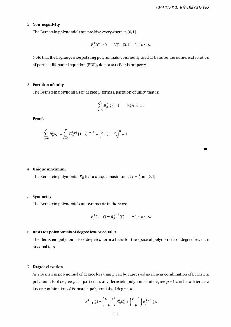
CHAPTER 2. BÉZIER CURVES
2. Non-negativity
The Bernstein polynomials are positive everywhere in [0,1].
B kp (ζ) ≥ 0 ∀ζ ∈ [0,1] 0 ≤ k ≤ p.
Note that the Lagrange interpolating polynomials, commonly used as basis for the numerical solution
of partial differential equation (PDE), do not satisfy this property.
3. Partition of unity
The Bernstein polynomials of degree p forms a partition of unity, that is:
p∑k=0
B kp (ζ) = 1 ∀ζ ∈ [0,1].
Proof.
p∑k=0
B kp (ζ) =
p∑k=0
C kpζ
k(1−ζ)p−k =
(ξ+ (1−ξ)
)p = 1.
4. Unique maximum
The Bernstein polynomial B kp has a unique maximum at ζ= k
p on [0,1].
5. Symmetry
The Bernstein polynomials are symmetric in the sens:
B kp (1−ζ) = B p−k
p (ζ) ∀0 ≤ k ≤ p.
6. Basis for polynomials of degree less or equal p
The Bernstein polynomials of degree p form a basis for the space of polynomials of degree less than
or equal to p.
7. Degree elevation
Any Bernstein polynomial of degree less than p can be expressed as a linear combination of Bernstein
polynomials of degree p. In particular, any Bernstein polynomial of degree p −1 can be written as a
linear combination of Bernstein polynomials of degree p.
B kp−1(ζ) =
(p −k
p
)B k
p (ζ)+(
k +1
p
)B k+1
p (ζ).
20

2.3. DERIVATIVES
Proof.(p −k
p
)B k
p (ζ)+(
k +1
p
)B k+1
p (ζ) =(
p −k
p
)C k
pζk(
1−ζ)p−k +(
k +1
p
)C k+1
p ζk+1(1−ζ)p−(k+1)
=(C k
pζk(
1−ζ)p−k)( p −k
p+
(k +1
p
)(p −k
k +1
)(ζ
1−ζ))
=(C k
pζk(
1−ζ)p−k)( p −k
p
)( 1
1−ζ)
= (p −1)!
k !(p −k −1)!ζk(
1−ζ)(p−1)−k
= B kp−1(ζ).
This property will play an important role, in the context of numerical solution of PDE, by allowing p-
refinement process.
2.3 Derivatives
The derivative of the k-th Bernstein polynomial of degree p is given by:
d
dζB k
p (ζ) = p(B k−1
p−1(ζ)−B kp−1(ζ)
).
Proof.
d
dζB k
p (ζ) = d
dζ
(C k
pζk(
1−ζ)p−k)
=C kp
(kζk−1(1−ζ)p−k − (
p −k)ζk(
1−ζ)p−k−1)
= k
ζ
(C k
pζk(
1−ζ)p−k)−
( p −k
1−ζ)(
C kpζ
k(1−ζ)p−k
)
= k
ζ
( p
kC k−1
p−1ζk(
1−ζ)p−k)−
( p −k
1−ζ)(
C kpζ
k(1−ζ)p−k
)
=(pC k−1
p−1ζk−1(1−ζ)p−k
)−
((p −k
)C k
pζk(
1−ζ)p−k−1)
=(pB k−1
p−1(ζ))−
((p −k
) p !
k !(p −k)!ζk(
1−ζ)p−k−1)
=(pB k−1
p−1(ζ))−
(p
(p −1)!
k !(p −k −1)!ζk(
1−ζ)p−k−1)
= pB k−1p−1(ζ)−pB k
p−1(ζ).
21

CHAPTER 2. BÉZIER CURVES
This formula is used to evaluate the derivatives of basis functions in the variational formulation, in a
recursive way.
2.4 Bézier curves
Definition 2.4.1. Given (p + 1) distinct points P0,P1, ...,Pp in space, the Bézier curve (of degree p) defined
from these points is the parametric curve Cp defined by:
Cp (ζ) =p∑
k=0B k
p (ζ)Pk ∀ζ ∈ [0,1].
The points(Pi
)i=0,...,p are called the control points and the line segments P0P1, P1P2, ..., Pp−1Pp form in this
order, the control polygon.
Figure 2.3: Bézier curves of various degrees and their control polygons.
Figure 2.3 depicts three different Bézier curves, with their corresponding control polygons. Each control
polygon is composed of its control points that are connected with line segments. Note that these control
polygons are not necessary closed.
2.5 Properties
Let us recall some important properties of a Bézier curve [46] [60], that will be useful for the numerical
solving PDE systems.
1. Interpolation at the extremities
A Bézier curve Cp of degree p, always starts at the first control point P0 and ends at last control point
Pp .
22

2.5. PROPERTIES
Figure 2.4: Bézier curves with endpoint interpolation.
This property is very important because, even if it is not necessary to fully control the curve in the
middle, it is essential to know where it starts and where it ends. If we want to connect several Bézier
curves, it is mandatory to know where the ends are. Moreover, this is important for applying Dirichlet
boundary conditions when solving PDE systems.
2. Invariance under affine transformation
An affine transformation of a Bézier curve is obtained by applying the transformation to the control
points.
Proof. Let ψ be an affine transformation in Rp :
ψ(X ) = AX +b with A ∈Mp (R) and b ∈Rp .
The affine transformation of a Bézier curve Cp of degree p is:
ψ(Cp (ζ)) = ψ( p∑
k=0B k
p (ζ)Pk
)= A
( p∑k=0
B kp (ζ)Pk
)+b
=p∑
k=0AB k
p (ζ)Pk +p∑
k=0bB k
p (ζ)
=p∑
k=0
(APk +b
)B k
p (ζ)
=p∑
k=0ψ(Pk )B k
p (ζ).
So ψ(Cp (ζ)) is a Bézier curve.
3. Convex hull
An important property of Bézier curves is that they always lies within the convex hull of their control
points. To explain this property we need to define the convex hull of a set of points.
23

CHAPTER 2. BÉZIER CURVES
Definition 2.5.1. (Convex hull)
The convex hull of a set P = P0,P1, ...,Pp of control points is the smallest convex polygon that contains
all the control points of P .
Figure 2.5: Cubic Bézier curve, its control polygon and the convex hull.
In Fig. 2.5, the convex hull of the 4 control points is shown. Again, this property can be exploited when
solving PDE, in particular in case of discontinuity capturing.
4. Local control
A Bézier curve is not interpolating the control points and moreover a Bézier curve changes globally
when a control point is modified.
An example for a quadric Bézier curve is presented in Fig. 2.6. The original curve is shown on the left. The
new Bézier curve after repositioning of the control point P2 is shown on the right. As we can see, the curve
is globally modified. This property can be a drawback and will justify the construction of B-spline curves
(see chapter 3).
Figure 2.6: Quadric Bézier curve and repositioning of the control point P2.
24
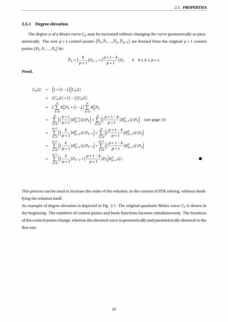
2.5. PROPERTIES
2.5.1 Degree elevation
The degree p of a Bézier curve Cp may be increased without changing the curve geometrically or para-
metrically. The new p + 2 control pointsP 0,P 1, ...,P p ,P p+1
are formed from the original p + 1 control
pointsP0,P1, ...,Pp
by:
P k = ( k
p +1
)Pk−1 +
( p +1−k
p +1
)Pk ∀ 0 ≤ k ≤ p +1.
Proof.
Cp (ζ) =(ζ+ (
1−ζ))Cp (ζ)
= ζCp (ζ)+ (1−ζ)Cp (ζ)
= ζp∑
k=0B k
p Pk +(1−ζ) p∑
k=0B k
p Pk
=p∑
k=0
(( k +1
p +1
)B k+1
p+1(ζ)Pk
)+
p∑k=0
(( p +1−k
p +1
)B k
p+1(ζ)Pk
)(see page 13)
=p+1∑k=1
(( k
p +1
)B k
p+1(ζ)Pk−1
)+
p∑k=0
(( p +1−k
p +1
)B k
p+1(ζ)Pk
)=
p+1∑k=0
(( k
p +1
)B k
p+1(ζ)Pk−1
)+
p+1∑k=0
(( p +1−k
p +1
)B k
p+1(ζ)Pk
)=
p+1∑k=0
(( k
p +1
)Pk−1 +
( p +1−k
p +1
)Pk
)B k
p+1(ζ).
This process can be used to increase the order of the solution, in the context of PDE solving, without modi-
fying the solution itself.
An example of degree elevation is depicted in Fig. 2.7. The original quadratic Bézier curve C2 is shown in
the beginning. The numbers of control points and basis functions increase simultaneously. The locations
of the control points change, whereas the elevated curve is geometrically and parametrically identical to the
first one.
25
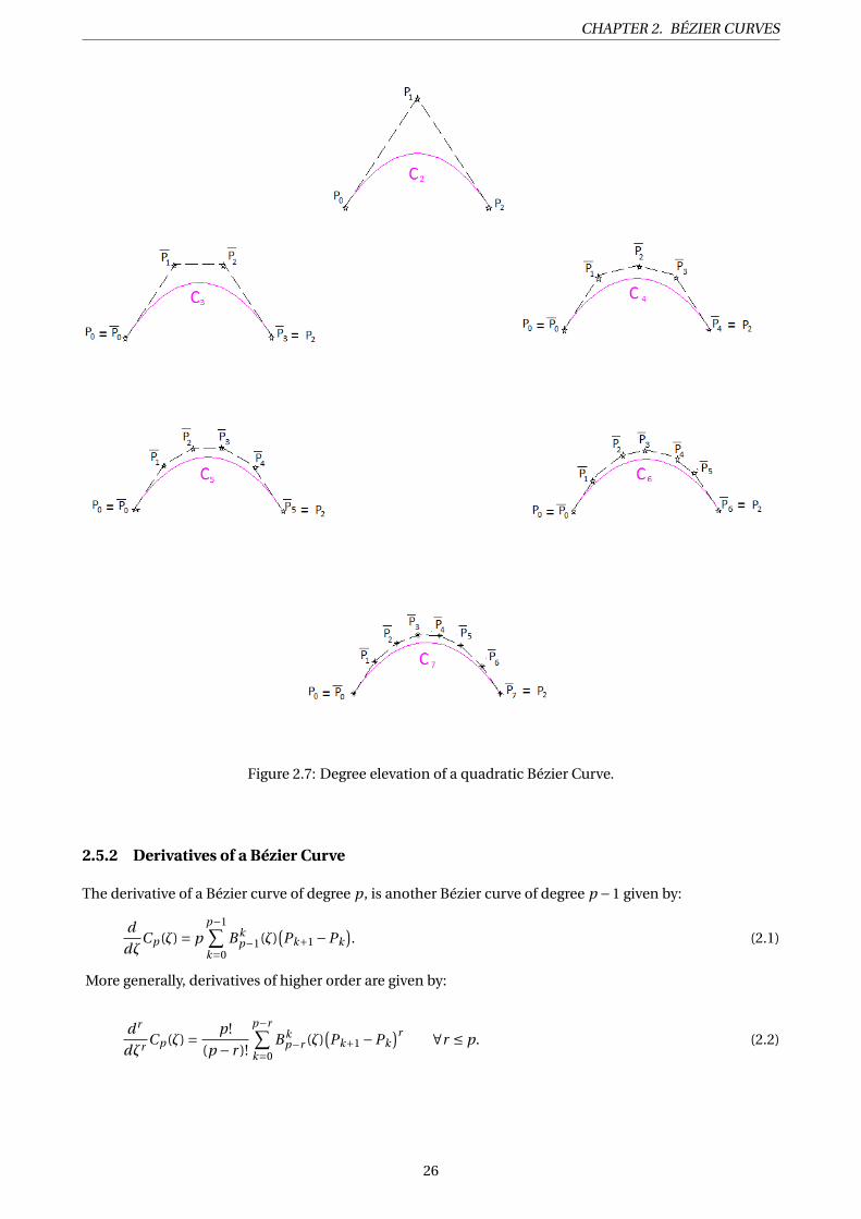
CHAPTER 2. BÉZIER CURVES
Figure 2.7: Degree elevation of a quadratic Bézier Curve.
2.5.2 Derivatives of a Bézier Curve
The derivative of a Bézier curve of degree p, is another Bézier curve of degree p −1 given by:
d
dζCp (ζ) = p
p−1∑k=0
B kp−1(ζ)
(Pk+1 −Pk
). (2.1)
More generally, derivatives of higher order are given by:
d r
dζr Cp (ζ) = p !
(p − r )!
p−r∑k=0
B kp−r (ζ)
(Pk+1 −Pk
)r ∀r ≤ p. (2.2)
26

2.5. PROPERTIES
This property has important consequences. In particular the curve at extremities is tangent to the first
and last control points lines. This could be used to apply Neumann boundary conditions for instance.
Proof.
For the first derivative, we have:
d
dζCp (ζ) = d
dζ
( p∑k=0
B kp (ζ)Pk
)=
p∑k=0
(dB kp (ζ)
dζ
)Pk
=p∑
k=0
(p(B k−1
p−1(ζ)−B kp−1(ζ))
)Pk
=(p
p∑k=0
B k−1p−1(ζ)Pk
)−
(p
p∑k=0
B kp−1(ζ)Pk
) (note that B−1
p−1(ζ) = B pp−1(ζ) = 0
)=
(p
p−1∑k=0
B kp−1(ζ)Pk+1
)−
(p
p−1∑k=0
B kp−1(ζ)Pk
)= p
p−1∑k=0
B kp−1(ζ)
(Pk+1 −Pk
).
This can be written as:
d
dζCp (ξ) = p
p−1∑k=0
B kp−1(ζ)Pk
= p !
(p −1)!
p−1∑k=0
B kp−1(ζ)Pk .
Now assume that (2.2) is true up to the order r . Let us prove it for r +1:
d r+1
dζr+1 Cp (ζ) = d
dζ
( d r
dζr Cp
)= d
dζ
( p !
(p − r )!
(p−r∑k=0
B kp−r (ζ)(Pk+1 −Pk )r
))= p !
(p − r )!
(p−r∑k=0
d
dζB k
p−r (ζ)(Pk+1 −Pk )r)
= p !
(p − r )!
(p−r∑k=0
((p − r )(B k−1
p−r−1(ζ)−B kp−r−1(ζ))
)(Pk+1 −Pk
)r+1)= p !
(p − r −1)!
(p−r∑k=0
(B k−1
p−r−1(ζ)−B kp−r−1(ζ)
)(Pk+1 −Pk
)r+1)= p !
(p − r −1)!
(p−r∑k=1
(Pk+1 −Pk )r+1B k−1p−r−1(ζ) −
p−r−1∑k=0
(Pk+1 −Pk )r+1B kp−r−1(ζ)
)= p !
(p − r −1)!
(p−r−1∑k=0
(Pk+1 −Pk )r+1B kp−r−1(ζ) −
p−r−1∑k=0
(Pk+1 −Pk )r+1B kp−r−1(ζ)
)= p !
(p − (r +1))!
(p−(r+1)∑k=0
(Pk+1 −Pk )r+1B kp−(r+1)(ζ)
).
Therefore, the result is true for (r +1).
27

CHAPTER 2. BÉZIER CURVES
2.6 Subdivision of Bézier curves
The De Casteljau algorithm is probably the most fundamental algorithm in the field of curve and surface
design. This algorithm was devised in 1959 by Paul De Casteljau, a French mathematician from the Citroen
automobile company. A main interest of this algorithm is to subdivide a Bézier curve Cp of degree p, de-
fined in [ζ1,ζl ], into two Bézier curves of degree p, C 1p defined in [ζ1,ζl 1 ] and C 2
p defined in [ζl 1 ,ζl ] whose
union is equivalent to the original curve.
Consider now a Bézier curve of degree p defined by the control points P0,P1, ...,Pp . The De Casteljau algo-
rithm is used to obtain a point on the curve at a parameter value ζ ∈ [0,1] from the control polygon com-
posed of the points Pi . We construct P ji : the new control point during the subdivision step j . Formally, the
algorithm of De Casteljau can be written as [65]:
P 0i = Pi i = 0, ..., p − r,
P ji = (1−ζ)P j−1
i +ζP j−1i+1 j = 1, ..., p i = 0, ..., p − j .
Fig. 2.8 illustrates the De Casteljau evaluation of a point on a cubic Bézier curve at ζ= 2/3. This algorithm
can also be represented as a triangular scheme, starting with four control points P0,P1,P2 and P3, and even-
tually reducing them to a single point P 30 .
Figure 2.8: Geometric construction according to De Casteljau’s algorithm for p = 3 and ζ= 2/3.
Thus, it is possible to subdivide a Bézier curve of degree p, into several curves which describe the same
curve. Because the resulting Bézier curves must have their own new control points, the original set of con-
trol points is discarded. Moreover, since the original Bézier curve Cp is cut into several pieces, each of which
is a subset of the original degree p Bézier curve, the resulting Bézier curves must be of degree p.
28

2.7. RATIONAL BÉZIER CURVES
Note that this algorithm is used in practice to evaluate the curve at a given parameter ζ (for visualization
for example).
2.7 Rational Bézier curves
Given (p+1) control points P0,P1, ...,Pp and associated nonnegative weights w0, w1, ..., wp we can define,
for ζ ∈ [0,1], the rational Bézier curve of degree p as:
Rp (ζ) =∑p
i=0 wi B ip (ζ)Pi∑p
i=0 wi B ip (ζ)
.
Note that if all weights are 1 (or if all weights are simply equal), a rational Bézier curve reduces to a poly-
nomial Bézier curve. However, almost all properties of Bézier curves still hold for rational Bézier curves
(details can be found in [29]). In particular, rational Bézier curves have end-point interpolation, prescribed
tangent lines at the endpoints. They also satisfy the convex hull property. Moreover, degree elevation and
subdivision can be extended to rational curves. Further, rational Bézier curves have several advantages over
polynomial Bézier curves. They provide more control over the shape than does a polynomial Bézier curve.
Elsewhere, it is possible to reparametrize the curve by simply changing the weights in a specific manner.
Moreover, rational Bézier curves are needed to exactly represent conic sections [55]. Therefore, their use is
fundamental in Computer-Aided-Design.
Fig. 2.9 shows several conic curves, which all share the same Bézier points, only the inner weight w changes.
Figure 2.9: Quadratic rational Bézier curves.
29

CHAPTER 2. BÉZIER CURVES
2.8 Bézier surface
One can easily extend the previous concepts to define Bézier surfaces, by using a second-order tensor
product of Bernstein polynomials. More precisely, a Bézier surface of degree p1 ×p2 can be formulated as:
S(ζ1,ζ2) =p1∑
i=0
p2∑j=0
B ip1
(ζ1)B jp2
(ζ2)Pi j ∀ζ1,ζ2 ∈ [0,1],
where the Pi j define a control net. The degrees of Bernstein polynomials p1 and p2 do not necessarily have
to be the same in the two parameter directions.
Fig. 2.10 gives an example of a tensor product Bézier surface of degree 3×3 and the corresponding control
net.
Figure 2.10: Tensor product Bézier patch of degree 3×3 and its control net.
The corresponding properties of the Bézier curve apply to the Bézier surface:
• Invariance under affine transformations.
• Subdivision produces smooth continuous surfaces.
• The Bézier surface is contained within the convex hull of the control nets.
• The Bézier surface can be exactly represented as a Bézier surface of higher degree.
• The Bézier surface does not in general pass through the control nets except for the corners of the control
net grid.
• Closed surfaces can be formed by setting the last control net equal to the first.
30


CONCLUSION
LEs courbes de Bézier ont été inventées dans les années 1960 par l’ingénieur Pierre
Bézier. Il a étudié le problème de conception de surfaces 3D (carrosseries d’automobiles,
fuselages d’avion, etc.) pour les premiers programmes de CAO (Conception Assistée
par Ordinateur). Le but était de trouver un moyen pour définir des courbes paramétriques de manière pré-
cise et simple.
Dans ce chapitre, nous avons examiné les polynômes de Bernstein et les courbes de Bézier détaillées dans
les deux cas, rationnel et non rationnel, et les surfaces par produits tensoriels ont été introduites. Diverses
exemples de courbes de Bézier ont été générées.
Nous avons discuté des propriétés des courbes de Bézier, ces propriétés sont directement impliquées dans
l’algorithme de Casteljau ou dans les propriétés des polynômes de Bernstein. Nous avons mentionné les
propriétés les plus fondamentales et nous avons fourni les preuves de ces propriétés brièvement.
En conclusion, nous avons vu que les courbes de Bézier ont un certain nombre de caractéristiques qui les
rendent intéressantes pour l’exploration du paramétrage géométrique. Ces courbes sont faciles à décrire
paramétriquement. Elles sont faciles à représenter graphiquement elles ont aussi l’avantage d’être incroy-
ablement pratiques, comme en témoigne leur utilisation dans la conception géométrique assistée par ordi-
nateur et infographie depuis les année 1960.
32


CH
AP
TE
R
3B-SPLINES CURVES
B-Spline and Non-Uniform-Rational B-spline (NURBS) (a generalization of B-spline)
are the de facto standard for geometric representation in computer aided design
(CAD) systems [43]. A brief discussion of B-spline and NURBS is presented in this
chapter. We begin by introducing necessary background concepts, defining commonly used notations and
introducing B-spline/NURBS curves and surfaces [23] [61] [75].
3.1 B-spline functions
Univariate B-spline functions are piecewise polynomial functions with compact support. They are de-
fined in parametric space using a so-called knot vector denotedΞ, in one-dimensional space (1D),Ξ is a set
of m non-decreasing coordinates:
Ξ= ξ1,ξ2, ...,ξm
.
Definition 3.1.1. The univariate B-spline function Ni ,p of degree p is defined according to the Cox–de Boor
recursion formula [27]:
For p = 0 :
Ni ,0(ξ) = 1 if ξi ≤ ξ< ξi+1 ∀i = 1, ...,m −1,
0 otherwise.(3.1)
34

3.1. B-SPLINE FUNCTIONS
For p ≥ 1:
Ni ,p (ξ) =( ξ−ξi
ξi+p −ξi
)Ni ,p−1(ξ)+
( ξi+p+1 −ξξi+p+1 −ξi+1
)Ni+1,p−1(ξ). (3.2)
Figure 3.1: Basis functions of degrees 1,2 and 3 for uniform knot vector Ξ= 0,1,2,3, ....
We use the convention that fraction in front of the basis functions is set equal to zero in the case of the
denominator being zero. That is:ξ−ξi
ξi+p −ξi≡ 0 if ξi+p −ξi = 0,
ξi+p+1 −ξξi+p+1 −ξi+1
≡ 0 if ξi+p+1 −ξi+1 = 0.
We see that there are exactly n basis functions. This is a direct consequence of the knot vector consisting of
n+p+1 knots. If we increase the number of elements in the knot vector, we will also increase the number of
basis functions. Note that the degree and the number of basis functions are independent, contrary to Bézier
functions.
With Eq. (3.1) and Eq. (3.2), it can be noted that for p = 0 and p = 1, the basis functions of isogeometric
analysis are identical to those of the standard piecewise constant and linear finite elements, respectively. In
fact, the greatest wealth of B-splines comes from the case p = 2.
35

CHAPTER 3. B-SPLINES CURVES
In order to define multivariate B-splines functions in higher dimensions, we make use of the tensor
product.
Definition 3.1.2. Let p = (p1, p2, ..., pd ) be a vector in Nd and for all j = 1, ...,d, let Ξ j be a 1D knot vector
defined by:
Ξ j =ξ
j1,ξ j
2, ...,ξ jn1+p1+1
.
Furthermore, if we denote the i j univariate B-spline of degree p j defined on the knot vector Ξ j by Ni j ,p j (ξ j ),
then, with the multi-indices i = (i1, i2, ..., id ), p = (p1, p2, ..., pd ) and n = (n1,n2, ...,nd ), the d-dimensional
tensor product B-spline is defined by:
Ni ,p (ξ) =Ni1,p1 (ξ1)⊗Ni2,p2 (ξ2)⊗ ...⊗Nid ,pd (ξd ).
Figure 3.2: Bivariates quadratic and cubic B-spline basis functions [16].
3.1.1 Knot Vectors
A knot vector Ξ in one-dimensional space is a set of finite, real-valued, monotonically increasing se-
quence of real numbers written,
Ξ= ξ1,ξ2, ...,ξn+p+1
,
where ξi ∈ R is the i − th knot, i ∈ 1,2, ...,n +p +1 is the knot index, p is the polynomial degree and n is
the number of basis functions which define the B-spline. The interval [ξ1, ...,ξi ] is called a patch ∀1 < i ≤n +p +1, whereas the interval between two knots [ξi ,ξi+1] is called knot span. A knot span is called empty
if ξi = ξi+1 and is called interior if ξi < ξi+1 ∀1 ≤ i ≤ n +p.
36

3.1. B-SPLINE FUNCTIONS
There are different types of knot vectors:
• Periodic knot vector: a knot vector Ξ is periodic if there exists an integer I and a real T such that for every
i ∈Z,
ξi+I = ξi +T.
• Uniform knot vector: if knots are equally-spaced in the parametric space, they are said to be uniform and
non-uniform otherwise.
• Open knot vetor: a knot vector for a B-spline basis of degree p is said to be open if the first and last knots
are repeated p +1 times.
Ξ= [ξ1, ...,ξ1︸ ︷︷ ︸
(p+1)times
,ξp+2, ...,ξn+p+1, ...,ξn+p+1︸ ︷︷ ︸(p+1)times
].
Open knot vectors are standard in the CAD literature. In one dimension, basis functions formed from open
knot vectors are interpolatory at the ends of the parametric space interval, [ξ1,ξn+p+1], and at the corners
of patches in multiple dimension but they are not, in general, interpolatory at interior knots. That is a dis-
tinguishing feature between "knots" and "nodes" in FEA.
The equations (3.1) and (3.2) show clearly that the choice of the knot vector has a significant influence on
the B-spline functions. An example of quadratic basis functions for an open, uniform knot vector is pre-
sented in Fig. 3.3.
Figure 3.3: Quadratic basis functions for the open-uniform knot vector Ξ= 0,0,0,1,2,3,3,3
.
37

CHAPTER 3. B-SPLINES CURVES
Note that the basis functions are interpolatory at the ends of the interval and also at ξ= 1, the location
of a repeated knot, where only C 0-continuity is attained (see Fig. 3.4).
Figure 3.4: Quadratic basis functions with reduced continuity at ξ= 1, Ξ= 0,0,0,1,1,2,3,3,3
.
In general, basis functions of degree p have p −1 continuous derivatives. If a knot is repeated k times (with
k < p), then the number of continuous derivatives decreases by k. When the multiplicity of a knot is exactly
p (i.e. k = p), the B-spline basis functions are C 0 continuous at that knot point. Obviously, if the multiplicity
of the knot point is p+1 (i.e. k = p+1) the B-spline basis functions are discontinuous at that knot point and
as a result two separate B-splines patches are formed.
This property will be used later, to generate a computational domain suitable to Discontinuous Galerkin
methods.
3.1.2 Properties of the B-spline functions
The B-spline functions Ni ,p defined using the procedure described above are polynomials of degree p.
There are several important features of the basis functions that are pointed out by Hughes et al. [23], in the
perspective of PDE analysis.
1. B-spline functions form a partition of unity, i.e.
n∑i=1
Ni ,p (ξ) = 1 ∀ξ ∈Ξ= ξ1,ξ2, ...,ξn+p+1
.
2. The basis functions are interpolatory at the end points of the knot vector, such that:
Ni ,p (ξ1) = δi ,1 and Ni ,p (ξn+p+1) = δi ,n
where, δ is the Kronecker symbol.
38

3.2. DERIVATIVES OF B-SPLINE FUNCTIONS
3. The support of each Ni ,p is compact and contained in [ξi ,ξi+p+1]. As seen in Fig. 3.4, the supports
of the functions are growing with increasing polynomial degree. In fact, the support will cover exactly
p + 2 knots. Note however that some of these knots may be equal and thus have knot multiplicity
greater than one. In these cases, the support will not go over p +1 knot spans, which is the maximum
support it can have.
4. Each B-spline function is nonnegative over the entire domain, that is:
Ni ,p (ξ) ≥ 0 ∀ξ ∈Ξ= ξ1,ξ2, ...,ξn+p+1
,
which means that all the coefficients of a mass matrix computed from a B-spline basis are also non-
negative, which can be useful for mass lumping schemes [23].
5. The B-spline functions indeed form a basis for the space of polynomials of degree less than or equal
to p, Pp . That is, they are all linearly independent i.e.
n∑i=1
αi Ni ,p (ξ) = 0 ⇐⇒ αi = 0 ∀i = 1,2, ...,n.
6. The B-spline function Ni ,p (ξi ) is of regularity C p−r at each knot of multiplicity r . When the multiplic-
ity of a knot is exactly p, the basis function is interpolatory.
3.2 Derivatives of B-spline functions
The derivatives of B-spline functions are represented in terms of lower order B-spline basis, as it comes
directly from the recursive definition given in equations (3.1) and (3.2). Thus, the first derivative of the i -th
B-spline basis function of degree p is given by:
d
dξNi ,p (ξ) = p
(( 1
ξi+p −ξi
)Ni ,p−1(ξ)− ( 1
ξi+p+1 −ξi+1
)Ni+1,p−1(ξ)
). (3.3)
Proof. ddξNi ,0(ξ) = 0
(Ni ,0(ξ) and Ni+1,0(ξ) are constants
).
d
dξNi ,1(ξ) = d
dξ
(( ξ−ξi
ξi+1 −ξi
)Ni ,0(ξ)+ ( ξi+2 −ξ
ξi+2 −ξi+1
)Ni+1,0
)=
( 1
ξi+1 −ξi
)Ni ,0(ξ) −
( 1
ξi+2 −ξi+1
)Ni+1,0.
39

CHAPTER 3. B-SPLINES CURVES
We assume that for all 0 ≤ q ≤ p, we have:
dNi ,q (ξ)
dξ=
( q
ξi+q −ξi
)Ni ,q−1(ξ) −
( q
ξi+q+1 −ξi+1
)Ni+1,q−1(ξ).
Let us prove that (3.3) is true for p +1.
d
dξNi ,p+1(ξ) = d
dξ
(( ξ−ξi
ξi+p+1 −ξi
)Ni ,p (ξ)+ ( ξi+p+2 −ξ
ξi+p+2 −ξi+1
)Ni+1,p (ξ)
)
=( 1
ξi+p+1 −ξi
)Ni ,p (ξ)+
( ξ−ξi
ξi+p+1 −ξi
)(dNi ,p (ξ)
dξ
)−
( 1
ξi+p+2 −ξi+1
)Ni+1,p (ξ)
+( ξi+p+2 −ξξi+p+2 −ξi+1
)(dNi+1,p (ξ)
dξ
)
=( 1
ξi+p+1 −ξi
)Ni ,p (ξ) +
( ξ−ξi
ξi+p+1 −ξi
)(( p
ξi+p −ξi
)Ni ,p−1(ξ)− ( p
ξi+p+1 −ξi+1
)Ni+1,p−1(ξ)
)
−( 1
ξi+p+2 −ξi+1
)Ni+1,p (ξ)+
( ξi+p+2 −ξξi+p+2 −ξi+1
)(( p
ξi+p+1 −ξi+1
)Ni+1,p−1(ξ)− ( p
ξi+p+2 −ξi+2
)Ni+2,p−1(ξ)
)
=( 1
ξi+p+1 −ξi
)Ni ,p (ξ) +
( p
ξi+p −ξi
)( ξ−ξi
ξi+p+1 −ξi
)Ni ,p−1(ξ) −
( 1
ξi+p+2 −ξi+1
)Ni+1,p (ξ)
+(( −p
ξi+p+1 −ξi+1
)( ξ−ξi
ξi+p+1 −ξi
)+ ( p
ξi+p+1 −ξi+1
)( ξi+p+2 −ξξi+p+2 −ξi+1
))Ni+1,p−1(ξ)
+( −p
ξi+p+2 −ξi+2
)( ξi+p+2 −ξξi+p+2 −ξi+1
)Ni+2,p−1(ξ).
( p
ξi+p+1 −ξi+1
)(( ξi+p+2 −ξξi+p+2 −ξi+1
)− ( ξ−ξi
ξi+p+1 −ξi
))Ni+1,p−1 =
( p
ξi+p+1 −ξi+1
)( ξi+p+2 −ξξi+p+2 −ξi+1
− ξi+p+2 −ξi+1
ξi+p+2 −ξi+1
)Ni+1,p−1
+( p
ξi+p+1 −ξi+1
)(ξi+p+1 −ξi
ξi+p+1 −ξi− ξ−ξi
ξi+p+1 −ξi
)Ni+1,p−1
=( p
ξi+p+1 −ξi+1
)( ξi+1 −ξξi+p+2 −ξi+1
+ ξi+p+1 −ξξi+p+1 −ξi
)Ni+1,p−1.
40

3.3. B-SPLINE CURVES
Then, we get:
d
dξNi ,p+1(ξ) =
( 1
ξi+p+1 −ξi
)Ni ,p (ξ) −
( 1
ξi+p+2 −ξi+1
)Ni+1,p (ξ) +
( p
ξi+p+1 −ξi
)( ξ−ξi
ξi+p −ξiNi ,p−1(ξ)
+( ξi+p+1 −ξξi+p+1 −ξi+1
)Ni+1,p−1(ξ)
)+
( p
ξi+p+1 −ξi+1
)( ξi+1 −ξξi+p+2 −ξi+1
)Ni+1,p−1(ξ)
+( −p
ξi+p+2 −ξi+2
)( ξi+p+2 −ξξi+p+2 −ξi+1
)Ni+2,p−1(ξ)
=( p +1
ξi+p+1 −ξi
)Ni ,p (ξ)−
( 1
ξi+p+2 −ξi+1
)Ni+1,p (ξ)
+( −p
ξi+p+2 −ξi+1
)( ξ−ξi+1
ξi+p+1 −ξi+1Ni+1,p−1(ξ) + ξi+p+2 −ξ
ξi+p+2 −ξi+2Ni+2,p−1(ξ)
)
=( p +1
ξi+p+1 −ξi
)Ni ,p (ξ) −
( p +1
ξi+p+2 −ξi+1
)Ni+1,p (ξ).
3.3 B-spline curves
B-spline curves are defined as a linear combination of control points and B-spline basis functions.
Given n basis functions Ni ,p , i = 1, ...,n and corresponding control points Pi ∈ R, i = 1, ...,n, a piecewise-
polynomial B-spline curve is obtained as:
Cp (ξ) =n∑
i=1Ni ,p (ξ)Pi .
The linear interpolation of the control points is called the control polygon. It can be seen that a Bézier curve
of order n + 1 (degree n) is a special case of B-spline curve with no internal knots and the ends knots are
repeated n +1 times. The knot vector is thus:
Ξ= 0,0, ...,0︸ ︷︷ ︸
(n+1)t i mes
, 1,1, ...,1︸ ︷︷ ︸(n+1)t i mes
.
An example is shown in Fig. 3.5 for the quadratic basis functions considered previously. Note that the curve
is interpolatory at the first and last control points P1 and P5, due to the fact that the knot vector is uniform
and open, Ξ= 0,0,0,1,2,3,3,3
. The curve C2 is tangent to the control polygon at the first and last control
points. The curve is C 1 continuous everywhere.
41

CHAPTER 3. B-SPLINES CURVES
Figure 3.5: Quadratic B-spline curve.
B-spline curves are generalization of Bézier curves and share many important properties with them. More-
over, B-spline curves have additional useful properties [23]. We list below some of the most important prop-
erties of B-spline curves:
• The curve Cp is C p−1 continuous everywhere except at the knot or control point of multiplicity r , where it
is C p−r .
• Invariance with respect to affine transformations. In fact, an affine transformation of a B-spline curve is
obtained by applying the transformation directly to the control points.
• If the knot vector is open, the curve starts at the point P1 and ends at Pn . Moreover, it is tangent to (P0P1)
and (Pn−1Pn) at the extremities.
• Changing the position of control point Pi affects Cp only in the interval [ξi ,ξi+p ], which is a significant
difference with respect to Bézier curves.
Figure 3.6: A quadratic B-spline curve and its control points. In the right, the curve after moving the controlpoint P4.
42

3.4. HIERARCHICAL REPRESENTATION
• B-spline curve is contained in the convex hull of its control point. More specifically, if ξ ∈ [ξi ,ξi+1), then
Cp (ξ) is in the convex hull of control points Pi−p ,Pi−p+1, ...,Pi .
• The derivative of a B-spline curve is given by:
d
dξCp (ξ) = p
(n−1∑i=0
( Pi+1 −Pi
ξi+p+1 −ξi+1
))Ni+1,p−1(ξ).
3.4 Hierarchical representation
The B-spline curves can be enriched by three types of refinements, which are termed h−, p− and k−refinements, without changing the shape of the geometry. For further details, we refer the reader to [23].
3.4.1 Knot insertion
The first mechanism by which one can enrich the basis is knot insertion. Knots may be inserted without
changing a curve geometrically or parametrically. More precisely, given a B-spline curve with m control
points Pi , the same curve can be obtained with m +1 control points Pi by inserting ξ ∈ [ξk ,ξk+1[ given by:
Pi =αi Pi + (1−αi )Pi−1,
where,
αi =
1 if i ≤ k −p,ξ−ξi
ξi+p−ξiif k −p +1 ≤ i ≤ k,
0 if i ≥ k +1.
An example of knot insertion is presented in Fig. 3.7.
Figure 3.7: Before and after knot insertion (cubic B-spline curve).
43

CHAPTER 3. B-SPLINES CURVES
The original curve, shown on the left, consists of a cubic B-spline curve with 9 control points and has
9+3+1 = 13 knot values. The new curve, shown on the right, is geometrically and parametrically identical
to the first one, but the basis functions and control points are changed, there is one more of each. This
process may be repeated to enrich the solution space by adding more basis functions of the same order
while keeping the curve unchanged. Insertion of new knot values clearly has similarities with the classical
h−refinement strategy in FEA. As explained in section 3.1.1, inserting a knot on an existing knot results in a
decrease of the curve regularity (multiple knots).
3.4.2 Order elevation
The second mechanism by which one can enrich the basis is order elevation (sometimes also called
“degree elevation”) can be thought of as p−refinement in FEA. During this process, the multiplicity of each
knot is increased by one but no new knots are added. Let Ξ = ξ1, ...,ξm be a knot vector, the degree p
of a B-spline curve Cp defined for the knot vector Ξ may be increased without changing the geometry or
parametrization. It is possible to define another B-spline curve of degree p+1 that is identical to the original
one. The number of new control points depends on the multiplicities of existing knots. The process for order
elevation is the following:
1. Begins by subdividing the curve into many Bézier curves of degree p by knot insertion (see section
3.7).
2. The next step is to elevate the order of the polynomial on each of these individual segments (see
section 2.5.1).
3. Last, excess knots are removed to combine the segments into a B-spline curve of degree p +1.
The basic idea of degree raising and knot insertion is to achieve the flexibility without changing the shape
of the curve or surface. We refer to [23] for the mathematical details.
3.4.3 k−refinement
k−refinement refers to the process in which order elevation is followed by knot insertion. It has no
analogous in FEA. It is important to point out that the order elevation and knot insertion do not commute.
This process results in a higher order and higher continuity basis than the process of knot insertion followed
by order elevation. We refer to [23] for a thorough treatment and application examples.
44

3.5. B-SPLINE SURFACES AND VOLUMES
3.5 B-spline surfaces and volumes
Given a control net (Pi , j )i=1,...,n j=1,...,m and two knot vectors,Ξ1 = ξ1, ...,ξn+p+1 andΞ2 = η1, ...,ηm+q+1,
a tensor-product B-spline surface is defined as:
S (ξ,η) =n∑
i=1
m∑j=1
Ni ,p (ξ)N j ,q (η)Pi , j .
Figure 3.8: B-spline surface example.
B-spline volumes are defined using a third-order tensor product of B-spline functions. Given a control
net Pi , j ,k , i = 1, ...,n, j = 1, ...,m, k = 1, ...,r and knot vectors Ξ1 = ξ1, ...,ξn+p+1, Ξ2 = η1, ...,ηm+q+1 and
Ξ3 = ζ1, ...,ζl+l+1, a B-spline volume is defined by:
V (ξ,η,ζ) =n∑
i=1
m∑j=1
l∑k=1
Ni ,p (ξ)N j ,q (η)Nk,r (ζ)Pi , j ,k .
It is important to note that many properties of a B-spline surface and volume are the results of the tensor
product nature. Multivariate B-splines basis functions are nonnegative, have local support, are invariant to
affine transformations and form a partition of unity.
45

CHAPTER 3. B-SPLINES CURVES
3.6 Non-Uniform Rational B-spline (NURBS)
B-splines are convenient for free-form modelling, but they lack the ability to exactly represent some
simple shapes such as circles and ellipsoids. NURBS are non-rational functions of B-splines, they allow for
the exact parametrization of common curves and surfaces such as circles, cylinders and spheres. They are
also extremely flexible and intuitive when dealing with more complex shape creation and deformation. A
NURBS entity in Rd is obtained by the projective transformation of a B-spline entity in Rd+1 [23].
3.6.1 NURBS basis functions
Let (wi )1≤i≤n be a sequence of non-negative reals (weights for control point). The i -th NURBS function
of degree p, associated to the knot vector Ξ and the weights w , is given by:
Rpi (ξ) = Ni ,p (ξ)wi∑n
j=1 N j ,p (ξ)w j,
where Ni ,p (ξ) denotes the i -th B-spline basis function of degree p.
The first derivative of a NURBS basis function is given by:
d
dξR
pi (ξ) = wi
ddξNi ,p (ξ)W (ξ)−Ni ,p (ξ) d
dξW (ξ)
W 2(ξ),
where,
W (ξ) =n∑
j=1N j ,p (ξ)w j ,
d
dξW (ξ) =
n∑j=1
d
dξN j ,p (ξ)w j .
3.6.2 NURBS curves and surfaces
The NURBS curve of degree p associated to the knot vector Ξ, the control points (Bi )1≤i≤n and the
weights (wi )1≤i≤n is defined as:
Cp (ξ) =n∑
i=1R
pi (ξ)Bi .
Similarly, the NURBS surfaces of degree p1 ×p2 associated to the knot vectors Ξ1 and Ξ2, the control nets
(Bi , j )1≤i≤n1,1≤ j≤n2 and the weights (wi j )1≤i≤n1,1≤ j≤n2 , are defined by:
S(ξ,η) =n1∑
i=1
n2∑j=1
Ri j (ξ,η)Bi , j .
With,
Ri j (ξ,η) = wi j Ni ,p1 (ξ)N j ,p2 (η)∑n1i=1
∑n2j=1 wi j Ni ,p1 (ξ)N j ,p2 (η)
46

3.7. EXTRACTING BÉZIER CURVES FROM B-SPLINES
We recall some important properties of NURBS (we refer to [23] for more details):
• NURBS basis functions forms a partition of unity.
• The continuity and support of NURBS basis functions are the same as for B-splines.
• Affine transformations in physical space are obtained by applying the transformation to the control
points, that is, NURBS possess the property of affine invariance.
• If the weights are equal, NURBS become B-splines.
• NURBS surfaces and solids are the projective transformations of tensor product, piecewise polyno-
mial entities.
3.7 Extracting Bézier curves from B-splines
Let us consider the knot vector Ξ= ξ1, ...,ξn+p+1
where, ξ1 = ... = ξp+1 and ξn+1 = ξn+p+1.
To decompose a B-spline (or NURBS) curve to its Bézier elements, called Bézier extraction, a straightforward
approach consists in using the knot-insertion procedure several times, for each of the existing interior knots
(ξp+2, ...,ξn) until interior knots have a multiplicity p + 1. Then, the original B-spline curve is separated
in independant Bézier elements. The curve is geometrically unmodified, but its representation is split in
a set of discontinuous elements. This is the key procedure to build a computational domain suitable to
Discontinuous Galerkin method.
It is important to point out that the Bézier patch is a particular case of B-spline patch, for which the number
n of functions (and control points) is equal to p+1. An example illustrating Bézier extraction from quadratic
B-spline is shown in Fig. 3.9.
47

CHAPTER 3. B-SPLINES CURVES
Figure 3.9: Bézier decomposition (bottom) from a quadratic B-spline basis (top) by knot insertion.
48


CONCLUSION
LEs courbes B-splines ont été définies dans les années 1970 par Cox et DeBoor, pour
remédier à l’inconvénient de la globalité des courbes de Bézier, à travers un algo-
rithme efficace car hiérarchique (analogue à celui de Casteljau), stable numérique-
ment (coefficients multiplicatifs toujours positifs) et interprétable géométriquement: le déplacement d’un
point de contrôle de la courbe n’affecte ainsi plus qu’une partie limitée de la courbe, ce qui amène un plus
grand confort dans la Conception Assistée par Ordinateur (CAO).
Par conséquent, les courbes B-splines permettent d’approcher des points de manière lisse, comme les
coubes de Bézier. Leur avantage est qu’elles sont plus lisses et plus faciles à contrôler.
Dans ce chapitre, nous avons présenté des définitions formelles des fonctions et des courbes B-splines,
ainsi qu’une étude détaillée des propriétés les plus fondamentales des B-splines, illustrées par des exemples
et des figures.
50


CH
AP
TE
R
4CURVE AND SURFACE FITTING
CUrve or surface fitting, also known as regression analysis, is used to approximate a
curve or surface for a series of data points. Most of the time, the curve/surface fitting
is used to find points and derivatives anywhere along the curve/surface. This proce-
dure is attractive because of its ability to produce an interpolating curve/surface that retains extremely high
accuracy with a minimal number of data to represent the curve/surface, so that the error is minimized in
the least squares sense. The purpose of this chapter is to present the problem of fitting a given ordered set
of data with a B-spline curve or surface in the least squares sense.
In the context of isogeometric analysis, this technique will be used in the following two cases:
• to define the B-spline computational domain if the geometry of the problem is not defined originally in
terms of B-spline,
• to define the B-spline initial conditions.
4.1 Curve fitting
4.1.1 Basic concepts
Curve or surface fitting is a fundamental problem in many fields, such as computer graphics, image
processing, shape modeling and data mining. Depending on applications, different types of curves such
as parametric curves, implicit curves and subdivision curves are used for fitting [53] [96]. In this chapter,
we discuss the problem of B-spline curve and surface fitting [10] [57]. Due to the fact that the curve and
surface fitting are closely related topics, we define and discuss the curve fitting problem first and show how
to generalize it to surface reconstructions later on.
52

4.1. CURVE FITTING
The general objective of curve fitting is to theoretically describe experimental data with a model (func-
tion or equation) and to find the parameters associated with this model.
We recall that a B-spline curve of degree p is defined for a collection of n control points (Pi )i=1,...,n by:
Cp (ξ) =n∑
i=1Ni ,p (ξ)Pi .
The functions Ni ,p (ξ) are the B-spline basis functions of degree p, which are defined recursively and require
the selection of a sequence of scalars ξi ∈Ξ= ξ1,ξ2, ...,ξn+p+1
.
Let (ζk )1≤k≤neval such that ζ1 < ζ2 < ... < ζneval and let Q be a set of ordered and distinct points Qk , ∀k =1, ..,neval to be fitted.
The basic aim is to fit a B-spline curve that will approximate neval measured data points in a least squares
sense (with neval À n). This leads to find an optimal set of control point Pi 1≤i≤n producing an optimal
approximating B-spline Cp with minimal distances to the points Qk . We seek therefore to minimize the
least-squares error, defined as the sum of squares of the points distance expressed as:
1
2
neval∑k=1
∣∣∣ n∑i=1
Ni ,p (ζk )Pi −Qk
∣∣∣2,
where∑n
i=1 Ni ,p (ζk )Pi is the B-spline curve point at ζk and Qk is the corresponding measured data point.
4.1.2 Description of the least squares method
The least-squares estimation procedure is a mathematical tool that was developed independently by
Carl Friedrich Gauss in 1795 and Adrien-Marie Legendre who published it first in 1805 [52]. This theory
describes a frequently used approach evolved from statistical methods to estimate values of parameters of
a mathematical model from measured data, which are subject to errors.
For a specified set of control points, the least-squares error function between the B-spline curve and sample
points is the scalar-valued function:
E(P ) = 1
2
neval∑k=1
∣∣∣ n∑j=1
N j ,p (ζk )P j −Qk
∣∣∣2. (4.1)
As it has been pointed previously, the goal is to find values of the control points that minimize the error.
Therefore, we find the values of Pi 1≤i≤n in such a way that:
∂E
∂Pi= 0.
53

CHAPTER 4. CURVE AND SURFACE FITTING
Thus, carrying out the differentiation leads to:
∂E
∂Pi= ∂
∂Pi
(1
2
neval∑k=1
∣∣∣ n∑j=1
N j ,p (ζk )P j −Qk
∣∣∣2)=
neval∑k=1
( n∑j=1
N j ,p (ζk )P j −Qk
)Ni ,p (ζk )
=neval∑k=1
n∑j=1
Ni ,p (ζk )N j ,p (ζk )P j −neval∑k=1
Ni ,p (ζk )Qk
=neval∑k=1
n∑j=1
aki ak j P j −neval∑k=1
aki Qk ,
where aki =Ni ,p (ζk ).
Setting the partial derivatives equal to the zero vector (0Rn ) leads to the system of equations:
0Rn =neval∑k=1
n∑j=1
aki ak j P j −neval∑k=1
aki Qk
= At AP − AtQ,
where a matrix A ∈Rneval×n given by: A = (aki
)1≤k≤neval ,1≤i≤n .
This system of equations is a least-squares formulation for an over determined problem.
Hence, the minimization leads to the linear system:
At AP = AtQ. (4.2)
As consequence, the equation 4.2 is equivalent to solving:
P = (At A
)−1 AtQ. (4.3)
4.2 B-spline curve fitting - example
In this section, an example of Least-squares B-spline curve fitting is given to illustrate the performance
of the method.
Consider the sinusoidal function:
f (x) = sin(2πx) ∀x ∈Ω= [−1,1].
In our example we consider fitting a data set of neval uniformly distributed parameters (ζk )1≤k≤neval and
points Qk = sin(2πζk ), ∀1 ≤ k ≤ neval . In this case, we choose neval = 80 À n = 8. As seen in Fig. 4.1 an
accurate approximation is obtained using only 8 control points.
54

4.3. LEAST-SQUARES B-SPLINE SURFACE FITTING
Figure 4.1: The least-squares quadratic B-spline curve fitting.
4.3 Least-squares B-spline surface fitting
A B-spline tensor product surface is defined for a bi-dimensional array of n ×m control points Pi j with
1 ≤ i ≤ n and 1 ≤ j ≤ m,
S (ξ,η) =n∑
i=1
m∑j=1
Ni ,p (ξ)N j ,q (η)Pi , j . (4.4)
The numbers p and q are the degrees for the surface, Ni ,p (ξ) and N j ,q (η) are the B-spline basis functions.
The sample data points are (ζk1 ,θk2 ,Qk1k2 ) with 1 ≤ k1 ≤ neval and 1 ≤ k2 ≤ meval . It is assumed that:
ζ1 < ζ2 < · · · < ζneval and θ1 < θ2 < · · · < θmeval .
The control points may be arranged formally as an n ×m matrix.
P =
P11 · · · P1m
.... . .
...
Pn1 · · · Pnm
.
Similarly, the samples Qk1k2 may be arranged formally as an neval ×meval matrix:
Q =
Q11 · · · Q1meval
.... . .
...
Pneval 1 · · · Pneval meval
.
55

CHAPTER 4. CURVE AND SURFACE FITTING
For a specified set of control points, the least-squares error function between the B-spline surface and
sample points is the scalar-valued function:
E(P ) = 1
2
neval∑k1=1
meval∑k2=1
∣∣∣ n∑j1=1
m∑j2=1
N j1,p (ζk1 )N j2,q (θk2 )P j1 j2 −Qk1k2
∣∣∣2. (4.5)
We determine as previously the control points by minimizing the error function.
The first-order partial derivatives are written in terms of the control points P j1 j2 rather than in terms of the
components of the control points:
∂E
∂Pi1i2
= ∂
∂Pi1i2
(1
2
neval∑k1=1
meval∑k2=1
∣∣∣ n∑j1=1
m∑j2=1
N j1,p (ζk1 )N j2,q (θk2 )P j1 j2 −Qk1k2
∣∣∣2)
=neval∑k1=1
meval∑k2=1
( n∑j1=1
m∑j2=1
N j1,p (ζk1 )N j2,q (θk2 )P j1 j2 −Qk1k2
)Ni1,p (ζk1 )Ni2,q (θk2 )
=neval∑k1=1
meval∑k2=1
n∑j1=1
m∑j2=1
N j1,p (ζk1 )N j2,q (θk2 )Ni1,p (ζk1 )Ni2,q (θk2 )P j1 j2
−neval∑k1=1
meval∑k2=1
Ni1,p (ζk1 )Ni2,q (θk2 )Qk1k2
=neval∑k1=1
meval∑k2=1
n∑j1=1
m∑j2=1
ak1 j1 bk2 j2 ak1i1 bk2i2 P j1 j2 −neval∑k1=1
meval∑k2=1
ak1i1 bk2i2Qk1k2 ,
where ak1 j1 =N j1,p (ζk1 ) and bk2 j2 =N j2,q (θk2 ).
These equations may be written in matrix notation as:
∂E
∂P= At APB t B − AtQB , (4.6)
where, A = (ak j
)1≤k≤neval ,1≤ j≤n is a neval ×n matrix, and B = (
bk j)
1≤k≤meval ,1≤ j≤m is a meval ×m matrix.
Setting the partial derivatives equal to the zero matrix 0Rn×m leads to the matrix system of equations,
At APB t B − AtQB = 0Rn×m . (4.7)
Then, we get:
P =((
At A)−1 At
)Q
(B
(B t B
)−1)
=((
At A)−1 At
)Q
((B t B
)−1B t)t
.
56

4.4. B-SPLINE SURFACE FITTING - EXAMPLES
4.4 B-spline surface fitting - examples
Figures 4.2 and 4.5 show two examples of least squares quadratic B-spline fitting surfaces. These two
cases will be used in forthcoming chapters for isogeometric analysis applications. Note that the least-
squares fitting method presented previously is applied patch by patch when the computational domain
is composed by a set of patches.
The first example is the two-dimensional Gaussian function.
f (x, y) = a exp(−
( (x −x0)2
2σ2x
+ (y − y0)2
2σ2y
))∀(x, y) ∈Ω= [−1,1]× [−1,1].
Here the coefficient a is the amplitude, x0, y0 is the center and σ2x ,σ2
y are the x and y spreads of the blob.
Figure 4.2 created using a = 1, (x0, y0) = (0,0), and σx =σy = 1/p
2.
The physical domain Ω is a set of quadratic Bézier patch with 5×5 patches. The mesh type considered is a
simple Cartesian grid. In each patch, we define local data points (ζk1 ,θk2 ,Qk1k2 ) ∀1 ≤ k1 ≤ neval ,1 ≤ k2 ≤meval , with neval = meval = 30.
Figure 4.2: The least-squares quadratic B-spline Gaussian surface fitting.
The second example is the Bessel functions of the first kind.
Bessel equation (named according to the astronomer Friedrich Wilhelm Bessel) is a second-order differen-
tial equation with two linearly independent solutions: a Bessel function of the first kind of order ν, Jν and a
Bessel function of the second kind of order ν, Yν, where ν is a non-negative real number. We refer the reader
to [25].
57

CHAPTER 4. CURVE AND SURFACE FITTING
The Bessel function of the first kind Jν(x) can be written as an infinite polynomial:
Jν(x) =∞∑
i=0
(−1)i
i !Γ(ν+ i +1)
( x
2
)ν+2i ,
where Γ is the gamma function, satisfy: Γ(i ) = (i −1)! for i a positive integer.
Some Bessel functions are plotted in Fig. 4.3.
Figure 4.3: Bessel functions of the first kind-1D .
In our example, we consider a fitting a data set of neval = 30 points and meval = 30 points taken from a
part of the disc defined by(x(r,θ), y(r,θ)
), for 0.25 ≤ r ≤ 1 and 0 ≤ θ ≤ π
2 . The computational domain Ω is
defined as a set of quadratic Bézier patches with 8×8 patches. The mesh type considered in this example
is curvilinear and approximates the geometrical domain. The function to be fitted is defined in cylindrical
coordinates as Jν(r ).
Figure 4.4: Representation of the physical domainΩ.
58

4.4. B-SPLINE SURFACE FITTING - EXAMPLES
B-spline fitting curves can be seen in Fig. 4.5, for 8×8 quadratic patches.
Figure 4.5: The least-squares quadratic B-spline surface fitting.
59


CONCLUSION
L’ajustement des courbes et des surfaces est un problème fondamental dans de nom-
breux domaines, tels que l’infographie, le traitement d’images, la modélisation de
formes et l’exploration de données. Selon les applications, différents types de courbes,
telles que les courbes paramétriques, les courbes implicites et les courbes de subdivision, sont utilisées pour
ajuster. Dans ce chapitre, nous avons discuté le problème de l’ajustement de courbes et surfaces B-splines
en se basant sur l’approximation par moindres carrés.
La méthode d’approximation par moindres carrés est un outil mathématique, développé indépendamment
par Carl Friedrich Gauss en 1795 et Adrien-Marie Legendre qui l’a publié en 1805. Cette théorie décrit une
approche fréquemment utilisée à partir de méthodes statistiques pour estimer les valeurs des paramètres
d’un modèle mathématique à partir de données mesurées, qui sont sujettes à des erreurs.
Dans le cadre de l’analyse isogéométrique, cette technique est utilisée dans deux cas suivants:
• pour définir le domaine de calcul B-spline si la géométrie du problème n’est pas définie à l’origine en ter-
mes de B-spline,
• pour définir les conditions initiales dans l’espace de représentation B-spline.
61


Part II
ISOGEOMETRIC ANALYSIS - FINITE
ELEMENT FRAMEWORK (ILLUSTRATION
FOR A 1D PROBLEM)
63


CH
AP
TE
R
5SUPG - FINITE ELEMENT METHOD
THe aim of IGA is to generalize and improve upon classical FEA. In this chapter, we start by
giving an introduction to IGA by revisiting the original analysis, i.e. FEA, in the context
of hyperbolic PDEs.
The stabilized method Streamline Upwind/Petrov Galerkin (SUPG) [14] [48] [63] had its origin in the late
1970s and early 1980s. In the present chapter, the capability of this stabilized Finite Element Method (FEM)
is illustrated by means of the linear advection problem. A special attention is given to the identification of
the stabilization parameter τ of this method which weights the stabilization terms. The need for stabiliza-
tion is outlined and the basic idea of the Petrov-Galerkin (PG) concept are discussed.
5.1 Preliminaries
For the arguments to follow we would like to introduce some notations and definitions.
The first space we need is the space of square-integrable functions L2(Ω) defined by:
L2(Ω) =
u |∫Ω| u |2 dΩ<∞
where Ω an open internal of R.
There is a norm related to this space, denoted by ∥ . ∥L2(Ω) which is defined by:
∥ u ∥L2(Ω)=(∫Ω
u2dΩ) 1
2.
We also will need one of the wide family of Sobolev spaces H 1(Ω) which is defined by:
H 1(Ω) =
u ∈ L2(Ω) such thatdu
d x∈ L2(Ω)
.
H 1(Ω) is a Hilbert space with inner product
(v, w)1,Ω =∫Ω
v(x)w(x)d x +∫Ω
v ′(x)w ′(x)d x,
65

CHAPTER 5. SUPG - FINITE ELEMENT METHOD
and the associated norm:
∥ v ∥1,Ω=∥ v ∥2L2(Ω) + ∥ v ′ ∥2
L2(Ω) .
5.2 Standard Galerkin FEM
Given a one-dimensional domain Ω =]a,b[, we consider the one-dimensional hyperbolic model prob-
lem of a scalar conservation law, with boundary and initial conditions, which can be written as:
∂u(x,t )∂t + ∂
∂x f (u(x, t )) = 0 ∀(x, t ) ∈]a,b[×[0,T ],
u(x,0) = u0(x) ∀x ∈]a,b[,
u(a, t ) = ua(t ) ∀t ∈ [0,T ],
(5.1)
where u denotes an unknown scalar variable, while f (u) is called flux function and ∂u∂t indicates the partial
derivative of u with respect to time t , and t 0 = 0 indicates initial time. In addition, we represent by ∂u∂x the
partial derivative of u with respect to space.
The classical variational approach associated with (5.1) is obtained by multiplying this equation by a test
function v supposed to be sufficiently regular and by integrating over the domainΩ. We denote by V 1 such
space of functions, verifying the boundary conditions:
V 1 =
w ∈ H 1(Ω) such that w(a) = ua
.
We introduce the space H 1([0,T ],V 1) of functions v : from [0,T ] to V 1, such that ∂v∂t ∈ L2([0,T ]).
The weak form of the state equation (5.1) is given by: Find u ∈ H 1([0,T ],V 1) such that:∫Ω
∂u(x, t )
∂tv(x)d x +
∫Ω
∂
∂xf (u(x, t ))v(x)d x = 0 ∀t ∈ [0,T ] ∀v ∈ H 1(Ω). (5.2)
By integrating by parts and using Dirichlet boundary conditions, the variational formulation reads:
Find u ∈ H 1([0,T ],V 1) such that:∫Ω
∂u(x, t )
∂tv(x)d x =
∫Ω
f (u(x, t ))v ′(x)d x + f (ua)v(a)− f (ub)v(b) ∀v ∈ H 1(Ω). (5.3)
As consequence, the weak formulation of the problem (5.1) may be rewritten as: Find u ∈ H 1([0,T ],V 1) such that :
a(u, v) = L(v) ∀v ∈ H 1(Ω),(5.4)
where,
a(u, v) =∫Ω
∂u(x, t )
∂tv(x)d x −
∫Ω
f (u(x, t ))v ′(x)d x,
and
L(v) = f (ua)v(a)− f (ub)v(b).
66

5.3. LAGRANGE P1 ELEMENTS
5.3 Lagrange P1 elements
We first consider a mesh of the 1D computational domain Ω =]a,b[, where we want to compute the
solution. A mesh is simply a set of points (xi )1≤i≤N or intervalsΩi = [xi , xi+1], ∀1 ≤ i ≤ N −1 such that:
a = x1 < x2 < ... < xN = b.
Figure 5.1: Uniform P1 mesh of [a,b].
The mesh is said to be uniform if the points (xi )1≤i≤N are uniformly distributed along the segment [a,b].
The cell size or space step is defined by h1 = b−aN−1 , where N −1 is the number of cells in the mesh. The coor-
dinates of the grid points are then defined by xi+1 = x1 + i h1, ∀1 ≤ i ≤ N −1.
The FEM for Lagrange P1 elements involves the space of globally continuous affine functions on each inter-
val:
V 1h =
wh ∈C 0(Ω) wh |Ωi
∈P1(Ωi ),∀i = 1,2, ..., N −1 such that wh(a) = ua
,
V 1h is a subspace of V 1 of dimension N . Moreover, every function uh ∈V 1
h is uniquely determined by:
uh(x, t ) =N∑
j=1uh(x j , t )ϕ j (x) ∀x ∈Ω,
where ∀2 ≤ j ≤ N −1, ϕ j is the basis of the shape functions defined as:
ϕ j (x) =
x−x j−1
h1if x ∈ [x j−1, x j ],
x j+1−xh1
if x ∈ [x j , x j+1],
0 otherwise.
These functions are shown in Fig. 5.2. Their construction involves satisfies:
ϕ j (xi ) = δi j ∀i , j = 1, ..., N .
67

CHAPTER 5. SUPG - FINITE ELEMENT METHOD
Figure 5.2: Global shape functions for the space V 1h .
By choosing the test functions vh equal to the basis functions of V 1h , one obtains:
Find uh ∈V 1h such that for all i = 1, ..., N ,
N∑j=1
∂u j (t )
∂t
∫Ωϕi (x)ϕ j (x)d x =
∫Ω
f (uh(x, t ))ϕ′i (x)d x + f (ua)ϕi (a)− f (ub)ϕi (b) ∀t ∈ [0,T ]. (5.5)
Now we rewrite equation (5.1) with Ω =]−1,1[ and f (u(x, t )) = cu(x, t ) such that c > 0 is the advection ve-
locity. For simplicity in what follows, we assume c to be constant.
Let us consider the problem:
∂u(x,t )∂t + c ∂u(x,t )
∂x = 0 ∀(x, t ) ∈]−1,1[×[0,T ],
u(x,0) = u0(x) = sin(2πx) ∀x ∈]−1,1[,
u(−1, t ) = ua(t ) ∀t ∈ [0,T ],
(5.6)
where,
ua(t ) = sin(2π(−1− ct )). (5.7)
Note that no boundary condition is prescribed at x = 1 due to the hyperbolicity of the problem.
The exact solution to this problem is:
uex (x, t ) = u0(x − ct ) = sin(2π(x − ct )).
68

5.3. LAGRANGE P1 ELEMENTS
We present in Fig. 5.3 the exact solution of the problem (5.6) for a transport speed c = 1.
Figure 5.3: The exact sine wave solution for the one-dimensional advection problem.
Thus, we get the discrete weak formulation given by: Find u1(t ) = uh(x1, t ), ...,uN (t ) = uh(xN , t ) such that
for all i = 1, ..., N
N∑j=1
∂u j (t )
∂t
∫Ωϕi (x)ϕ j (x)d x = c
N∑j=1
u j (t )∫Ωϕ j (x)ϕ′
i (x)d x + cuaϕi (a)− cu(b)ϕi (b) ∀t ∈ [0,T ], (5.8)
which can be rewritten in the form of linear system:
M∂tU = RU + cUa − cUb, (5.9)
where U (t ) is the vector whose components are u j (t ), the unknown values at the grid point at time t, M and
R are the mass and stiffness matrices whose coefficients are:
Mi j =∫Ωϕi (x)ϕ j (x)d x ∀i , j = 1, ..., N ,
Ri j = c∫Ωϕ′
i (x)ϕ j (x)d x ∀i , j = 1, ..., N ,
and
U =
u1
...
uN
∈RN , Ua =
sin(2π(−1− ct ))
0...
0
∈RN , Ub =
0
0...
uN
∈RN .
69

CHAPTER 5. SUPG - FINITE ELEMENT METHOD
In the FEM, the matrices M and R are computed from the corresponding elementary matrices which
are obtained by applying a local change of variables to map each cellΩ onto the reference element.
After integration, we get:
M = h1
6
2 1 0 · · · · · · 0
1 4 1 0 · · · 0. . .
. . .. . .
. . .. . .
. . .
. . .. . .
. . .. . .
. . .. . .
0 · · · 0 1 4 1
0 0 · · · 0 1 2
and R = c
2
1 −1 0 · · · · · · 0
1 0 −1 0 · · · 0. . .
. . .. . .
. . .. . .
. . .
. . .. . .
. . .. . .
. . .. . .
0 · · · 0 1 0 −1
0 · · · 0 0 1 1
.
Therefore, the semi-discrete formulation in space is given by: ∀2 ≤ i ≤ N −1,
h1
6
(∂t ui−1 +4∂t ui +∂t ui+1
)+ c(ui+1 −ui−1
2
),
where, ui−1, ui and ui+1 are the values of u at nodes i −1, i and i +1 respectively.
We can conclude that classical Galerkin FEM has similarities with the use of central differenciation in the
Finite Difference Method (FDM) for the advection problem for which the advection term writes c Ui+1−Ui−12
(identical to −RU ).
The coefficients ui are time-dependent while the basis and test functions depend just on spatial co-
ordinates. Further, the time derivative is not discretized in the time domain. One approach would be to
use FEM for the time domain as well, but this can be rather computationally expensive. Alternatively, an
independent discretization of the time domain is often applied using the method of lines. For example, it is
possible to use the explicit Euler scheme:
Given the initial value problem:∂U (x,t )∂t = L
(t ,U (x, t )
),
U (x, t 0) = U0(x),(5.10)
we approximate the partial differential equation (5.10) by the finite-difference formulation:
U (x, t +∆t )−U (x, t )
∆t=L
(t ,U (x, t )
).
This is exactly one step of the explicit Euler method. Introducing the notation: t n+1 = t n +∆t ,
U n =U (t n),
we have,
U n+1 =U n +∆tL(t n ,U n)
.
70

5.3. LAGRANGE P1 ELEMENTS
Euler explicit method is employed to integrate the equations in time with the timestep ∆t chosen small
enough to ensure that time discretization errors can be neglected. Assuming that M is invertible, we have:
U n+1 = U n +∆t M−1RU n + c∆t M−1(U na −U n
b
). (5.11)
This example demonstrates the limitations of the standard Galerkin method for solving advection problem,
we observe in Fig. 5.4 that the approximate solution of the problem oscillates.
Figure 5.4: Exact and standard Galerkin FEM P1 solution for the one-dimensional linear advection problemat T = 0.4s.
Therefore, standard Galerkin FEM applied to these problems is far from "optimal" and gives unphysical os-
cillatory solutions, well known as Gibbs phenomena [14]. The attenuation of these oscillations has been the
subject of extensive research for several decades during which a huge number of so–called stabilized meth-
ods have been developed. The stabilizing effect can be often interpreted as the addition of some artificial
diffusion to a standard (unstable) numerical scheme. On the one hand, this artificial diffusion should damp
down the oscillations. On the other hand, it should not smear the numerical solution so that the design of a
proper stabilization is a very difficult task.
71

CHAPTER 5. SUPG - FINITE ELEMENT METHOD
In the late 1970s and early 1980s, a number of methods have been proposed to remove or, at least, to
diminish these oscillations (a good summary of the very early literature is contained in [14] [32] [48]). Thus,
the attention of FE researchers was turned to the development of Petrov-Galerkin methods (PGM), which
are based on searching the test functions that provide exact nodal values for a selected class of solutions.
Using these test functions in the general case induces a stabilizing effect which removes the wiggles ob-
tained with the classical Galerkin method [63]. In the context of FEM, there are several approaches, among
the most popular techniques, we can name the so called Streamline-Upwind Petrov-Galerkin (SUPG)[13]
[84], Galerkin Least-Squares (GLS) [9] [30] [78] and Pressure-Stabilizing Petrov-Galerkin (PSPG) [91]. All
these methods are based on a PG FEM. The main idea of all these methods is to add products of suitable
perturbation terms and the residuals, thereby maintaining consistency. In these stabilized formulations, a
judicious selection of the stabilization parameter, which is often denoted as τ, plays an important role in
determining the accuracy of the formulation [1] [15]. This stabilization parameter requires special atten-
tion, as it strongly depends on the problem under consideration and the chosen numerical method.
We here give a brief outline of the theoretical basis for PG FEM. Given a differential operator L and a func-
tion G , we consider the problem:
L u(x) =G(x) ∀x ∈Ω, (5.12)
whereΩ⊂R (without loss of generality on Rd ). The weak form of (5.12) is given by:∫Ω
(L u −G)v∗dΩ= 0.
The problem is discretised based on the following formula:
u =N∑
j=1u jϕ j , (5.13)
where ϕ j 1≤ j≤N are mesh-based shape functions.
Choosing v∗ =ϕi leads to the classical Galerkin method, whereas for the PGM we can have v∗ 6=ϕi .
In a stabilized FEM, a disturbance is added to the test function of the Galerkin FEM which is given by:
v∗ = v +τL ∗(v),
where τ is a nonnegative stabilization parameter and L ∗ is a differential operator which may or may not
coincide with L . Let us examine some formulations:
72

5.4. SUPG FEM FOR ONE-DIMENSIONAL LINEAR ADVECTION PROBLEM
Streamline-Upwind/Petrov-Galerkin (SUPG) method: In the context of FEM, a very popular stabilization
technique is the SUPG method. This method, developed by Brooks and Hughes [14], can be considered as
the first successful stabilization technique to prevent oscillations in convection-dominated problems in the
FEM. The basic idea of this method is to add diffusion (or viscosity) which acts only in the flow direction.
Extended to a Petrov-Galerkin formulation, the standard Galerkin test functions are modified by adding a
streamline upwind perturbation, which again acts only in the flow direction. The modified test function is
applied to all terms in the equation, resulting in a consistent weighted residual formulation.
Galerkin/Least-Squares (GLS) method: An alternative stabilization technique, known as Galerkin/Least
Squares (GLS) formulation, was introduced in 1988 by Hughes, Franca and Hulbert [91]. It can be inter-
preted as a generalization of the SUPG method. It is similar to the SUPG in some aspects, and for the
hyperbolic equations and/or piecewise linear interpolation functions in the general case, the two meth-
ods become identical. The way GLS works is as follows: Least-squares forms of residuals are added to the
Galerkin method. These terms enhance the stability of the Galerkin method without degrading accuracy.
The result is that practically convenient interpolations, which are unstable within the Galerkin framework,
become convergent.
Pressure-Stabilizing Petrov-Galerkin (PSPG) method: Motivated by mathematical analysis, another type
of stabilization scheme has been established: the pressure-stabilizing Petrov-Galerkin. It was introduced by
Hughes and his collaborators in 1986 for the Stokes problem and incompressible Navier-Stokes equations.
5.4 SUPG FEM for one-dimensional linear advection problem
5.4.1 Selection of the SUPG stabilization parameter
Like many other stabilized methods, the SUPG method contains a stabilization parameter, τ, for which
a general "optimal" choice is not known. Since the SUPG method attracted a considerable attention, many
research works had also been devoted to the choice of the parameter τ [1] [15]. Theoretical investigations
of model problems only provide asymptotic behavior of this parameter (with respect to the local mesh size)
and certain bounds for which the SUPG method is stable and leads to (quasi–)optimal convergence of the
discrete solution uh . The choice of τ may dramatically influence the accuracy of the discrete solution and
therefore it has been a subject of an extensive research. However, the stabilization parameter τ depends
on the problem under consideration and unfortunately, a general optimal definition of τ is still not known.
Note that for 1D advection-diffusion problems, an optimal value of the stabilization parameter can be de-
fined.
73

CHAPTER 5. SUPG - FINITE ELEMENT METHOD
In our computations, for the one-dimensional linear advection problem, we define τ, on any element
Ωi , by the formula:
τ=αhi
c, (5.14)
where, hi is the length ofΩi , in the present case is simply hi = h1 and α is a parameter to be determined in
[0,1]. We then try to look for the optimal choice of the coefficient α ∈ [0,1].
5.4.2 SUPG finite element approximation
The standard Galerkin FEM produces non-physical oscillations for the advection problem (5.6), that
pollute the whole computational domain. Because of this undesirable feature of the Galerkin method, sev-
eral approaches have been proposed to cure this problem within the framework of FEMs. In this thesis,
we investigate the most favorite one: the SUPG stabilisation method, which adds an additional term to the
Galerkin FEM to control the derivatives in the streamline direction. The SUPG weak form of (5.6) can then
be written as follows:∫Ω
(∂u(x, t )
∂t+ c
∂u(x, t )
∂x
)v(x)d x +
N−1∑k=1
∫ xk+1
xk
τc∂v(x)
∂x
(∂u(x, t )
∂t+ c
∂u(x, t )
∂x
)d x = 0 ∀v ∈V 1. (5.15)
For the sake of generality, we adopt here a classical formulation, where stabilization terms are integrated
only inside the elements to avoid possible regularity problems at the interfaces.
After integration by parts, one obtains:∫Ω
∂u(x, t )
∂tv(x)d x +
N−1∑k=1
τc∫ xk+1
xk
∂u(x, t )
∂t
∂v(x)
∂xd x − c
∫Ω
u(x)∂v(x)
∂xd x +
N−1∑k=1
τc2∫ xk+1
xk
∂u(x, t )
∂x
∂v(x)
∂xd x
−cuav(a)+ cubv(b) = 0 ∀v ∈V 1.
Therefore, the weak formulation reads: Find u ∈ H 1([0,T ],V 1) such that :
aSU PG (u, v) = L(v) ∀v ∈V 1(Ω),(5.16)
where
aSU PG (u, v) =∫Ω
∂u(x, t )
∂tv(x)d x−c
∫Ω
u(x, t )∂v(x)
∂xd x+τc
N−1∑k=1
∫ xk+1
xk
∂u(x, t )
∂t
∂v(x)
∂xd x+τc2
N−1∑k=1
∫ xk+1
xk
∂u(x, t )
∂x
∂v(x)
∂xd x,
and
L(v) = cuav(a)− cubv(b).
Let now the space H 1(Ω), in which the solution of (5.1) is sought, be approximated by a conforming FE
subspace V 1h .
74

5.4. SUPG FEM FOR ONE-DIMENSIONAL LINEAR ADVECTION PROBLEM
Thus, the discritized SUPG method reads as follows:Find uh ∈ H 1([0,T ],V 1) such that :∫Ω
∂uh(x, t )
∂tvh(x)d x − c
∫Ω
uh(x, t )∂vh(x)
∂xd x +τc
N−1∑k=1
∫ xk+1
xk
∂uh(x, t )
∂t
∂vh(x)
∂xd x +τc2
N−1∑k=1
∫ xk+1
xk
∂uh(x, t )
∂x
∂vh(x)
∂xd x
−cua(t )v(a)+ cub(t )v(b) = 0.
It is important to point out that the SUPG solution with τ = 0 corresponds to the standard semi-discrete
Galerkin approximation.
By choosing the test functions vh as the basis functions of V 1h , the approximate problem can be written as
follows:
Find u1,u2, ...,uN such that :N∑
j=1
(∫Ωϕ j (x)ϕi (x)
∂u j (t )
∂td x +τc
N−1∑k=1
∫ xk+1
xk
ϕ j (x)ϕ′i (x)u j (t )d x − c
∫Ωϕ j (x)ϕ′
i (x)u j (t )
+τc2N−1∑k=1
∫ xk+1
xk
ϕ′i (x)ϕ′
j (x)u j (t )d x)− cua + cub = 0.
(5.17)
A consistent SUPG-FE spatial discretization (5.17) leads to the following set of ordinary differential equa-
tions:
M s1∂tU = R s
1U + cUa − cUb. (5.18)
The elements of mass matrix M s1 and the stiffness matrix R s
1 are given by:
(M s
1
)i j =
∫Ωϕ j (x)ϕi (x)d x +τc
N−1∑k=1
∫ xk+1
xk
ϕ′i (x)ϕ j (x)d x ∀i , j = 1, ..., N , (5.19)
and
(R s
1
)i j = c
∫Ωϕ′
i (x)ϕ j (x)d x −τc2N−1∑k=1
∫ xk+1
xk
ϕ′j (x)ϕ′
i (x)d x ∀i , j = 1, ..., N . (5.20)
By evaluating the integrals, we get:
M s1 =
1
6
2h1 +3τc h1 −3τc 0 · · · · · · 0
h1 +3τc 4h1 h1 −3τc 0 · · · 0
0. . .
. . .. . .
. . ....
.... . .
. . .. . .
. . . 0
0 · · · 0 h1 +3τc 4h1 h1 −3τc
0 · · · · · · 0 h1 −3τc 2h1 +3τc
.
The interpretation of the stabilization term as an additional diffusion is clear here.
75

CHAPTER 5. SUPG - FINITE ELEMENT METHOD
R s1 =
−τc2
h1+ c
2τc2
h1− c
2 0 · · · · · · 0
τc2
h1+ c
2−2τc2
h1
τc2
h1− c
2 0 · · · 0
0. . .
. . .. . .
. . ....
.... . .
. . .. . .
. . . 0
0 · · · 0 τc2
h1+ c
2−2τc2
h1
τc2
h1− c
2
0 · · · · · · 0 τc2
h1+ c
2−τc2
h1+ c
2
.
It is noteworthy that M s1 is not diagonal. It is common in the literature to approximate (5.18) in time by
means of explicit time stepping. To avoid having to solve linear systems involving the mass matrix at each
time step, it also common to simplify (5.18) by lumping the mass matrix.
5.4.3 Mass lumping
Mass lumping is a numerical technique employed in FEM that has been widely used in different applica-
tions (like heat equation, wave equation and time-dependent transport equation). This technique consists
of replacing the consistent mass matrix by a diagonal matrix whose entry in row i is the sum of all the entries
of the consistent mass matrix in row i , ∀1 ≤ i ≤ N , usually referred to as the lumped mass matrix (for more
details see [36] [90] [91]).
Mass lumping can be shown in one space dimension to be equivalent to approximate the consistent mass
matrix by using the following trapezoidal quadrature rule:∫ x j+1
x j
f (x)d x ≈ (x j+1 −x j )( f (xi )+ f (xi+1)
2
). (5.21)
This quadrature is exact for linear polynomials. Using this quadrature, the mass matrix coefficients can be
approximated as follows: ∀2 ≤ i , j ≤ N −1,∫ x j+1
x j−1
ϕi (x)ϕ j (x)d x =∫ x j
x j−1
ϕi (x)ϕ j (x)d x +∫ x j+1
x j
ϕi (x)ϕ j (x)d x
≈ h1
2
(ϕi (xi )ϕ j (xi )δi , j +ϕi (xi−1)ϕ j (xi−1)δi−1, j
)+ h1
2
(ϕi (xi )ϕ j (xi )δi , j +ϕi (xi+1)ϕ j (xi+1)δi+1, j
)
= h1
2
(( xi −xi−1
h1
)︸ ︷︷ ︸
=1
( xi −x j−1
h1
)δi , j +
( xi−1 −xi−1
h1
)︸ ︷︷ ︸
=0
( xi−1 −x j−1
h1
))δi−1, j
+ h1
2
(( xi+1 −xi
h1
)︸ ︷︷ ︸
=1
( x j+1 −xi
h1
)δi , j +
( xi+1 −xi+1
h1
)︸ ︷︷ ︸
=0
( x j+1 −xi+1
h1
))δi+1, j
= h1δi j .
Where δi j is the Kronecker symbol.
76

5.4. SUPG FEM FOR ONE-DIMENSIONAL LINEAR ADVECTION PROBLEM
τc∫ x j+1
x j−1
ϕ′i (x)ϕ j (x)d x = τc
∫ x j
x j−1
ϕ′i (x)ϕ j (x)d x +τc
∫ x j+1
x j
ϕ′i (x)ϕ j (x)d x
= τch1
2
( 1
h1
x j−1 −x j−1
h1+ 1
h1
x j −x j−1
h1
)+τc
h1
2
(−1
h1
x j+1 −x j
h1− 1
h1
x j+1 −x j+1
h1
)= τc
h1
2(
1
h1− 1
h1) = 0.
Hence, the coefficients of the lumped mass matrix are:
(M s
L
)i j = h1δi j ∀2 ≤ i , j ≤ N −1
This technique of mass lumping presents a computational advantage as we need mass matrix inversion.
Upon replacing the consistent mass matrix M s1 by the lumped mass matrix M s
L , we obtain a new matrix
form of advection equation which is fully explicit and writes as follows:
M sL∂tU = R s
1U + cUa − cUb. (5.22)
∂tU = (M sL)−1R s
1U + c(M sL)−1
(Ua −Ub
),
where, the so-called lumped mass matrix M sL thus computed is diagonal, is given by:
M sL = h1
2
1 0 0 · · · 0
0 2 0 · · · 0. . .
. . .. . .
. . .
0 · · · 0 2 0
0 · · · 0 0 1
.
5.4.4 Runge-Kutta time discretization
The space semidiscrete problem (5.22) represents a system of ordinary differential equations (ODEs).
This system can be solved by any of the available ODE solvers. In this thesis we focus on the Runge Kutta
schemes. These methods have been developed [34] [80] for solving:
∂tU =L(t ,U (x, t )
),
where L(t ,U (x, t )
)is a spatial discretization operator.
We divide the time interval (0,T ) into n time steps [t k , t k+1] ∀k = 0, ..., n −1, where t 0 = 0 and t n = T and
denote the step length of interval [t k , t k+1] by ∆t = t k+1 − t k .
77

CHAPTER 5. SUPG - FINITE ELEMENT METHOD
First-order Runge-Kutta formula (RK 1):
U n+1 =U n +∆tL(t ,U n)
.
Second-order Runge-Kutta formula (RK 2):
We define an intermediate estimate U n+ 12 :
U n+ 12 =U n + ∆t
2L
(t ,U n)
,
U n+1 =U n +∆tL(t + ∆t
2,U n+ 1
2).
Third-order Runge-Kutta formula (RK 3):
U n+1 =U n + ∆t
6
(K1 +4K2 +K3
),
where,
K1 =L(t n ,U n
),
K2 =L(t n + ∆t
2 ,U n + ∆t2 K1
),
K3 =L(t n +∆t ,U n −∆tK1 +2∆tK2
).
Fourth-order Runge-Kutta formula (RK 4):
U n+1 =U n + ∆t
6
(K1 +2K2 +2K3 +K4
),
where,
K1 =L(t n ,U n
),
K2 =L(t n + ∆t
2 ,U n + ∆t2 K1
),
K3 =L(t n + ∆t
2 ,U n + ∆t2 K2
),
K4 =L(t n +∆t ,U n +∆tK3
).
In all these formula, U n+1 is an approximation to U (t n+1) and K1,K2,K3 and K4 are the intermediate evalu-
ations.
78
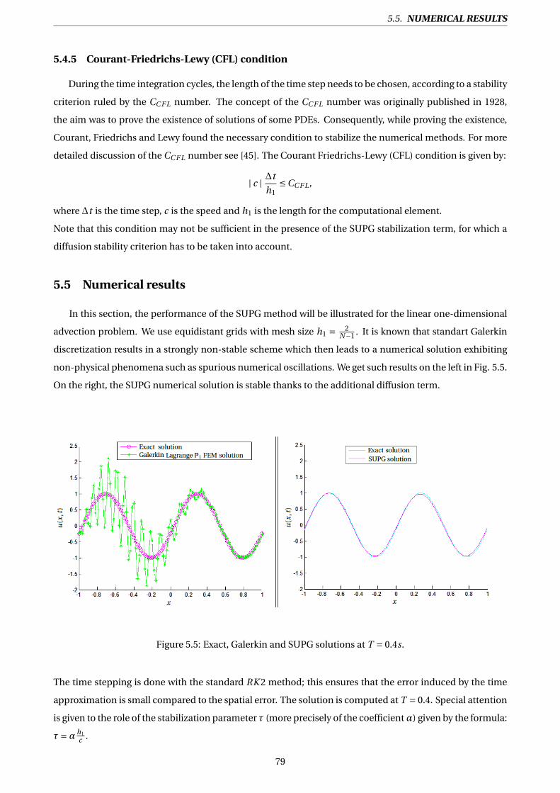
5.5. NUMERICAL RESULTS
5.4.5 Courant-Friedrichs-Lewy (CFL) condition
During the time integration cycles, the length of the time step needs to be chosen, according to a stability
criterion ruled by the CC F L number. The concept of the CC F L number was originally published in 1928,
the aim was to prove the existence of solutions of some PDEs. Consequently, while proving the existence,
Courant, Friedrichs and Lewy found the necessary condition to stabilize the numerical methods. For more
detailed discussion of the CC F L number see [45]. The Courant Friedrichs-Lewy (CFL) condition is given by:
| c | ∆t
h1≤CC F L ,
where ∆t is the time step, c is the speed and h1 is the length for the computational element.
Note that this condition may not be sufficient in the presence of the SUPG stabilization term, for which a
diffusion stability criterion has to be taken into account.
5.5 Numerical results
In this section, the performance of the SUPG method will be illustrated for the linear one-dimensional
advection problem. We use equidistant grids with mesh size h1 = 2N−1 . It is known that standart Galerkin
discretization results in a strongly non-stable scheme which then leads to a numerical solution exhibiting
non-physical phenomena such as spurious numerical oscillations. We get such results on the left in Fig. 5.5.
On the right, the SUPG numerical solution is stable thanks to the additional diffusion term.
Figure 5.5: Exact, Galerkin and SUPG solutions at T = 0.4s.
The time stepping is done with the standard RK 2 method; this ensures that the error induced by the time
approximation is small compared to the spatial error. The solution is computed at T = 0.4. Special attention
is given to the role of the stabilization parameter τ (more precisely of the coefficientα) given by the formula:
τ=αh1c .
79

CHAPTER 5. SUPG - FINITE ELEMENT METHOD
5.5.1 Influence of the SUPG parameter
The SUPG FEM contains a stabilization parameter τ for which a general "optimal" choice is not known.
It is pointed out that the optimal choice of this parameter is still an open question. The aim of this section is
to describe how the SUPG stabilization parameter impacts the solution for the one-dimensional advection
problem. The influence of this parameter on the numerical results is illustrated in Fig. 5.6.
Figure 5.6: SUPG FE P1 solution for different values of α ∈ [0,1].
80

5.5. NUMERICAL RESULTS
We can see clearly in Fig. 5.6 important oscillations for 0 ≤ α ≤ 0.01 and α ≥ 0.6. For α too small, the
stabilization effect is not strong enough to counterbalance the instability of Galerkin scheme. When α is
too large, oscillations are due to the violation of the stability criteria in RK time integration for diffusive
terms. For 0.01 <α≤ 0.5, we do not observe oscillations. However, a too large additional diffusion (α= 0.5)
impacts the accuracy of the solution, even if the scheme is stable. In what follows, we propose to determine
the optimal choice by studying the L2-error.
5.5.2 Error Estimates for the SUPG FE method
We want to evaluate the numerical behavior of the SUPG linear FEM for the problem (5.1), where an an-
alytic solution is explicitly known. The interest here is in the evaluation of the errors committed for different
mesh steps h1 as well as the order of convergence of the method. A mesh convergence study allows to test
the accuracy of the numerical method by numerically evaluating an order of accuracy. The error between
the approximate solution uh and the analytic solution uex for a final time T is determined in the standard
L2−norm:
∥ e(T ) ∥L2(Ω) = ∥ uex (x,T )−uh(x,T ) ∥L2(Ω)
=(∫Ω
(uex (x,T )−uh(x,T )
)2d x
) 12
=(
N−1∑k=1
∫ xk+1
xk
(sin(2π(x − cT ))−uh(x,T )
)2d x
) 12
.
Before we proceed further, let us denote by r the convergence rate of the SUPG FEM. We assume that a
norm ∥ e(T ) ∥L2(Ω) of the computational error behaves according to the formula:
∥ e(T ) ∥L2(Ω)=Cr hr1 ,
where Cr > 0 is a constant, h1 the mesh size and r ∈R.
Let ∥ e1(T ) ∥L2(Ω) and ∥ e2(T ) ∥L2(Ω) be computational errors of the numerical solutions obtained on two dif-
ferent meshes h1 and h2, respectively. Then we obtain:
r = ln( ∥ e2(T ) ∥L2(Ω)
)− ln( ∥ e1(T ) ∥L2(Ω)
)ln
(h2
)− ln(h1
) .
Table 5.1 shows the error of the SUPG-P1FEM numerical approximations in L2-norm for various number of
degrees of freedom (d.o.f.) (notice that the number of d.o.f. is equal to N ) and coefficient of the stabilization
parameter α ∈ [0,1]. The L2-errors of the numerical approximations are depicted in Fig. 5.7 for different
values of α in log scale.
81

CHAPTER 5. SUPG - FINITE ELEMENT METHOD
∥ e(T ) ∥L2
α d .o. f . = 16 d .o. f . = 32 d .o. f . = 64 d .o. f . = 128 d .o. f . = 256 d .o. f . = 512 d .o. f . = 1024
1 8.001E +003 1.706E +008 1.703E +017 3.509E +035 2.997E +072 4.359E +146 −0.9 7.027E +002 1.237E +006 7.943E +012 6.610E +026 9.141E +054 3.474E +111 −0.8 0.475E +002 5.341E +003 1.366E +008 1.694E +017 5.118E +035 9.248E +072 5.991E +1470.7 2.464 13.560 8.560E +002 6.146E +006 5.871E +014 1.035E +031 6.346E +0630.6 0.846 0.656 0.434 0.255 0.139 7.299E −002 3.737E −0020.5 0.807 0.598 0.381 0.218 0.117 6.131E −002 3.127E −0020.4 0.752 0.526 0.322 0.180 9.581E −002 4.943E −002 2.511E −0020.3 0.667 0.435 0.255 0.139 7.298E −002 3.737E −002 1.891E −0020.2 0.538 0.321 0.179 9.571E −002 4.941E −002 2.511E −002 1.266E −0020.1 0.362 0.177 9.491E −002 4.925E −002 2.508E −002 1.265E −002 6.355E −003
0.09 0.345 0.161 8.585E −002 4.444E −002 2.260E −002 1.139E −002 5.722E −0030.08 0.330 0.145 7.669E −002 3.961E −002 2.012E −002 1.013E −002 5.088E −0030.07 0.317 0.129 6.745E −002 3.475E −002 1.762E −002 8.876E −003 4.453E −0030.06 0.308 0.113 5.814E −002 2.986E −002 1.513E −002 7.613E −003 3.818E −0030.05 0.304 9.779E −002 4.880E −002 2.495E −002 1.262E −002 6.348E −003 3.183E −0030.04 0.305 8.323E −002 3.948E −002 2.001E −002 1.011E −002 5.082E −003 2.547E −0030.03 0.313 7.084E −002 3.034E −002 1.510E −002 7.597E −003 3.813E −003 1.911E −0030.02 0.329 6.257E −002 2.180E −002 1.024E −002 5.085E −003 2.569E −003 9.900E −0030.01 0.353 6.107E −002 1.53E −002 5.669E −003 2.662E −003 1.837E −002 84.784
Table 5.1: L2-errors of the SUPG FE P1 method for the one-dimensional advection problem.
Figure 5.7: Convergence in number of d.o.f. for different choices of α.
We observe that the convergence rates obtained are lower than the optimal rate expected (of value 2). As
shown in [58] [91], this reduction of the convergence rate is due to the use of the mass lumping procedure,
in addition to the use of the stabilization term (for some τ values).
82

5.6. SUPG FE METHOD FOR HIGH-ORDER ELEMENTS
α d .o. f . = 16 d .o. f . = 32 d .o. f . = 64 d .o. f . = 128 d .o. f . = 256 d .o. f . = 512 d .o. f . = 1024
0.6 − 0.36 0.59 0.76 0.87 0.93 0.970.5 − 0.3 0.65 0.8 0.91 0.93 0.970.4 − 0.51 0.7 0.84 0.91 0.95 0.980.3 − 0.61 0.77 0.87 0.93 0.97 0.980.2 − 0.74 0.84 0.91 0.94 0.97 10.1 − 1.03 0.92 0.94 0.97 1 1
0.09 − 1.12 0.91 0.95 0.77 1.2 10.08 − 1.2 0.92 0.95 0.98 1 1.020.07 − 1.3 0.94 0.96 0.98 1 10.06 − 1.5 0.96 0.96 0.98 1 10.05 − 1.6 1 0.98 0.98 1 10.04 − 1.7 1.07 0.98 0.99 0.98 10.03 − 2 1.22 1 1 0.99 1
Table 5.2: Convergence rates.
5.6 SUPG FE method for high-order elements
In some applications, the affine approximation on each element of the mesh Ωi = [xi , xi+1] can be con-
sidered as not good enough in the sense that it provides an approximate function that is too far from the
exact function u. To overcome this problem, we can approximate u on each mesh by polynomials of higher
degree. We now extend the above considerations to higher-order finite-elements. We particularly focus our
attention in this section on the FE approximation P2, which consists in approaching the solution u by a
continuous function onΩ and a polynomial of degree 2 on each elementΩi .
Now, let us revisit the one-dimensional advection problem that is given in (5.6) and we examine the quadratic
Lagrange bases functions. These are constructed by adding an extra node xi+ 12
at the midpoints of each
Ωi = [xi , xi+1],
xi+ 12= xi + h1
2, ∀1 ≤ i ≤ N −1.
Figure 5.8: Uniform P2 mesh of [a,b].
83

CHAPTER 5. SUPG - FINITE ELEMENT METHOD
The FEM for Lagrange P2 elements involves the discrete space:
V 2h =
wh ∈C 0([−1,1]) wh |Ωi
∈P2 ∀1 ≤ i ≤ N −1 such that wh(a) = u2a
.
These spaces are composed of piecewise polynomials functions (polynomials of degree less than or equal
to 2). The P2 FEM consists in applying the internal variational approximation approach to these spaces.
V 2h is a subspace of H 1(Ω) of dimension 2N − 1. As with the piecewice-linear basis, one basis function is
associated with each node. Those associated with vertices are:
φ j (x) =
2(x−x j−1)(x−x j− 1
2)
h21
if x j−1 ≤ x ≤ x j ,
2(x j+1−x)(x j+ 1
2−x)
h21
if x j ≤ x ≤ x j+1,
0 otherwise,
(5.23)
and those associated with element midpoint are:
φ j+ 12
(x) =
4
(x j+1−x)(x−x j )
h21
if x j ≤ x ≤ x j+1,
0 otherwise.
(5.24)
These functions are shown in Fig. 5.9. Their construction (to be described) involves satisfying: φ j (xi ) = δi j
φ j (xi+ 12
) = 0and
φ j+ 12
(xi ) = 0
φ j+ 12
(xi+1) = δi j
Figure 5.9: Global shape functions for the space V 2h .
84

5.6. SUPG FE METHOD FOR HIGH-ORDER ELEMENTS
The SUPG variational formulation of the problem (5.6) consists in finding uh ∈ H 1([0,T ],V 2h ). Every
function uh ∈V 2h defined by its values at the mesh vertices (xi )1≤i≤N and at the midpoints (xi+ 1
2)1≤i≤N−1:
uh(x, t ) =N∑
j=1u j (t )φ j (x)+
N−1∑j=1
u j+ 12
(t )φ j+ 12
(x) ∀x ∈Ω.
Furthermore, since it is enough to use basis functions of V 2h as test functions v , the discrete weak formula-
tion can be rewritten in form of linear differential system, wich can be described as follows:
M s2∂tU = R s
2U + c(U2a −U2b
). (5.25)
Since the shape functions φi have a compact support, the matrices M s2 and R s
2 are mostly composed of
zeros. In contrast to the Lagrange P1 FEM, the matrices M s2 and R s
2 are no longer tridiagonal matrices. Their
elements are given by:
(M s
2
)i j =
∫Ωφ j (x)φi (x)d x +
∫Ωφ j+ 1
2(x)φi+ 1
2(x)d x
+ τc(N−1∑
k=1
∫ xk+1
xk
φ′i (x)φ j (x)d x +
N−1∑k=1
∫ xk+1
xk
φ′i+ 1
2(x)φ j+ 1
2(x)d x
),
and
(R s
2
)i j = c
(∫Ωφ′
i (x)φ j (x)d x +∫Ωφ′
i+ 12
(x)φ j+ 12
(x)d x)
− τc2(N−1∑
k=1
∫ xk+1
xk
φ′j (x)φ′
i (x)d x +N−1∑k=1
∫ xk+1
xk
φ′j+ 1
2(x)φ′
i+ 12
(x)d x),
where,
U2a =
sin(2π(−1− ct ))
0...
0
∈R2N−1 and U2b =
0
0...
uN
∈R2N−1
85

CHAPTER 5. SUPG - FINITE ELEMENT METHOD
In this case, the elementary contributions of the elementΩi = [xi , xi+1] to the stiffness matrix and to the
mass matrix are given by the 3×3 elementary matrices R s2e |Ωi
and M s2e |Ωi
:
R s2e |Ωi
=
−7τc2
3h1
−2c3 + 8τc2
3h1
c6 − τc2
3h1
2c3 + 8τc2
3h1
−16τc2
3h1
−2c3 + 8τc2
3h1
−c6 − τc2
3h1
2c3 + 8τc2
3h1
−7τc2
3h1
,
and
M s2e |Ωi
=
2h115
h115 − 2τc
3−h130 + τc
6
h115 + 2τc
38h115
h115 − 2τc
3
−h130 − τc
6h115 + 2τc
32h115
.
In the present case of P2 elements, Simpson’s rule can be derived. In particular, let the basis function φ j
be tabulated at points x j , x j+1 ∀1 ≤ j ≤ N −1 (equally spaced by distance h1), and midpoint x j+ 12= x j+x j+1
2 .
Then Simpson’s rule states that:∫ x j+1
x j
f (x)d x ≈ x j+1 −x j
6
(f (x j )+4 f (x j+ 1
2)+ f (x j+1)
). (5.26)
Since it uses quadratic polynomials to approximate functions, Simpson’s rule actually gives exact results
when approximating integrals of polynomials up to cubic degree.
Hence, the so-called lumped mass matrix M s2 thus computed is diagonal and is given by:
M s2L |Ωi
= 1
6
h1 −3τc 0 0
0 4h1 0
0 0 h1 +3τc
.
Upon replacing the consistent mass matrix M s2 by the lumped mass matrix M s
2L , we rewrite the matrix form
5.25 as follows:
∂tU = (M s
2L
)−1R s2U + c
(M s
2L
)−1(U2a −U2b
). (5.27)
86
5.6. SUPG FE METHOD FOR HIGH-ORDER ELEMENTS
5.6.1 Matrix assembly
The construction of the global mass and stiffness matrices, M s2L and R s
2 is often referred to as "assem-
bling" due to its method of construction. The assembly is obtained algorithmically using a loop over all
mesh elements Ωi , ∀1 ≤ i ≤ N −1 (which is composed of three nodes x j , x j+ 12
and x j+1) and adding their
contributions to the corresponding coefficients of the global system. It is more convenient to loop over each
element instead of looping over all basis functions at the outer loop.
The algorithm of constructing the global mass and stiffness matrices M s2L and R s
2 can be described as fol-
lows:
Pseudo-code of matrix assembly:
1. For k = 1 : N −1
2. For i = 1 : 3
3. ig = 2(k −1)+ i
4. For j = 1 : 3
5. jg = 2(k −1)+ j
6. M s2L(ig , jg ) = M s
2L(ig , jg )+ms2e (i , j )
7. R s2(ig , jg ) = R s
2(ig , jg )+ r s2e (i , j )
8. End (loop j )
9. End (loop i )
10. End (loop k)
The space semidiscrete problem (5.25) represents a system of ODEs, which has to be solved with the RK
schemes. The choice of the timestep that ensures a stable scheme, for the quadratic Lagrange P2 SUPG FE
method is based on the condition:
∆t ≤ h1CC F L
2 | c | .
87

CHAPTER 5. SUPG - FINITE ELEMENT METHOD
5.6.2 Numerical results
To give an illustration of the SUPG quadratic Lagrange FEM in conjunction with RK 2 method for the
temporal discretization, some numerical results are presented in this section. The exact and numerical
solutions of the problem (5.6) investigated by these methods, are depicted in Fig. 5.10 for different choices
of the coefficient α. The numerical behavior of the method is evaluated on the spacial domain [−1,1],
which is subdivided into N −1 uniformly distributed subintervals with a number of d .o. f . = 2N −1 , and
time domain [0,T ] where T > 0 is considered as the final time.
Figure 5.10: SUPG quadratic Lagrange P2 FEM in conjunction with RK 2 for the 1D advection problem.
88

5.6. SUPG FE METHOD FOR HIGH-ORDER ELEMENTS
Figure 5.10 shows that the SUPG solution obtained for τ defined by α ≥ 0.2 contains large spurious
oscillations whereas they are less important for α≤ 0.01. These oscillations disappear if α ∈ [0.05,0.1]. The
results shown in Table 5.3 confirm what has been observed in Fig. 5.10. These results are similar as those
obtained with SUPG P1 method.
5.6.3 Accuracy study
To assess the quality of the numerical approximations, we compare the approximate solutions with the
exact solution in terms of L2-norm. The errors of the numerical approximations for various number of d.o.f.
and choice of the coefficient α are shown in Table 5.3 for the RK 2 time discretization and in Table 5.4 for
the RK 4 time discretization: surprisingly, no stabilization was required in this case.
e(T )α d .o. f . = 16 d .o. f . = 32 d .o. f . = 64 d .o. f . = 128 d .o. f . = 256 d .o. f . = 512 d .o. f . = 1024
α= 0.9 2.555E +064 1.042E +131 − − − − −α= 0.8 9.798E +059 1.274E +122 − − − − −α= 0.7 8.426E +054 7.731E +111 − − − − −α= 0.6 9.837E +048 8.491E +099 − − − − −α= 0.5 7.048E +041 3.430E +085 − − − − −α= 0.4 8.064E +032 3.402E +067 4.392E +137 − − − −α= 0.3 1.290E +021 5.983E +043 9.608E +089 − − − −α= 0.2 1.001E +005 8.691E +010 4.601E +023 1.004E +050 3.818E +103 − −α= 0.1 0.032 7.875E −003 1.921E −003 4.739E −004 1.176E −004 2.932E −005 7.318E −006α= 0.09 0.032 7.897E −003 1.924E −003 4.744E −004 1.177E −004 2.932E −005 7.320E −006α= 0.08 0.032 7.925E −003 1.929E −003 4.75E −004 1.178E −004 2.933E −005 7.373E −006α= 0.07 0.033 7.958E −003 1.935E −003 4.757E −004 1.179E −004 2.935E −005 1.528E −005α= 0.06 0.033 7.996E −003 1.942E −003 4.768E −004 1.180E −004 2.945E −005 6.492E −004α= 0.05 0.033 8.04E −003 1.952E −003 4.782E −004 1.182E −004 4.259E −005 1.574E −001α= 0.04 0.032 8.308E −003 1.965E −003 4.803E −004 1.190E −004 1.772E −003 6.227E +002α= 0.03 0.033 8.125E −003 1.982E −003 4.838E −004 2.473E −004 0.845 1.769E +008α= 0.02 0.033 8.141E −003 2.003E −003 5.043E −004 2.504E −002 1.494E +004 7.326E +016α= 0.01 0.033 8.111E −003 2.022E −003 5.050E −003 65.454 1.592E +011 1.301E +031
Table 5.3: The L2-error norm in function of the choice of the stabilization parameter α.
89

CHAPTER 5. SUPG - FINITE ELEMENT METHOD
These results have been obtain without stabilization.
e(T )d .o. f . = 16 d .o. f . = 32 d .o. f . = 64 d .o. f . = 128 d .o. f . = 256 d .o. f . = 512 d .o. f . = 1024
1.420E −02 3.406E −03 8.476E −04 2.1154E −04 5.285E −05 1.321E −05 3.302E −06
Table 5.4: The L2-error norm for RK 4 time discretization.
In Fig. 5.11 we show the L2-error norm depending on the numbers of d.o.f for the optimal choice of α.
5.7 Conclusion
In the present chapter we have focuced our attention to the SUPG FEM. As mentioned before, no stan-
dard scheme has been formulated to select the stabilisation parameter τ, which depends on the problem
and the grid size. In our work, we have assumed that the stabilisation parameter τ takes the form:
τ=αh
c,
and thus we have focused our attention on the selection of α ∈ [0,1].
In order to have a precise idea for the linear and quadratic Lagrange SUPG FEM in conjunction with RK 2
for time discretization, we represented the L2-error norm for an optimal choice for each method for a suc-
cessive refinement of the mesh. Even if the convergence rate does not seem to be strongly impacted by the
choice of α, the influence of the stabilization on the error level was reported.
Figure 5.11: L2-error for the advection problem with the linear and quadratic Lagrange FEM.
90


CONCLUSION
DAns ce chapitre, l’équation d’advection pure unidimensionnelle est étudiée. Le but
est de mettre en évidence l’instabilité de la méthode de Galerkin pour un tel prob-
lème et d’analyser la façon dont les méthodes stabilisées apportent une solution
pour construire un schéma à la fois robuste et précis. Pour cela, on a introduit une perturbation des fonc-
tions tests pondérées par un paramètre de stabilisation afin d’assurer la précision et la consistance du
schéma numérique. C’est dans ce contexte qu’on a introduit les méthodes de type Petrov-Galerkin: SUPG,
PSPG ou encore GLS. Comme cela a déjà été dit, une approche éléments finis stabilisés s’appuie sur une for-
mulation éléments finis standard à laquelle s’ajoute un terme de stabilisation. Cela revient à passer d’une
méthode de Galerkin à une méthode de Petrov-Galerkin grâce à la modification des fonctions tests de la
formulation faible.
Dans le présent chapitre, nous avons concentré notre attention sur la méthode d’EF stabilisé SUPG,
pour Lagrange linéaire et quadratique en conjonction avec RK 2 et RK 4 pour la discrétisation temporelle.
Une attention particulière a été accordée à l’identification du paramètre de stabilisation τ de cette méthode
qui pondère les termes de stabilisation, et son influence sur l’erreur de la solution.
92


CH
AP
TE
R
6ISOGEOMETRIC ANALYSIS: B-SPLINE AS A FEM BASIS
ISogeometric Analysis (IGA) is a generalization of classical FEA. It was first introduced by
T.J.R. Hughes, J.A. Cottrell and Y. Bazilevs [43] with the main aim of closing the gap be-
tween the geometrical description and the analysis of engineering problems. The isoge-
ometric paradigm consists of using basis functions commonly found in CAD geometries such as B-spline,
to represent both the geometry and the physical fields in the solution of problems governed by partial dif-
ferential equations (PDEs) [43] [67]. However, Hughes and co-authors considered only elliptic or parabolic
problems so far. The objective of this chapter is to consider IGA in the hyperbolic context. This chapter
reviews the various computational procedures for IGA, by revisiting the one-dimensional advection prob-
lem that is given in (5.6). While in this chapter we use B-splines (due to the simplicity of the domain), it
is not hard to generalize it to other splines such as NURBS. Detailed comparisons between IGA and FEA
approaches are carried out.
6.1 IGA: a B-spline based approach
IGA employs the same mathematical foundations as FEA to obtain the numerical solutions of differen-
tial equations, but the idea behind IGA method is to use the same functions that define the physical domain
Ω⊂R2, to approach the solution. Although the main difference between FEA and IGA lies compactly in the
set of basis functions used, this change influences all steps of traditional FEA: preprocessing, solving and
postprocessing.
The basis functions of IGA B-splines (more generally NURBS) are defined on a parameter space (or param-
eter domain) that we denote Ω. It is defined by control points, and not nodes like discretized domain in
FEA. The input of node coordinates is replaced by coordinates of control points. Before we proceed further,
let us notice that the B-spline parameter space Ω corresponds to "patches" instead of elements. A patch
can be seen as a "macro-element", whereas knot intervals can be seen as traditional elements. Thus, the
94

6.1. IGA: A B-SPLINE BASED APPROACH
B-spline mapping transforms a patch of multiple elements in the parameter space into the physical space.
Each element in the physical space is the image of a corresponding element (knot interval) in the parameter
space, but the mapping itself is global to the whole patch, rather than to the elements themselves. We refer
to Fig. 6.1 for a schematic overview of this approach.
Figure 6.1: An example of a B-spline patch in physical space Ω, parametric space Ω, and the referenceelement Ω used to perform numerical integration.
6.1.1 Isogeometric discretisation
The parameter domain Ω is defined by the knot vectors Ξ1 and Ξ2:
Ξ1 =ξ1 = ... = ξp+1,ξp+2, ...,ξn ,ξn+1 = ... = ξn+p+1
,
and
Ξ2 =η1 = ... = ηq+1,ηq+2, ...,ηm ,ηm+1 = ... = ηm+q+1
,
where, p and q are prescribed degrees, ξi and η j are the i -th and j -th knots, i , j are the knots indices,
i = 1,2, ...,n +p +1, j = 1,2, ...,m +q +1 and n,m equals the number of basis functions.
95

CHAPTER 6. ISOGEOMETRIC ANALYSIS: B-SPLINE AS A FEM BASIS
IGA allows to control the geometry and variables at the control points, in contrast to FEA which writes
these quantities at the nodes. The transformation of the parametric domain Ω to the physical domain Ω is
introduced:
T : Ω 7−→Ω
(ξ,η) 7−→ (x(ξ,η), y(ξ,η)
).
Note that this transformation is not linear and is simply defined by the parametric representation of the
computational domain. Unless otherwise specified, we assume that the mapping T to be invertible and its
inverse:
T−1 :Ω 7−→ Ω,
transforms points in the physical domain to their corresponding parameter values. Any point of coordinate
(x, y) in the physical domain Ω is mapped to a point (ξ,η) in the parametric domain Ω. The mapping from
the parametric domain to the physical domain is defined by associating a control net Pi j to each basis
function in such a way that: (x(ξ,η), y(ξ,η)
)= n∑i=1
m∑j=1
Ni ,p (ξ)N j ,q (η)Pi j .
Thus, the basis functions in the physical domainΩ are defined by:
Ni j ,pq (x, y) =Ni j ,pq(T(ξ,η)
)=Ni j ,pq (ξ,η) =Ni ,p (ξ)N j ,q (η).
It is important to point out that in some applications (which uses the simple geometries such as square,
circle/ellipse), the computational domain can be modeled straightforwardly with only a single patch. But
for more complex geometries, it is not possible to describe the physical computational domain with just
one geometrical mappingT, we need to use multi-patch geometries (we refer the reader to [26] [40]). In this
thesis we focus on single-patch geometries for the sake of simplicity but the extension is quite simple.
In an isoparametric formulation, the variable field is approximated by the same shape functions:
u(ξ,η) =n∑
i=1
m∑j=1
Ni ,p (ξ)N j ,q (η)ui j .
Hence, the variable u is obtained as functions of ξ and η. Here ui j denotes the value of the variable field
u corresponding to the control net Pi j . It is therefore referred to as a control variable or more generally a
degree of freedom (d.o.f.). Note that B-spline representations are not interpolatory, so ui j is not the solution
value at the location Pi j .
6.1.2 Computational procedures for IGA
The fact that the functions are defined in the parametric space while the space derivatives are with
respect to the coordinates of the physical space makes it necessary to compute the Jacobian matrix of the
geometric mapping defined as:
96

6.2. ISOGEOMETRIC FE FORMULATION
J = ∂x
∂ξ∂x∂η
∂y∂ξ
∂y∂η
.
We also highlight that for the one-dimensional case, the Jacobian matrix reduces to:
Jξ =∂x
∂ξ=
n∑i=1
(∂Ni ,p (ξ)
∂ξ
)Pi ,
and we denote, J−1ξ
= ∂ξ∂x .
We will try to give an idea of the calculation of the integrals. Integrals over the entire geometry (physical
domain) are split into elementary integrals over a domain denoted by Ωe . Let f be a function of the two
variables x and y . Then,∫Ω
f(x, y)dΩ =Nel∑e=1
∫Ωe
f(x, y)dΩe
=Nel∑e=1
∫Ωe
f(T(ξ,η))dΩe
=Nel∑e=1
∫Ωe
f(ξ,η) | J | dΩe
=Nel∑e=1
∫Ω
f(ξ, η
) | J || J | dΩ (via the mapping T(F i g . 6.1)).
We also highlight that ξ and η on the parent domain Ω are given as functions of ξ and η on parametric
domain Ωi j = [ξi ,ξi+1]× [η j ,η j+1]:
ξ= 1
2
((ξi+1 −ξi )ξ+ (ξi+1 +ξi )
),
η= 1
2
((η j+1 −η j )η+ (η j+1 +η j )
).
Therefore, the Jacobian of this transformation reads:
| J |= 1
4
(ξi+1 −ξi
)(η j+1 −η j
).
For the one-dimensional case | J | reduces to:
| J |= 1
2
(ξi+1 −ξi
).
6.2 Isogeometric FE formulation
After a general description of the physical domain, geometrical mappings, and an introduction of no-
tations for the IG method, we will discusses in this section specific details of the implementation of IGFE
method.
97

CHAPTER 6. ISOGEOMETRIC ANALYSIS: B-SPLINE AS A FEM BASIS
The IGM based on B-splines is not much different than the classical FEM. Subtle differences are intro-
duced due to the non-interpolatory character of B-splines and the definition of an element.
We focus now on the one-dimensional advection problem that is given in the previous chapter by:
∂u(x,t )∂t + c ∂u(x,t )
∂x = 0 ∀(x, t ) ∈ [a,b]× [0,T ],
u(x,0) = u0(x) ∀x ∈ [a,b],
u(a, t ) = ua(t ) ∀t ∈ [0,T ],
(6.1)
with,
u0(x) = sin(2πx) ∀x ∈ [a,b],
ua(t ) = sin(2π(−1− ct )
) ∀t ∈ [0,T ].
In order to solve Eq. (6.1), we consider a spatial discretization of its domain by means of B-spline functions
IGA in the framework of the Galerkin method and we need to write the weak form. Before we proceed
further, let us define:
VN := spanNi , for i = 1, ..,n
,
VN := spanNi , for i = 1, ..,n
.
According to the IGA concept, these spaces will be used to build the test function spaces for the approxima-
tion of (6.1). However, we define a subspace V B which only span a finite number of B-spline basis functions.
That is:
V B = V∩VN,
where,
V :=
wB ∈ H 1(Ω) such that wB (a) = ua
.
For IGA in the framework of the Galerkin method, we start by multiplying the strong form (6.1) by a B-spline
test function vB and integrate over the domainΩ, then using Green’s first identity and applying the bound-
ary conditions we finally get:
∫Ω∂t u(x, t )vB (x)d x − c
∫Ω
u(x, t )∂x vB (x)d x = cuavB (a)− cubvB (b).
As in the previous chapter, we introduce a SUPG stabilization term yielding:
Find u ∈ H 1([0,T ],V B ) such that :∫Ω
∂u(x, t )
∂tvB (x)d x − c
∫Ω
u(x, t )∂vB (x)
∂xd x +τc
n−p∑k=1
∫ xk+1
xk
∂u(x, t )
∂t
∂vB (x)
∂xd x
+τc2n−p∑k=1
∫ xk+1
xk
∂u(x, t )
∂x
∂vB (x)
∂xd x = cuavB (a)− cubvB (b) ∀vB ∈ H 1([a,b]).
98
6.2. ISOGEOMETRIC FE FORMULATION
The solution u is obtained by solving the finite-dimensional problem: Find u ∈ H 1([0,T ],V B ) such that :
asp (u, vB ) = Lsp (vB ) ∀vB ∈ H 1([a,b]).(6.2)
Where, asp : V B ×H 1([a,b]) 7−→R is given by:
asp (u, vB ) =∫Ω
∂u(x, t )
∂tvB (x)d x − c
∫Ω
u(x, t )∂vB (x)
∂xd x +τc
n−p∑k=1
∫ xk+1
xk
∂u(x, t )
∂t
∂vB (x)
∂xd x
+ τc2n−p∑k=1
∫ xk+1
xk
∂u(x, t )
∂x
∂vB (x)
∂xd x,
and
Lsp : H 1([a,b]) 7−→R, that contains the right hand side term of (6.2) and
Lsp (vB ) = cuavB (a)− cubvB (b).
Galerkin’s method consists in constructing finite-dimensional approximations of V B , denoted V Bh . Strictly
speaking, these will be subsets such that: V Bh ⊂ V B . Therefore, the SUPG formulation of this problem can
be written:Find uh ∈ H 1([0,T ],V B
h ) such that :∫Ω
∂uh(x, t )
∂tvB
h (x)d x − c∫Ω
uh(x, t )∂vB
h (x)
∂xd x +τc
n−p∑k=1
∫ xk+1
xk
∂uh(x, t )
∂t
∂vBh (x)
∂xd x
+τc2 ∑n−pk=1
∫ xk+1xk
∂uh (x,t )∂x
∂vBh (x)∂x d x − cua(t )vB
h (a)+ cub(t )vBh (b) = 0.
According to the isogeometric paradigm, the solution uh from the IGA space H 1([0,T ],V Bh ) can be repre-
sented using B-spline basis functions for the one-dimensional case, in the form:
uh(x, t ) =n∑
j=1N j ,p (x)u j (t ),
where n is the number of basis functions which is equal to the number of control points and the degrees
of freedom (d.o.f.) of uh associated with the control points, respectively. This representation is similar to
that used in classical FEM. By choosing the test function vBh equal to the B-spline basis function Ni ,p , the
Galerkin IGA scheme reads as follows:
Find u1,u2, ...,un such that :n∑
j=1
(∫ΩN j ,p (x)Ni ,p (x)
∂u j (t )
∂td x +τc
n−p∑k=1
∫ xk+1
xk
N j ,p (x)N′i ,p (x)u j (t )d x − c
∫ΩN j ,p (x)N′
i ,p (x)u j (t )
+τc2n−p∑k=1
∫ xk+1
xk
N′i ,p (x)N′
j ,p (x)u j (t )d x)= cuaNi ,p (a)− cubNi ,p (b) ∀i = 1, ...,n.
Finally, we obtain the linear system which is:
M B∂tU = RBU + cU Ba − cU B
b , (6.3)
similar to that resulting from the FEM in conjunction with SUPG.
99

CHAPTER 6. ISOGEOMETRIC ANALYSIS: B-SPLINE AS A FEM BASIS
The elementary mass and stiffness matrices are defined by:
M Bi j =
∫ΩN j ,p (x)Ni ,p (x)d x +τc
n−p∑k=1
∫ xk+1
xk
N j ,p (x)N′i ,p (x)d x ∀i , j = 1, ...,n,
and
RBi j = c
∫ΩN j ,p (x)N′
i ,p (x)d x −τc2n−p∑k=1
∫ xk+1
xk
N′j ,p (x)N′
i ,p (x)d x ∀i , j = 1, ...,n,
and the right-hand side given by:
U Ba =
sin(2π(−1− ct ))
0...
0
∈Rn , and U Bb =
0
0...
un
∈Rn .
We note that on the elementΩ j , only p+1 B-splines functionsN j ,p ,N j+1,p , ...,N j+p,p non zero and only p+1
derivativesN′j ,p ,N′
j+1,p , ...,N′j+p,p are non zero. The correspond matrices are therefore sparse.
By performing the integration in the parametric space and using the Jacobian of the B-spline mapping, we
get:
M Bi j =
∫Ω
N j ,p (ξ)Ni ,p (ξ)Jξdξ+τcn−p∑k=1
∫Ωk
N j ,p (ξ)N ′i ,p (ξ)dξ,
and
RBi j = c
∫Ω
N j ,p (ξ)N ′i ,p (ξ)dξ−τc2
n−p∑k=1
∫Ωk
N ′j ,p (ξ)N ′
i ,p (ξ)J−1ξ dξ.
By interpreting the integration in the parent element, we get:
M Bi j =
∫Ω
N j ,p (ξ)Ni ,p (ξ) Jξd ξ+τcn−p∑k=1
∫Ωk
N j ,p (ξ)N ′i ,p (ξ)d ξ,
and
RBi j = c
∫Ω
N j ,p (ξ)N ′i ,p (ξ)d ξ−τc2
n−p∑k=1
∫Ωk
N ′j ,p (ξ)N ′
i ,p (ξ) J−1ξ
d ξ.
Contrary to Lagrange elements, the element integrals appearing are evaluated using Gauss points via Gaus-
sian quadrature which can be described as follows:∫Ω
N j ,p (ξ)Ni ,p (ξ)d ξ'nG∑
k=1N j ,p (X G
k )Ni ,p (X Gk )ωG
k ,
where nG are the number of integration points X Gk , ωG
k is the weight corresponding to the k-th integration
point (see Appendix A). This approach is more flexible than the use of analytical integration.
The global mass and stiffness matrices are obtained using the assembly technique.
100

6.3. NUMERICAL RESULTS
As mentionned before, we focus in this thesis on the RK method for the time integration. The ODE (6.3)
is integrated in time by means of a second and fourth-order RK schemes. In one spatial dimension, a space
discretization using polynomials basis functions of degree p, associated to a (p+1)-stage RK time integrator
of order p +1, the stability limit for the CFL number is defined by:
∆t | c |h
≤CC F L .
where h is the size of the image of the knot interval considered.
6.3 Numerical results
The standard Galerkin formulation for the advection problem produces unstable discretizations. This
is well known in FEA for the Lagrange P1 and P2 elements, and unfortunately, is also observed for the lin-
ear and quadratic B-splines-based approach as we can see in this section. We investigate the ability of the
isogeometric approach based on B-splines of arbitrary degree, in conjunction with SUPG, to solve advec-
tion problem. In all calculations the mesh is uniform with element size length h = 2n−p . The solutions are
calculated from p = 1 to p = 4. Notice that in the case of linear and quadratic B-spline, the standard SUPG
formulation is used with the choice of the stabilization parameter τ = αhc while for the cubic and quartic
B-spline it is important to point out that the method has been found stable, and therefore τ= 0.
Figure 6.2: (a) SUPG B-spline linear solution for the advection problem (α= 0.1). (b) SUPG FEM P1 for theadvection problem (α= 0.1) at T = 0.4s.
Due to the equivalence of hat shape functions and linear B-spline functions, the linear FEM and IGA give
the same results (as shown in Fig. 7.3). However, this is not the case for representations of higher degree.
If one compares quadratic B-spline basis functions with basis functions based on Lagrange interpolating
polynomials, one can notice some critical differences.
101

CHAPTER 6. ISOGEOMETRIC ANALYSIS: B-SPLINE AS A FEM BASIS
6.3.1 Influence of the SUPG stabilization parameter τ for the quadratic B-spline
We first consider the case of quadratic B-spline. The results for the advection problem for different
choices of α ∈ [0,1] are presented in the Fig. 6.3. The plotting routine sampled the solution with a grid of
uniformly distributed points.
Figure 6.3: SUPG quadratic B-spline solutions in conjunction with RK 2 for the advection problem.
These results are very similar to those obtained with Lagrange quadratic elements in Fig. 5.10.
102

6.3. NUMERICAL RESULTS
6.3.2 Error estimates for the quadratic B-spline
We define the error of the numerical solution as e(T ) = uex (x,T )−uh(x,T ). The L2(Ω)-norm of the error
is depicted in the Table 6.1 which is defined by:
∥ e(T ) ∥L2([−1,1])=∥ uex (x,T )−uh(x,T ) ∥L2([−1,1]) .
∥ e ∥L2
α n = 16 n = 32 n = 64 n = 128 n = 256 n = 512 n = 1024
0.9 6.7674E +057 3.972E +123 − − − − −0.8 6.773E +052 1.683E +113 − − − − −0.7 1.783E +047 4.567E +101 − − − − −0.6 8.831E +040 3.967E +088 − − − − −0.5 5.093E +033 4.032E +073 − − − − −0.4 1.721E +025 1.018E +056 4.240E +110 − − − −0.3 1.321E +015 5.248E +034 3.301E +073 − − − −0.2 1.400E +003 0.001E +008 7.434E +008 8.070E +019 1.180E +093 − −0.1 0.036 5.293E −003 2.552E −003 4.285E −005 1.671E −005 7.584E −006 2.860E −06
0.09 0.032 4.417E −003 2.185E −004 4.050E −005 1.669E −005 7.583E −006 2.860E −060.08 0.029 3.816E −03 1.938E −004 3.932E −005 1.668E −005 7.583E −006 2.860E −000.07 0.027 3.385E −003 1.765E −004 3.871E −005 1.668E −005 7.583E −006 2.860E −060.06 0.026 3.067E −003 1.639E −004 3.839E −005 1.667E −005 7.583E −006 2.860E −060.05 0.026 2.829E −003 1.547E −004 3.824E −005 1.667E −005 7.583E −006 2.860E −060.04 0.025 2.656E −003 1.478E −004 3.817E −005 1.667E −005 7.583E −006 2.860E −060.03 0.026 2.541E −003 1.428E −004 3.815E −005 1.667E −005 7.583E −006 2.859E −060.02 0.027 2.492E −003 1.401E −004 3.816E −005 1.667E −005 7.594E −006 1.322E −040.01 0.029 2.535E −003 1.418E −004 3.818E −005 1.670E −005 1.5091E −005 0.357
Table 6.1: The L2-error as function of the choice of the number of control points n and the stabilizationparameter α, for quadratic B-splines in conjunction with RK 2.
These results have been obtain without stabilization.
∥ e ∥L2
n = 16 n = 32 n = 64 n = 128 n = 256 n = 512 n = 1024
2.433E −02 1.246E −03 6.970E −05 6.195E −06 1.043E −06 1.235E −07 1.324E −08
Table 6.2: The L2-error as function of the choice of the number of control points n for quadratic B-splinesin conjunction with RK 4.
Convergence results in the L2-norm are shown in Tab. 6.1 and Tab. 6.2 for the quadratic B-spline. These re-
sults are also visualized in Fig. 6.4. As a result, the continuity of the basis is C 1 everywhere, for the quadratic
B-spline case. As can be seen, the L2-convergence for quadratic B-spline in conjunction with the RK 4 for
the temporal discretization is approximately 3. This is the best one could reasonably hope for.
103

CHAPTER 6. ISOGEOMETRIC ANALYSIS: B-SPLINE AS A FEM BASIS
6.4 Higher order B-spline
Table 6.3 shows the L2-error of the numerical approximations for various number of control point n and
order of B-spline. Those results are depicted in Figure 6.4. These results have been obtain without stabiliza-
tion.
Table 6.4 shows the convergence rates observed for different degrees. As can be seen, a sub-optimal rate of
the value 2 is obtained for quadratic basis in conjunction with RK 2, certainly due to the stabilization. For
quadratic basis in conjunction with RK 4, the optimal rate of the value 3 is obtained. For the degree p = 4,
the rate is limited by the use of RK 4 time integrator. For p = 3 a sub-optimal rate of value 3.5 is also ob-
served.
n = 16 n = 32 n = 64 n = 128 n = 256 n = 512 n = 1024p = 3 + RK 4 2.620E −03 4.502E −05 8.860E −07 3.024E −08 1.889E −09 1.900E −10 1.917E −11p = 4 + RK 4 2.528E −04 3.380E −06 1.223E −07 5.631E −09 3.211E −10 2.059E −11 1.483E −12
Table 6.3: Error measured in the L2-norm.
Figure 6.4: Convergence rates in the L2-norm.
p n = 16 n = 32 n = 64 n = 128 n = 256 n = 512 n = 1024
2( f or RK 2) − 2.77 2.11 2.1 2.01 2.01 22( f or RK 4) − 4.28 4.16 3.49 2.57 3.07 3.17
3 − 5.88 5.68 4.88 4.5 3.5 3.54 − 6.22 4.8 4.5 4.14 3.99 4
Table 6.4: Convergence rates.
104
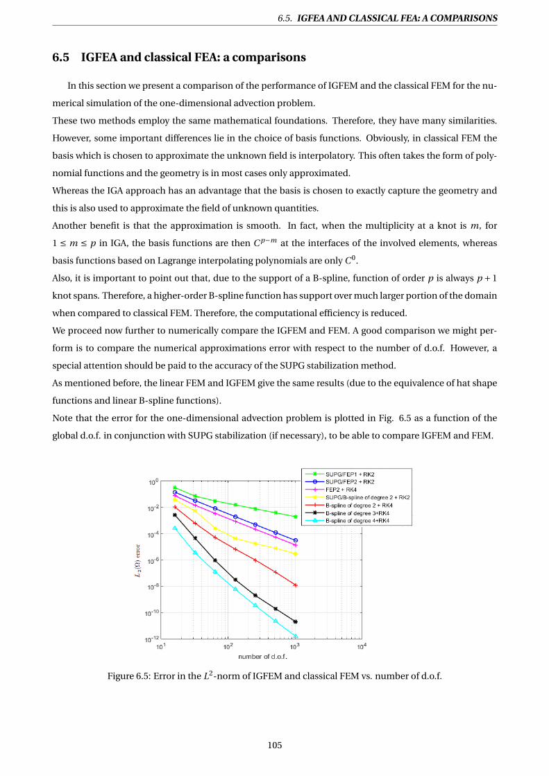
6.5. IGFEA AND CLASSICAL FEA: A COMPARISONS
6.5 IGFEA and classical FEA: a comparisons
In this section we present a comparison of the performance of IGFEM and the classical FEM for the nu-
merical simulation of the one-dimensional advection problem.
These two methods employ the same mathematical foundations. Therefore, they have many similarities.
However, some important differences lie in the choice of basis functions. Obviously, in classical FEM the
basis which is chosen to approximate the unknown field is interpolatory. This often takes the form of poly-
nomial functions and the geometry is in most cases only approximated.
Whereas the IGA approach has an advantage that the basis is chosen to exactly capture the geometry and
this is also used to approximate the field of unknown quantities.
Another benefit is that the approximation is smooth. In fact, when the multiplicity at a knot is m, for
1 ≤ m ≤ p in IGA, the basis functions are then C p−m at the interfaces of the involved elements, whereas
basis functions based on Lagrange interpolating polynomials are only C 0.
Also, it is important to point out that, due to the support of a B-spline, function of order p is always p +1
knot spans. Therefore, a higher-order B-spline function has support over much larger portion of the domain
when compared to classical FEM. Therefore, the computational efficiency is reduced.
We proceed now further to numerically compare the IGFEM and FEM. A good comparison we might per-
form is to compare the numerical approximations error with respect to the number of d.o.f. However, a
special attention should be paid to the accuracy of the SUPG stabilization method.
As mentioned before, the linear FEM and IGFEM give the same results (due to the equivalence of hat shape
functions and linear B-spline functions).
Note that the error for the one-dimensional advection problem is plotted in Fig. 6.5 as a function of the
global d.o.f. in conjunction with SUPG stabilization (if necessary), to be able to compare IGFEM and FEM.
Figure 6.5: Error in the L2-norm of IGFEM and classical FEM vs. number of d.o.f.
105

CHAPTER 6. ISOGEOMETRIC ANALYSIS: B-SPLINE AS A FEM BASIS
As one can see, results of this simple numerical test allow to make some conclusions. At first sight, the
graphs of Fig. 6.5 indicate that the slope of the error lines are not exactly 1, 2, 3 and 4 for 1st , 2nd , 3r d and
4th order elements, respectively. Moreover, we highlight that the values of the errors from the IGFEM are
far lower than those of the FEM.
We also note that, increasing the order of Lagrangian polynomials may increase the amplitude of oscillations
in the FEM. This problem is eliminated in IGA as a result of non-negativity and non-interpolatory nature
of the B-splines shape functions. In conclusion, we believe that the isogeometric approach has consider-
able potential in practical problem solving and is a promising alternative to current analysis procedures.
However, a possible drawback of the SUPG method is the sensitivity of the solution to the stabilization pa-
rameter, whose optimal value is not determined precisely by the available theory.
In the context of IGA, another approach we could go for is the application of DG method. Indeed, the major
argument for using DG methods lies in their ability to provide stable numerical methods for first order PDE
problems, for which classical FEM is well known to perform poorly. Therefore, we will introduce in the next
chapter a new DG method in the IG context, called IGDGM.
106


CONCLUSION
L’analyse isogéométrique (AIG) trouve ses origines depuis 2005 dans les travaux de
Hughes, Cottrell, et Bazilevs [43] avant d’être détaillée et formalisée dans le livre de
Cottrell et al. [24] dans un contexte de développement de nouveaux outils pour le
calcul numérique en ingénierie basée sur la simulation, celle-ci introduit un nouveau paradigme pour ten-
ter de combler le fossé entre la MEF et la CAO.
L’idée principale de l’AIG est de modéliser exactement la géométrie avec des fonctions qui vont servir à ap-
proximer la solution, ces fonctions permettant une description paramétrique d’un domaine. Elles sont
définies dans un espace appelé espace paramétrique; la géométrie est définie dans un espace nommé
espace physique. La paramétrisation de la géométrie est obtenue par un morphisme non linéaire en-
tre l’espace paramétrique et l’espace physique défini à l’aide des fonctions B-splines. S’il est nécessaire
d’effectuer des intégrations lors du processus de résolution, elles sont effectuées élément par élément sur
un élément de référence obtenu par une transformation linéaire à partir de l’espace paramétrique.
On a introduit brièvement dans ce chapitre le contexte de l’AIG. Pour cela, on a commencé par rap-
peler les fondements et les premiers objectifs de la méthode. On se restreint aux B-splines mais on ne doute
pas de l’applicabilité des méthodes développées ici à d’autres représentation de l’AIG (comme NURBS), ces
fonctions possèdent en fait une continuité de classe supérieure, ce qui permet d’obtenir plus de précision
pour un même nombre de degrés de libertés comparé aux EF classiques.
Les travaux présentés dans ce chapitre ont pour objectif de mettre au point une méthode d’EF stabilisée, la
méthode SUPG pour un problème d’advection dans le cadre de l’AIG. L’idée principale est donc d’utiliser
les fonctions de base B-spline représentant la géométrie pour générer l’espace de recherche de la solution
au problème hyperbolique souhaité.
.
108

Part III
ISOGEOMETRIC DISCONTINUOUS
GALERKIN METHOD (IGDGM)
110

CH
AP
TE
R
7DISCONTINUOUS GALERKIN METHOD (DGM): FROM
CLASSICAL TO ISOGEOMETRIC
WE propose a method that combines isogeometric analysis (IGA) with the discontin-
uous Galerkin (DG) method for solving hyperbolic problems, namely the isogeo-
metric discontinuous Galerkin (IGDG) method that merges exact geometry with
high-order solution accuracy [54] [61]. In this chapter we formulate and analyze this method for the one-
dimensional advection problem. The solution of the problem is approximated in every sub-domain without
any continuity requirement for the discrete solution at the interfaces. Finally, we numerically compare the
performance of the IGDG method with the DGFE method.
7.1 Introduction and background
The discontinuous Galerkin finite element (DGFE) method was originally introduced in 1973 by Reed
and Hill [74], for the numerical solution of the nuclear transport PDE problem. Subsequently, the method
has found broad applications in large-scale data intensive science and engineering problems. DG is a class
of FEM that uses completely discontinuous basis functions. Thanks to their flexibility in local approxima-
tion, they offer good stability properties when approximating convection dominated problems [79] [93].
In contrast to the stabilized continuous Galerkin FEM, DG method produces stable discretizations for hy-
perbolic problems without the need for stabilization parameters, stabilization resulting from the use of up-
wind fluxes. Therefore, this method combines the best properties of the finite volume (FV) method and
continuous Galerkin FEM.
111

CHAPTER 7. DISCONTINUOUS GALERKIN METHOD (DGM): FROM CLASSICAL TO ISOGEOMETRIC
In fact, the FV method, which is well suited to hyperbolic conservation laws, can only use low-degree
polynomials to locally represent the solution. In contrast, FEM are unstable for hyperbolic problems and,
as seen in previous chapters, stabilization relies on tedious choice of a parameter. Therefore, the idea of this
method is to decompose the original problem into a set of subproblems, solved by using a FEM approach,
that are connected using an appropriate transmission condition (known as the numerical flux).
Although DG methods have gained increasing attention in large-scale modeling applications, a shortcom-
ing of the conventional DG methodology is the inability to fully recover complex underlying geometries in
the meshing domain. To overcome this problem, we combine IGA method with the DG method. As men-
tioned before, IGA is a computational technique that improves and generalizes the classical FE method.
The main benefit of this method is the exact representation of the geometry in the language of computer
aided design (CAD) tools. This simplifies the meshing as the computational mesh is directly created by the
engineer using the CAD tools.
The proposed IGDG method is the DG method formulated on elements that exactly preserve the geometry
generated by CAD tools while the PDE solution exhibits discontinuities at element interfaces. An important
property of B-spline in the context of DG is the ability to perform Bézier extraction. Bézier extraction pro-
vides the capability of recovering a local Bernstein-Bézier representation of the geometry from the global
B-spline CAD. In this chapter, we will discuss specific details of the implementation of IGDG method for the
one-dimensional linear advection problem in contrast to the DGFE method.
7.2 DGFE framework for one-dimensional scalar conservation law
The DGFE method was first designed as an effective numerical method for solving hyperbolic conser-
vation laws [72] [93]. In this section, we will present the details of the DGFE method, the stability analysis,
and the error estimates for the one-dimensional scalar conservation law given by:
∂u(x,t )∂t + ∂ f (u(x,t ))
∂x = 0 ∀(x, t ) ∈Ω× [0,T ],
u(x,0) = u0(x) ∀x ∈Ω,
u(a, t ) = ua(t ) ∀t ∈ [0,T ].
(7.1)
(withΩ= [a,b] and f ′(u) > 0 ∀x ∈Ω).
7.2.1 Discontinuous Galerkin-space discretization
In the DG method, the domainΩ= [a,b] is subdivided into a union of finite number Nel of cells Dk Nel
k=1,
each element being delimited by two nodes of coordinates x lk and xr
k , such that:
Ω= [a,b] =Nel⋃k=1
Dk with Dk⋂
Dl =; ∀1 ≤ k 6= l ≤ Nel
112

7.2. DGFE FRAMEWORK FOR ONE-DIMENSIONAL SCALAR CONSERVATION LAW
We note that: x l1 = a and xr
Nel= b.
We define uniform Nel cells Dk of length h by:
Dk = [x lk , xr
k ] and h= xrk −x l
k , ∀1 ≤ k ≤ Nel .
We denote by T the subdivision ofΩ into Nel elements Dk ,
T =Dk , 1 ≤ k ≤ Nel
.
The starting point for the derivation of a DG scheme is obtained by multiplying Eq. (7.1) by a polynomial
test function v on each cell and then integrating over an arbitrary subset Dk of T :∫Dk
∂u(x, t )
∂tv(x)d x +
∫Dk
∂ f (u(x, t ))
∂xv(x)d x = 0, ∀t ∈ [0,T ].
We underline that this integration is carried-out over a single element Dk and not over the whole computa-
tional domainΩ, as done in a classical FE approach. After integration by parts, one obtains:∫Dk
∂u(x, t )
∂tv(x)d x =
∫Dk
f (u(x, t ))∂v(x)
∂xd x + f
(u(x l
k , t ))− f
(u(xr
k , t )), ∀t ∈ [0,T ].
The DG method represents the unknowns like the FEM by piecewise polynomial functions, but unlike FEM
the polynomials are discontinuous at the cell interfaces. A numerical flux is defined at the cell interface
in the same way as for Finite Volume (FV) methods. So, on each cell Dk , the discrete unknown ukh is repre-
sented as a linear combination of well chosen basis functions of the space of polynomials of degree p. Then,
the finite-dimensional subspace Vp
h is defined as:
Vp
h =
v ∈ L2(Ω) | v|Dk∈Pp (Dk ) ∀1 ≤ k ≤ Nel , Dk ∈T
,
wherePp (Dk ) represents the space of polynomials of degree up to p defined on the element Dk . Notice that
functions in Vp
h are discontinuous across cell interfaces.
As a consequence, the flux f evaluated at the interfaces of the element Dk is replaced by a numerical flux
function f , due to the fact that uh is a priori discontinuous at the interfaces. Therefore, the local approxi-
mate solution ukh is then determined as the unique solution of the following weak formulation:
For each element Dk ∈T :∫Dk
∂ukh(x, t )
∂tvh(x)d x =
∫Dk
f(uk
h(x, t ))∂vh(x)
∂xd x + f l
k − f rk , ∀t ∈ [0,T ], ∀vh ∈ V
ph . (7.2)
113

CHAPTER 7. DISCONTINUOUS GALERKIN METHOD (DGM): FROM CLASSICAL TO ISOGEOMETRIC
Note that, for the boundary element D1, the numerical flux for the left edge is defined using the given
boundary condition:
f l1 = f (ua(t )).
For the element DNel , the numerical flux for the right edge is evaluated using interior solution:
f rNel
= f (uNel
h (t )).
For interior interfaces, a basic idea is to use a numerical flux f that is defined according to the left and right
values of the solution at the interface, as in a classical FV approach:
f lk = f
(uk−1
h (x l−k , t ),uk
h(x l+k , t )
),
f rk = f
(uk
h(xr−k , t ),uk+1
h (xr+k , t )
),
with, ukh = uh |Dk
.
Naturally, the choice of the flux is important.
7.2.2 Numerical flux
To complete the definition of the approximate solution uh , it only remains to choose the numerical flux
f . An approximation to the true flux [5] at an element’s interface is defined by considering the following
conditions:
• A numerical flux is defined using interface solution values regardless of the polynomial space chosen
for the solution,
f = f(uk+
h ,uk−h
),
where uk+h and uk−
h are the fields on the two sides of the element interface Γk .
• Consistency: For continuous solutions, the numerical flux must be equivalent to the normal flux at
the interface:
f (ukh ,uk
h) = f (ukh).
• Conservation: If a piecewise constant approximation is used, the discretization results in a monotone
FV scheme. This is ensured if we have a conservative flux,
f(uk+
h ,uk−h
)− f(uk−
h ,uk+h
)= 0.
114

7.2. DGFE FRAMEWORK FOR ONE-DIMENSIONAL SCALAR CONSERVATION LAW
There are many possible choices of the numerical flux [71] satisfying the above properties:
Central flux:
fC E N = 1
2
(f (uk−
h )+ f (uk+h )
).
Upwind flux:
fUp =
f (uk−
h ) if f ′(ukh) ≥ 0,
f (uk+h ) else.
Lax-Friedrichs flux:
fLF = 1
2
(f (uk−
h )+ f (uk+h )
)+ CLF
2
(uk−
h −uk+h
)= fC E N + CLF
2
(uk−
h −uk+h
),
where CLF is the maximum wave speed at the interface:
CLF = max | f ′(uh) | for min(uk−h ,uk+
h ) ≤ uh ≤ max(uk−h ,uk+
h ).
The Lax-Friedrichs flux adds an extra diffusive term to the central flux in an attempt to smear out insta-
bilities. We will focus on the Lax-Friedrichs flux, in the following work, which is a classical choice in DG
methods.
7.2.3 Elementary linear system
Returning now to Eq. (7.2) and substituting the local solution approximation in element Dk , there are
(p +1) equations to be solved for each component of the field corresponding to the (p +1) degrees of free-
dom. Indeed, if a local basis ofPp (Dk ) is chosen and denoted as(ϕk
j (x))
j=1,...,p+1, for x ∈Dk , we can express
the local numerical solution ukh as:
ukh(x, t ) = uh |Dk
(x, t ) =p+1∑j=1
ukj (t )ϕk
j (x), ∀x ∈Dk , ∀t ∈ [0,T ].
If Lagrange polynomials are used as local basis, ukj corresponds to the solution value in element k at inter-
polation point j .
Since the support of the basis functions is restricted to the element Dk , the left-hand side of equation 7.2 is
simply the product of a local mass matrixMk of size (p +1)× (p +1) with the vector of the time-derivative of
the degrees of freedom ∂t uk for the elementDk . The right-hand side represents the residual for the element
Dk , composed of a volume integral Rk and fluxes at the interfaces Fl and Fr , which ensures the coupling
with solution in neighboring elements.
115

CHAPTER 7. DISCONTINUOUS GALERKIN METHOD (DGM): FROM CLASSICAL TO ISOGEOMETRIC
Therefore, we should solve the following local system for each element k:
Mk∂t uk = Rk (uk )+ f lk − f r
k ∀t ∈ [0,T ] k = 1, ..., Nel , (7.3)
for the coefficients:
uk =
uk1
uk2...
ukp+1
.
The global solution u(x, t ) is then assumed to be approximated by the piecewise p-th order polynomial
approximation uh(x, t ):
u(x, t ) ' uh(x, t ) =Nel⊕k=1
ukh(x, t ),
defined as the direct sum of the Nel local polynomial solutions ukh(x, t ).
7.3 Computation of residual and mass matrix
Contrary to the FEM, only local matrices on each element (in practice only the elementary matrices
on the reference interval [−1,1]) need to be assembled. The coefficients of the local mass matrix for the
element Dk are:
(Mk )i j =∫Dk
ϕki (x)ϕk
j (x)d x i , j = 1, ..., p +1.
The first contribution to the residual is the integral over each element Dk of the flux multiplied by the test
function gradient: (Rk (uk )
)i j =
∫Dk
f(uk
h(x, t ))
j∂xϕ
ki (x)d x i , j = 1, ..., p +1.
The numerical integration is performed using the Gauss-Legendre quadrature rules described above.
7.4 CFL condition for DG Method
An important feature of the above-presented method is the use of a local mass matrix, which results
from the local support of basis functions. As a consequence, the local mass matrix can be inverted easily
before time integration and the method is well suited to high-order explicit time integration, like RK meth-
ods, and is highly parallelizable. Therefore, in the present work, RK 2 and RK 4 are used for time integration.
Because we are focusing on DG schemes, we discuss the limitation on the CC F L number when the DG
method is used in conjunction with the RK time integration approach. A stability condition on the size
of the timestep must indeed be satisfied. It corresponds to the Courant Friedrichs-Lewy (CFL) condition:
λ∆t
h≤CC F L ,
where λ= maxu | f ′(u) |, h is the smallest element width, and ∆t is the length of the time step.
116
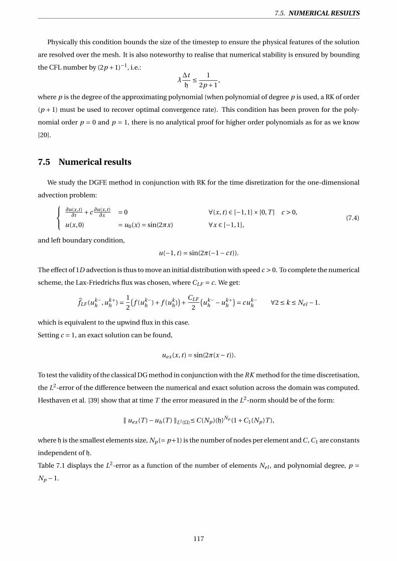
7.5. NUMERICAL RESULTS
Physically this condition bounds the size of the timestep to ensure the physical features of the solution
are resolved over the mesh. It is also noteworthy to realise that numerical stability is ensured by bounding
the CFL number by (2p +1)−1, i.e.:
λ∆t
h≤ 1
2p +1,
where p is the degree of the approximating polynomial (when polynomial of degree p is used, a RK of order
(p + 1) must be used to recover optimal convergence rate). This condition has been proven for the poly-
nomial order p = 0 and p = 1, there is no analytical proof for higher order polynomials as for as we know
[20].
7.5 Numerical results
We study the DGFE method in conjunction with RK for the time disretization for the one-dimensional
advection problem:∂u(x,t )∂t + c ∂u(x,t )
∂x = 0 ∀(x, t ) ∈ [−1,1]× [0,T ] c > 0,
u(x,0) = u0(x) = sin(2πx) ∀x ∈ [−1,1],(7.4)
and left boundary condition,
u(−1, t ) = sin(2π(−1− ct )).
The effect of 1D advection is thus to move an initial distribution with speed c > 0. To complete the numerical
scheme, the Lax-Friedrichs flux was chosen, where CLF = c. We get:
fLF (uk−h ,uk+
h ) = 1
2
(f (uk−
h )+ f (ukh)
)+ CLF
2
(uk−
h −uk+h
)= cuk−h ∀2 ≤ k ≤ Nel −1.
which is equivalent to the upwind flux in this case.
Setting c = 1, an exact solution can be found,
uex (x, t ) = sin(2π(x − t )).
To test the validity of the classical DG method in conjunction with the RK method for the time discretisation,
the L2-error of the difference between the numerical and exact solution across the domain was computed.
Hesthaven et al. [39] show that at time T the error measured in the L2-norm should be of the form:
∥ uex (T )−uh(T ) ∥L2(Ω)≤C (Np )(h)Np (1+C1(Np )T ),
where h is the smallest elements size, Np (= p+1) is the number of nodes per element and C , C1 are constants
independent of h.
Table 7.1 displays the L2-error as a function of the number of elements Nel , and polynomial degree, p =Np −1.
117

CHAPTER 7. DISCONTINUOUS GALERKIN METHOD (DGM): FROM CLASSICAL TO ISOGEOMETRIC
Nel 16 32 64 128 256 512 1024
p = 1 6.0454E −02 1.528E −02 3.797E −03 9.449E −04 2.450E −04 5.963E −05 1.495E −05r ate − 1.98 2 2 1.94 2.03 1.99
p = 2 5.521E −03 6.896E −04 8.635E −05 1.077E −05 1.360E −06 1.593E −07 1.950E −08r ate − 3 2.99 3 2.98 3.09 3.03
Table 7.1: L2-errors for the 1D advection problem.
As we can see, Table 7.1 demonstrates that greater accuracy can be achieved by either increasing the
polynomial order or increasing the number of elements in the domain. The convergence rates were esti-
mated by fixing the polynomial degree, and measuring the L2-error as a function of the number of elements.
Assuming a relationship of the form:
∥ uex (T )−uh(T ) ∥L2(Ω)=C (T )(h)r ate , (7.5)
the convergence rate is estimated as the best slope fit of ln( ∥ uex (T )−uh(T ) ∥L2(Ω)
)against ln
(Nel
)for each
polynomials degree, as demonstrated in Fig. 7.1. The graphs indicate that r ate ≈ p +1, in agreement with
the estimate (7.5), which corresponds to the optimal rate.
Figure 7.1: L2-errors for the 1D advection problem using the DGFE method in conjunction with the RKmethod for a sinusoidal initial condition and Lax-Friedrichs flux.
118
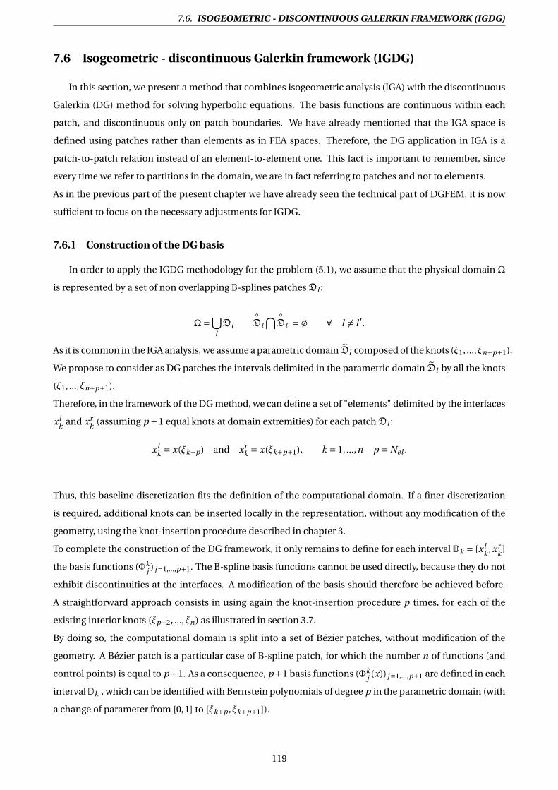
7.6. ISOGEOMETRIC - DISCONTINUOUS GALERKIN FRAMEWORK (IGDG)
7.6 Isogeometric - discontinuous Galerkin framework (IGDG)
In this section, we present a method that combines isogeometric analysis (IGA) with the discontinuous
Galerkin (DG) method for solving hyperbolic equations. The basis functions are continuous within each
patch, and discontinuous only on patch boundaries. We have already mentioned that the IGA space is
defined using patches rather than elements as in FEA spaces. Therefore, the DG application in IGA is a
patch-to-patch relation instead of an element-to-element one. This fact is important to remember, since
every time we refer to partitions in the domain, we are in fact referring to patches and not to elements.
As in the previous part of the present chapter we have already seen the technical part of DGFEM, it is now
sufficient to focus on the necessary adjustments for IGDG.
7.6.1 Construction of the DG basis
In order to apply the IGDG methodology for the problem (5.1), we assume that the physical domain Ω
is represented by a set of non overlapping B-splines patches Dl :
Ω=⋃lDl
Dl
⋂ Dl ′ =; ∀ l 6= l ′.
As it is common in the IGA analysis, we assume a parametric domain Dl composed of the knots (ξ1, ...,ξn+p+1).
We propose to consider as DG patches the intervals delimited in the parametric domain Dl by all the knots
(ξ1, ...,ξn+p+1).
Therefore, in the framework of the DG method, we can define a set of "elements" delimited by the interfaces
x lk and xr
k (assuming p +1 equal knots at domain extremities) for each patch Dl :
x lk = x(ξk+p ) and xr
k = x(ξk+p+1), k = 1, ...,n −p = Nel .
Thus, this baseline discretization fits the definition of the computational domain. If a finer discretization
is required, additional knots can be inserted locally in the representation, without any modification of the
geometry, using the knot-insertion procedure described in chapter 3.
To complete the construction of the DG framework, it only remains to define for each interval Dk = [x lk , xr
k ]
the basis functions (Φkj ) j=1,...,p+1. The B-spline basis functions cannot be used directly, because they do not
exhibit discontinuities at the interfaces. A modification of the basis should therefore be achieved before.
A straightforward approach consists in using again the knot-insertion procedure p times, for each of the
existing interior knots (ξp+2, ...,ξn) as illustrated in section 3.7.
By doing so, the computational domain is split into a set of Bézier patches, without modification of the
geometry. A Bézier patch is a particular case of B-spline patch, for which the number n of functions (and
control points) is equal to p+1. As a consequence, p+1 basis functions (Φkj (x)) j=1,...,p+1 are defined in each
intervalDk , which can be identified with Bernstein polynomials of degree p in the parametric domain (with
a change of parameter from [0,1] to [ξk+p ,ξk+p+1]).
119

CHAPTER 7. DISCONTINUOUS GALERKIN METHOD (DGM): FROM CLASSICAL TO ISOGEOMETRIC
In practice, basis functions used to represent the solution in the physical domain are defined in the
parametric domain by:
Φ j (x)|Dk=Φk
j (x(ξ))
Bk,pj (x) = B k,p
j (ξ) if x ∈Dk ,
0 otherwise,(7.6)
where B k,pj is the j -th Bernstein polynomial of degree p defined over the interval ]ξk+p ,ξk+p+1[.
The generation of the Discontinuous Galerkin basis from a B-spline (or NURBS) representation is illustrated
in Fig. 7.2:
Figure 7.2: Bézier decomposition (bottom) from a quadratic B-spline basis (top) by knot insertion.
120

7.6. ISOGEOMETRIC - DISCONTINUOUS GALERKIN FRAMEWORK (IGDG)
The resulting representation has several suitable properties:
• (Φkj ) j=1,...,p+1 are non-zero for x ∈]x(ξk+p ), x(ξk+p+1)[.
• (Φkj ) j=1,...,p+1 are C∞ for x ∈]x(ξk+p ), x(ξk+p+1)[.
•Φk1 andΦk
p+1 are equal to one at x+(ξk+p ) and x−(ξk+p+1).
•p+1∑j=1Φk
j (x) = 1 ∀x ∈]x(ξk+p ), x(ξk+p )[ (partition of unity).
• uh |Dk(x+(ξk+p )) = uk
1 (local solution interpolates first degree of freedom).
• uh |Dk(x−(ξk+p+1)) = uk
p+1 (local solution interpolates last degree of freedom).
• minj
ukj ≤ uh |Dk
≤ maxj
ukj (convex hull property).
These properties will be exploited to define an efficient numerical procedure, as described below.
7.6.2 Isogeometric discontinuous Galerkin approximation spaces
Let us now consider the physical element Dk , that can be exactly parametrized with a mapping T:
T : Dk 7−→Dk , ξ 7−→ x(ξ).
Thus, any point of coordinate x in the physical domain Dk is mapped to a point of parameter ξ in the
parametric domain Dk . The transformation is defined by associating a control point to each basis function:
x(ξ) =p+1∑j=1
B kj ,p (ξ)P j .
P j , for j = 1, ..., p +1 are defined by the knot insertion procedure as described above.
We will revisit the one-dimensional advection problem that is given in (5.1). Using the Bernstein basis func-
tions in the element Dk , uh |Dkis described as:
uh |Dk(x, t ) = uk
h(x, t ) =p+1∑j=1
Bkj ,p (x)uk
j (t ).
For the derivation of a IGDG scheme, equation (5.1) is multiplied by a polynomial test function on each local
patch Dk , ∀1 ≤ k ≤ Nel which can be choosen equal to the Bernstein basis function and after integration by
parts and introducing the numerical flux f , we get:
p+1∑j=1
∂t ukj (t )
∫Dk
Bki ,p (x)Bk
j ,p (x)d x = cp+1∑j=1
ukj (t )
∫Dk
Bkj ,p (x)∂xB
ki ,p (x)d x+ f (x l
k , t )− f (xrk , t )∀t ∈ [0,T ] k = 1, ..., Nel .
121

CHAPTER 7. DISCONTINUOUS GALERKIN METHOD (DGM): FROM CLASSICAL TO ISOGEOMETRIC
Since the support of the basis functions is restricted to the elementDk , the left-hand side of the previous
equation is simply the product of a local mass matrix M k of size (p +1)× (p +1) with the vector of the time-
derivative of the degrees of freedom ∂t uk for the elementDk . The right-hand side represents the residual for
the elementDk , composed of a volume integral Rk and fluxes at the interfaces f lk and f r
k , which ensures the
coupling with solution in neighboring elements. Therefore, the problem can be expressed in local matrix
form:
M k∂t uk =Rk uk + f lk − f r
k ∀t ∈ [0,T ] k = 1, ..., Nel . (7.7)
As for the DGFEM, for the first and last elements, the boundary fluxes f (ua) and f (ub) replace f l1 and f r
Nel
respectively. Note that, if one uses a piecewise constant representation p = 0, the mass matrix is just a scalar
equal to the element volume, the volumic residual is zero and one recovers a classical first-order FV method.
7.6.3 Computation of residual and mass matrix
The coefficients of the local mass matrix and stiffness matrix for the element Dk are:
(M k )i j =∫Dk
Bki ,p (x)Bk
j ,p (x)d x i , j = 1, ..., p +1,
(Rk )i j = c∫Dk
Bkj ,p (x)∂xB
ki ,p (x)d x i , j = 1, ..., p +1.
By performing the integration in the parametric cell Dk , we obtain:
(M k )i j =∫Dk
B ki ,p (ξ)B k
j ,p (ξ)(
J kξ
)dξ i , j = 1, ..., p +1,
and
(Rk )i j = c∫Dk
B kj ,p (ξ)∂ξB k
i ,p (ξ)dξ i , j = 1, ..., p +1,
where we denote J kξ= (
∂x∂ξ
)|Dk
.
The computation is achieved using Gauss-Legendre quadrature rules:
(M k )i j =nG∑l=1
B ki ,p
(X G (l )
)B k
j ,p
(X G (l )
)ωG
l
(J k
ˆX G (l )
)i , j = 1, ..., p +1,
where (X G (l ))l=1,...,nG and (ωGl )l=1,...,nG are quadrature abscissae and weights. Its inverse is computed nu-
merically, in a pre-processing phase.
(Rk )i j = cnG∑l=1
B kj ,p
(X G (l )
)∂ξB k
i ,p
(X G (l )
)ωG
l i , j = 1, ..., p +1.
The solution in each elementDk interpolates the local first and last degrees of freedom uk1 and uk
p+1. There-
fore, the flux computation only depends on the two degrees of freedom located at each interface:
f (x lk , t ) = f
(uk−1
p+1,uk1
),
f (xrk , t ) = f
(uk
p+1,uk+11
).
122
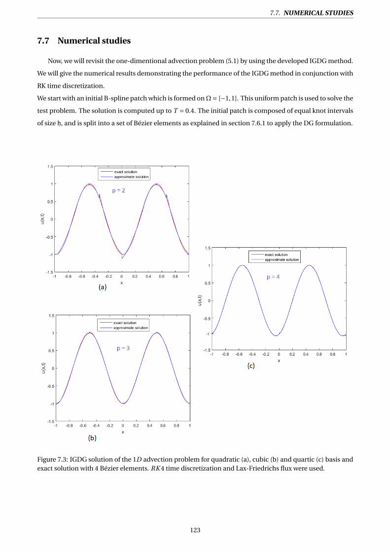
7.7. NUMERICAL STUDIES
7.7 Numerical studies
Now, we will revisit the one-dimentional advection problem (5.1) by using the developed IGDG method.
We will give the numerical results demonstrating the performance of the IGDG method in conjunction with
RK time discretization.
We start with an initial B-spline patch which is formed onΩ= [−1,1]. This uniform patch is used to solve the
test problem. The solution is computed up to T = 0.4. The initial patch is composed of equal knot intervals
of size h, and is split into a set of Bézier elements as explained in section 7.6.1 to apply the DG formulation.
Figure 7.3: IGDG solution of the 1D advection problem for quadratic (a), cubic (b) and quartic (c) basis andexact solution with 4 Bézier elements. RK 4 time discretization and Lax-Friedrichs flux were used.
123

CHAPTER 7. DISCONTINUOUS GALERKIN METHOD (DGM): FROM CLASSICAL TO ISOGEOMETRIC
The solutions obtained numerically are compared with the exact solutions in terms of L2 norm, for basic
functions of degrees 0, 1, 2, 3 and 4. The plots of the numerical solutions obtained using only 4 elements
and a quadratic, cubic and quartic basis are depicted in Figure 7.3.
We underline the accuracy of the solution obtained with a so small number of elements. Note also that the
discontinuities at the interfaces are decreasing as p increases.
One method to test the convergence of a spatial discretisation is by computing the error between the nu-
merical solution and the analytical one. The numerical approximation error in L2-norm:
∥ e ∥L2(Ω)=∥ uex (T )−uh(T ) ∥L2(Ω),
for various element sizes h and degrees p of the Bernstein basis and it is depicted in Fig.7.3. The conver-
gence rates are shown in Table 7.2 and Table 7.3. An optimal convergence rate is observed, the method
being of order p +1 with respect to L2− norm.
We notice that, as expected, the convergence rate is limited when using RK 2 time integrator. Therefore, we
employ RK 4 method to recover optimal convergence rate for p ≥ 2.
p h h2
h4
h8
h16 rate
0 4.649E −01 3.054E −01 1.699E −01 8.841E −02 4.477E −02 11 5.137E −02 1.322E −02 3.255E −03 8.176E −04 2.024E −04 22 4.255E −03 7.179E −04 1.594E −04 3.581E −05 8.652E −06 2.5
Table 7.2: L2−error for the IGDG method in conjunction with RK 2 time discretisation for various elementsizes and degree of Bézier basis p = 0,1,2.
p h h2
h4
h8
h16 rate
2 3.692E −03 4.671E −04 5.758E −05 7.083E −06 8.709E −07 33 9.299E −05 5.724E −06 3.322E −07 1.849E −08 1.062E −09 44 8.069E −06 2.497E −07 7.767E −09 2.359E −10 7.241E −12 5
Table 7.3: L2−error for the IGDG method in conjunction with RK 4 time discretisation for various elementsizes and degree of Bézier basis p = 2,3,4.
124
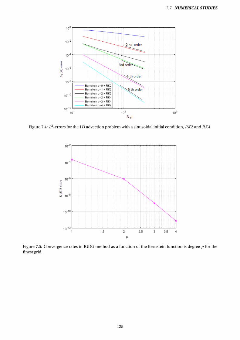
7.7. NUMERICAL STUDIES
Figure 7.4: L2-errors for the 1D advection problem with a sinusoidal initial condition, RK 2 and RK 4.
Figure 7.5: Convergence rates in IGDG method as a function of the Bernstein function is degree p for thefinest grid.
125

CHAPTER 7. DISCONTINUOUS GALERKIN METHOD (DGM): FROM CLASSICAL TO ISOGEOMETRIC
7.8 Conclusion and comparison
In this chapter a new family of discontinuous Galerkin methods which combines the IGA with the
DG method, called IGDG method, has been developed for the one-dimensional advection problem. Our
method takes advantage of both IGA and DG methods. In fact, DG methodology is adopted at Bézier patch
level, i.e., we employ the traditional IGA within each Bézier patch, and employ the DG method across the
patch interfaces to glue the multiple patches. Bézier patches, considered as elements, are constructed by
transformation of the initial B-spline domain. Due to IGA, all conic sections can be represented exactly,
thus eliminating the geometrical errors by the construction. Obviously, this property will be more evident
for 2D problems.
As mentioned before, the major reason for using DG methods lies with their ability to provide stable numer-
ical methods for first order PDE problems, for which classical FEM is well known to perform poorly. Due to
the piecewise discontinuity of basis functions, the DG method can be applied locally in each element. This
simplifies the implementation of the method, since the mass matrix becomes block diagonal and the solu-
tion of a large system is avoided. The solution for the whole computational domain is achieved by summing
over all the elements of the mesh.
Compared to SUPG-FEM for solving hyperbolic problems, an attractive feature of the DG method is that it
still uses the basic Galerkin method for the volume integrals, although this is extended by element boundary
integrals to achieve the ‘upwinding’. Because of the simple concept of the method it is basically the same
for any space dimension. The treatment of boundary conditions is also relatively easy.
126
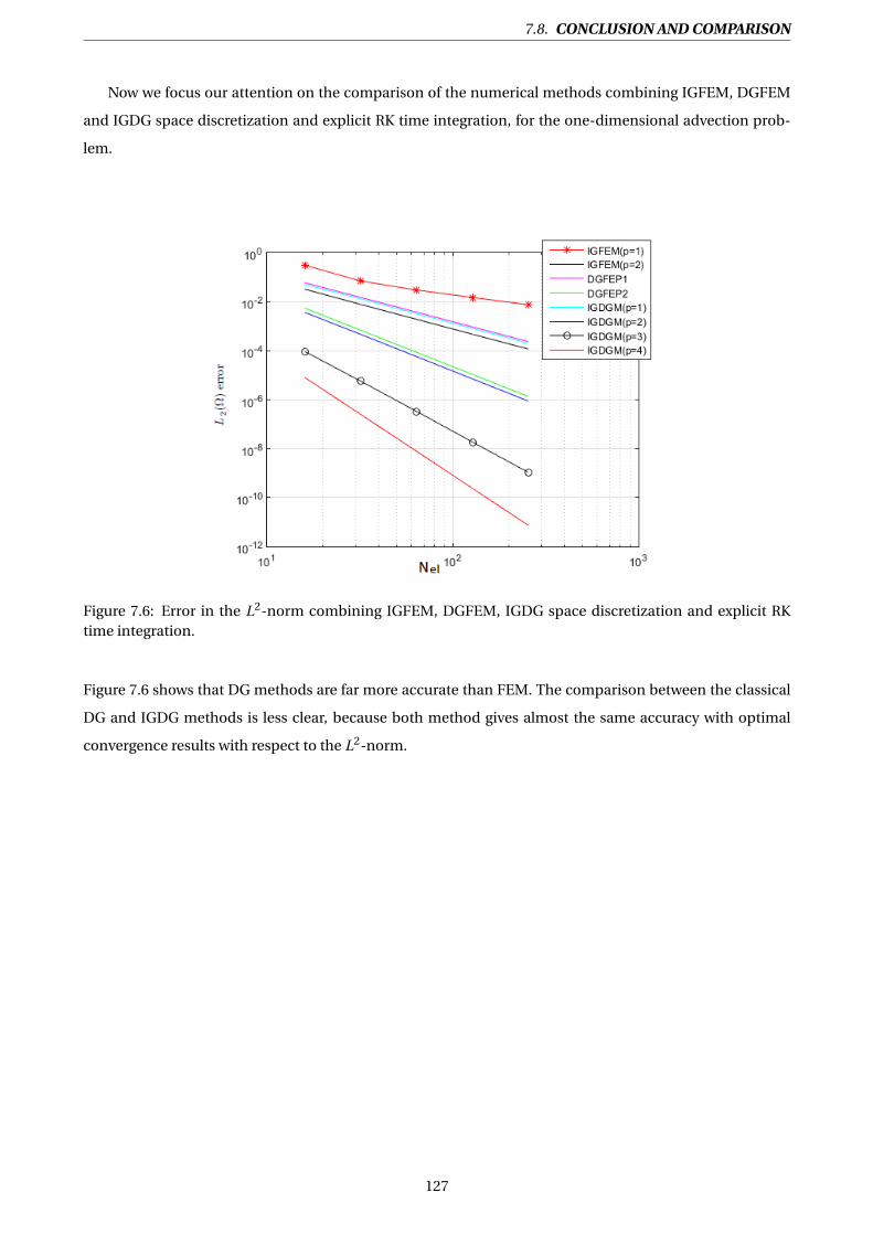
7.8. CONCLUSION AND COMPARISON
Now we focus our attention on the comparison of the numerical methods combining IGFEM, DGFEM
and IGDG space discretization and explicit RK time integration, for the one-dimensional advection prob-
lem.
Figure 7.6: Error in the L2-norm combining IGFEM, DGFEM, IGDG space discretization and explicit RKtime integration.
Figure 7.6 shows that DG methods are far more accurate than FEM. The comparison between the classical
DG and IGDG methods is less clear, because both method gives almost the same accuracy with optimal
convergence results with respect to the L2-norm.
127

CONCLUSION
LA méthode de Galerkin discontinue a initialement été introduite par Reed et Hill [74]
en 1973, pour la discrétisation des équations caractérisant le transport de neutrons.
C’est une méthode de Galerkin dont les fonctions tests sont polynomiales par morce-
aux, mais sans contrainte de continuité. La base de fonctions tests est définie localement sur des sous-
domaines par des polynômes d’ordre au plus p, et est identiquement nulle partout ailleurs. En conséquence,
la différence majeure avec les EF classiques provient de la non imposition de la continuité de la solution
numérique au niveau des frontières inter-éléments. L’intégration par parties conduit donc à l’apparition
d’intégrales sur ces frontières, qui sont évaluées de manière analogue à l’approche des volumes finis, en
introduisant des flux numériques des valeurs des fonctions de part et d’autre de l’interface.
Grâce à une grande flexibilité d’approximation locale, la méthode de GD offre de bonnes propriétés de
stabilité [79] [93]. Contrairement à la méthode de Galerkin continue stabilisée, la méthode de GD produit
des discrétisations stables pour les problèmes hyperboliques sans la nécessité de paramètres de stabilisa-
tion, la stabilisation résultant de l’utilisation de flux décentrés. Par conséquent, cette méthode combine les
meilleures propriétés de la méthode des volumes finis (VF) et de la méthode d’EF standard.
Bien que la méthode de GD ait attiré de plus en plus d’attention dans les applications de modélisation
à grande échelle, l’incapacité à récupérer exactement les géométries sous-jacentes complexes dans le do-
maine du maillage constitue une lacune de la méthodologie conventionnelle. Pour surmonter ce problème,
nous combinons l’AIG avec la méthode de GD. Comme indiqué précédemment, l’AIG est une technique
de calcul qui améliore et généralise la méthode d’EF classique. Le principal avantage de cette méthode est
la représentation exacte de la géométrie dans le langage des outils de conception assistée par ordinateur
(CAO).
La méthode de GD dans le cadre IG (IGGD) proposée est en fait une méthode de GD formulée sur
des éléments qui préservent exactement la géométrie générée par les outils de CAO, tandis que la solution
de l’EDP présente des discontinuités aux interfaces d’éléments. Une propriété importante des B-splines
dans le contexte de GD est la capacité à effectuer une extraction de Bézier. L’extraction de Bézier permet
de récupérer une représentation locale de Bernstein-Bézier de la géométrie à partir d’une B-spline glob-
ale. Dans ce chapitre, on a discuté des détails spécifiques de l’implémentation de la méthode IGGD pour le
problème unidimensinnel d’advection linéaire, ainsi que la méthode de GD classique.
129


Part IV
2D PROBLEM STUDY
131

CH
AP
TE
R
8IGDG: 2D ADVECTION PROBLEM
IN the previous chapter, we have described the various computational procedures for
IGDG analysis especially for the one-dimensional case. This chapter is devoted to the
extension to the two-dimensional case. The geometrical representation will obviously
play a more critical role in 2D cases and we will especially underline the tretment of the geometry. Numeri-
cal experiments validate the presented methodology.
8.1 Computational procedures in two dimensions
8.1.1 Preliminaries - IGDG notation
In order to apply the IGA methodology, the physical domainΩ is subdivided into B-spline patches De ,
S (Ω) := DeNpa
e=1 ,
such that:
Ω=⋃De with
D
e ⋂ D
l
=; ∀ e 6= l .
Moreover, we denote the interpatch boundary between the two patchesDe andDl by Γe,l and the collection
of all interfaces by Γ, i.e.,
Γe,l =De⋂
Dl and Γe := ⋃l>eΓe,l .
Furthermore, the boundary of the domainΩ is denoted by ∂Ω.
8.1.2 Isogeometric analysis (IGA): physical domain and geometrical mappings
The main idea behind the isogeometric approach is to discretize the unknowns of the problem with the
same set of basis functions that CAD employs for the construction of the geometries.
132

8.1. COMPUTATIONAL PROCEDURES IN TWO DIMENSIONS
We use the definitions from IGA that we introduced in chapter 6. In our specific case the physical domain
Ω⊂R2 is represented by a set of B-spline patches. Each B-spline patch denoted by De , is an image under a
B-spline mapping of a parametric domain De .
De =
X e = (xe , ye ) ∈R2 | X e =T(ξ,η) such that (ξ,η) ∈ De
,
where the transformation T is defined for all (ξ,η) ∈ De by:
T : De 7−→ De
(ξ,η) 7−→ (xe (ξ,η), ye (ξ,η)
).
Note that this transformation is non linear and is simply defined by the parametric representation of the
computational domain. Unless otherwise specified, we assume this mapping to be invertible. Its inverse:
T−1 :De 7−→ De ,
takes points in the physical domain to their corresponding parameter values. Figure 8.1 gives a schematic
overview of our proposed approach.
Figure 8.1: An example of a B-spline patch in physical space, parametric space, and the parent element usedto perform numerical integration.
133

CHAPTER 8. IGDG: 2D ADVECTION PROBLEM
8.1.3 Basic function space for the parametric domain and physical domain
In this section we focus on the construction of the basis functions. A C p−1 continuous basis Φ(ξ,η) is
constructed over the parameteric domain De . The basis is used to construct a geometric map T so that it
maps a point (ξ,η) ∈R2 in the parametric domain De to a point in De .
We have already stated that we consider elements to be the images of knot spans under the Bézier mapping.
We will denote these knot spans in the parameter space by De , and their image in the physical space as De ,
where e = 1, ...,Nel , with Nel being the total number of elements.
To implement the DG method in the isogeometric framework, i.e. based on a computational domain de-
fined from a B-spline representation, we must first define a set of elements, which are the supports of a
polynomial representation with discontinuities at each interface between elements. Given a B-spline sur-
face defining the computational domain, the insertions of knots p times are used for each of the existing
interior knot for each parametric direction sequentially. In doing so, the computational domain is divided
into a set of Bézier patches, without modification of the geometry. We remind that a Bézier patch is a special
case of B-spline patch, for which the number n of functions (and control points) is equal to p +1 (with p is
the degree of basis function).
Finally, all the Bézier patches created by the insertion process are considered as elements. Each element De
is therefore defined by (p +1)× (q +1) basis functions,(Bp,q (x, y)
)e , which can be identified with Bernstein
polynomials of degrees p and q :
(Bp,q (X )
)e =(Bp,q (x, y)
)e =(Bp,q(
T(ξ,η)))e =
(B p,q (ξ,η)
)e =
(B p (ξ)
)e ⊗(B q (η)
)e ∀(x, y) ∈De ,
0 otherwise.
where,(B p
i
)ei=1,...,p+1 and
(B q
j
)ej=1,...,q+1 are respectively the i−th and the j−th Bernstein polynomials of de-
gree p and q , defined on the interval [0,1] by:
(B p
i (ξ))e =C i
pξi (1−ξ)p−i ∀t ∈ [0,1] i = 0, ..., p.
A given control point P e will have local indices associated to the Bézier patch De . Thus, the geometrical
mapping local to element e can be defined as:
X e (ξ,η) = (xe (ξ,η), ye (ξ,η)
)= p+1∑i=1
q+1∑j=1
(B p
i (ξ))e(B q
j (η))e P e
i j .
Before we proceed further, we denote by J e the elementary Jacobian matrix of this transformation defined
in De by:
J e = ∂x
∂ξ∂x∂η
∂y∂ξ
∂y∂η
.
134

8.1. COMPUTATIONAL PROCEDURES IN TWO DIMENSIONS
Thus, we can also calculate the inverse of the elementary Jacobian matrix (J e )−1 given by:
(J e )−1 = 1
| J e |
∂y∂η −∂x
∂η
−∂y∂ξ
∂x∂ξ
= 1∂x∂ξ
∂y∂η − ∂x
∂η∂y∂ξ
∂y∂η −∂x
∂η
−∂y∂ξ
∂x∂ξ
= ∂ξ
∂x∂ξ∂y
∂η∂x
∂η∂y
.
Then, we define the test functions in the physical domainDe by using the same representation as the geom-
etry:
Φp,q (x, y)|De =(Φp,q (x, y)
)e =(Bp,q (x, y)
)e =(Bp,q(
T(ξ,η)))e
= (B p,q (ξ,η)
)e
=(B p (ξ)
)e ⊗(B q (η)
)e
=(Φp (ξ)
)e ⊗(Φq (η)
)e.
We also highlight that, ∀1 ≤ i ≤ p +1 and ∀1 ≤ j ≤ q +1,(Φp,q (x, y)
)e
i , j=
(B p (ξ)
)e
i
(B q (η)
)e
j
=(Φp (ξ)
)e
i
(Φq (η)
)e
j.
In addition, we need also to compute ∇Φe , which is the gradient in the Cartesian form:
∇Φe =
(∂Φp,q (x,y)
∂x
)e
(∂Φp,q (x,y)
∂y
)e
=
∂Φe
∂ξ∂ξ∂x + ∂Φe
∂η∂η∂x
∂Φe
∂ξ∂ξ∂y + ∂Φe
∂η∂η∂y
=
∂ξ∂x
∂η∂x
∂ξ∂y
∂η∂y
∂Φe
∂ξ
∂Φe
∂η
∇Φe = ∂Φe
∂ξ
∂Φe
∂η
= ∂x
∂ξ∂y∂ξ
∂x∂η
∂y∂η
∂Φe
∂x
∂Φe
∂y
= (J e)T ∇Φe .
Finally, one obtains:
∇Φe = (J e)T ∇Φe ,
∇Φe = ((J e )T )−1∇Φe .
8.1.4 Numerical integration
In this thesis we use Gaussian quadrature as a choice of numerical integration. To do this, we will need
to map our functions over to a reference square (ξ, η) ∈ D= [−1,1]× [−1,1]. While this is common for most
FEM as well, we have the additional mapping from the parametric space to the physical space. The first one
is an affine mapping (see Fig. 8.1):
T : D 7−→ De .
135

CHAPTER 8. IGDG: 2D ADVECTION PROBLEM
The numerical integration has to take place in the reference square, while all basis functions are defined
over the parametric domain and the differential equation is formulated in the physical space. Therefore, a
typical integration writes:
∫De
(Φ
p,qi , j (x, y)
)edDe =
∫De
(B
p,qi , j (T(ξ,η))
)edDe
=∫De
(Bi ,p (ξ,η)
)e(B j ,q (ξ,η)
)e | J e (ξ,η)| dDe
=∫D
(Bi ,p (ξ)
)e(B j ,q (η)
)e | J e (ξ, η)| | J e (ξ,η)| dD,
8.2 2D advection problem: IGDG space semi-discretization
In the following, we describe the discretization of the transient, bi-dimensional, linear conservation law
or transport equation over a domainΩ⊂R2 with periodic boundary conditions by the IGDG method: ∂t u +∇· (−→c u(x, y, t )) = 0 ∀(x, y, t ) ∈Ω× [0,T ],
u(x, y,0) = u0(x, y) ∀(x, y) ∈Ω,(8.1)
where u(x, y, t ) is a scalar quantity transported by a continuous velocity field −→c = (cx ,cy )t .
Similarly as in the previous chapter, we derive the IGDG space semidiscretization leading to a system of
ordinary differential equations. As a matter of fact, the IGDG method for multi-dimensional conservation
law has the same structure it has for one-dimensional scalar conservation laws, we only need to describe
the DG-space discretization.
Applying a IGDG method, the solution u is approximated by uh ∈Vp , which we assume to have the following
form:
ueh(x, y, t ) =
p+1∑i=1
q+1∑j=1
(Bi ,p (ξ)
)e(B j ,q (η)
)eue
i j (t ),
where uei j : [0,T ] 7−→R, ∀ 1 ≤ i ≤ p +1, 1 ≤ j ≤ q +1 are local unknown coefficients.
Before we proceed further, let us put veh ∈Vp
h , the approximate solution that will be sought for each t ∈ [0,T ]
in the finite-dimensional space:
Vph =
v := v(x(ξ,η), y(ξ,η)) ∈ L2(Ω), v|De ∈ span
B e,
where B e is the set of (p +1)× (q +1) Bernstein polynomials defined over De .
136
8.2. 2D ADVECTION PROBLEM: IGDG SPACE SEMI-DISCRETIZATION
8.2.1 Isogeometric discontinuous Galerkin space semi-discretization
The starting point for a DG discretization is the weak formulation, which is obtained by multiplying Eq.
(8.1) by a local arbitrary test function ve (x, y) ∈Vp , and then integrating on each patch De separately. Note
that, in this framework, no continuity on the state vector ue and the test function ve is enforced along the
interfaces between patches. The variational formulation is given for e = 1, ...,Nel by:∫De∂t ue (x, y, t )ve (x, y)dDe +
∫De∇· (−→c ue (x, y, t )
)ve (x, y)dDe = 0. (8.2)
By applying Green’s formula and introducing the numerical flux f , the weak formulation can be written as:∫De∂t ue (x, y, t )ve (x, y)dDe =
∫De
ue (x, y, t )−→c ·∇ve (x, y)dDe −∫Γe
ve (x, y)−→c ue ·−→n e dΓe . (8.3)
We denote by −→n e the outer unit normal to Γe for the element De . We define the restriction of the approxi-
mate solution ueh ≈ ue to De via:
ueh(x, y, t )|De = ue
h(x, y, t ) = Be (x, y)ue (t ). (8.4)
By discretizing the problem on the Bézier basis associated with the element, the problem can be written:
p+1∑i=1
q+1∑j=1
∂t uei , j (t )
(∫DeBe
i , j (x, y)Bek,l (x, y)dDe
)=
p+1∑i=1
q+1∑j=1
uei , j (t )
(∫DeBe
i , j (x, y)−→c ·∇Bek,l (x, y)dDe
)−
∫ΓeBe
k,l (x, y)(−→c ue ) ·−→n e dΓe
∀1 ≤ k ≤ p +1 1 ≤ l ≤ q +1.
Therefore, the local problem takes the form of a linear system of size (p+1)2×(q+1)2, which can be written
in the following matrix form:
Me∂t ue = Re ue −F e ∀t ∈ [0,T ] ∀1 ≤ e ≤Nel . (8.5)
8.2.2 Elementary linear system
The coefficients of the local mass and stiffness matrix for the element De are written as:
Mekl ,i j =
∫DeBe
i , j (x, y)Bek,l (x, y)dDe
=∫DeBe
i , j (T(ξ,η))Bek,l (T(ξ,η))dDe ,
137

CHAPTER 8. IGDG: 2D ADVECTION PROBLEM
and,
Rekl ,i j =
∫De
(−→c Bei , j (x, y)
).∇Be
k,l (x, y)dDe
=∫DeBe
i , j (x, y)(cx
∂Bek,l (x, y)
∂x+ cy
∂Bek,l (x, y)
∂y
)dDe
=∫DeBe
i , j (T(ξ,η))(cx
∂
∂xBe
k,l (T(ξ,η))+ cy∂
∂yBe
k,l (T(ξ,η))dDe .
By performing the integration in the local parametric space De , we get:
Mekl ,i j =
∫De
((Bi ,p (ξ)
)e(B j ,q (η))e
)((Bk,p (ξ)
)e(Bl ,q (η))e
)| J e (ξ,η) | dDe
∀i ,k = 1, ..., p +1, j , l = 1, ..., q +1.
and
Rekl ,i j =
∫De
((Bi ,p (ξ)
)e(B j ,q (η))e
)[(cx
(∂B ek,p (ξ)
∂ξ
)(B e
l ,q (η)∂ξ
∂x
)+ (cx B e
k,p (ξ))(∂B e
l ,q (η)
∂η
∂η
∂x
))
+((
cy
∂B ek,p (ξ)
∂ξ
)(B e
l ,q (η)∂ξ
∂y
)+ (cy B e
k,p (ξ))(∂B e
l ,q (η)
∂η
∂η
∂y
))]| J e (ξ,η)| dDe ,
where | J e | is the local Jacobien determinant which is described in section 8.1.3.
By performing the integration in the reference square D, we get:
Mekl ,i j =
∫D
((Bi ,p (ξ)
)e(B j ,q (η))e
)((Bk,p (ξ)
)e(Bl ,q (η))e
)| J e (ξ,η) || J e (ξ,η) | dD
∀i ,k = 1, ..., p +1 j , l = 1, ..., q +1,
and,
Rekl ,i j =
∫D
((Bi ,p (ξ)
)e(B j ,q (η))e
)[(cx
(∂B ek,p (ξ)
∂ξ
)(B e
l ,q (η)∂ξ
∂x
)+ (cx B e
k,p (ξ))(∂B e
l ,q (η)
∂η
∂η
∂x
))
+((
cy
∂B ek,p (ξ)
∂ξ
)(B e
l ,q (η)∂ξ
∂y
)+ (cy B e
k,p (ξ))(∂B e
l ,q (η)
∂η
∂η
∂y
))]| J e (ξ, η)| | J e (ξ,η)| dD.
The computation is achieved using Gauss-Legendre quadrature rules. To complete the scheme (8.5), we
choose the Lax–Friedrichs flux.
138

8.3. NUMERICAL LAX–FRIEDRICHS FLUXES
8.3 Numerical Lax–Friedrichs fluxes
In the IGDG method, continuity is not enforced between elements. The flux fn(ue ) = f en = −→c ue · −→n e
along the boundaries Γe must be approximated by a numerical flux f en . In the present case for the Bézier
elements, we use the local Lax- Friedrichs flux which can be defined by:
f en = 1
2
(fn(ue
l )+ fn(uer )
)+ | cn |2
(ue
l −uer
)with cn =−→c ·−→n e (8.6)
= 1
2
(−→c uel ·−→n e +−→c ue
r ·−→n e)+ | −→c ·−→n e |2
(ue
l −uer
)(8.7)
Due to the fact that the weak form of the DG method is written elementwise, the numerical flux between
adjacent elements must be defined. For this purpose, it is possible to write for each element De :
Fe =4∑
k=1
∫Γe
k
f enB
ek,l (x, y)dΓe
k
=∫
[0,1]f e
n |Γe1
(Bk,p (ξ)
)e(Bl ,p (0)︸ ︷︷ ︸=1
)e | J e (ξ,0) || J e (ξ,0) | dξ
+∫
[0,1]f e
n |Γe2
(Bk,p (1)︸ ︷︷ ︸
=1
)e(Bl ,p (η))e | J e (1,η) || J e (1, η) | dη
+∫
[0,1]f e
n |Γe3
(Bk,p (ξ)
)e(Bl ,p (1)︸ ︷︷ ︸=1
)e | J e (ξ,1) || J e (ξ,1) | dξ
+∫
[0,1]f e
n |Γe4
(Bk,p (0)︸ ︷︷ ︸
=1
)e(Bl ,p (η))e | J e (0,η) || J e (0, η) | dη
Figure 8.2: Element De , its faces(Γe
k
)k=1,...,4 and the corresponding normals −→n e
|Γek
.
139

CHAPTER 8. IGDG: 2D ADVECTION PROBLEM
It is also necessary to define for the patch De , the normal vectors on the four interfaces Γe1, Γe
2, Γe3 and Γe
4
given by:
−→n e|Γe
1
= ne
x |Γe1
ney |Γe
1
= ∂y
∂ξ
−∂x∂ξ
e
,
−→ne |Γe
2=
nex |Γe
2
ney |Γe
2
= ∂y
∂η
−∂x∂η
e
,
−→ne |Γe
3=
nex |Γe
3
ney |Γe
3
= −∂y
∂ξ
∂x∂ξ
e
,
−→ne |Γe
4=
nex |Γe
4
ney |Γe
4
= −∂y
∂η
∂x∂η
e
.
Obviously, these vectors are normalized for the computations.
8.4 The RK time discretization
The space semidiscrete problem (8.5) represents a system of ordinary differential equations (ODEs),
which has to be solved with the Runge Kutta schemes of order 2 and 4. As mentioned before, for the 1D
case the time step ∆t is strongly restricted by the Courant-Friedrichs-Lewy (CFL) stability condition. In the
context of a general multi-dimensional hyperbolic system, the combination of RK of order p +1 with DG at
order p, the CFL condition can be written as:
∆t ≤CC F L min| de |
∥ −→c (2p +1) ∥ , (8.8)
where | de | is a typical length scale for the Bézier element De . Obviously, 0 < CC F L ≤ 1 is the Courant-
Friedrichs-Lewy (CFL) coefficient and ∥ −→c ∥=√
c2x + c2
y .
In what follows, we consider a partition 0 = t 0 < t 1 < ... < t n = T of the time interval [0,T ] and set ∆t =t k+1 − t k for k = 1, ..., n −1.
8.5 Numerical results
In order to demonstrate the performance of the present method, we consider an example of 2D advec-
tion problem given above by Eq. (8.1) whose initial solution is given by:
u0(x, y) = exp(−5(x2 + y2)
). (8.9)
140
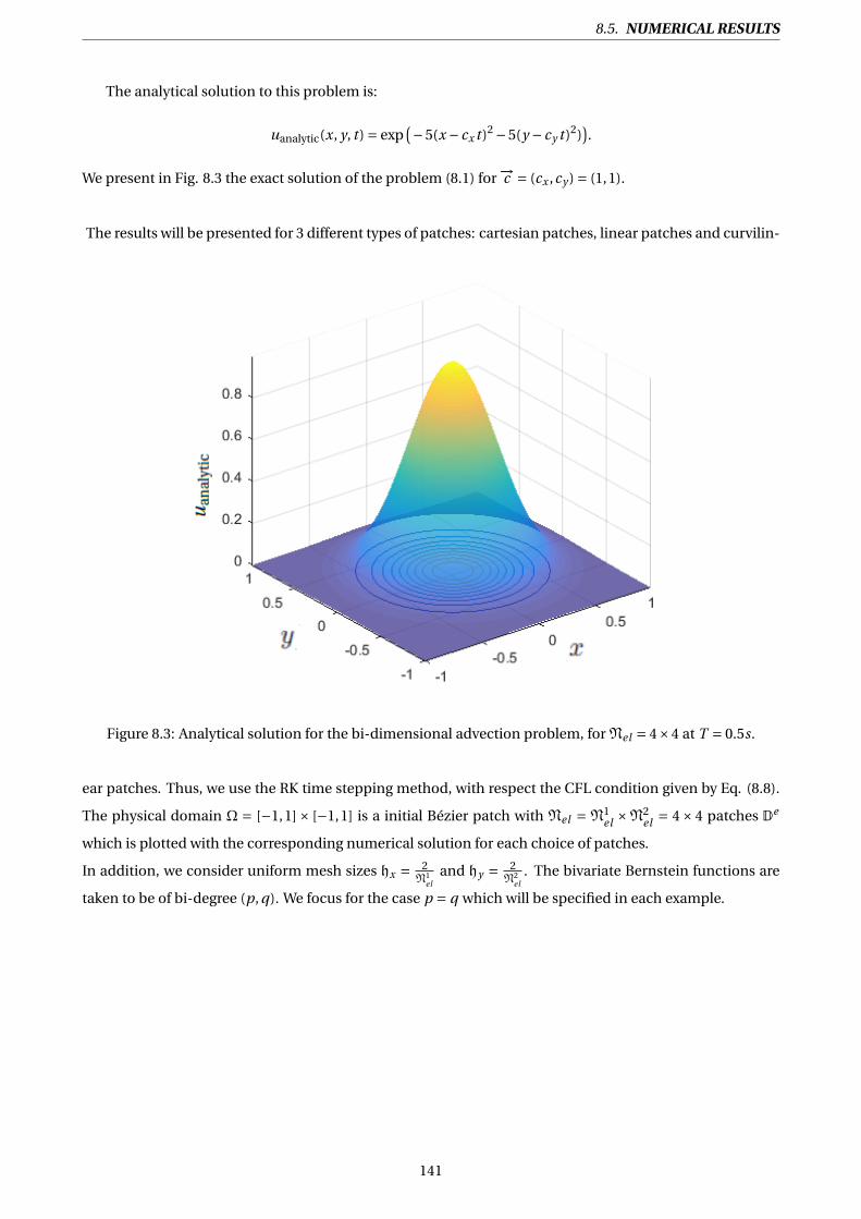
8.5. NUMERICAL RESULTS
The analytical solution to this problem is:
uanalytic(x, y, t ) = exp(−5(x − cx t )2 −5(y − cy t )2)
).
We present in Fig. 8.3 the exact solution of the problem (8.1) for −→c = (cx ,cy ) = (1,1).
The results will be presented for 3 different types of patches: cartesian patches, linear patches and curvilin-
Figure 8.3: Analytical solution for the bi-dimensional advection problem, for Nel = 4×4 at T = 0.5s.
ear patches. Thus, we use the RK time stepping method, with respect the CFL condition given by Eq. (8.8).
The physical domain Ω = [−1,1]× [−1,1] is a initial Bézier patch with Nel = N1el ×N2
el = 4× 4 patches De
which is plotted with the corresponding numerical solution for each choice of patches.
In addition, we consider uniform mesh sizes hx = 2N1
eland hy = 2
N2el
. The bivariate Bernstein functions are
taken to be of bi-degree (p, q). We focus for the case p = q which will be specified in each example.
141

CHAPTER 8. IGDG: 2D ADVECTION PROBLEM
8.5.1 Cartesian grids
The first mesh type considered are simple cartesian grids. Figure 8.4 depicts the IGDG numerical solu-
tions for the bivariate quadratic Bernstein case for the initial mesh with Nel = 4×4 patches which is plotted
in the top of Fig. 8.4. We subsequently add a reffinement of h2 as shown in the bottom of Fig. 8.4.
Figure 8.4: Plots and contour plots of numerical results for bivariate quadratic Bernstein basis with (a)Nel =4×4 patches and (b) Nel = 8×8 patches at T = 0.05s.
142

8.5. NUMERICAL RESULTS
Figure 8.5 shows the numerical solutions from IGDG space discretization and explicit RK 4 time integra-
tion for the linear, quadratic, cubic and quartic Bernstein cases. We can see the effect of the degree elevation
of the bivariate Bernstein basis function on the accuracy.
Figure 8.5: IGDG solution for Nel = 8×8 patches for different degrees (p, q).
143

CHAPTER 8. IGDG: 2D ADVECTION PROBLEM
Before we proceed further, let us recall that we denote by ∥ u ∥L2(Ω), the L2(Ω)-norm of a function u:
∥ u ∥L2(Ω)=(∫Ω
u2dΩ) 1
2.
We measure the convergence of the numerical methods in the L2-norm for the Cartesian, linear and curvi-
linear grids. Our aim is to identify the numerical order of convergence. We define the error of the numerical
solution as:
eh = uh −uex , (8.10)
and its L2-norm is:
∥ eh ∥L2(Ω) =(∫Ω
(uh(x, y)−uex (x, y)
)2dΩ)1/2
. (8.11)
Tab. 8.1 and Tab. 8.2 summarize the convergence results in the L2−norm for the bivariate linear,quadratic,
cubic and quartic Bernstein basis functions, from which we can see that the L2-convergence rate is approx-
imately p +1.
Mesh L2 −error rateh 2.235E −01 −h2 1.012E −01 1.14h4 2.586E −02 1.96h8 5.807E −03 2.15
Mesh L2 −error rateh 1.136E −01 −h2 1.476E −02 2.94h4 1.713E −03 3.10h8 2.047E −04 3.06
Table 8.1: L2−error for the 2D advection problem and convergence order for the IGDG method for the linear(left) and quadratic (right) Bernstein bases in conjunction with RK 4 time discretisation.
Mesh L2 −error rateh 3.170E −02 −h2 5.090E −03 2.63h4 2.6488E −04 4.26h8 1.650E −05 4.00
Mesh L2 −error rateh 1.706E −02 −h2 3.639E −04 5.55h4 9.763E −06 5.22h8 2.851E −07 5.09
Table 8.2: L2−error for the 2D advection problem and convergence order for the IGDG method for the cubic(left) and quartic (right) Bernstein bases in conjunction with RK 4 time discretisation.
144

8.5. NUMERICAL RESULTS
The corresponding convergence data for uniform refinement h2 , h
4 and h8 are shown in Fig. 8.6. The con-
vergence rates of the L2-norm of the error are shown in the legend.
Figure 8.6: L2−error for the 2D advection problem using the IGDG method in conjunction with RK 4.
We consider p = q ∈ 1,2,3,4 and asses the quality of numerical approximations through the L2−norm.
Table 8.1 and table 8.2 show the error of numerical approximations in L2−norm for various size of element
h and order of basis p. Those results are depicted in Figure 8.6. We obtain the convergence rates r = p +1,
p ∈ 1,2,3,4.
145

CHAPTER 8. IGDG: 2D ADVECTION PROBLEM
8.5.2 Linear grids
Linear patches are still employed in this case. The initial configurations of Nel =N1el ×N2
el patches and
degrees (p, q) of bivariate Bernstein function are the same with those described in the previous case.
Figure 8.7: Contour plots of numerical results for bivariate quadratic Bernstein basis at T = 0.05s.
146

8.5. NUMERICAL RESULTS
We refer to Figure 8.8 for comparisons of bases functions for the bivariate linear, quadratic, cubic and
quartic Bernstein functions, our mesh is a Bézier patch with Nel = 8×8 elements.
Figure 8.8: IGDG solutions for different degrees for Nel = 8×8 uniform elements.
147

CHAPTER 8. IGDG: 2D ADVECTION PROBLEM
Convergence results for the 2D advection problem with different choices of Nel are given in Tab. (8.3)
for the linear and quadratic Bernstein and in Tab. (8.4) for the cubic and quartic Bernstein.
Mesh L2 −error rateh 2.248E −01 −h2 1.043E −01 1.10h4 2.931E −02 1.83h8 6.818E −03 2.10
Mesh L2 −error rateh 1.222E −01 −h2 2.220E −02 2.46h4 3.410E −03 2.70h8 3.874E −04 3.13
Table 8.3: L2−error for the 2D advection problem and convergence order for the IGDG method for the linear(left) and quadratic (right) Bernstein bases in conjunction with RK 4 time discretisation.
Mesh L2 −error rateh 4.397E −02 −h2 5.362E −03 3.03h4 3.473E −04 3.94h8 1.915E −05 4.18
Mesh L2 −error rateh 1.845E −02 −h2 8.373E −04 4.46h4 2.871E −05 4.86h8 7.553E −07 5.19
Table 8.4: L2−error for the 2D advection problem and convergence order for the IGDG method for the cubic(left) and quartic (right) Bernstein bases in conjunction with RK 4 time discretisation.
Figure 8.9: L2−error for the 2D advection problem using the IGDG method in conjunction with RK 4.
148

8.5. NUMERICAL RESULTS
8.5.3 Curvilinear grids
In this case, we considerNel curvilinear patches. Contrary to the previous cases, the geometry curvature
is taken into account here. We underline that the boundary geometry is identically maintained whatever the
basis degree (except for p = 1) and d.o.f number.
Figure 8.10: Contour plots of numerical results for bivariate quadratic Bernstein basis at T = 0.05s.
149

CHAPTER 8. IGDG: 2D ADVECTION PROBLEM
Figure 8.11 shows the numerical solutions from IGDG space discretization and explicit RK 4 time in-
tegration for the linear, quadratic, cubic and quartic Bernstein cases. We can see the effect of the degree
elevation of the bivariate Bernstein basis function on the accuracy.
Figure 8.11: IGDG solutions for different bivariate degrees (p, q) for Nel = 8×8.
150

8.5. NUMERICAL RESULTS
In the following we investigate the numerical order of convergence in the the L2-norm of the IGDG
discretizations, the problem is solved for several different values of bivariate Bernstein polynomial degrees
(p, p) and numbers of patches Nel . The L2-norm of the error and convergence rate are shown in Table 8.5
for the linear and quadratic case and in Table 8.6 for the cubic and quartic Bernstein.
Mesh L2 −error rateh 2.176E −01 −h2 9.935E −02 1.13h4 2.792E −02 1.83h8 6.295E −03 2.14
Mesh L2 −error rateh 1.139E −01 −h2 2.206E −02 2.36h4 3.113E −03 2.82h8 3.657E −04 3.08
Table 8.5: L2−error for the 2D advection problem and convergence order for the IGDG method for the linear(left) and quadratic (right) Bernstein bases in conjunction with RK 4 time discretisation.
Mesh L2 −error rateh 4.243E −02 −h2 4.686E −03 3.17h4 3.0617E −04 3.93h8 1.705E −05 4.16
Mesh L2 −error rateh 1.611E −02 −h2 8.272E −04 4.28h4 2.382E −05 5.11h8 6.609E −07 5.17
Table 8.6: L2−error for the 2D advection problem vs. mesh parameter and convergence order for the IGDGmethod for the cubic (left) and quartic (right) Bernstein bases in conjunction with RK 4 time discretisation.
Again, as can be seen, we obtain that the L2 convergence rate is approximately p +1.
151

CHAPTER 8. IGDG: 2D ADVECTION PROBLEM
Figure 8.12: L2−errors for the 2D advection problem using the IGDG method in conjunction with RK 4.
Table 8.5 and table 8.6 show the quality of the numerical approximations in L2 norm for various size
of element h and order of polynomial (p and q). The error of the numerical approximations is depicted in
Figure 8.12. The convergence rates are 2, 3, 4 and 5 using bases of degrees p = q = 1, p = q = 2, p = q = 3
and p = q = 4, respectively.
8.6 Conclusion
As it has been pointed out previously, we can conclude that IGDG is a powerful tool. In this chapter,
we have introduced a new analysis framework, called isogeometric discontinuous Galerkin (IGDG) method
for bi-dimensional hyperbolic problem, which is based on Bézier extraction. We have confined our atten-
tion to the development of the RK-IGDG methods for bi-dimensional advection problem. The resulting
IGDG method in conjunction with RK method is stable, high-order accurate, and highly parallelizable. The
scheme can easily handle complicated geometries and boundary conditions. The flexibility of the method
to handle different geometries and to work with different elements has been shown.
As consequence, this method can be easily formulated and implemented. Thus, the numerical behavior of
the method is evaluated and it has shown an optimal convergence rate.
152


CH
AP
TE
R
92D ACOUSTIC WAVE EQUATIONS
THe purpose of this chapter is to develope and analyze the new IGDG method, that uses the
IGA discretization concept combined with the DG technique, for solving the first-order
acoustic wave equation in 2D , modelling sound propagation phenomena. The compu-
tational domain is divided into non-overlapping sub-domains, composed of B-spline patches. The DG ap-
proach was applied on element level, each element being a Bézier patch constructed from initial B-spline
patches. The solution of the problem is approximated in every element without imposing any continuity
requirements for the discrete solution on the interfaces. Basic tests of accuracy and stability are demon-
strated, including optimal convergence rates with respect to L2−norm .
9.1 Introduction and basic theory
Acoustic equations model acoustic wave propagation in a medium. Several application fields are cov-
ered by such a model, like elastic wave propagation in the ground, or sound propagation in the air [76]. The
form itself is usually considered as a linear problem governed by the compressible linearized Euler equa-
tions, in order to describe mean flow effects on sound propagation, such as refraction.
The pressure-velocity formulation of the acoustic wave equations is expressed as a linear PDE system, in
which the acoustic pressure and velocity interact with one another to propagate waves through materials.
Let Ω ⊂ R2 be a two dimensional domain with boundary ∂Ω. On each point on ∂Ω we denote by ~n the
outward normal vector. Let T > 0 be a fixed time.
154

9.2. IGDG APPROXIMATION OF THE ACOUSTIC WAVE EQUATIONS
For (x, y, t ) ∈Ω× (0,T
), the linear acoustic wave equation can be formulated as a first–order hyperbolic
system in terms of the pressure field p and velocity field−→U = (
u,v):
∂−→U∂t +∇p = 0 (x, y, t ) ∈Ω× [0,T ],∂p∂t +∇·−→U = 0 (x, y, t ) ∈Ω× [0,T ],−→U ·−→n = 0 on ∂Ω× [0,T ].
(9.1)
Here, p represent the pressure perturbation and−→U the velocity perturbation with respect to a reference state
at rest. Moreover, the equations have been adimensionalized by assuming that the sound speed is equal to
unity.
At boundary, we assume perfect wall conditions, all waves being ideally reflected.
We supplement the system (9.1) with the initial condition:u(x, y,0) = u0(x, y) (x, y) ∈Ω,
v(x, y,0) = v0(x, y) (x, y) ∈Ω,
p(x, y,0) = p0(x, y) (x, y) ∈Ω.
(9.2)
An equivalent formulation of the system (9.1) is the following:
∂u∂t +
∂p∂x = 0 (x, y, t ) ∈Ω× [0,T ], (1)
∂v∂t +
∂p∂y = 0 (x, y, t ) ∈Ω× [0,T ], (2)
∂p∂t + ∂u
∂x + ∂v∂y = 0 (x, y, t ) ∈Ω× [0,T ], (3)
−→U ·−→n = 0 on ∂Ω× [0,T ].
(9.3)
9.2 IGDG approximation of the acoustic wave equations
9.2.1 Spatial discretization
This section introduces the weak formulation of the linear acoustic wave equations given above by equa-
tion (9.3) using IGDG method. As highlighted in the previous chapter, in DG method the basis functions are
allowed to be discontinuous at the element boundaries, the integrals are performed element-wise, and the
compling of the wave field across the elements is weakly imposed using fluxes. The first step is to derive the
weak formulations of equation (9.3). This weak formulation is then discretized by introducing an approxi-
mation for the pressure and velocity in a finite-dimensional subspace to obtain a linear system of ordinary
differential equations.
155

CHAPTER 9. 2D ACOUSTIC WAVE EQUATIONS
In order to apply the IGA methodology, we highlight that the physical domain Ω is subdivided into B-
spline patches De ,
S (Ω) := DeNpa
e=1 .
We suppose that the computational domainΩ can be exactly represented by the union of non-overlapping
patches De :
Ω=⋃D
ewith
D
e ⋂ D
l
=; ∀ e 6= l .
Each patch De defined by:
De =
X e = (xe , ye ) ∈R2 | X e =T(ξ,η) such that (ξ,η) ∈ De
,
where the transformation T is defined for all (ξ,η) ∈ De by:
T : De 7−→ De
(ξ,η) 7−→ (xe (ξ,η), ye (ξ,η)
).
As in the previous chapter, a set of Bézier elements is obtained from the B-spline patches by multiple
knot insertion. Within each element De we assume that the local solution is well approximated by two-
dimensional Bernstein polynomials of degrees p and q :
uh(x, y, t )
vh(x, y, t )
ph(x, y, t )
e
=p+1∑i=1
q+1∑j=1
(Φ
p,qi , j (x, y)
)e
ui j (t )
vi j (t )
pi j (t )
e
=p+1∑i=1
q+1∑j=1
(B
p,qi , j (x, y)
)e
ui j (t )
vi j (t )
pi j (t )
e
=p+1∑i=1
q+1∑j=1
(B
p,qi , j (T(ξ,η))
)e
ui j (t )
vi j (t )
pi j (t )
e
=p+1∑i=1
q+1∑j=1
(Bi ,p (ξ)
)e(B j ,q (η)
)e
ui j (t )
vi j (t )
pi j (t )
e
where uei j : [0,T ] 7−→R, ve
i j : [0,T ] 7−→R and pei j : [0,T ] 7−→R, ∀1 ≤ i ≤ p +1, ∀1 ≤ j ≤ q +1 are local unknown
coefficients.
156

9.2. IGDG APPROXIMATION OF THE ACOUSTIC WAVE EQUATIONS
The number of degree of freedom inside the element De is (p + 1)× (q + 1).(Φ
p,qi , j
)eare the bivariate
Bernstein polynomials of degree p ×q . The global solution can then be approximated by the direct sum of
the local solutions:
u(x, y, t )
v(x, y, t )
p(x, y, t )
'
uh(x, y, t )
vh(x, y, t )
ph(x, y, t )
=Nel⊕e=1
uh(x, y, t )
vh(x, y, t )
ph(x, y, t )
e
.
Before we proceed further, let us put weh ∈Vp
h , the approximate solution will be sought for each t ∈ [0,T ] in
the finite-dimensional space:
Vph =
w := w
(x(ξ,η), y(ξ,η)
) ∈ L2(Ω), w|De ∈ spanB e,
where B e is the set of (p +1)× (q +1) Bernstein polynomials defined over De .
The starting point for a DG discretization is the weak formulation, which is obtained by multiplying each
equations of the system (9.3) by a local arbitrary test function we (x, y) ∈ Vp , and then integrating on each
Bézier patch De separately. Note that, in this framework, no continuity on the state vectors ue ,ve ,pe and
the test function we is enforced along the interfaces between Bézier patches. The weak formulation of the
acoustic wave equation is given for e = 1, ...,Nel for each equations of the system (9.3) by the following
statement:
9.2.2 First variational equation
Applying a IGDG method to equation (1) of the system (9.4), the weak form of the problem can be written
for each element De as:∫De
(∂t ue (x, y, t )+∂x pe (x, y, t )
)we (x, y)dDe = 0. (9.4)
By applying Green’s formula, the weak formulation can be written as:
∂
∂t
∫De
ue (x, y, t )we (x, y)dDe +∫Γe
pe (x, y, t )
0
·−→n e we (x, y)dΓe −∫De
pe (x, y, t )
0
·∇we (x, y)dDe = 0.
We denote: −→e x = 1
0
and −→n e the outer unit normal to Γe of the element De , so we get:
∂
∂t
∫De
ue (x, y, t )we (x, y)dDe =∫De
pe (x, y, t )−→e x ·∇we (x, y)dDe −∫Γe
pe (x, y, t )−→e x ·−→n e we (x, y)dΓe .
157

CHAPTER 9. 2D ACOUSTIC WAVE EQUATIONS
By discretizing the problem on the Bézier basis associated with the element and using Bek,l as test func-
tion, the problem is written:
p+1∑i=1
q+1∑j=1
∂t uei , j (t )
(∫DeBe
i , j (x, y)Bek,l (x, y)dDe
)=
p+1∑i=1
q+1∑j=1
pei , j (t )
(∫DeBe
i , j (x, y)−→e x ·∇Bek,l (x, y)dDe
)−
∫ΓeBe
k,l (x, y)(−→e x pe
)·−→n e dΓe
∀1 ≤ k ≤ p +1,∀1 ≤ l ≤ q +1.
Therefore, the local problem takes the form of a linear system of size (p+1)2×(q+1)2, which can be written
in the following matrix form:
Me∂t ue = Rex pe −F e
x ∀t ∈ [0,T ], ∀1 ≤ e ≤Nel . (9.5)
9.2.3 Second variational equation
In the same way, the weak form of the equation (2) of the system (9.4) can be described for each element
De as follows:∫De
(∂t ve (x, y, t )+∂y pe (x, y, t )
)we (x, y)dDe = 0. (9.6)
By applying Green’s formula, the weak formulation can be written as:
∂
∂t
∫De
ve (x, y, t )we (x, y)dDe +∫Γe
0
pe (x, y, t )
·−→n e we (x, y)dΓe −∫De
0
pe (x, y, t )
·∇we (x, y)dDe = 0.
We denote: −→e y = 0
1
, so we get:
∂
∂t
∫De
ve (x, y, t )we (x, y)dDe =∫De
pe (x, y, t )−→e y ·∇we (x, y)dDe −∫Γe
pe (x, y, t )−→e y ·−→n e we (x, y)dΓe .
By discretizing the problem on the Bézier basis associated with the element and using Bek,l as test function,
the problem is written:
p+1∑i=1
q+1∑j=1
∂t vei , j (t )
(∫DeBe
i , j (x, y)Bek,l (x, y)dDe
)=
p+1∑i=1
q+1∑j=1
pei , j (t )
(∫DeBe
i , j (x, y)−→e y ·∇Bek,l (x, y)dDe
)−
∫ΓeBe
k,l (x, y)(−→e y pe
)·−→n e dΓe ,
∀1 ≤ k ≤ p +1, ∀1 ≤ l ≤ q +1.
158

9.2. IGDG APPROXIMATION OF THE ACOUSTIC WAVE EQUATIONS
Therefore, the local problem takes the form of a linear system of size (p + 1)2 × (q + 1)2, which can be
written in the following matrix form:
Me∂t ve = Rey pe −F e
y ∀t ∈ [0,T ], ∀1 ≤ e ≤Nel . (9.7)
9.2.4 Third variational equation
In order to write the last variational equation of the system (9.4), we multiply the equation (3) with the
test function we and integrate over De :∫De
(∂t pe (x, y, t )+∂x ue (x, y, t )+∂y ve (x, y, t )
)we (x, y)dDe = 0. (9.8)
By applying Green’s formula, the weak formulation can be written as:
∂
∂t
∫De
pe (x, y, t )we (x, y)dDe +∫Γe
ue (x, y, t )
ve (x, y, t )
·−→n e we (x, y)dDe −∫De
ue (x, y, t )
ve (x, y, t )
·∇we (x, y)dDe = 0.
so we get:
∂
∂t
∫De
pe (x, y, t )we (x, y)dDe =∫De
(ue (x, y, t )−→e x +ve (x, y, t )−→e y
)·∇we (x, y)dDe
−∫Γe
(ue (x, y, t )−→e x +ve (x, y, t )−→e y
)·−→n e we (x, y)dΓe .
By discretizing the problem on the Bézier basis associated with the element and using Bek,l as test function,
the problem is written:
p+1∑i=1
q+1∑j=1
∂t pei , j (t )
(∫DeBe
i , j (x, y)Bek,l (x, y)dDe
)=
p+1∑i=1
q+1∑j=1
(ue
i , j (t )−→e x +vei , j (t )−→e y
)(∫DeBe
i , j (x, y) ·∇Bek,l (x, y)dDe
)−
∫ΓeBe
k,l (x, y)(−→e x ue +−→e y ve
)·−→n e dΓe ,
∀1 ≤ k ≤ p +1, ∀1 ≤ l ≤ q +1.
Therefore, this local problem leads to a linear system of size (p +1)2 × (q +1)2, which can be written in the
following matrix form:
Me∂t pe = Rex ue +Re
y pe − (F e
x +F ey
) ∀t ∈ [0,T ] ∀1 ≤ e ≤Nel . (9.9)
159

CHAPTER 9. 2D ACOUSTIC WAVE EQUATIONS
9.3 Elementary linear system
The coefficients of the local mass and stiffness matrix for the element De are written as:
Mekl ,i j =
∫DeBe
i , j (x, y)Bek,l (x, y)dDe
=∫DeBe
i , j (T(ξ,η))Bek,l (T(ξ,η))dDe .
By performing the integration in the local parametric space De , we get:
Mekl ,i j =
∫De
((Bi ,p (ξ)
)e(B j ,q (η))e
)((Bk,p (ξ)
)e(Bl ,q (η))e
)| J e (ξ,η) | dDe ,
∀i ,k = 1, ..., p +1, j , l = 1, ..., q +1,
where | J e | is the local Jacobien determinant defined in the previous chapter by:
| J e |=((∂x
∂ξ
)(∂y
∂η
))e −((∂x
∂η
)(∂y
∂ξ
))e.
Achieving the integration in the unit square D, we get:
Mekl ,i j =
∫D
((Bi ,p (ξ)
)e(B j ,q (η))e
)((Bk,p (ξ)
)e(Bl ,q (η))e
)| J e (ξ,η) || J e (ξ,η) | dD,
∀i ,k = 1, ..., p +1 j , l = 1, ..., q +1.
The integrals are evaluated numerically via Gaussian quadrature.
(Re
x
)kl ,i j =
∫De
(−→e xBei j (x, y)
)·∇Be
kl (x, y)dDe
=∫DeBe
i j (x, y)(∂Be
kl (x, y)
∂x
)dDe
=∫DeBe
i , j
(T(ξ,η)
) ∂∂x
Bek,l
(T(ξ,η)
)dDe ,
(Re
y
)kl ,i j =
∫De
(−→e yBei j (x, y)
)·∇Be
kl (x, y)dDe
=∫DeBe
i j (x, y)(∂Be
kl (x, y)
∂y
)dDe
=∫DeBe
i , j
(T(ξ,η)
) ∂∂y
Bek,l
(T(ξ,η)
)dDe ,
(Re)
kl ,i j = (Re
x
)kl ,i j +
(Re
y
)kl ,i j .
160

9.4. NUMERICAL LAX–FRIEDRICHS FLUXES
By expressing the integration in the local parametric space De , we get:
(Re
x
)kl ,i j =
∫De
((Bi ,p (ξ)
)e(B j ,q (η))e
)((∂B ek,p (ξ)
∂ξ
)(B e
l ,q (η)∂ξ
∂x
)+ (B e
k,p (ξ))(∂B e
l ,q (η)
∂η
∂η
∂x
))| J e (ξ,η)| dDe ,
and,
(Re
y
)kl ,i j =
∫De
((Bi ,p (ξ)
)e(B j ,q (η))e
)((∂B ek,p (ξ)
∂ξ
)(B e
l ,q (η)∂ξ
∂y
)+ (B e
k,p (ξ))(∂B e
l ,q (η)
∂η
∂η
∂y
))| J e (ξ,η)| dDe .
By performing the integration in the reference square D, we get:
(Re
x
)kl ,i j =
∫D
((Bi ,p (ξ)
)e(B j ,q (η))e
)((∂B ek,p (ξ)
∂ξ
)(B e
l ,q (η)∂ξ
∂x
)+ (B e
k,p (ξ))(∂B e
l ,q (η)
∂η
∂η
∂x
))| J e (ξ, η)| | J e (ξ,η)| dD,
(Re
y
)kl ,i j =
∫D
((Bi ,p (ξ)
)e(B j ,q (η))e
)((∂B ek,p (ξ)
∂ξ
)(B e
l ,q (η)∂ξ
∂y
)+ (B e
k,p (ξ))(∂B e
l ,q (η)
∂η
∂η
∂y
))| J e (ξ, η)| | J e (ξ,η)| dD.
At the end, the computation is achieved using Gauss-Legendre quadrature rules.
9.4 Numerical Lax–Friedrichs fluxes
The selection of the numerical flux is of utmost importance when formulating a DG method. The nu-
merical flux must accurately couple the neighboring elements, while yielding a stable scheme. There are
several flux methods. In our formulation, we only discuss the Lax-Friedrich flux [73], given by:
f en (ul ,ur ) = 1
2
(fn(ue
l )+ fn(uer )
)− ρ
2
(ue
r −uel
), (9.10)
where ul and ur are the left and right limits of the discontinuous solution uh . For the Lax-Friedrichs flux,
ρ is taken as an upper bound for | f ′(u) | in the scalar case, or for the absolute value of eigenvalues of the
Jacobian for the system case. For the acoustic wave equation, ρ is the sound speed assumed ρ = 1.
161

CHAPTER 9. 2D ACOUSTIC WAVE EQUATIONS
Since the weak form of the DG method is written elementwise, the numerical flux between adjacent
elements must be defined. For this purpose, it is possible to write:
F e =4∑
k=1
∫Γe
k
f enB
ek,l (x, y)dΓe
k
=∫
[0,1]
f en |Γe
1
(Bk,p (ξ)
)e(Bl ,q (0)︸ ︷︷ ︸=1
)e | J e (ξ,0) || J e (ξ,0) | dξ
+∫
[0,1]
f en |Γe
2
(Bk,p (1)︸ ︷︷ ︸
=1
)e(Bl ,q (η))e | J e (1,η) || J e (1, η) | dη
+∫
[0,1]
f en |Γe
3
(Bk,p (ξ)
)e(Bl ,q (1)︸ ︷︷ ︸=1
)e | J e (ξ,1) || J e (ξ,1)dξ
+∫
[0,1]
f en |Γe
4
(Bk,p (0)︸ ︷︷ ︸
=1
)e(Bl ,q (η))e | J e (0,η) || J e (0, η)dη.
It is also necessary to define for the patch De , the normal vectors on the four interfaces Γe1, Γe
2, Γe3 and Γe
4
given by:
−→n e|Γe
1
= −→
nex |Γe
1−→ne
y |Γe1
= ∂y
∂ξ
−∂x∂ξ
e
,
−→ne |Γe
2=
−→ne
x |Γe2−→
ney |Γe
2
= ∂y
∂η
−∂x∂η
e
,
−→ne |Γe
3=
−→ne
x |Γe3−→
ney |Γe
3
= −∂y
∂ξ
∂x∂ξ
e
,
−→ne |Γe
4=
−→ne
x |Γe4−→
ney |Γe
4
= −∂y
∂η
∂x∂η
e
.
Obviously, these vectors are normalized for the computations.
162

9.5. NUMERICAL RESULTS
9.5 Numerical results
We consider the example of an ideal acoustic resonator between two cylinders solved using the acoustic
wave equation (9.3) over the physical domain Ω represented in Fig. 9.1, for which an analytical solution
exists.
Two types of computational domains are considered: a curvilinear one constructed by least squares approx-
imation and knot insertion (described in chapter 4) and a rectilinear one, that corresponds to classical grids
with straight element interfaces.
Figure 9.1: Control point lattice for quadratic rectilinear grid (on the right) and curvilinear grid (on the left).
163

CHAPTER 9. 2D ACOUSTIC WAVE EQUATIONS
Figure 9.2: Rectilinear grid on the right and curvilinear grid on the left (4×4 elements).
The initial conditions are: p|t=0 = J0(α1 + r−r1
r2−r1(α2 −α1)
),
−→U |t=0 =
(u,v
)|t=0
= (0,0).
This solution is provided where α1 = 3.8317, α2 = 10.1735 (α1 and α2: roots of J ′0 = J1) (see appendix C ) ,
r1 = 0.25, r2 = 1 and J0 the Bessel function of the first kind.
The exact solutions is given in cylindrical coordinates (r,θ) by:
pex = J0
(α1 + r−r1
r2−r1(α2 −α1)
)cos
(α2−α1r2−r1
t),
uex = J1(α1 + r−r1
r2−r1(α2 −α1)
)sin
(α2−α1r2−r1
t)
cos(θ),
vex = J1(α1 + r−r1
r2−r1(α2 −α1)
)sin
(α2−α1r2−r1
t)
sin(θ).
164

9.5. NUMERICAL RESULTS
Figure 9.3: Plots and contour plots of the exact pressure pex.
Figure 9.4: Plots and contour plots of uex.
The results will be presented for rectilinear patches and curvilinear patches. The physical defined as a B-
spline patch with Nel = N1el ×N2
el = 4× 4 patches De which is plotted with the corresponding numerical
solution for each choice of patches.
The bivariate Bernstein functions are taken to be of bi-degree (p, q). We focus for the case p = q which will
be specified in each example.
165

CHAPTER 9. 2D ACOUSTIC WAVE EQUATIONS
Figure 9.5: Plots and contour plots of vanalytic.
9.5.1 Rectilinear grids
The first mesh type considered is a simple rectilinear grid. Figure 9.7 depicts the IGDG numerical solu-
tions for the bivariate quadratic Bernstein case for the initial mesh with Nel = 4×4 patches (as shown on the
left in Fig. 9.6). We subsequently add a refinement (on the right of Fig. 9.6) of (hx2 ,
hy
2 ), the IGDG numerical
solutions are shown in Fig. 9.8.
Figure 9.6: Rectilinear patches.
As can be seen on Figures 9.7 and 9.8, the use of a rectilinear grid strongly impacts the accuracy of the
166

9.5. NUMERICAL RESULTS
solution near the boundaries of the domain. In particular, one can notice the presence of fictious variations
of the solution at each boundary vertex, which are due to the fact that the boundary conditions are not pre-
scribed at the true location and normals are not well approximated. When the rectilinear grid is refined,
these effects are reduced but are still dommageable. In Figures 9.9 to 9.11, one can observe that increasing.
The approximation order of the solution only does not provide any remedy to this issue.
167

CHAPTER 9. 2D ACOUSTIC WAVE EQUATIONS
Figure 9.7: Plots and contour plots of numerical results for bivariate quadratic Bernstein basis with Nel =4×4 patches at T = 0.1s.
168

9.5. NUMERICAL RESULTS
Figure 9.8: Plots and contour plots of numerical results for bivariate quadratic Bernstein basis Nel = 8×8patches at T = 0.1s.
169

CHAPTER 9. 2D ACOUSTIC WAVE EQUATIONS
Figure 9.9, Fig. 9.10 and Fig. 9.11 shows the numerical solutions from IGDG space discretization and
explicit RK 4 time integration for the quadratic, cubic and quatric Bernstein cases respectively. We can see
the effect of the degree elevation of the bivariate Bernstein basis function on the accuracy.
Figure 9.9: IGDG solution u for different degrees p for Nel = 4×4 elements at T = 0.1s.
170

9.5. NUMERICAL RESULTS
Figure 9.10: IGDG solution v for different degrees p for Nel = 4×4 elements at T = 0.1s.
171

CHAPTER 9. 2D ACOUSTIC WAVE EQUATIONS
Figure 9.11: IGDG solution p for different degrees p for Nel = 4×4 elements at T = 0.1s.
172

9.5. NUMERICAL RESULTS
The L2−error is now presented for rectilinear patches. Tables 9.1 and 9.2 summarize the convergence
results in the L2−norm for the bivariate quadratic, cubic and quartic Bernstein basis functions.
Mesh L2 −error rateh 1.951E −01 −h2 5.241E −02 1.89h4 7.224E −03 2.85h8 1.928E −03 1.90h
16 2.524E −04 2.93
Table 9.1: L2−error for the 2D acoustic problem and convergence order for the IGDG method for thequadratic Bernstein bases in conjunction with RK 4 time discretisation.
Mesh L2 −error rateh 1.324E −01 −h2 2.622E −02 2.33h4 6.244E −03 2.07h8 1.889E −03 1.72h
16 2.480E −04 2.92
Mesh L2 −error rateh 9.624E −02 −h2 2.579E −02 1.78h4 6.220E −03 2.05h8 1.890E −03 1.71h
16 2.474E −04 2.93
Table 9.2: L2−error for the 2D acoustic problem and convergence order for the IGDG method for the cubic(left) and quartic (right) Bernstein bases in conjunction with RK 4 time discretisation.
173

CHAPTER 9. 2D ACOUSTIC WAVE EQUATIONS
The corresponding convergence data for uniform refinement h, h2 , h
4 , h8 and h
16 are shown in Figure 9.12.
Figure 9.12: L2−error for the 2D acoustic problem using the IGDG method in conjunction with RK 4.
174

9.5. NUMERICAL RESULTS
9.5.2 Curvilinear grids
We consider now the case of curvilinear grids. Figure 9.14 depicts the IGDG numerical solutions for the
bivariate quadratic Bernstein case for the initial mesh with Nel = 4×4 patches as shown on the left in Fig.
9.13. We subsequently add a reffinement of (hx2 ,
hy
2 ) as shown on the right in Fig. 9.13.
Figure 9.13: Curvilinear patches.
Contrary to the rectilinear case, the use of curvilinear grids yields a far better accuracy of the solution near
the boundaries, as shown in figures 9.14 and 9.15. In particular, one can notice that the boundary isovalues
are correctly captured, even on the coarsest grid. Figures 9.16 to 9.18 show that the increase of the approxi-
mation order of the solution yields a more accurate solution inside the domain while preserving the bound-
ary accuracy. Note that, in this case, the circle is not exactly represented because B-spline representations
are employed, instead of NURBS. Nevertheless, this does not seem to be critical in this example.
175

CHAPTER 9. 2D ACOUSTIC WAVE EQUATIONS
Figure 9.14: Plots and contour plots of numerical results for bivariate quadratic Bernstein basis with Nel =4×4 patches at T = 0.1s.
176

9.5. NUMERICAL RESULTS
Figure 9.15: Plots and contour plots of numerical results for bivariate quadratic Bernstein basis Nel = 8×8patches at T = 0.1s.
177

CHAPTER 9. 2D ACOUSTIC WAVE EQUATIONS
Figure 9.16, Fig. 9.17 and Fig. 9.18 shows the numerical solutions from IGDG space discretization and
explicit RK 4 time integration for the quadratic, cubic and quatric Bernstein cases respectively. We can see
the effect of the degree elevation of the bivariate Bernstein basis function on the accuracy.
Figure 9.16: IGDG solution u for different degrees p for Nel = 4×4 elements at T = 0.1s.
178
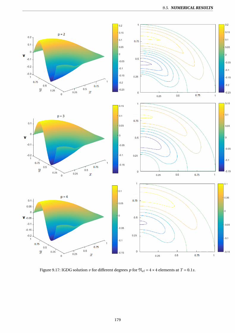
9.5. NUMERICAL RESULTS
Figure 9.17: IGDG solution v for different degrees p for Nel = 4×4 elements at T = 0.1s.
179

CHAPTER 9. 2D ACOUSTIC WAVE EQUATIONS
Figure 9.18: IGDG solution p for different degrees p for Nel = 4×4 elements at T = 0.1s.
180

9.5. NUMERICAL RESULTS
Tables 9.3 and 9.4 summarize the convergence results in the L2−norm for the bivariate quadratic, cubic
and quartic Bernstein basis functions.
Mesh L2 −error rateh 1.983E −01 −h2 4.541E −02 2.13h4 3.436E −03 3.72h8 4.066E −04 3.07h
16 5.084E −05 2.99
Table 9.3: L2−error for the 2D acoustic problem and convergence order for the IGDG method for thequadratic Bernstein bases in conjunction with RK 4 time discretisation.
Mesh L2 −error rateh 9.907E −02 −h2 2.740E −03 5.17h4 3.173E −04 3.11h8 2.019E −05 3.97h
16 1.310E −06 3.94
Mesh L2 −error rateh 1.527E −02 −h2 1.046E −03 3.86h4 2.875E −05 5.18h8 9.704E −07 4.88h
16 3.056E −08 4.98
Table 9.4: L2−error for the 2D acoustic problem and convergence order for the IGDG method for the cubic(left) and quartic (right) Bernstein bases in conjunction with RK 4 time discretisation.
The corresponding convergence data for uniform and refinement h, h2 , h
4 , h8 and h
16 are shown in Fig. 9.19.
181

CHAPTER 9. 2D ACOUSTIC WAVE EQUATIONS
Figure 9.19: L2−error for the 2D acoustic problem using the IGDG method in conjunction with RK 4.
The impact of the boundary curvature on the solution accuracy, already observed in the solution plots,
is confirmed when the convergence rates are computed. For the isogeometric approach using curvilin-
ear grids, quasi-optimal convergence rates close to order p+1 are obtained as the B-spline grids are refined.
However, when using rectilinear grids, a far lower convergence rate is observed, close to second-order (glob-
ally), whatever the degree of the solution employed (see Figure 9.12). One can even notice that the accuracy
is degraded as the degree of the solution increases, for a fixed number of degrees of freedom. The solver
tends to a solution corresponding to the uncorrect boundary geometry (location and normals). Therefore,
the use of an accurate geometry description, exact if possible, is mandatory for the efficiency of high-order
discretization schemes
9.6 Conclusion
In this chapter we gave a description of the ongoing development of a IGDG method to solve the first-
order acoustic wave equation in 2D , expressed as a linear hyperbolic PDE system. As it has been pointed out
previously, the computational domain is divided into non-overlapping sub-domains, composed of B-spline
patches. The DG approach was applied on element level, each element being a Bézier patch constructed
from initial B-spline patches. The solution of the problem is approximated in every element without any
continuity requirements for the discrete solution on the interfaces. As a result, IGDG method can be easily
formulated and implemented. Finally, the numerical behavior of the method is evaluated and it has shown
an optimal convergence rate.
182


CONCLUSION
DAns le chapitre 7, nous avons décrit les différentes procédures de calcul pour la
méthode de GD dans le cadre de l’AIG, spécialement pour le cas du problème hy-
perbolique unidimensionnel. Le présent chapitre et le chapitre précédent sont
consacrés à l’extension au cas des problèmes hyperboliques bidimensionnels. Nous avons décrit le développe-
ment d’une méthode de GD dans le cadre AIG pour résoudre l’équation d’advection en 2D dans le chapitre
précédent et le problème acoustiques de premier ordre en 2D dans le présent chapitre, qui est exprimé sous
la forme d’un système EDP linéaire hyperbolique. Comme cela a été souligné précédemment, le domaine
de calcul est divisé en sous-domaines, composés de patches B-splines. L’approche GD a été appliquée au
niveau des éléments, chaque élément étant un patch de Bézier construit à partir de patches B-splines ini-
tiaux. La solution du problème est approximée dans chaque élément sans aucune exigence de continuité
pour la solution discrète sur les interfaces. Par conséquent, la méthode de GD dans le cadre AIG peut être
facilement formulée et mise en oeuvre, elle est capable de gérer facilement des géométries complexes. La
flexibilité de la méthode pour gérer différentes géométries et pour travailler avec différents éléments a été
montrée. Ainsi, le comportement numérique de la méthode est évalué et il a été montré un taux de conver-
gence optimal selon la norme L2.
184


Part V
General Conclusion & Perspectives
186


GENERAL CONCLUSION & PERSPECTIVES
ISogeometric Analysis can be considered as a Finite Element method that general-
izes the set of basis functions from polynomials to B-splines or more generally to
non-uniform-rational B-splines. As shown in the literature, this choice guaran-
tees several advantages, from the exact parametrization of geometries defined
via CAD to a higher accuracy per-degrees-of-freedom. It also allows for solution fields with higher smooth-
ness. These reasons have made IGA a successful topic in recent years.
In this thesis we applied the IGA method to some hyperbolic problems. We considered standard
Galerkin methods as well as stabilized methods, with a special emphasis on B-splines. IGA possesses a set
of attractive features from the view point of accuracy and implementational convenience not present in
standard FE discretizations. In fact, IGA allows exact representation of a wide class of geometries even on
very coarse meshes. In particular, geometry domains having conic sections like circles, cylinders, spheres,
ellipsoids, etc... can be represented exactly using NURBS. Refinements can be performed by subdivision of
the grid (by inserting knots) or by elevation of the polynomial order of the basis functions in the same way
as using the traditional finite element method.
Due to the fact that the aim of IGA is to generalize and improve upon classical FEA, we started this thesis
by giving an introduction to IGA by revisiting the original analysis, i.e. FEA, in the context of hyperbolic PDE
with SUPG stabilization.
188

9.6. CONCLUSION
Numerical examples for advection problem were given for both classical Lagrange and B-spline bases.
It was shown that the IG method may be well suited to the hyperbolic problems if stabilization is correctly
calibrated. The convergence rates were measured in the L2−norm. The IG method was tested on different
polynomial orders. It was found that, for a given polynomial order, high regularity gives lower error versus
degrees of freedom compared to low regularity, without exceptions. Elsewhere, a possible drawback of the
SUPG method is the sensitivity of the solution to the stabilization parameter, whose optimal value is not
determined precisely by the available theory and is tedious to select in practice.
Therefore, we proposed in this thesis a new method which combines the IGA with the DG method,
called IGDG method, for solving hyperbolic problems. The major reason for using DG methods in this the-
sis lies in their ability to provide stable numerical methods for hyperbolic problems, for which classical FEM
is well known to perform poorly.
Our method takes advantage of both IGA and DG methods. In fact, DG methodology is adopted at Bézier
patch level, i.e., we employ the traditional IGA within each Bézier patch, and employ the DG method across
the patch interfaces to glue the multiple patches. Bézier patches, considered as elements, are constructed
by transformation of the initial B-spline domain (Bézier extraction is a classical CAD technique).
We consider then scalar and system of conservation laws, as test cases. These test examples show that the
resulting IGDG method in conjunction with RK method is stable, high-order accurate, and can easily han-
dle curved geometries and boundary conditions. As consequence, this method can be easily formulated
and implemented. Then, the numerical behavior of the method has been evaluated and it was shown an
optimal convergence rate for 2D advection and acoustic problems. The higher accuracy obtained by using
curvilinear elements has been demonstrated, in particular when coarse grids are employed. An accuracy
up to order five has been reached.
The present method has shown to be very effective for linear hyperbolic problems and systems in one
and two dimensions. Now, the proposed IGDG method should be extended to more complex non-linear
conservation laws, like compressible Euler equations for instance. Efficient DG methods for such non-
linear systems have been constructed recently, for classical rectilinear grids. Accounting for Bézier bases
should not exhibit specific difficulties, except for the capture of solution discontinuities that may appear
for non-linear conservation laws. In this perspective, one could extend the generalized limiters proposed
by Cockburn and coauthors (see appendix) to local Bézier representations. Another necessary extension
would concern the construction of the initial B-spline or NURBS computational domain. The geometries
considered in this work are rather simple and are represented by only one B-spline patch, before Bézier
extraction. To consider really complex geometries, a general framework to easily handle a set of B-spline
patches should be proposed. In this perspective, we underline that the proposed approach, based on DG
concepts, is more flexible that the original IGA method because no regularity constraint is necessary at the
interface between patches. Finally, one should exploit the great flexibility offered by B-spline representa-
tions in terms of p− and h− refinements in order to propose automated local refinement strategies.
189


CONCLUSION GÉNÉRALE & PERSPECTIVES
L’analyse isogéométrique peut être considérée comme une méthode par éléments fi-
nis qui généralise l’ensemble des fonctions de base pôlynomiales aux B-splines ou
plus généralement aux NURBS. Comme le montre la littérature, ce choix garantit
plusieurs avantages de la paramétrisation exacte des géométries définies par CAO à une plus grande pré-
cision par degré de liberté. Il permet également des champs de solution réguliers. Ces raisons ont fait de
l’AIG un sujet émergeant ces dernières années.
Dans cette thèse, nous avons appliqué la méthode de l’AIG à certains problèmes hyperboliques. Nous
avons considéré les méthodes standards de Galerkin ainsi que les méthodes stabilisées, en mettant partic-
ulièrement l’accent sur les B-splines. L’AIG possède un ensemble de caractéristiques attractives du point de
vue de la précision et de la commodité de mise en oeuvre qui ne sont pas présentes dans les discrétisations
d’EF standards. En fait, l’AIG permet une représentation exacte d’une large classe de géométries, même sur
des maillages très grossiers. En particulier, les domaines géométriques ayant des sections coniques comme
les cercles, les cylindres, les sphères, les ellipsoides, etc. peuvent être représentés exactement à l’aide de
NURBS. Les raffinements peuvent être effectués par subdivision de la grille (en insérant des noeuds) ou par
élévation de l’ordre polynomial des fonctions de base de la même manière que la méthode des EF tradition-
nels.
Vu que l’objectif principal de l’AIG est de généraliser et d’améliorer l’AEF classique, nous avons com-
mencé cette thèse en revisitant l’analyse originale, à savoir l’AEF, dans le contexte d’EDP hyperboliques avec
la stabilisation SUPG.
Des exemples numériques de problèmes d’advection ont été donnés pour les bases classiques de La-
grange et B-splines. Il a été montré que la méthode d’AIG peut être bien adaptée aux problèmes hyper-
boliques si la stabilisation est correctement calibrée. Les taux de convergence ont été mesurés dans la
norme standard L2. La méthode d’AIG a été testée sur différents ordres polynomiaux. On a constaté que,
pour un ordre polynomial donné, une régularité élevée donne une erreur plus faible par degré de liberté,
par rapport à une faible régularité, sans exception.
191

CHAPTER 9. 2D ACOUSTIC WAVE EQUATIONS
Par ailleurs, un inconvénient possible de la méthode SUPG est la sensibilité de la solution au paramètre
de stabilisation, dont la valeur optimale n’est pas déterminée précisément par la théorie disponible et qui
est fastidieuse à sélectionner dans la pratique.
Par conséquent, nous avons proposé dans cette thèse une nouvelle méthode qui combine l’AIG avec
la méthode de GD, appelée méthode IGDG, pour résoudre des problèmes hyperboliques. La principale rai-
son de l’utilisation des méthodes de GD dans cette thèse réside dans leur capacité à fournir des méthodes
numériques stables pour les problèmes hyperboliques, pour lesquels la MEF classique est bien connue pour
ses performances médiocres.
Notre méthode tire parti des méthodes de l’AIG et de GD. En fait, la méthodologie de GD est adoptée au
niveau des patches de Bézier, c’est-à-dire que nous utilisons l’AIG traditionnelle dans chaque patch de
Bézier et la méthode de GD sur les interfaces de patch pour assembler les multiples patches. Les patches
de Bézier, considérés comme des éléments, sont construits par transformation du domaine B-spline initial
(l’extraction de Bézier est une technique classique de CAO).
Nous considérons alors des cas scalaires et des cas systèmes de lois de conservation, comme cas tests. Ces
exemples de tests montrent que la méthode IGDG obtenue en conjonction avec la méthode de RK pour la
discrétisation temporelle est stable, de haute précision, et peut facilement gérer les géométries courbes et
les conditions aux limites. Par conséquent, cette méthode peut être facilement formulée et mise en oeu-
vre. Ainsi, le comportement numérique de la méthode a été évalué et on a montré un taux de convergence
optimal pour l’advection 2D et les problèmes acoustiques. La plus grande précision obtenue en utilisant
des éléments curvilignes a été démontrée, en particulier lorsque des grilles grossières sont utilisées. Une
précision de l’ordre de cinq a été atteinte.
La méthode actuelle s’est avérée très efficace pour les problèmes hyperboliques linéaires et les sys-
tèmes à une et deux dimensions. Maintenant, la méthode IGDG proposée devrait être étendue à des lois de
conservation non linéaires plus complexes, comme les équations d’Euler compressible, par exemple. Des
méthodes de GD efficaces pour ces systèmes non linéaires ont été construites récemment pour les grilles
rectilignes classiques. L’extension à des bases de Bézier ne devrait pas présenter de difficultés spécifiques,
sauf pour la capture des discontinuités de solution pouvant apparaître pour les lois de conservation non
linéaires. Dans cette perspective, on pourrait étendre les limiteurs généralisés proposés par Cockburn et ses
coauteurs (voir annexe) aux représentations de Bézier locales. Une autre extension nécessaire concernerait
la construction du domaine de calcul initial B-spline. Les géométries considérées dans ce travail sont plutôt
simples et représentées par un seul patch B-spline, avant l’extraction de Bézier. Pour prendre en compte des
géométries plus complexes, il convient de proposer un cadre général permettant de gérer facilement un en-
semble de patches B-spline. Dans cette perspective, nous soulignons que l’approche proposée, basée sur
les concepts GD, est plus flexible que la méthode d’AIG d’origine car aucune contrainte de régularité n’est
nécessaire à l’interface entre les patches. Enfin, il convient d’exploiter la grande flexibilité offerte par les
représentations B-splines en termes de raffinement p− et h− afin de proposer des stratégies de raffinement
locales automatisées.
192


AP
PE
ND
IX
A
A.1 Gaussian quadrature
Let Ω= [a,b] ⊂ R. A quadrature rule is defined by a set of nodes (X G (k))1≤k≤nG ∈Ω and a set of weights
(ωG (k))1≤k≤nG ∈ R. The fundamental result of Gaussian quadrature states that the optimal abscissas of the
nG -point Gaussian quadrature formulas are precisely the roots of the orthogonal polynomial for the same
interval and weighting function. Gaussian quadrature is optimal because it integrates all polynomials up to
degree 2nG −1 exactly.
WhenΩ= [−1,1], the roots of the Legendre polynomials and their corresponding weights have been exten-
sively tabulated, so we can simply use these tables without redoing the calculations.
nG Weights ωG Nodes X G
1 2 02 − 1p
3, 1p
31, 1
3 −√
35 , 0,
√35
59 , 8
9 , 59
4 −√
(15+2p
30)35 , −
√(15−2
p30)
35 ,√
(15+2p
30)35 , −
√(15−2
p30)
3518−p30
36 , 18+p3036 , 18+p30
36 , 18−p3036
Table A.1: Gauss–Legendre nodes and coefficients
We can transform any given integral on the interval [a,b] into an integral on the interval [−1,1], simply use:∫ b
af (x)d x = (b−a
2
)∫ 1
−1f( (b−a)y + (b+a)
2
)d y ≈ (b−a
2
) nG∑k=1
ωG (k) f( (b−a)X G (k)+ (b+a)
2
)
194


AP
PE
ND
IX
B
B.1 Runge-Kutta (RK) method:
The Runge-Kutta method is used to solve a system of ODEs given by:
∂t u(x, t ) =L(t ,u(x, t )
). (B.1)
The s-stage Runge-Kutta (RK) method for (B.1) is written in the form:
∂t u(1) = L(t n ,un)
∂t u(i ) = L(t n + ci∆t ,un +∆t
i−1∑j=1
ai j∂t h( j ))
i = 2, ..., s
un+1 = un +∆ts∑
i=1bi∂t u(i ),
where ∆t = t n+1 − t n is the time step, and un and un+1 represent the values of u at time t n and t n+1 respec-
tively. The coefficients ai j , bi and ci can be summarized in matrix/vector form by the Butcher tableau.
We have ai j = 0 ∀ j ≥ i . Moreover, the coefficients ci and ai j are connected by the condition:
ci =s∑
j=1ai j i = 1, ..., s.
196

B.2. 1D SLOPE LIMITING
B.2 1D slope limiting
If the solution of the problem exhibits discontinuities, the proposed scheme generates oscillations
(Gibbs phenomenon). To overcome this difficulty, a particular treatment is required, such as filtering or
limiting. In the present work, we envisage to apply the generalized limiting approach. The idea is to modify
locally the solution, if a discontinuity is detected, in order to satisfy the following conditions:
i ) Maintain the mass conservation principle in each element.
i i ) Satisfy the Total Variation Diminishing in the Means (TVDM) property.
i i i ) Do not degrade accuracy of the method.
B.2.1 TVDM limiter
The proposed approach, relies on the minmod function defined as:
m(s1, ..., sn) =
s(
mini=1,...,n
| si |)
if s = si g n(s1) = ... = si g n(sn)
0 otherwise(B.2)
Let u j denote the mean value of the solution over the elementΩ j . Thanks to the partition of unity property
of the Bézier representation, it can be simply evaluated by:
u j = 1
p +1
p+1∑i=1
uij
(n).
The minmod function is employed to extrapolate linearly the mean value u j at the element extremities,
according to a limited slope estimation, using:
ulj = u j −m
(u j −u1
j(n)
,u j+1 −u j ,u j −u j−1), (B.3)
urj = u j +m
(up+1
j
(n) −u j ,u j+1 −u j ,u j −u j−1). (B.4)
If ulj = u1
j(n)
and urj = up+1
j
(n), i.e. the local slope (first argument of the minmod function) is lower than
the slopes based on neighbors values (second and third arguments), and all slopes have the same sign, the
solution remains unchanged, because this indicates a region where the solution is regular. On the contrary,
a possible discontinuity is detected and the solution in the elementΩ j is replaced by a linear approximation
with the limited slope:
uh |Ω j(x) = u j +
( x −x j
h/2
)min(ml ,mr ),
where ml and mr denote the limited slopes computed in Eq.(B.3) and Eq.(B.4). Using a local Bernstein basis,
such a linear representation can be obtained easily be setting a linear variation of the degrees of freedom:
uij
(n) = u j +(2(i −1)
p−1
)min(ml ,mr ) i = 1, ..., p +1.
197

APPENDIX B.
B.2.2 TVBM limiter
The TVDM generalized slope limiter described above yields a loss of accuracy in the vicinity of local
extrema of the solution. To prevent this effect, one must construct a Total Variation Bounded in the Means
(TVBM) limiter, instead of the TVDM one.
This can easily be achieved by introducing a modified minmod function (less restrictive):
m(s1, ..., sn) = s1 if | s1 |≤Ch2,
m(s1, ..., sn) otherwise,
which is used in replacement of Eq. (B.2) to compute limited slopes. C should be an upper bound of the
absolute value of the second order derivative of the solution at local extrema.
198

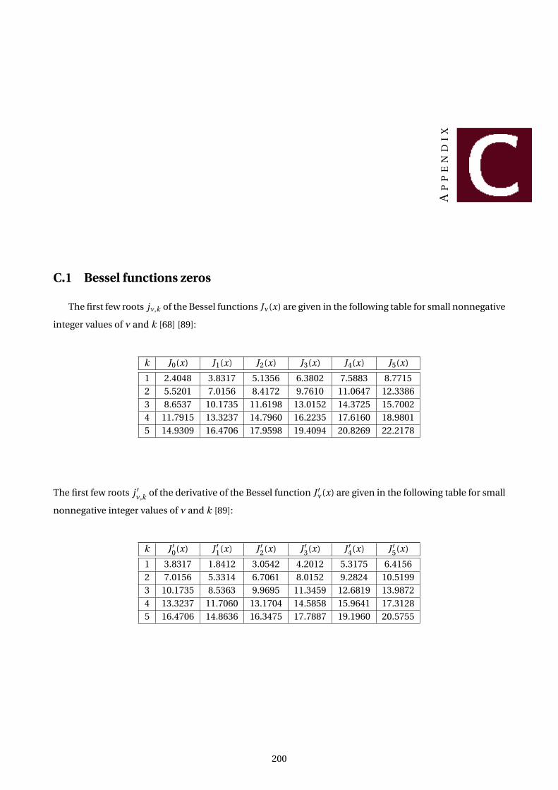
AP
PE
ND
IX
C
C.1 Bessel functions zeros
The first few roots jν,k of the Bessel functions Jν(x) are given in the following table for small nonnegative
integer values of ν and k [68] [89]:
k J0(x) J1(x) J2(x) J3(x) J4(x) J5(x)
1 2.4048 3.8317 5.1356 6.3802 7.5883 8.77152 5.5201 7.0156 8.4172 9.7610 11.0647 12.33863 8.6537 10.1735 11.6198 13.0152 14.3725 15.70024 11.7915 13.3237 14.7960 16.2235 17.6160 18.98015 14.9309 16.4706 17.9598 19.4094 20.8269 22.2178
The first few roots j ′ν,k of the derivative of the Bessel function J ′ν(x) are given in the following table for small
nonnegative integer values of ν and k [89]:
k J ′0(x) J ′1(x) J ′2(x) J ′3(x) J ′4(x) J ′5(x)
1 3.8317 1.8412 3.0542 4.2012 5.3175 6.41562 7.0156 5.3314 6.7061 8.0152 9.2824 10.51993 10.1735 8.5363 9.9695 11.3459 12.6819 13.98724 13.3237 11.7060 13.1704 14.5858 15.9641 17.31285 16.4706 14.8636 16.3475 17.7887 19.1960 20.5755
200


BIBLIOGRAPHY
[1] J. E. Akin and T. E. Tezduyar. Calculation of the advective limit of the SUPG stabilization parameter for
linear and higher-order elements. Computer Methods in Applied Mechanics and Engineering, 193(21-
22):1909–1922, 2004.
[2] I. Akkerman, Y. Bazilevs, V. Calo, T. Hughes, and S. Hulshoff. The role of continuity in residual-based
variational multiscale modeling of turbulence. Computational Mechanics, 41(3):371–378, 2008.
[3] D. Al-Akhrass. Méthodes éléments finis mixtes robustes pour gérer l’incompressibilité en grandes défor-
mations dans un cadre industriel. PhD thesis, Ecole Nationale Supérieure des Mines de Saint-Etienne,
2014.
[4] A. B. H. Ali and A. Soulaimani. An unstructured finite elements method for solving the compressible
RANS equations and the Spalart-Allmaras turbulence model. Computer Methods in Applied Mechanics
and Engineering, 199(33-36):2261–2272, 2010.
[5] D. N. Arnold, F. Brezzi, B. Cockburn, and L. D. Marini. Unified analysis of discontinuous Galerkin
methods for elliptic problems. SIAM Journal on Numerical Analysis, 39(5):1749–1779, 2002.
[6] C. Baiocchi, F. Brezzi, and L. P. Franca. Virtual bubbles and Galerkin-least-squares type methods (GLS).
Computer Methods in Applied Mechanics and Engineering, 105(1):125–141, 1993.
[7] Y. Bazilevs, K. Takizawa, and T. E. Tezduyar. Computational fluid-structure interaction: methods and
applications. John Wiley & Sons, 2013.
[8] P. Bézier. Essai de définition numérique des courbes et des surfaces expérimentales: contribution à l’étude
des propriétés des courbes et des surfaces paramétriques polynomiales à coefficients vectoriels. PhD the-
sis, Université Pierre et Marie Curie (Paris V I ), 1977.
[9] M. Billaud. Eléments finis stabilisés pour des écoulements diphasiques compressible-incompressible.
PhD thesis, Université de Bordeaux 1, 2009.
[10] C. F. Borges and T. Pastva. Total least squares fitting of Bézier and B-spline curves to ordered data.
Computer Aided Geometric Design, 19(4):275–289, 2002.
[11] S. Brenner and R. Scott. The mathematical theory of finite element methods, volume 15. Springer
Science & Business Media, 2007.
202

BIBLIOGRAPHY
[12] F. Brezzi. On the existence, uniqueness and approximation of saddle-point problems arising from la-
grangian multipliers. Revue Française d’Automatique, Informatique, Recherche Opérationnelle. Analyse
Numérique, 8:129–151, 1974.
[13] A. N. Brooks. A Petrov-Galerkin finite element formulation for convection dominated flows. PhD thesis,
California Institute of Technology, 1981.
[14] A. N. Brooks and T. J. Hughes. Streamline Upwind/Petrov-Galerkin formulations for convection domi-
nated flows with particular emphasis on the incompressible Navier-Stokes equations. Computer Meth-
ods in Applied Mechanics and Engineering, 32(1-3):199–259, 1982.
[15] H. Carbonel, A. Carlos, A. C. Galeão, and A. D. Loula. Numerical study of Petrov-Galerkin formulations
for the shallow water wave equations. Journal of the Brazilian Society of Mechanical Sciences, 22(2):231–
247, 2000.
[16] T. H. Chien. Development of isogeometric finite element methods. PhD thesis, Vietnam National Uni-
versity - Faculty of Mathematics and Computer Science Department of Mechanics, 2015.
[17] I. Christie, D. F. Griffiths, A. R. Mitchell, and O. C. Zienkiewicz. Finite element methods for second order
differential equations with significant first derivatives. International Journal for Numerical Methods in
Engineering, 10(6):1389–1396, 1976.
[18] B. Cockburn, S. Hou, and C.-W. Shu. The Runge-Kutta local projection discontinuous Galerkin finite
element method for conservation laws. IV . The multidimensional case. Mathematics of Computation,
54(190):545–581, 1990.
[19] B. Cockburn, S.-Y. Lin, and C.-W. Shu. TVB Runge-Kutta local projection discontinuous Galerkin fi-
nite element method for conservation laws I I I : One-dimensional systems. Journal of Computational
Physics, 84(1):90–113, 1989.
[20] B. Cockburn and C.-W. Shu. The Runge-Kutta local projection P 1-discontinuous-Galerkin finite
element method for scalar conservation laws. Mathematical Modelling and Numerical Analysis,
25(3):337–361, 1991.
[21] B. Cockburn and C.-W. Shu. The Runge-Kutta discontinuous Galerkin method for conservation laws
v : multidimensional systems. Journal of Computational Physics, 141(2):199–224, 1998.
[22] B. Cockburn and C.-W. Shu. Runge-Kutta discontinuous Galerkin methods for convection-dominated
problems. Journal of Scientific Computing, 16(3):173–261, 2001.
[23] J. A. Cottrell, T. J. Hughes, and Y. Bazilevs. Isogeometric analysis: toward integration of CAD and FEA.
John Wiley & Sons, 2009.
[24] J. A. Cottrell, A. Reali, Y. Bazilevs, and T. J. Hughes. Isogeometric analysis of structural vibrations. Com-
puter Methods in Applied Mechanics and Engineering, 195(41-43):5257–5296, 2006.
203

BIBLIOGRAPHY
[25] G. Dattoli and A. Torre. Theory and applications of generalized Bessel functions. Aracne Rome, 1996.
[26] K. David. Multi-patch Discontinuous Galerkin isogeometric analysis for porous media flow. PhD thesis,
2017.
[27] C. De Boor. On calculating with B-splines. Journal of Approximation Theory, 6(1):50–62, 1972.
[28] D. A. Di Pietro and A. Ern. Mathematical aspects of discontinuous Galerkin methods, volume 69.
Springer Science & Business Media, 2011.
[29] M. S. Floater. Derivatives of rational Bézier curves. Computer Aided Geometric Design, 9(3):161–174,
1992.
[30] L. P. Franca, S. L. Frey, and T. J. Hughes. Stabilized finite element methods: I . Application to the
advective-diffusive model. Computer Methods in Applied Mechanics and Engineering, 95(2):253–276,
1992.
[31] L. P. Franca, G. Hauke, and A. Masud. Revisiting stabilized finite element methods for the advective-
diffusive equation. Computer Methods in Applied Mechanics and Engineering, 195(13-16):1560–1572,
2006.
[32] T.-P. Fries and H. G. Matthies. A review of Petrov-Galerkin stabilization approaches and an extension
to meshfree methods. Technische Universitat Braunschweig, Brunswick, 2004.
[33] A. Gdhami, R. Duvigneau, and M. Moakher. Méthode de Galerkin discontinue: Cas de l’analyse
isogéométrique. In TAM-TAM 2017-Tendances dans les Applications Mathématiques en Tunisie, Algérie
et Maroc, 2017.
[34] S. Gottlieb and C.-W. Shu. Total variation diminishing Runge-Kutta schemes. Mathematics of Compu-
tation of the American Mathematical Society, 67(221):73–85, 1998.
[35] D. Griffiths and J. Lorenz. An analysis of the Petrov—Galerkin finite element method. Computer Meth-
ods in Applied Mechanics and Engineering, 14(1):39–64, 1978.
[36] J.-L. Guermond and R. Pasquetti. A correction technique for the dispersive effects of mass lumping for
transport problems. Computer Methods in Applied Mechanics and Engineering, 253:186–198, 2013.
[37] S. Hall, M. Eaton, and M. Williams. The application of isogeometric analysis to the neutron diffusion
equation for a pincell problem with an analytic benchmark. Annals of Nuclear Energy, 49:160–169,
2012.
[38] J. Heinrich, P. Huyakorn, O. Zienkiewicz, and A. Mitchell. An "upwind" finite element scheme for two-
dimensional convective transport equation. International Journal for Numerical Methods in Engineer-
ing, 11(1):131–143, 1977.
204

BIBLIOGRAPHY
[39] J. S. Hesthaven and T. Warburton. Nodal discontinuous Galerkin methods: algorithms, analysis, and
applications. Springer Science & Business Media, 2007.
[40] C. Hofer and U. Langer. Dual-primal isogeometric tearing and interconnecting solvers for large-scale
systems of multipatch continuous Galerkin IgA equations. ArXiv preprint arXiv:1511.07183, 2015.
[41] T. Hughes and T. Tezduyar. Development of time-accurate finite element techniques for first order
hyperbolic systems with emphasys on the compressible Euler equations. Computer Methods in Applied
Mechanics and Engineering, 45(1-3):217–284, 1984.
[42] T. J. Hughes. A simple scheme for developing ‘upwind’ finite elements. International Journal for Nu-
merical Methods in Engineering, 12(9):1359–1365, 1978.
[43] T. J. Hughes, J. A. Cottrell, and Y. Bazilevs. Isogeometric analysis: CAD, finite elements, NURBS, exact
geometry and mesh refinement. Computer Methods in Applied Mechanics and Engineering, 194(39-
41):4135–4195, 2005.
[44] T. J. Hughes, L. P. Franca, and M. Balestra. A new finite element formulation for computational fluid dy-
namics: v . Circumventing the Babuška-Brezzi condition: A stable Petrov-Galerkin formulation of the
Stokes problem accommodating equal-order interpolations. Computer Methods in Applied Mechanics
and Engineering, 59(1):85–99, 1986.
[45] T. J. Hughes and T. Tezduyar. Finite element methods for first-order hyperbolic systems with particular
emphasis on the compressible Euler equations. Computer Methods in Applied Mechanics and Engi-
neering, 45(1-3):217–284, 1984.
[46] N. Jaxon and X. Qian. Isogeometric analysis on triangulations. Computer-Aided Design, 46:45–57, 2014.
[47] V. John and P. Knobloch. On spurious oscillations at layers diminishing (SOLD) methods for
convection-diffusion equations: Part I -A review. Computer Methods in Applied Mechanics and En-
gineering, 196(17-20):2197–2215, 2007.
[48] V. John and P. Knobloch. On spurious oscillations at layers diminishing (SOLD) methods for
convection-diffusion equations: Part I I -Analysis for P 1 and Q1 finite elements. Computer Methods
in Applied Mechanics and Engineering, 197(21-24):1997–2014, 2008.
[49] C. Johnson, U. Nävert, and J. Pitkäranta. Finite element methods for linear hyperbolic problems. Com-
puter Methods in Applied Mechanics and Engineering, 45(1-3):285–312, 1984.
[50] R. Kelisky and T. Rivlin. Iterates of Bérnstein polynomials. Pacific Journal of Mathematics, 21(3):511–
520, 1967.
[51] D. Kelly, S. Nakazawa, O. Zienkiewicz, and J. Heinrich. A note on upwinding and anisotropic balancing
dissipation in finite element approximations to convective diffusion problems. International Journal
for Numerical Methods in Engineering, 15(11):1705–1711, 1980.
205

BIBLIOGRAPHY
[52] T. Krarup. A contribution to the mathematical foundation of physical geodesy. Geod. Inst. Copenhagen,
Medd., No. 44, 80 p., 44, 1969.
[53] P. Lancaster and K. Salkauskas. Surfaces generated by moving least squares methods. Mathematics of
Computation, 37(155):141–158, 1981.
[54] U. Langer and I. Toulopoulos. Analysis of multipatch discontinuous Galerkin IgA approximations to
elliptic boundary value problems. Computing and Visualization in Science, 17(5):217–233, 2015.
[55] B.-G. Lee and Y. Park. Approximate conversion of rational Bézier curves. J. KSIAM, 2:88–93, 1998.
[56] R. J. LeVeque. Finite volume methods for hyperbolic problems, volume 31. Cambridge University Press,
2002.
[57] K. J. Liew, A. Ramli, and A. A. Majid. B-spline surface fitting on scattered points. Applied Mathematics
& Information Sciences, 10(1):273, 2016.
[58] J. Liou and T. E. Tezduyar. Finite element solution techniques for large-scale problems in compu-
tational fluid dynamics. Technical, Department of Mechanical Engineering University of Houston,
Houston, TX 77004, 1987.
[59] H. Liu and K. Xu. A Runge-Kutta discontinuous Galerkin method for viscous flow equations. Journal
of Computational Physics, 224(2):1223–1242, 2007.
[60] S. May. Splines for damage and fracture in solids. PhD thesis, University of Glasgow, 2016.
[61] C. Michoski, J. Chan, L. Engvall, and J. A. Evans. Foundations of the blended isogeometric discontinu-
ous Galerkin (BIDG) method. Computer Methods in Applied Mechanics and Engineering, 305:658–681,
2016.
[62] S. J. Miller. The method of least squares. Mathematics Department Brown University, 8:1–7, 2006.
[63] A. Mizukami and T. J. Hughes. A Petrov-Galerkin finite element method for convection-dominated
flows: an accurate upwinding technique for satisfying the maximum principle. Computer Methods in
Applied Mechanics and Engineering, 50(2):181–193, 1985.
[64] K. W. Morton and D. F. Mayers. Numerical solution of partial differential equations: an introduction.
Cambridge University Press, 2005.
[65] E. Nava-Yazdani and K. Polthier. De Casteljaus algorithm on manifolds. Computer Aided Geometric
Design, 30(7):722–732, 2013.
[66] T. N. Nguyen. Isogeometric Finite Element Analysis based on Bézier Extraction of NURBS and T-
Splines. Master’s thesis, NTNU- Norwegian University of Science and Technology, 2011.
[67] K. Nguyen Tan. Surfaces polyédriques et surfaces paramétriques: une reconstruction par approximation
via les surfaces de subdivision. PhD thesis, Aix-Marseille 2, 2010.
206

BIBLIOGRAPHY
[68] J. Niedziela. Bessel functions and their applications. University of Tennessee-Knoxville, 2008.
[69] A. Owens, J. Welch, J. Kópházi, and M. D. Eaton. Discontinuous isogeometric analysis methods for the
first-order form of the neutron transport equation with discrete ordinate (SN) angular discretisation.
Journal of Computational Physics, 315:501–535, 2016.
[70] Y. Park and N. Lee. Application of degree reduction of polynomial Bézier curves to rational case. Journal
of Applied Mathematics and Computing, 18(1-2):159, 2005.
[71] J. Proft and B. Rivière. Analytical and numerical study of diffusive fluxes for transport equations with
near-degenerate coefficients. University of Pittsburgh Report, 2007.
[72] J. Proft and B. Riviere. Discontinuous Gelerkin methods for convection-diffusion equations for varying
and vanishing diffusivity. International Journal of Numerical Analysis & Modeling, 6(4), 2009.
[73] J. Qiu, B. C. Khoo, and C.-W. Shu. A numerical study for the performance of the Runge-Kutta dis-
continuous Galerkin method based on different numerical fluxes. Journal of Computational Physics,
212(2):540–565, 2006.
[74] W. H. Reed and T. Hill. Triangular mesh methods for the neutron transport equation. Technical report,
Los Alamos Scientific Lab., N. Mex.(USA), 1973.
[75] D. Régis. An introduction to isogeometric analysis with application to thermal conduction. Thème
numérique 6957, INRIA, Juin 2009.
[76] S. W. Rienstra and A. Hirschberg. An introduction to acoustics. Eindhoven University of Technology,
18:19, 2003.
[77] S. H. M. Roth. Bernstein-Bézier representations for facial surgery simulation, volume 16. ETH Zurich,
2002.
[78] F. Shakib, T. J. Hughes, and Z. Johan. A new finite element formulation for computational fluid dynam-
ics: x. the compressible Euler and Navier-Stokes equations. Computer Methods in Applied Mechanics
and Engineering, 89(1-3):141–219, 1991.
[79] C.-W. Shu. Discontinuous Galerkin methods: general approach and stability. Division of Applied Math-
ematics, Brown University, 44, 2009.
[80] C.-W. Shu and S. Osher. Efficient implementation of essentially non-oscillatory shock-capturing
schemes. Journal of Computational Physics, 77(2):439–471, 1988.
[81] E. Süli. Lecture notes on finite element methods for partial differential equations. Mathematical Insti-
tute, University of Oxford, 2012.
[82] T. Tezduyar and D. Ganjoo. Petrov-Galerkin formulations with weighting functions dependent upon
spatial and temporal discretization: Applications to transient convection-diffusion problems. Com-
puter Methods in Applied Mechanics and Engineering, 59(1):49–71, 1986.
207
BIBLIOGRAPHY
[83] T. Tezduyar and T. Hughes. Finite element formulations for convection dominated flows with particular
emphasis on the compressible Euler equations. In 21st Aerospace Sciences Meeting, page 125, 1983.
[84] T. E. Tezduyar. Computation of moving boundaries and interfaces and stabilization parameters. Inter-
national Journal for Numerical Methods in Fluids, 43(5):555–575, 2003.
[85] T. E. Tezduyar, S. Mittal, S. Ray, and R. Shih. Incompressible flow computations with stabilized bi-
linear and linear equal-order-interpolation velocity-pressure elements. Computer Methods in Applied
Mechanics and Engineering, 95(2):221–242, 1992.
[86] T. E. Tezduyar and Y. Osawa. Finite element stabilization parameters computed from element matrices
and vectors. Computer Methods in Applied Mechanics and Engineering, 190(3-4):411–430, 2000.
[87] T. Toulorge. Efficient Runge-Kutta discontinuous Galerkin methods applied to aeroacoustics. KU Leu-
ven, Departement Werktuigkunde, Leuven, 2012.
[88] L. N. Trefethen. Finite difference and spectral methods for ordinary and partial differential equations,
volume 299. Cornell University-Department of Computer Science and Center for Applied Mathemat-
ics, 1996.
[89] G. N. Watson. A treatise on the theory of Bessel functions. Cambridge University Press, 1995.
[90] E. Wendland and H. Schulz. Numerical experiments on mass lumping for the advection-diffusion
equation. Revista Minerva, 2(2):227–233, 2005.
[91] C. Wervaecke. Simulation d’écoulements turbulents compressibles par une méthode d’éléments finis
stabilisée. PhD thesis, University of Bordeaux 1, 2010.
[92] G. Xu, B. Mourrain, R. Duvigneau, and A. Galligo. Parameterization of computational domain in isogeo-
metric analysis: methods and comparison. Computer Methods in Applied Mechanics and Engineering,
200(23-24):2021–2031, 2011.
[93] Q. Xu and J. S. Hesthaven. Discontinuous Galerkin method for fractional convection-diffusion equa-
tions. SIAM Journal on Numerical Analysis, 52(1):405–423, 2014.
[94] B. Yazid. Etude des courbes de Bézier et des B-splines. Master’s thesis, Université Ahmed Ben Bella
d’Oran 1, Es Senia, 2011.
[95] F. Zhang, Y. Xu, and F. Chen. Discontinuous Galerkin methods for isogeometric analysis for elliptic
equations on surfaces. Communications in Mathematics and Statistics, 2(3-4):431–461, 2014.
[96] L. Zhang, T. Gu, J. Zhao, S. Ji, M. Hu, and X. Li. An improved moving least squares method for curve
and surface fitting. Mathematical Problems in Engineering, 2013.
208


![DIFFERENTIAL INVARIANTS OF GENERIC HYPERBOLIC MONGE… · 2017-11-07 · arXiv:nlin/0604038v1 [nlin.SI] 19 Apr 2006 DIFFERENTIAL INVARIANTS OF GENERIC HYPERBOLIC MONGE–AMPERE EQUATIONS`](https://static.documents.pub/doc/80x56/5e5cbc6b0d2e9359b01d2e6a/differential-invariants-of-generic-hyperbolic-monge-2017-11-07-arxivnlin0604038v1.jpg)
