

KLU–A HIGH PERFORMANCE SPARSE LINEAR SOLVERFOR CIRCUIT SIMULATION PROBLEMS
By
EKANATHAN PALAMADAI NATARAJAN
A THESIS PRESENTED TO THE GRADUATE SCHOOLOF THE UNIVERSITY OF FLORIDA IN PARTIAL FULFILLMENT
OF THE REQUIREMENTS FOR THE DEGREE OFMASTER OF SCIENCE
UNIVERSITY OF FLORIDA
2005

Copyright 2005
by
Ekanathan Palamadai Natarajan

I dedicate this work to my mother Savitri who has been a source of inspiration
and support to me.

ACKNOWLEDGMENTS
I would like to thank Dr. Timothy Davis, my advisor for introducing me
to the area of sparse matrix algorithms and linear solvers. I started only with
my background in numerical analysis and algorithms, a year and half back. The
insights and knowledge I have gained since then in the area and in implementing
a sparse linear solver like KLU would not have been possible but for Dr. Davis’
guidance and help. I thank him for giving me an opportunity to work on KLU. I
would like to thank Dr. Jose Fortes and Dr. Arunava Banerjee for their support
and help and for serving on my committee.
I would like to thank CISE administrative staff for helping me at different
times during my master’s research work.
iv

TABLE OF CONTENTSpage
ACKNOWLEDGMENTS . . . . . . . . . . . . . . . . . . . . . . . . . . . . . iv
LIST OF TABLES . . . . . . . . . . . . . . . . . . . . . . . . . . . . . . . . . vii
LIST OF FIGURES . . . . . . . . . . . . . . . . . . . . . . . . . . . . . . . . viii
ABSTRACT . . . . . . . . . . . . . . . . . . . . . . . . . . . . . . . . . . . . ix
CHAPTER
1 INTRODUCTION . . . . . . . . . . . . . . . . . . . . . . . . . . . . . . 1
2 THEORY: SPARSE LU . . . . . . . . . . . . . . . . . . . . . . . . . . . 5
2.1 Dense LU . . . . . . . . . . . . . . . . . . . . . . . . . . . . . . . 52.2 Sparse LU . . . . . . . . . . . . . . . . . . . . . . . . . . . . . . . 72.3 Left Looking Gaussian Elimination . . . . . . . . . . . . . . . . . 82.4 Gilbert-Peierls’ Algorithm . . . . . . . . . . . . . . . . . . . . . . 10
2.4.1 Symbolic Analysis . . . . . . . . . . . . . . . . . . . . . . . 112.4.2 Numerical Factorization . . . . . . . . . . . . . . . . . . . . 13
2.5 Maximum Transversal . . . . . . . . . . . . . . . . . . . . . . . . 142.6 Block Triangular Form . . . . . . . . . . . . . . . . . . . . . . . . 162.7 Symmetric Pruning . . . . . . . . . . . . . . . . . . . . . . . . . . 182.8 Ordering . . . . . . . . . . . . . . . . . . . . . . . . . . . . . . . . 192.9 Pivoting . . . . . . . . . . . . . . . . . . . . . . . . . . . . . . . . 222.10 Scaling . . . . . . . . . . . . . . . . . . . . . . . . . . . . . . . . . 232.11 Growth Factor . . . . . . . . . . . . . . . . . . . . . . . . . . . . . 252.12 Condition Number . . . . . . . . . . . . . . . . . . . . . . . . . . 272.13 Depth First Search . . . . . . . . . . . . . . . . . . . . . . . . . . 302.14 Memory Fragmentation . . . . . . . . . . . . . . . . . . . . . . . . 312.15 Complex Number Support . . . . . . . . . . . . . . . . . . . . . . 332.16 Parallelism in KLU . . . . . . . . . . . . . . . . . . . . . . . . . . 33
3 CIRCUIT SIMULATION: APPLICATION OF KLU . . . . . . . . . . . 35
3.1 Characteristics of Circuit Matrices . . . . . . . . . . . . . . . . . . 373.2 Linear Systems in Circuit Simulation . . . . . . . . . . . . . . . . 383.3 Performance Benchmarks . . . . . . . . . . . . . . . . . . . . . . . 393.4 Analyses and Findings . . . . . . . . . . . . . . . . . . . . . . . . 413.5 Alternate Ordering Experiments . . . . . . . . . . . . . . . . . . . 42
v
3.6 Experiments with UF Sparse Matrix Collection . . . . . . . . . . 443.6.1 Different Ordering Schemes in KLU . . . . . . . . . . . . . 443.6.2 Timing Different Phases in KLU . . . . . . . . . . . . . . . 453.6.3 Ordering Quality among KLU, UMFPACK and Gilbert-
Peierls . . . . . . . . . . . . . . . . . . . . . . . . . . . . 453.6.4 Performance Comparison between KLU and UMFPACK . . 48
4 USER GUIDE FOR KLU . . . . . . . . . . . . . . . . . . . . . . . . . . 51
4.1 The Primary KLU Structures . . . . . . . . . . . . . . . . . . . . 514.1.1 klu common . . . . . . . . . . . . . . . . . . . . . . . . . . 514.1.2 klu symbolic . . . . . . . . . . . . . . . . . . . . . . . . . . 534.1.3 klu numeric . . . . . . . . . . . . . . . . . . . . . . . . . . 55
4.2 KLU Routines . . . . . . . . . . . . . . . . . . . . . . . . . . . . . 584.2.1 klu analyze . . . . . . . . . . . . . . . . . . . . . . . . . . . 584.2.2 klu analyze given . . . . . . . . . . . . . . . . . . . . . . . 594.2.3 klu *factor . . . . . . . . . . . . . . . . . . . . . . . . . . . 594.2.4 klu *solve . . . . . . . . . . . . . . . . . . . . . . . . . . . 604.2.5 klu *tsolve . . . . . . . . . . . . . . . . . . . . . . . . . . . 614.2.6 klu *refactor . . . . . . . . . . . . . . . . . . . . . . . . . . 624.2.7 klu defaults . . . . . . . . . . . . . . . . . . . . . . . . . . 634.2.8 klu *rec pivot growth . . . . . . . . . . . . . . . . . . . . . 634.2.9 klu *estimate cond number . . . . . . . . . . . . . . . . . . 644.2.10 klu free symbolic . . . . . . . . . . . . . . . . . . . . . . . 654.2.11 klu free numeric . . . . . . . . . . . . . . . . . . . . . . . . 66
REFERENCES . . . . . . . . . . . . . . . . . . . . . . . . . . . . . . . . . . . 67
BIOGRAPHICAL SKETCH . . . . . . . . . . . . . . . . . . . . . . . . . . . . 69
vi
LIST OF TABLESTable page
3–1 Comparison between KLU and SuperLU on overall time and fill-in . . 39
3–2 Comparison between KLU and SuperLU on factor time and solve time 40
3–3 Ordering results using BTF+AMD in KLU on circuit matrices . . . . 41
3–4 Comparison of ordering results produced by BTF+AMD, AMD, MMD 43
3–5 Fill-in with four different schemes in KLU . . . . . . . . . . . . . . . . 46
3–6 Time in seconds, spent in different phases in KLU . . . . . . . . . . . 47
3–7 Fill-in among KLU, UMFPACK and Gilbert-Peierls . . . . . . . . . . 49
3–8 Performance comparison between KLU and UMFPACK . . . . . . . . 50
vii

LIST OF FIGURESFigure page
2–1 Nonzero pattern of x when solving Lx = b . . . . . . . . . . . . . . . 13
2–2 A matrix permuted to BTF form . . . . . . . . . . . . . . . . . . . . 16
2–3 A symmetric pruning scenario . . . . . . . . . . . . . . . . . . . . . . 18
2–4 A symmetric matrix and its graph representation . . . . . . . . . . . 21
2–5 The matrix and its graph representation after one step of Gaussianelimination . . . . . . . . . . . . . . . . . . . . . . . . . . . . . . . 21
2–6 A doubly bordered block diagonal matrix and its corresponding ver-tex separator tree . . . . . . . . . . . . . . . . . . . . . . . . . . . . 34
viii

Abstract of Thesis Presented to the Graduate Schoolof the University of Florida in Partial Fulfillment of the
Requirements for the Degree of Master of Science
KLU–A HIGH PERFORMANCE SPARSE LINEAR SOLVERFOR CIRCUIT SIMULATION PROBLEMS
By
Ekanathan Palamadai Natarajan
August 2005
Chair: Dr. Timothy A. DavisMajor Department: Computer and Information Science and Engineering
The thesis work focuses on KLU, a sparse high performance linear solver for
circuit simulation matrices. During the circuit simulation process, one of the key
steps is to solve sparse systems of linear equations of very high order. KLU targets
solving these systems with efficient ordering mechanisms and high performance
factorization and solve algorithms. KLU uses a hybrid ordering strategy that
comprises an unsymmetric permutation to ensure zero free diagonal, a symmetric
permutation to block upper triangular form and a fill reducing ordering such as
approximate minimum degree.
The factorization is based on Gilbert-Peierls’ left-looking algorithm with
partial pivoting. KLU also includes features like symmetric pruning to cut down
symbolic analysis costs. It offers to solve up to four right hand sides in a single
solve step. In addition, it offers transpose and conjugate transpose solve capabili-
ties and important diagnostic features to estimate the reciprocal pivot growth of
the factorization and condition number of the input matrix.
The algorithm is implemented in the C language with MATLAB interfaces as
well. The MATLAB interfaces enable a user to invoke KLU routines from within
ix

the MATLAB environment. The implementation was tested on circuit matrices
and the results determined. KLU achieves superior fill-in quality with its hybrid
ordering strategy and achieves a good performance speed-up when compared with
existing sparse linear solvers for circuit problems. The thesis highlights the work
being done on exploiting parallelism in KLU as well.
x

CHAPTER 1INTRODUCTION
Sparse is beautiful. Solving systems of linear equations of the form Ax = b
is a fundamental and important area of high performance computing. The matrix
A is called the coefficient matrix and b the right hand side vector. The vector x is
the solution to the equation. There are a number of methods available for solving
such systems. Some of the popular ones are Gaussian elimination, QR factorization
using Householder transformations or Givens rotations and Cholesky factorization.
Gaussian elimination with partial pivoting is the most widely used algorithm for
solving linear systems because of its stability and better time complexity. Cholesky
can be used only when A is symmetric positive definite.
Some systems that are solved comprise a dense coefficient matrix A. By dense,
we mean most of the elements in A are nonzero. There are high performance
subroutines such as the BLAS [1, 2, 3, 4, 5] that can maximize flop count for
such dense matrices. The interesting systems are those where the coefficient
matrix A happens to be sparse. By sparse, we mean the matrix has few nonzero
entries(hereafter referred to simply as ’nonzeros’). The adjective ’few’ is not well-
defined as we will see in chapter two. When matrices tend to be sparse, we need
to find out effective ways to store the matrix in memory since we want to avoid
storing zeros of the matrix. When we store only the nonzeros in the matrix, it has
consequences in the factorization algorithm as well. One typical example would be
we do not know before hand how nonzeros would appear in the L and U factors
when we factorize the matrix. While we avoid storing the zeros, we also want to
achieve good time complexity when solving sparse systems. If the time spent to
1

2
solve sparse systems remains same as for dense systems, we have not done any
better.
KLU stands for Clark Kent LU, since it is based on Gilbert-Peierls’ algorithm,
a non-supernodal algorithm, which is the predecessor to SuperLU, a supernodal
algorithm. KLU is a sparse high performance linear solver that employs hybrid
ordering mechanisms and elegant factorization and solve algorithms. It achieves
high quality fill-in rate and beats many existing solvers in run time, when used for
matrices arising in circuit simulation.
There are several flavours of Gaussian elimination. A left-looking Gaussian
elimination algorithm factorizes the matrix left to right computing columns of L
and U. A right-looking version factorizes the matrix from top-left to bottom-right
computing column of L and row of U. Both have their advantages and disad-
vantages. KLU uses a left looking algorithm called Gilbert-Peierls’ algorithm.
Gilbert-Peierls’ comprises a graph theoretical symbolic analysis phase that iden-
tifies the nonzero pattern of each column of L and U factors and a left-looking
numerical factorization phase with partial pivoting that calculates the numerical
values of the factors. KLU uses Symmetric Pruning to cut down symbolic analysis
cost. We shall look in detail on these features in chapter two.
A critical issue in linear solvers is Ordering. Ordering means permuting the
rows and columns of a matrix, so that the fill-in in the L and U factors is reduced
to a minimum. A fill-in is defined as a nonzero appearing in either of the matrices
L or U, while the element in the corresponding position in A is a zero. Lij or Uij
is a fill-in if Aij is a zero. Fill-in has obvious consequences in memory in that
the factorization algorithm could create dense L and U factors that can exhaust
available memory. A good ordering algorithm yields a low fill-in in the factors.
Finding the ordering that gives minimal fill-in is an NP complete problem. So
3
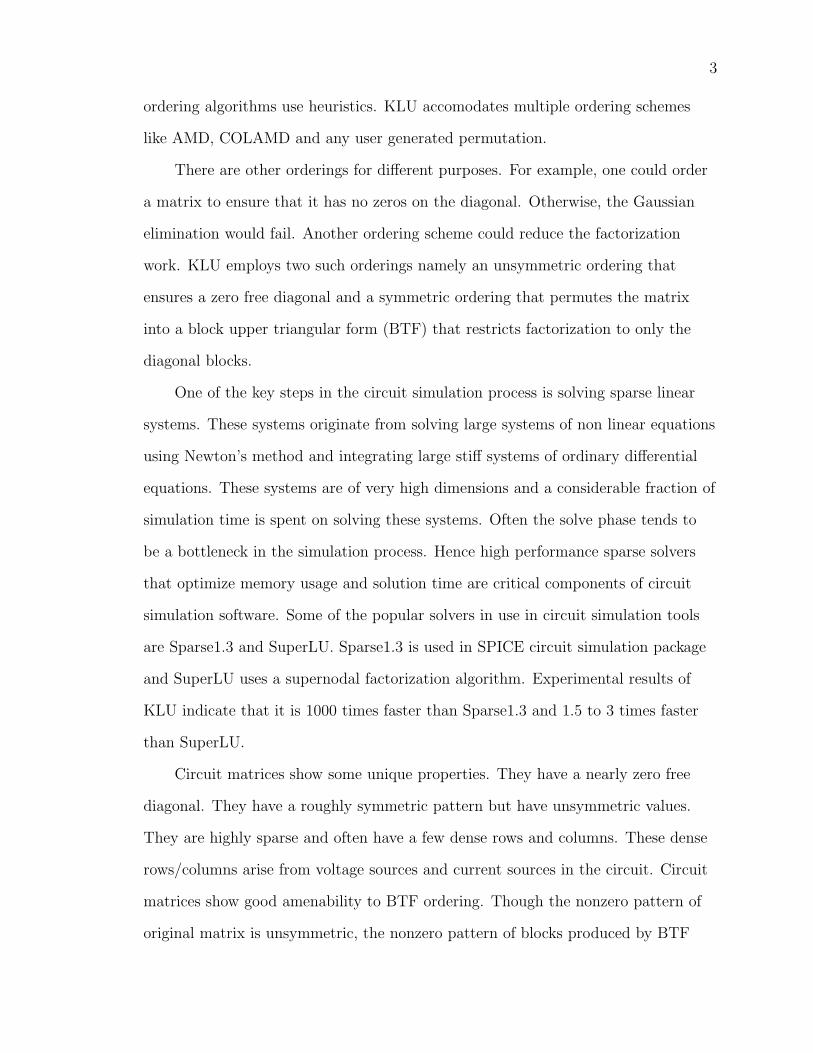
ordering algorithms use heuristics. KLU accomodates multiple ordering schemes
like AMD, COLAMD and any user generated permutation.
There are other orderings for different purposes. For example, one could order
a matrix to ensure that it has no zeros on the diagonal. Otherwise, the Gaussian
elimination would fail. Another ordering scheme could reduce the factorization
work. KLU employs two such orderings namely an unsymmetric ordering that
ensures a zero free diagonal and a symmetric ordering that permutes the matrix
into a block upper triangular form (BTF) that restricts factorization to only the
diagonal blocks.
One of the key steps in the circuit simulation process is solving sparse linear
systems. These systems originate from solving large systems of non linear equations
using Newton’s method and integrating large stiff systems of ordinary differential
equations. These systems are of very high dimensions and a considerable fraction of
simulation time is spent on solving these systems. Often the solve phase tends to
be a bottleneck in the simulation process. Hence high performance sparse solvers
that optimize memory usage and solution time are critical components of circuit
simulation software. Some of the popular solvers in use in circuit simulation tools
are Sparse1.3 and SuperLU. Sparse1.3 is used in SPICE circuit simulation package
and SuperLU uses a supernodal factorization algorithm. Experimental results of
KLU indicate that it is 1000 times faster than Sparse1.3 and 1.5 to 3 times faster
than SuperLU.
Circuit matrices show some unique properties. They have a nearly zero free
diagonal. They have a roughly symmetric pattern but have unsymmetric values.
They are highly sparse and often have a few dense rows and columns. These dense
rows/columns arise from voltage sources and current sources in the circuit. Circuit
matrices show good amenability to BTF ordering. Though the nonzero pattern of
original matrix is unsymmetric, the nonzero pattern of blocks produced by BTF

4
ordering tend to be symmetric. Since circuit matrices are extremely sparse, sparse
matrix algorithms such as SuperLU [6] and UMFPACK [7, 8] that employ dense
BLAS kernels are often inappropriate. Another unique characteristic of circuit
matrices is that employing a good ordering strategy keeps the L and U factors
sparse. However as we will see in experimental results, typical ordering strategies
can lead to high fill-in.
In circuit simulation problems, typically the circuit matrix template is gen-
erated once and the numerical values of the matrix alone change. In other words,
the nonzero pattern of the matrix does not change. This implies that we need
to order and factor the matrix once to generate the ordering permutations and
the nonzero patterns of L and U factors. For all subsequent matrices, we can use
the same information and need only to recompute the numerical values of the
L and U factors. This process of skipping analysis and factor phases is called
refactorization.Refactorization leads to a significant reduction in run time.
Because of the unique characteristics of circuit matrices and their amenability
to BTF ordering, KLU is a method well-suited to circuit simulation problems. KLU
has been implemented in the C language. It offers a set of API for the analysis
phase, factor phase, solve phase and refactor phase. It also offers the ability to
solve upto four right hand sides in a single solve step. In addition, it offers trans-
pose solve, conjugate transpose solve features and diagnostic tools like pivot growth
estimator and condition number estimator. It also offers a MATLAB interface for
the API so that KLU can be used from within the MATLAB environment.

CHAPTER 2THEORY: SPARSE LU
2.1 Dense LU
Consider the problem of solving the linear system of n equations in n un-
knowns:
a11x1 + a12x2 + ...+ a1nxn = b1
a21x1 + a22x2 + ...+ a2nxn = b2
... (2–1)
an1x1 + an2x2 + ...+ annxn = bn
or, in matrix notation,
a11 a12 · · · a1n
a21 a22 · · · a2n
...
an1 an2 · · · ann
∗
x1
x2
...
xn
=
b1
b2
...
bn
(2–2)
Ax = b
where A = (aij), x = (x1, x2, ..., xn)T and b = (b1, ..., bn)T . A well-known approach
to solving this equation is Gaussian elimination. Gaussian elimination consists of a
series of eliminations of unknowns xi from the original system. Let us briefly review
the elimination process. In the first step, the first equation of 2–1 is multiplied
by −a21
a11,−a31
a11, ... − an1
a11and added with the second through nth equation of 2–1
respectively. This would eliminate x1 from second through the nth equations. After
5

6
the first step, the 2–2 would become
a11 a12 · · · a1n
0 a(1)22 · · · a
(1)2n
...
0 a(1)n2 · · · a
(1)nn
∗
x1
x2
...
xn
=
b1
b(1)2
...
b(1)n
(2–3)
where a(1)22 = a22 − a21
a11∗ a12, a32(1) = a32 − a31
a11∗ a12 and so on. In the second
step, x2 will be eliminated by a similar process of computing multipliers and adding
the multiplied second equation with the third through nth equations. After n-1
eliminations, the matrix A is transformed to an upper triangular matrix U . The
upper triangular system is then solved by back-substitution.
An equivalent interpretation of this elimination process is that we have
factorized A into a lower triangular matrix L and an upper triangular matrix U
where
L =
1 0 0 · · · 0
a21
a111 0 · · · 0
a31
a11
a(1)32
a(1)22
1 · · · 0
...
an1
a11
a(1)n2
a(1)22
a(2)n3
a(2)33
· · · 1
(2–4)
and
U =
a11 a12 a13 · · · a1n
0 a(1)22 a23(1) · · · a
(1)2n
0 0 a33(2) · · · a(2)3n
...
0 0 0 · · · a(n−1)nn
(2–5)
The column k of the lower triangular matrix L consists of the multipliers
obtained during step k of the elimination process, with their sign negated.
7
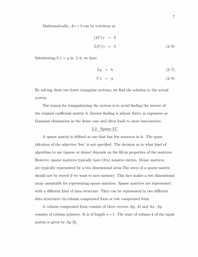
Mathematically, Ax = b can be rewritten as
(LU)x = b
L(Ux) = b (2–6)
Substituting Ux = y in 2–6, we have
Ly = b (2–7)
Ux = y (2–8)
By solving these two lower triangular systems, we find the solution to the actual
system.
The reason for triangularizing the system is to avoid finding the inverse of
the original coefficient matrix A. Inverse finding is atleast thrice as expensive as
Gaussian elimination in the dense case and often leads to more inaccuracies.
2.2 Sparse LU
A sparse matrix is defined as one that has few nonzeros in it. The quan-
tification of the adjective ’few’ is not specified. The decision as to what kind of
algorithm to use (sparse or dense) depends on the fill-in properties of the matrices.
However, sparse matrices typically have O(n) nonzero entries. Dense matrices
are typically represented by a two dimensional array.The zeros of a sparse matrix
should not be stored if we want to save memory. This fact makes a two dimensional
array unsuitable for representing sparse matrices. Sparse matrices are represented
with a different kind of data structure. They can be represented in two different
data structures viz.column compressed form or row compressed form.
A column compressed form consists of three vectors Ap, Ai and Ax. Ap
consists of column pointers. It is of length n+1. The start of column k of the input
matrix is given by Ap [k].

8
Ai consists of row indices of the elements. This is a zero based data structure
with row indices in the interval [0,n). Ax consists of the actual numerical values of
the elements.
Thus the elements of a column k of the matrix are held in
Ax [Ap [k]...Ap [k+1]). The corresponding row indices are held in
Ai [Ap [k]...Ap[k+1]).
Equivalently, a row compressed format stores a row pointer vector Ap, a
column indices vector Ai and a value vector Ax. For example, the matrix
5 0 0
4 2 0
3 1 8
when represented in column compressed format will be
Ap: 0 3 5 6
Ai: 0 1 2 1 2 2
Ax: 5 4 3 2 1 8
and when represented in row compressed format will be
Ap: 0 1 3 6
Ai: 0 0 1 0 1 2
Ax: 5 4 2 3 1 8
Let nnz represent the number of nonzeros in a matrix of dimension n ∗ n.
Then in a dense matrix representation, we will need n2 memory to represent the
matrix. In sparse matrix representation, we reduce it to O(n + nnz) and typically
nnz � n2.
2.3 Left Looking Gaussian Elimination
Let us derive a left looking version of Gaussian elimination. Let an input
matrix A of order n ∗ n be represented as a product of two triangular matrices L
and U.
9
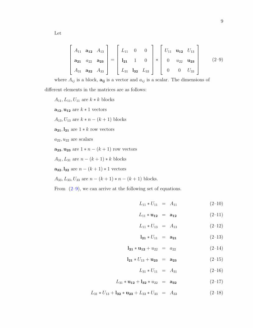
Let
A11 a12 A13
a21 a22 a23
A31 a32 A33
=
L11 0 0
l21 1 0
L31 l32 L33
∗
U11 u12 U13
0 u22 u23
0 0 U33
(2–9)
where Aij is a block, aij is a vector and aij is a scalar. The dimensions of
different elements in the matrices are as follows:
A11, L11, U11 are k ∗ k blocks
a12,u12 are k ∗ 1 vectors
A13, U13 are k ∗ n− (k + 1) blocks
a21, l21 are 1 ∗ k row vectors
a22, u22 are scalars
a23,u23 are 1 ∗ n− (k + 1) row vectors
A31, L31 are n− (k + 1) ∗ k blocks
a32, l32 are n− (k + 1) ∗ 1 vectors
A33, L33, U33 are n− (k + 1) ∗ n− (k + 1) blocks.
From (2–9), we can arrive at the following set of equations.
L11 ∗ U11 = A11 (2–10)
L11 ∗ u12 = a12 (2–11)
L11 ∗ U13 = A13 (2–12)
l21 ∗ U11 = a21 (2–13)
l21 ∗ u12 + u22 = a22 (2–14)
l21 ∗ U13 + u23 = a23 (2–15)
L31 ∗ U11 = A31 (2–16)
L31 ∗ u12 + l32 ∗ u22 = a32 (2–17)
L31 ∗ U13 + l32 ∗ u23 + L33 ∗ U33 = A33 (2–18)

10
From (2–11), (2–14) and (2–17), we can compute the 2nd column of L
and U, assuming we have already computed L11, l21 and L31. We first solve the
lower triangular system (2–11) for u12. Then, we solve for u22 using (2–14) by
computing the sparse dot product
u22 = a22 − l21 ∗ u12 (2–19)
Finally we solve (2–17) for l32 as
l32 =1
u22
(a32 − L31 ∗ u12) (2–20)
This step of computing the 2nd column of L and U can be considered equiva-
lent to solving a lower triangular system as follows:
L11 0 0
l21 1 0
L31 0 1
∗
u12
u22
l32 ∗ u22
=
a12
a22
a32
(2–21)
This mechanism of computing column k of L and U by solving a lower
triangular system L ∗ x = b is the key step in a left-looking factorization algorithm.
As we will see later, Gilbert-Peierls’ algorithm revolves around solving this lower
triangular system. The algorithm is called a left-looking algorithm since column
k of L and U are computed by using the already computed columns 1...k-1 of L.
In other words, to compute column k of L and U, one looks only at the already
computed columns 1...k-1 in L, that are to the left of the currently computed
column k.
2.4 Gilbert-Peierls’ Algorithm
Gilbert-Peierls’ [9] proposed an algorithm for Gaussian elimination with partial
pivoting in time proportional to the flop count of the elimination to factor an
arbitrary non singular sparse matrix A as PA = LU . If flops(LU) is the number

11
of nonzero multiplications performed when multiplying two matrices L and U , then
Gaussian elimination uses exactly flops(LU) multiplications and divisions to factor
a matrix A into L and U . Given an input matrix and assuming no partial pivoting,
it is possible to predict the nonzero pattern of its factors. However with partial
pivoting, it is not possible to predict the exact nonzero pattern of the factors
before hand. Finding an upper bound is possible, but the bound can be very loose
[10]. Note that computing the nonzero pattern of L and U is a necessary part of
Gaussian elimination involving sparse matrices since we do not use two dimensional
arrays for representing them but sparse data structures. Gilbert-Peierls’ algorithm
aims at computing the nonzero pattern of the factors and the numerical values in a
total time proportional to O(flops(LU)).
It consists of two stages for determining every column of L and U . The first
stage is a symbolic analysis stage that computes the nonzero pattern of the column
k of the factors. The second stage is the numerical factorization stage that involves
solving the lower triangular system Lx = b, that we discussed in the section above.
2.4.1 Symbolic Analysis
A sparse Gaussian elimination algorithm with partial pivoting cannot know
the exact nonzero structure of the factors ahead of all numerical computation,
simply because partial pivoting at column k can introduce new nonzeros in columns
k+1 · · ·n. Solving Lx = b must be done in time proportional to the number of flops
performed. Consider a simple column-oriented algorithm in MATLAB notation for
solving Lx = b as follows:
x = b
for j = 1:n
if x(j) ~= 0
x(j+1:n) = x(j+1:n) - L(j+1:n,j) * x(j)
end

12
end
The above algorithm takes time O(n + number of flops performed). The O(n)
term looks harmless, but Lx = b is solved n times in the factorization of A = LU ,
leading to an unacceptable O(n2) term in the work to factorize A into L times U .
To remove the O(n) term, we must replace the algorithm with
x = b
for each j for which x(j) ~= 0
x(j+1:n) = x(j+1:n) - L(j+1:n, j) * x(j)
end
This would reduce the O(n) term to O(η(b)), where η(b) is the number of nonzeros
in b. Note that b is a column of the input matrix A. Thus to solve Lx = b, we need
to know the nonzero pattern of x before we compute x itself. Symbolic analysis
helps us determine the nonzero pattern of x.
Let us say we are computing column k of L and U . Let G = G(Lk) be
the directed graph of L with k − 1 vertices representing the already computed
k − 1 columns. G(Lk) has an edge j → i iff lij 6= 0. Let β = {i|bi 6= 0} and
X = {i|xi 6= 0} Now the elements of X is given by
X = ReachG(L)(β) (2–22)
The nonzero pattern of X is computed by the determining the vertices that
are reachable from the vertices of the set β. The reachability problem can be solved
using a classical depth first search in G(Lk) from the vertices of the set β. If bj 6= 0,
then xj 6= 0. In addition if Lij 6= 0, then xi 6= 0 even if bi = 0. This is because
a Lij ∗ xj contributes to a nonzero in the equation when we solve for xi. During
the depth first search, Gilbert-Peierls’ algorithm computes the topological order of
X. This topological ordering is useful for eliminating unknowns in the Numerical
factorization step.

13
L
xj
xilij
Figure 2–1: Nonzero pattern of x when solving Lx = b
The row indices vector Li of columns 1 · · · k − 1 of L represents the adjacency
list of the graph G(Lk). The depth first search takes time proportional to the
number of vertices examined plus the number of edges traversed.
2.4.2 Numerical Factorization
Numerical factorization consists of solving the system (2–21) for each col-
umn k of L and U . Normally we would solve for the unknowns in (2–21) in the
increasing order of the row index. The row indices/nonzero pattern computed by
depth first search are not necessarily in increasing order. Sorting the indices would
increase the time complexity above our O(flops(LU)) goal. However, the require-
ment of eliminating unknowns in increasing order can be relaxed to a topological
order of the row indices. An unknown xi can be computed, once all the unknowns
xj of which it is dependent on are computed. This is obvious when we write the
equations comprising a lower triangular solve. Theoretically, the unknowns can be
solved in any topological order. The depth first search algorithm gives one such
topological order which is sufficient for our case. In our example, the depth first
search would have finished exploring vertex i before it finishes exploring vertices j.

14
Hence a topological order given by depth first search would have j appearing before
i. This is exactly what we need.
Gilbert-Peierls’ algorithm starts with an identity L matrix. The entire left
looking algorithm can be summarized in MATLAB notation as follows:
L = I
for k = 1:n
x = L \ A(:,k)
%(partial pivoting on x can be done here)
U(1:k,k) = x(1:k)
L(k:n,k) = x(k:n) / U(k,k)
end
where x = L\b denotes the solution of a sparse lower triangular system. In
this case, b is the kth column of A. The total time complexity of Gilbert-Peierls’
algorithm is O(η(A) + flops(LU)). η(A) is the number of nonzeros in the matrix A
and flops(LU) is the flop count of the product of the matrices L and U. Typically
flops(LU) dominates the complexity and hence the claim of factorizing in time
proportional to the flop count.
2.5 Maximum Transversal
Duff [11, 12] proposed an algorithm for determining the maximum transversal
of a directed graph.The purpose of the algorithm is to find a row permutation that
minimizes the zeros on the diagonal of the matrix. For non singular matrices, the
algorithm ensures a zero free diagonal. KLU employs Duff’s [11, 12] algorithm
to find an unsymmetric permutation of the input matrix to determine a zero-
free diagonal. A matrix cannot be permuted to have a zero free diagonal if and
only if it is structurally singular. A matrix is structurally singular if there is no
permutation of its nonzero pattern that makes it numerically nonsingular.
15
A transversal is defined as a set of nonzeros, no two of which lie in the same
row or column, on the diagonal of the permuted matrix. A transversal of maximum
length is the maximum transversal.
Duff’s maximum transversal algorithm consists of representing the matrix as
a graph with each vertex corresponding to a row in the matrix. An edge ik → ik+1
exists in the graph if A(ik, jk+1) is a nonzero and A(ik+1, jk+1) is an element in the
transversal set. A path between vertices i0 and ik would consist of a sequence of
nonzeros (i0, j1), (i1, j2), · · · (ik−1, jk) where the current transversal would include
(i1, j1), (i2, j2), · · · (ik, jk). If there is a nonzero in position (ik, jk+1) and no nonzero
in row i0 or column jk+1 is currently on the travseral, it increases the transerval
by one by adding the nonzeros (ir, jr+1), r = 0, 1, · · · , k to the transversal and
removing the nonzeros (ir, jr), r = 1, 2, · · · , k from the transversal. This adding and
removing of nonzeros to and from the transversal is called reassignment chain or
augmenting path.
A vertex or row is said to be assigned if a nonzero in the row is chosen for
the transversal. The process of constructing augmenting paths is done by doing
a depth first search from an unassigned row i0 of the matrix and continue till a
vertex ik is reached where the path terminates because A(ik, jk+1) is a nonzero and
column jK+1 is unassigned. Then the search backtracks to i0 adding and removing
transversal elements thus constructing an augmenting path.
Duff’s maximum transversal transversal algorithm has a worst case time
complexity of O(nτ) where τ is the number of nonzeros in the matrix and n is the
order of the matrix. However in practice, the time complexity is close to O(n+ τ).
The maximum transversal problem can be cast as a maximal matching
problem on bipartite graphs. This is only to make a comparison. The maximal
matching problem is stated as follows.

16
0
=
A11 A13 A14
A34
A22 A23 A24
A33
A44
x1
x2
x3
x4
b1
b2
b3
b4
A12
Figure 2–2: A matrix permuted to BTF form
Given an undirected graph G = (V,E), a matching is a subset of the edges
M ⊆ E such that for all vertices v ∈ V , at most one edge of M is incident on
v. A vertex v ∈ V is matched if some edge in M is incident on v, otherwise, v is
unmatched. A maximal matching is a matching of maximum cardinality, that is a
matching M such that for any matching M ′, we have |M | ≥ |M ′|.
A maximal matching can be built incrementally, by picking an arbitraty edge e
in the graph, deleting any edge that is sharing a vertex with e and repeating until
the graph is out of edges.
2.6 Block Triangular Form
A block (upper) triangular matrix is similar to a upper triangular matrix
except that the diagonals in the former are square blocks instead of scalars. Figure
2–2 shows a matrix permuted to the BTF form.
Converting the input matrix to block triangular form is important in that,
1. The part of the matrix below the block diagonal requires no factorization
effort.
17
2. The diagonal blocks are independent of each other.Only the blocks need to
be factorized. For example, in figure 2–2, the subsystem A44x4 = b4 can be
solved independently for x4 and x4 can be eliminated from the overall system.
The system A33x3 = b3 − A34x4 is then solved for x3 and so on.
3. The off diagonal nonzeros do not contribute to any fill-in.
Finding a symmetric permutation of a matrix to its BTF form is equivalent
to finding the strongly connected components of a graph. A strongly connected
component of a directed graph G = (V,E) is a maximal set of vertices C ⊆ V such
that for every pair of vertices u and v in C, we have both u → v and v → u. The
vertices u and v are reachable from each other.
The Algorithm employed in KLU for symmetric permutation of a matrix to a
BTF form, is based on Duff and Reid’s [13, 14] algorithm. Duff and Reid provide
an implementation for Tarjan’s [15] algorithm to determine the strongly connected
components of a directed graph. The algorithm has a time complexity of O(n + τ)
where n is the order of the matrix and τ is the number of off diagonal nonzeros in
the matrix.
The algorithm essentially consists of doing a depth first search from unvisited
nodes in the graph. It uses a stack to keep track of nodes being visited and uses a
path of the nodes. When all edges in the path are explored, it generates Strongly
connected components from the top of stack.
Duff’s algorithm is different from the method proposed by Cormen, Leiserson,
Rivest and Stein [16]. They suggest doing a depth first search on G , computing GT
and then running a depth first search on GT on vertices in the decreasing order of
their finish times from the first depth first search (the topological order from the
first depth first search).

18
����
����
����
j i k
j
i
s
= Pruned, = Fill in= Nonzero,
Figure 2–3: A symmetric pruning scenario
2.7 Symmetric Pruning
Eisenstat and Liu [17] proposed a method called Symmetric Pruning to exploit
structural symmetry for cutting down the symbolic analysis time. The cost of
depth first search can be cut down by pruning unnecessary edges in the graph of
L,G(L). The idea is to replace G(L) by a reduced graph of L. Any graph H can be
used in place of G(L), provided that i→ j exists in H iff i→ j exists in G(L). If A
is symmetric, then the symmetric reduction is just the elimination tree.
The symmetric reduction is a subgraph of G(L). It has fewer edges than G(L)
and is easier to compute by taking advantage of symmetry in the structure of
the factors L and U. Even though the symmetric reduction removes edges, it still
preserves the paths between vertices of the original graph.
Figure 2–3 shows a symmetric pruning example.
If lij 6= 0, uji 6= 0, then we can prune edges j → s, where s > i. The reason
behind this is that for any ajk 6= 0, ask will fill in from column j of L for s > k.

19
The just computed column i of L is used to prune earlier columns. Any future
depth first search from vertex j will not visit vertex s, since s would have been
visited via i already.
Note that every column is pruned only once. KLU employs symmetric pruning
to speed up the depth first search in the symbolic analysis stage.
2.8 Ordering
It is a widely used practice to precede the factorization step of a sparse
linear system by an ordering phase. The purpose of the ordering is to generate a
permutation P , that reduces the fill-in in the factorization phase of PAP T . A fill-in
is defined as a nonzero in a position (i, j) of the factor that was zero in the original
matrix. In other words, we have a fill-in if Lij 6= 0, where Aij = 0.
The permuted matrix created by the ordering PAP T creates much less fill-in
in factorization phase than the unpermuted matrix A. The ordering mechanism
typically takes into account only the structure of the input matrix, without
considering the numerical values stored in the matrix. Partial pivoting during
factorization changes the row permutation P and hence could potentially increase
fill-in as opposed to what was estimated by the ordering scheme. We shall see more
about pivoting in the following sections.
If the input matrix A is unsymmetric, then the permutation of the matrix
A + AT can be used. Various minimum degree algorithms can be used for ordering.
Some of the popular ordering schemes include approximate minimum degree(AMD)
[18, 19], column approximate minimum degree(COLAMD) [20, 21] among others.
COLAMD orders the matrix AAT without forming it explicitly.
After permuting an input matrix A into BTF form using the maximum
transversal and BTF orderings, KLU attempts to factorize each of the diagonal
blocks. It applies the fill reducing ordering algorithm on the block before factoriz-
ing it. KLU supports both approximate minimum degree and column approximate

20
minimum degree. Besides, any given ordering algorithm can be plugged into
KLU without much effort. Work is being done on integrating a Nested Dissection
ordering strategy into KLU as well.
Of the various ordering schemes, AMD gives best results on circuit matrices.
AMD finds a permutation P to reduce fill-in for the Cholesky factorization of
PAP T (of P (A + AT )P T , if A is unsymmetric). AMD assumes no numerical
pivoting. AMD attempts to reduce an optimistic estimate of fill-in.
COLAMD is an unsymmetric ordering scheme, that computes a column
permutation Q to reduce fill-in for Cholesky factorization of (AQ)TAQ. COLAMD
attempts to reduce a ”pessimitic” estimate (upper bound) of fill-in.
Nested Dissection is another ordering scheme that creates permutation
such that the input matrix is transformed into block diagonal form with vertex
separators. This is a popular ordering scheme. However, it is unsuitable for
circuit matrices when applied to the matrix as such. It can be used on the blocks
generated by BTF pre-ordering.
The idea behind a minimum degree algorithm is as follows: A structurally
symmetric matrix A can be represented by an equivalent undirected graph G(V,E)
with vertices corresponding to row/column indices. An edge i → j exists in G if
Aij 6= 0.
Consider the figure 2–4. If the matrix is factorized with vertex 1 as the pivot,
then after the first Gaussian elimination step, the matrix would be transformed as
in figure 2–5.
This first step of elimination can be considered equivalent to removing node
1 and all its edges from the graph and adding edges to connect all nodes adjacent
to 1. In other words, the elimination has created a clique of the nodes adjacent
to the eliminated node. Note that there are as many fill-ins in the reduced matrix
as there are edges added in the clique formation. In the above example, we have

21
*****
* * * ** *
***
*
1
2 3
54
Figure 2–4: A symmetric matrix and its graph representation
* * * * ** *
***
*
2 3
54
** *
** * *
***
Figure 2–5: The matrix and its graph representation after one step of Gaussianelimination

22
chosen the wrong node as pivot, since node 1 has the maximum degree. Instead if
we had chosen a node with minimum degree say 3 or 5 as pivot, then there would
have been zero fill-in after the elimination since both 3 and 5 have degree 1.
This is the key idea in a minimum degree algorithm. It generates a permuta-
tion such that a node with minimum degree is eliminated in each step of Gaussian
elimination, thus ensuring a minimal fill-in. The algorithm does not examine the
numerical values in the node selection process. It could happen that during partial
pivoting, a node other than the one suggested by the minimum degree algorithm
must be chosen as pivot because of its numerical magnitude. That’s exactly the
reason why the fill-in estimate produced by the ordering algorithm could be less
than that experienced in the factorization phase.
2.9 Pivoting
Gaussian elimination fails when the diagonal element in the input matrix
happens to be zero. Consider a simple 2 ∗ 2 system,
A =
0 a12
a21 a22
∗
x1
x2
=
b1
b2
(2–23)
When solving the above system, Gaussian elimination computes the multiplier
−a21/a11 [and multiplies row 1 with this multiplier and adds it to row 2] thus
eliminating the coefficient element a21 from the matrix. This step obviously would
fail, since a11 is zero. Now let’s see a classical case when the diagonal element is
nonzero but close to zero.
A =
0.0001 1
1 1
(2–24)
The multiplier is −1/0.0001 = −104. The factors L and U are

23
L =
1 0
104 1
U =
0.0001 1
0 −104
(2–25)
The element u22 has the actual value 1 − 104. However assuming a four digit
arithmetic, it would be rounded off to −104. Note that the product of L and U is
L ∗ U =
0.0001 1
1 0
(2–26)
which is different from the original matrix. The reason for this problem is that the
multiplier computed is so large that when added with the small element a22 with
value 1, it obscured the tiny value present in a22.
We can solve these problems with pivoting. In the above two examples,
we could interchange rows 1 and 2, to solve the problem. This mechanism of
interchanging rows(and columns) and picking a large element as the diagonal, to
avoid numerical failures or inaccuracies is called pivoting. To pick a numerically
large element as pivot, we could look at the elements in the current column or we
could look at the entire submatrix (across both rows and columns). The former is
called partial pivoting and the latter is called complete pivoting.
For dense matrices, partial pivoting adds a time complexity of O(n2) com-
parisons to Gaussian elimination and complete pivoting adds O(n3) comparisons.
Complete pivoting is expensive and hence is generally avoided, except for special
cases. KLU employs partial pivoting with diagonal preference. As long as the
diagonal element is atleast a constant threshold times the largest element in the
column, we choose the diagonal as the pivot. This constant threshold is called pivot
tolerance.
2.10 Scaling
The case where small elements in the matrix get obscured during the elimina-
tion process and accuracy of the results gets skewed because of numerical addition

24
is not completely overcome by the pivoting process. Let us see an example of this
case.
Consider the 2 ∗ 2 system
A =
10 105
1 1
∗
x1
x2
=
105
2
(2–27)
When we apply Gaussian elimination with partial pivoting to the above
system, the entry a11 is largest in the first column and hence would continue to be
the pivot.After the first step of elimination assuming a four digit arithmetic, we
would have
A =
10 105
0 −104
∗
x1
x2
=
105
−104
(2–28)
The solution from the above elimination is x1 = 1, x2 = 0. However the correct
solution is close to x1 = 1, x2 = 1.
If we divide each row of the matrix by the largest element in that row(and the
corresponding element in the right hand side as well), prior to Gaussian elimination
we would have
A =
10−4 1
1 1
∗
x1
x2
=
1
2
(2–29)
Now if we apply partial pivoting we would have,
A =
1 1
10−4 1
∗
x1
x2
=
2
1
(2–30)
And after an elimination step, the result would be

25
A =
1 1
0 1− 10−4
∗
x1
x2
=
2
1− 10−4
(2–31)
which yields the correct solution x1 = 1, x2 = 1. The process of balancing out
the numerical enormity or obscurity on each row or column is termed as scaling.
In the above example, we have scaled with respect to the maximum value in a row
which is row scaling. Another variant would be to scale with respect to the sum of
absolute values of all elements across a row.
In column scaling, we would scale with respect to the maximum value in a
column or the sum of absolute values of all elements in a cloumn.
Row scaling can be considered equivalent to finding an invertible diagonal
matrix D1 such that all the rows in the matrix D−1A have equally large numerical
values.
Once we have such a D1, the solution of the original system Ax = b is
equivalent to solving the system Ax = b where A = D−1A and b = D−1b.
Equilibration is another popular term used for scaling.
In KLU, the diagonal elements of the diagonal matrix D1 are either the largest
elements in the rows of the original matrix or the sum of the absolute values of the
elements in the rows. Besides scaling can be turned off as well, if the simulation
environment does not need scaling. Scaling though it offers better numerical results
when solving systems, is not mandatory. Its usage depends on the data values that
constitute the system and if the values are already balanced, scaling might not be
necessary.
2.11 Growth Factor
Pivot growth factor is a key diagnostic estimate in determining the stability
of Gaussian elimination. Stability of Numerical Algorithms is an important factor
in determining the accuracy of the solution. Study of stability is done by a process
26
called Roundoff Error analysis. Roundoff error analysis comprises two sub types
called Forward error analysis and Backward error analysis. If the computed
solution x is close to the exact solution x, then the algorithm is said to be Forward
stable. If the algorithm computes an exact solution to a nearby problem, then the
algorithm is said to be Backward stable.Backward stability is the most widely used
technique in studying stability of systems. Often the data generated for solving
systems have impurity in them or they are distorted by a small amount. Under
such circumstances we are interested that the algorithm produce an exact solution
to this nearby problem and hence the relevance of backward stability assumes
significance.
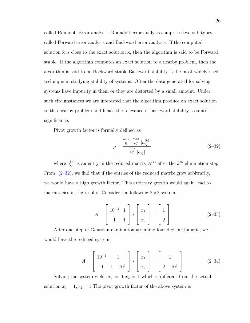
Pivot growth factor is formally defined as
ρ =
max
kmax
ij |a(k)ij |
max
ij |aij|(2–32)
where a(k)ij is an entry in the reduced matrix A(k) after the kth elimination step.
From (2–32), we find that if the entries of the reduced matrix grow arbitrarily,
we would have a high growth factor. This arbitrary growth would again lead to
inaccuracies in the results. Consider the following 2 ∗ 2 system.
A =
10−4 1
1 1
∗
x1
x2
=
1
2
(2–33)
After one step of Gaussian elimination assuming four digit arithmetic, we
would have the reduced system
A =
10−4 1
0 1− 104
∗
x1
x2
=
1
2− 104
(2–34)
Solving the system yields x1 = 0, x2 = 1 which is different from the actual
solution x1 = 1, x2 = 1.The pivot growth factor of the above system is

27
ρ = max(1,104)1
= 104
Thus a large pivot growth clearly indicates the inaccuracy in the result. Partial
pivoting generally avoids large growth factors. In the above example, if we had
applying partial pivoting, we would have got the correct results. But this is not
assured and there are cases where partial pivoting might not result in an acceptable
growth factor. This necessitates the estimation of the growth factor as a diagnostic
tool to detect cases where Gaussian elimination could be unstable.
Pivot growth factor is calculated usually in terms of its reciprocal, to avoid
numerical overflow problems when the value is very large. (2–32) is a harder to
compute equation since it involves calculating the maximum of reduced matrix
after every step of elimination. The other definitions of reciprocal growth factor
that are easy to compute are as follows:
1
ρ=min
j(max
i |aij|)(max
i |uij|)(2–35)
1
ρ=
(max
ij |aij|)(max
ij |uij|)(2–36)
Equation (2–35) is the definition implemented in KLU and it is a column
scaling invariant. It helps unmask a large pivot growth that could be totally
masked because of column scaling.
2.12 Condition Number
Growth factor is a key estimate in determining the stability of the algorithm.
Condition number is a key estimate in determining the amenability or conditioning
of a given problem. It is not guaranteed that a highly stable algorithm can yield
accurate results for all problems it can solve. The conditioning of the problem has
a dominant effect on the accuracy of the solution.
Note that while stability deals with the algorithm, conditioning deals with
the problem itself. In practical applications like circuit simulation, the data of
28
a problem come from experimental observations. Typically such data have a
factor of error or impurities or noise associated with them. Roundoff errors and
discretization errors also contribute to impurities in the data. Conditioning of a
problem deals with determining how the solution of the problem changes in the
presence of impurities.
The preceding discussion shows that one often deals with solving problems
not with the original data but that with perturbed data. The analysis of effect
of perturbation of the problem on the solution is called Perturbation analysis. It
helps in determining whether a given problem produces a little or huge variation
in solution when perturbed. Let us see what we mean by well or ill conditioned
problems.
A problem is said to be ill conditioned if a small relative error in data leads
to a large relative error in solution irrespective of the algorithm employed. A
problem is said to be well conditioned if a small relative error in data does not
lead to a large relative error in solution.
Accuracy of the computed solution is of primary importance in numerical
analysis. Stability of the algorithm and the Conditioning of the given problem are
the two factors that directly determine accuracy.A highly stable algorithm well
armored with scaling, partial pivoting and other concepts cannot be guaranteed to
yield an accurate solution to an ill-conditioned problem.
A backward stable algorithm applied to a well-conditioned problem should
yield a solution close to the exact solution. This follows from the definitions of
backward stability and well-conditioning, where backward stability assures exact
solution to a nearby problem and well-conditioned problem assures that the
computed solution to perturbed data is relatively close to the exact solution of the
actual problem.

29
Mathematically, let X be some problem. Let X(d) be the solution to the
problem for some input d. Let δd denote a small perturbation in the input d. Now
if the relative error in the solution
|X(d+ δd)−X(d)||X(d)|
exceeds the relative error in the input
|δd||d|
then the problem is ill conditioned and well conditioned otherwise.
Condition number is a measure of the conditioning of the problem. It shows
whether a problem is well or ill conditioned.For the linear system problems of the
form Ax = b, the condition number is defined as
Cond(A) = ‖A‖‖A−1‖ (2–37)
Equation (2–37) is arrived at by theory that deals with perturbations either
in the input matrix A or the right hand side b or both the matrix and right hand
side. Equation (2–37) can be defined with respect to any norm viz. 1, 2 or ∞. The
system Ax = b is said to be ill-conditioned if the condition number from (2–37) is
quite large. Otherwise it is said to be well-conditioned.
A naive way to compute the condition number would be to compute the
inverse of the matrix, compute the norm of the matrix and its inverse and compute
the product. However, computing the inverse is atleast thrice as expensive as
solving the linear system Ax = b and hence should be avoided.
Hager [22] developed a method for estimating the 1-norm of ‖A−1‖ and the
corresponding 1-norm condition number. Hager proposed an optimization approach
for estimating ‖A−1‖1. The 1-norm of a matrix is formally defined as

30
‖A‖1 = max‖Ax‖1
‖x‖1
(2–38)
Hager’s algorithm can be briefly described as follows: For A ∈ Rn∗n, a convex
function is defined as
F (x) = ‖Ax‖1 (2–39)
over the convex set
S = {x ∈ Rn : ‖x‖1 ≤ 1}
Then ‖A‖1 is the global maximum of (2–39).
The algorithm involves computing Ax and ATx or computing matrix-vector
products. When we want to compute ‖A−1‖1, it involves computing A−1x and
(A−1)Tx which is equivalent to solving Ax = b and ATx = b. We can use KLU to
efficiently solve these systems.
Higham [23] presents refinements to Hager’s algorithm and restricts the
number of iterations to five. Higham further presents a simple device and using
the higher of the estimates from this device and Hager’s algorithm to ensure the
esimate is large enough. This device involves solving the linear system Ax = b
where
bi = (−1)i+1(1 +i− 1
n− 1), i = 1, 2, ...n
The final estimate is chosen as the maximum from Hager’s algorithm and
2‖x‖13n
.
KLU’s condition number estimator is based on Higham’s refinement of Hager’s
algorithm.
2.13 Depth First Search
As we discussed earlier, the nonzero pattern of the kth column of L is deter-
mined by the Reachability of the row-indices of kth column of A in the graph of L.
31
The reachability is determined by a depth-first search traversal of the graph of L.
The topological order for elimination of variables when solving the lower triangular
system Lx = b is also determined by the depth-first search traversal. A classical
depth first search algorithm is a recursive one. One of the major problems in a
recursive implementation of depth-first search is Stack overflow. Each process is
allocated a stack space upon execution. When there is a high number of recursive
calls, the stack space is exhausted and the process terminates abruptly. This is a
definite possibility in the context of our depth-first search algorithm when we have
a dense column of a matrix of a very high dimension.
The solution to stack overflow caused by recursion is to replace recursion
by iteration. With an iterative or non-recursive function, the entire depth first
search happens in a single function stack. The iterative solution uses an array
of row indices called pstack. When descending to an adjacent node during the
search, the row index of the next adjacent node is stored in the pstack at the
position(row/column index) corresponding to the current node. When the search
returns to the current node, we know that we next need to descend into the node
stored in the pstack at the position corresponding to the current node. Using this
extra O(n) memory, the iterative version completes the depth first search in a
single function stack.
This is an important improvement from the recursive version since it avoids
the stack overflow problem that would have been a bottleneck when solving high
dimension systems.
2.14 Memory Fragmentation
The data structures for L and U are the ones used to represent sparse matri-
ces. These comprise 3 vectors.
1. Vector of column pointers
2. Vector of row indices

32
3. Vector of numerical values
There are overall, six vectors needed for the two matrices L and U. Of these, the
two vectors of column pointers are of pre-known size namely the size of a block.
The remaining four vectors of row indices and numerical values depend on the fill-
in estimated by AMD. However AMD gives an optimistic estimate of fill-in.Hence
we need to dynamically grow memory for these vectors during the factorization
phase if we determine that the fill-in is higher than estimated. The partial pivoting
strategy can alter the row ordering determined by AMD and hence is another
source of higher fill-in than the estimate from AMD.
Dynamically growing these four vectors suffers from the problem of external
memory fragmentation. In external fragmentation, free memory is scattered in
the memory space. A call for more memory fails because of non-availability of
contiguous free memory space. If the scattered free memory areas were contiguous,
the memory request would have succeeded. In the context of our problem, the
memory request to grow the four vectors could either fail if we run into external
fragmentation or succeed when there is enough free space available.
When we reallocate or grow memory, there are two types of success cases. In
the first case called cheap reallocation, there is enough free memory space abutting
the four vectors. Here the memory occupied by a vector is just extended or its end
boundary is increased. The start boundary remains the same. In the second case
called costly reallocation, there is not enough free memory space abutting a vector.
Hence a fresh memory is allocated in another region for the new size of vector and
the contents are copied from old location. Finally the old location is freed.
With four vectors to grow, there is a failure case because of external fragmen-
tation and a costly success case because of costly reallocation. To reduce the failure
case and avoid the costly success case, we have coalesced the four vectors into a
single vector. This new data structure is byte aligned on double boundary. For

33
every column of L and U, the vector contains the row indices and numerical values
of L , followed by the row indices and numerical values of U. Multiple integer row
indices are stored in a single double location . The actual number of integers that
can be stored in a double location varies with platform and is determined dynam-
ically. The common technique of using integer pointer to point to location aligned
on double boundary, is employed to retrieve or save the row indices.
In addition to this coalesced data structure containing the row indices and
numerical values, two more length vectors of size n are needed to contain the length
of each column of L and U . These length vectors are preallocated once and need
not be grown dynamically.
Some Memory management schemes never do cheap reallocation. In such
schemes, the new data structure serves to reduce external fragmentation only.
2.15 Complex Number Support
KLU supports complex matrices and complex right hand sides. KLU also
supports solving the transpose system ATx = b for real matrices and solving the
conjugate transpose system AHx = b for complex matrices. Initially it relied on the
C99 language support for complex numbers. However the C99 specification is not
supported across operating systems. For example, earlier versions of Sun Solaris do
not support C99. To avoid these compatibility issues, KLU no longer relies on C99
and has its own complex arithmetic implementation.
2.16 Parallelism in KLU
When solving a system Ax = b using KLU, we use BTF pre-ordering to
convert A into a block upper triangular form. We apply AMD on each block and
factorize each block one after the other serially. Alternatively, nested dissection can
be applied to each block. Nested dissection ordering converts a block to a doubly
bordered block diagonal form. A doubly bordered block diagonal form is similar to
a block upper triangular form but has nonzeros on the sub diagonal region. These

34
1
2
4
5
3
A Doubly Bordered Block diagonal Matrix Separator Tree
2 1
4
5
3
Figure 2–6: A doubly bordered block diagonal matrix and its corresponding vertexseparator tree
nonzeros form a horizontal strip resembling a border. Similarly the nonzeros in the
region above the diagonal form a corresponding vertical strip.
The doubly bordered block diagonal form can be thought of as a separator
tree. Factorization of the block then involves a post-order traversal of the separator
tree. The nodes in the separator tree can be factorized in parallel. The factor-
ization of a node would additionally involve computing the schur complement of
its parent and of its ancestors in the tree. Once all the children of a node have
updated its schur complement, the node is ready to be factorized and it inturn
computes the schur complement of its parent and its ancestors. The factorization
and computation of schur complement is done in a post-order traversal fashion and
the process stops at the root.
Parallelism can help in reducing the factorization time. It gains importance in
the context of multi processor systems. Work is being done to enable parallelism in
KLU.

CHAPTER 3CIRCUIT SIMULATION: APPLICATION OF KLU
The KLU algorithm comprises the following steps:
1. Unsymmetric Permutation to block upper triangular form. This consists of
two steps.
(a) unsymmetric permutation to ensure a zero free diagonal using maximum
transversal.
(b) symmetric permutation to block upper triangular form by finding the
strongly connected components of the graph.
2. Symmetric permutation of each block(say A) using AMD on A + AT or an
unsymmetric permutation of each block using COLAMD on AAT . These
permutations are fill-in reducing orderings on each block.
3. Factorization of each scaled block using Gilbert-Peierls’ left looking algorithm
with partial pivoting.
4. Solve the system using block-back substitution and account for the off-
diagonal entries. The solution is re-permuted to bring it back to original
order.
Let us first derive the final system that we need to solve taking into account,
the different permutations, scaling and pivoting. The original system to solve is
Ax = b (3–1)
Let R be the diagonal matrix with the scale factors for each row. Applying scaling,
we have
RAx = Rb (3–2)
35

36
Let P’ and Q’ be the row and column permutation matrices that combine the
permutations for maximum transversal and the block upper triangular form
together. Applying these permutations together, we have
P ′RAQ′Q′Tx = P ′Rb. [Q′Q′T = I, the identity matrix] (3–3)
Let P and Q be row and column permutation matrices that club the P’ and Q’
mentioned above with the symmetric permutation produced by AMD and the
partial pivoting row permutation produced by factorization. Now,
PRAQQTx = PRb
or
(PRAQ)QTx = PRb (3–4)
The matrix (PRAQ) consists of two parts viz. the diagonal blocks that are factor-
ized and the off-diagonal elements that are not factorized.
(PRAQ) = LU + F where LU represents the factors of all the blocks
collectively and F represents the entire off diagonal region. Equation (3–4) now
becomes
(LU + F )QTx = PRb (3–5)
x = Q(LU + F )−1(PRb) (3–6)
Equation (3–6) consists of two steps. A block back-substitution i.e. computing
(LU + F )−1(PRb) followed by applying the column permutation Q.
The block-back substitution in (LU + F )−1(PRb) looks cryptic and can be
better explained as follows: Consider a simple 3 ∗ 3 block system
37
L11U11 F12 F13
0 L22U22 F23
0 0 L33U33
∗
X1
X2
X3
=
B1
B2
B3
(3–7)
The equations corresponding to the above system are:
L11U11 ∗X1 + F12 ∗X2 + F13 ∗X3 = B1 (3–8)
L22U22 ∗X2 + F23 ∗X3 = B2 (3–9)
L33U33 ∗X3 = B3 (3–10)
In block back substitution, we first solve (3–10) for X3, and then eliminate X3
from (3–9) and (3–8) using the off-diagonal entries.
Next, we solve (3–9) for X2 and eliminate X2 from (3–8).
Finally we solve (3–8) for X1
3.1 Characteristics of Circuit Matrices
Circuit matrices exhibit certain unique characteristics that makes KLU more
relevant to them. They are very sparse. Because of their high sparsity, BLAS
kernels are not applicable. Circuit matrices often have a few dense rows/columns
that originate from voltage or current sources. These dense rows/columns are
effectively removed by BTF permutation.
Circuit matrices are asymmetric, but the nonzero pattern is roughly symmet-
ric. They are easily permutable to block upper triangular form. Besides, they have
zero-free or nearly zero-free diagonal. Another peculiar feature of circuit matrices is
that the nonzero pattern of each block after permutation to block upper triangular
form, is more symmetric than the original matrix. Typical ordering strategies
applied to the original matrix cause high fill-in whereas when applied to the blocks,
leads to less fill-in.

38
The efficiency of the permutation to block upper triangular form shows in the
fact the entire sub-diagonal region in the matrix has zero work and the off-diagonal
elements do not cause any fill-in since they are not factorized.
3.2 Linear Systems in Circuit Simulation
The linear systems in circuit simulation process originate from solving large
systems of non linear equations using Newton’s method and integrating large stiff
systems of ordinary differential equations. These linear systems consist of the
coefficients matrix A, the unknowns vector x and the right hand side b.
During the course of simulation, the matrix A retains the same nonzero
pattern(structurally unchanged) and only undergoes changes in numerical val-
ues. Thus the initial analysis phase (permutation to ensure zero-free diagonal,
block triangular form and minimum degree ordering on blocks) and factorization
phase(that involves symbolic analysis, partial pivoting and symmetric pruning) can
be restricted to the initial system alone.
Subsequent systems A′x = b where only the numerical values of A′ are different
from A, can be solved using a mechanism called refactorization. Refactorization
simply means to use the same row and column permutations (comprising entire
analysis phase and partial pivoting) computed for the initial system, for solving the
subsequent systems that have changes only in numerical values. Refactorization
substantially reduces run time since the analysis time and factorization time spent
on symbolic analysis, partial pivoting, pruning are avoided. The nonzero pattern
of the factors L and U are the same as for the initial system. Only Numerical
factorization using the pre-computed nonzero pattern and partial pivoting order, is
required.
The solve step follows the factorization/refactorization step. KLU accomodates
solving multiple right hand sides in a single solve step. Upto four right hand sides
can be solved in a single step.

39
3.3 Performance Benchmarks
During my internship at a circuit simulation company, I did performance
benchmarking of KLU vs SuperLU in the simulation environment. The perfor-
mance benchmarks were run on a representative set of examples. The results
of these benchmarks are tabulated as follows. (the size of the matrix created in
simulation is shown in parenthesis).
Table 3–1: Comparison between KLU and SuperLU on overall time and fill-in
Overall time Nonzeros(L+U)Netlist KLU SuperLU Speedup KLU SuperLUProblem1 (301) 1.67 1.24 0.74 1808 1968Problem2 (1879) 734.96 688.52 0.94 13594 13770Problem3 (2076) 56.46 53.38 0.95 16403 16551Problem4 (7598) 89.63 81.85 0.91 52056 54997Problem5 (745) 18.13 16.84 0.93 4156 4231Problem6 (1041) 1336.50 1317.30 0.99 13198 13995Problem7 (33) 0.40 0.32 0.80 157 176Problem8 (10) 4.46 1.570 0.35 40 41Problem9 (180) 222.26 202.29 0.91 1845 1922Problem10(6833) 6222.20 6410.40 1.03 56322 58651Problem11 (1960) 181.78 179.50 0.99 13527 13963Problem12 (200004) 6.25 8.47 1.35 500011 600011Problem13 (20004) 0.47 0.57 1.22 50011 60011Problem14 (40004) 0.97 1.31 1.35 100011 120011Problem15 (100000) 1.76 2.08 1.18 299998 499932Problem16 (7602) 217.80 255.88 1.17 156311 184362Problem17(10922) 671.10 770.58 1.15 267237 299937Problem18 (14842) 1017.00 1238.10 1.22 326811 425661Problem19 (19362) 1099.00 1284.40 1.17 550409 581277Problem20 (24482) 3029.00 3116.90 1.03 684139 788047Problem21 (30202) 2904.00 3507.40 1.21 933131 1049463
The circuits Problem16–Problem21 are TFT LCD arrays similar to memory
circuits. These examples were run atleast twice with each algorithm employed viz.
KLU or SuperLU to get consistent results. The results are tabulated in tables 3–1,
3–2 and 3–3. The ”overall time” in table 3–1 comprises of analysis, factorization
and solve time.

40
Table 3–2: Comparison between KLU and SuperLU on factor time and solve time
Factor time Factor Solve time Solveper iteration speedup per iteration speedup
Netlist KLU SuperLU KLU SuperLUProblem1 (301) 0.000067 0.000084 1.26 0.000020 0.000019 0.92Problem2 (1879) 0.000409 0.000377 0.92 0.000162 0.000100 0.61Problem3 (2076) 0.000352 0.000317 0.90 0.000122 0.000083 0.68Problem4 (7598) 0.001336 0.001318 0.99 0.000677 0.000326 0.48Problem5 (745) 0.000083 0.000063 0.76 0.000035 0.000022 0.62Problem6 (1041) 0.000321 0.000406 1.26 0.000079 0.000075 0.95Problem7 (33) 0.000004 0.000004 0.96 0.000003 0.000002 0.73Problem8 (10) 0.000001 0.000001 0.89 0.000001 0.000001 0.80Problem9 (180) 0.000036 0.000042 1.16 0.000014 0.000011 0.76Problem10(6833) 0.001556 0.001530 0.98 0.000674 0.000365 0.54Problem11 (1960) 0.000663 0.000753 1.14 0.000136 0.000122 0.90Problem12 (200004) 0.103900 0.345500 3.33 0.030640 0.041220 1.35Problem13 (20004) 0.005672 0.020110 3.55 0.001633 0.002735 1.67Problem14 (40004) 0.014430 0.056080 3.89 0.004806 0.006864 1.43Problem15 (100000) 0.168700 0.283700 1.68 0.018600 0.033610 1.81Problem16 (7602) 0.009996 0.017620 1.76 0.001654 0.001439 0.87Problem17(10922) 0.018380 0.030010 1.63 0.002542 0.001783 0.70Problem18 (14842) 0.024020 0.046130 1.92 0.003187 0.002492 0.78Problem19 (19362) 0.054730 0.080280 1.47 0.005321 0.003620 0.68Problem20 (24482) 0.121400 0.122600 1.01 0.006009 0.004705 0.78Problem21 (30202) 0.124000 0.188700 1.52 0.009268 0.006778 0.73
41
3.4 Analyses and Findings
The following are my inferences based on the results: Most of the matrices in
these experiments are small matrices of the order of a few thousands.
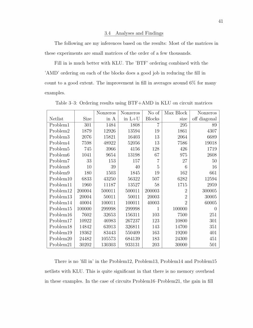
Fill in is much better with KLU. The ’BTF’ ordering combined with the
’AMD’ ordering on each of the blocks does a good job in reducing the fill in
count to a good extent. The improvement in fill in averages around 6% for many
examples.
Table 3–3: Ordering results using BTF+AMD in KLU on circuit matrices
Nonzeros Nonzeros No of Max Block NonzerosNetlist Size in A in L+U Blocks size off diagonalProblem1 301 1484 1808 7 295 89Problem2 1879 12926 13594 19 1861 4307Problem3 2076 15821 16403 13 2064 6689Problem4 7598 48922 52056 13 7586 19018Problem5 745 3966 4156 128 426 1719Problem6 1041 9654 13198 67 975 2608Problem7 33 153 157 7 27 50Problem8 10 39 40 5 6 16Problem9 180 1503 1845 19 162 661Problem10 6833 43250 56322 507 6282 12594Problem11 1960 11187 13527 58 1715 2959Problem12 200004 500011 500011 200003 2 300005Problem13 20004 50011 50011 20003 2 30005Problem14 40004 100011 100011 40003 2 60005Problem15 100000 299998 299998 1 100000 0Problem16 7602 32653 156311 103 7500 251Problem17 10922 46983 267237 123 10800 301Problem18 14842 63913 326811 143 14700 351Problem19 19362 83443 550409 163 19200 401Problem20 24482 105573 684139 183 24300 451Problem21 30202 130303 933131 203 30000 501
There is no ’fill in’ in the Problem12, Problem13, Problem14 and Problem15
netlists with KLU. This is quite significant in that there is no memory overhead
in these examples. In the case of circuits Problem16–Problem21, the gain in fill

42
in with KLU ranges from 6% in the Problem19 example to 24% in Problem18
example.
The gain in fill in translates into faster factorization because few nonzeros
imply less work. The factorization time thus is expected to be low. It turns out
to be true in most of the cases (factorization speedup of 1.6x in Problem16–
Problem21 examples and 3x for Problem12–Problem14 examples). For some cases
like Problem2 and Problem10, the factorization time remains same for both KLU
and SuperLU.
Solve phase turns out to be slow in KLU. Probably, the off diagonal nonzero
handling part tends to account for the extra time spent in the solve phase.
One way of reducing the solve overhead in KLU would be solving multiple
RHS at the same time. In a single solve iteration, 4 equations are solved.
On the whole, the overall time speedup is 1.2 for Problem16–Problem21
examples and Problem12–Problem14 examples. For others, the overall time is
almost the same between the two algorithms.
BTF is not able to find out many blocks for most of the matrices and there
happens to be a single large block and the remaining are singletons. But the AMD
ordering does a good job in getting the fill in count reduced. The off-diagonal
nonzero count is not high.
3.5 Alternate Ordering Experiments
Different ordering strategies were employed to analyze the fill in behaviour.
The statistics using different ordering schemes are listed in table 3–4. ’COLAMD’
is not listed in the table. It typically gives poor ordering and causes more fill
in than AMD, MMD and AMD+BTF. AMD alone gives relatively higher fill in
compared to AMD+BTF in most of the matrices. However AMD alone gives mixed
results in comparison with MMD. It matches or outperforms MMD in fill in on
Problem12–Problem14 and Problem16–Problem21 matrices. However it gives
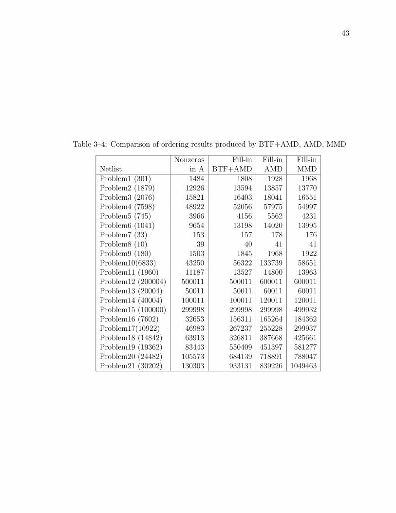
43
Table 3–4: Comparison of ordering results produced by BTF+AMD, AMD, MMD
Nonzeros Fill-in Fill-in Fill-inNetlist in A BTF+AMD AMD MMDProblem1 (301) 1484 1808 1928 1968Problem2 (1879) 12926 13594 13857 13770Problem3 (2076) 15821 16403 18041 16551Problem4 (7598) 48922 52056 57975 54997Problem5 (745) 3966 4156 5562 4231Problem6 (1041) 9654 13198 14020 13995Problem7 (33) 153 157 178 176Problem8 (10) 39 40 41 41Problem9 (180) 1503 1845 1968 1922Problem10(6833) 43250 56322 133739 58651Problem11 (1960) 11187 13527 14800 13963Problem12 (200004) 500011 500011 600011 600011Problem13 (20004) 50011 50011 60011 60011Problem14 (40004) 100011 100011 120011 120011Problem15 (100000) 299998 299998 299998 499932Problem16 (7602) 32653 156311 165264 184362Problem17(10922) 46983 267237 255228 299937Problem18 (14842) 63913 326811 387668 425661Problem19 (19362) 83443 550409 451397 581277Problem20 (24482) 105573 684139 718891 788047Problem21 (30202) 130303 933131 839226 1049463
44
poor fill in for rest of the circuits when compared with MMD. AMD alone beats
AMD+BTF in fill-in for some of the examples viz. Problem17, Problem19 and
Problem21. Overall, to sum it up, BTF+AMD is the best ordering strategy to use.
3.6 Experiments with UF Sparse Matrix Collection
There are a number of circuit matrices in the UF sparse matrix collection.
Different experiments were done with these matrices as well on different parameters
like
1. ordering quality with different ordering schemes in KLU
2. timing of different phases of KLU
3. ordering quality among KLU, UMFPACK and Gilbert-Peierls’ Algorithm
4. performance comparison between KLU and UMFPACK.
UMFPACK is a unsymmetric multifrontal sparse solver and uses an unsymmetric
COLAMD ordering or an AMD ordering, automatically selecting which method
to use based on the matrix characteristics. Gilbert-Peierls’ algorithm is available
in MATLAB as an LU factorization scheme. These experiments were done on a
Mandrake 10.0 linux OS, Intel Pentium M Processor with clock frequency of 1400
MHz and RAM 768 kB.
3.6.1 Different Ordering Schemes in KLU
There are six different ordering schemes possible in KLU. The three fill
reducing schemes are AMD, COLAMD and User Specified Ordering. These
three fill reducing orderings can be combined with a BTF preordering or no
preordering.Hence six different schemes. However in this experiment user specified
ordering is not considered. That leaves us with four different schemes.The table
3–5 lists the fill (number of nonzeros in L+U plus the number of off-diagonal
elements) for each of these ordering schemes.
From table 3–5, we find that BTF+AMD gives consistently better fill-in
across different circuit matrices. However there are observable aberrations. For

45
example, with the circuit Bomhof/circuit 2, AMD and COLAMD give better fill-in
than BTF+AMD. These results determine again that BTF+AMD is the best
ordering scheme to use for circuit matrices.
3.6.2 Timing Different Phases in KLU
These experiments show the time spent in different phases of the algorithm.
BTF pre-ordering followed by a AMD fill-reducing ordering is employed. As
mentioned earlier, there are four different phases.
1. Analysis phase: This comprises the pre-ordering and fill reducing ordering.
2. Factor phase: This comprises the factorization part of the algorithm. It
includes the symbolic analysis phase, partial pivoting, symmetric pruning
steps.
3. Refactor phase: This comprises the part where we do a factorization using the
already pre-computed partial pivoting permutation and the nonzero pattern
of the L and U matrices. There is no symbolic analysis, partial pivoting and
symmetric pruning in refactor phase.
4. Solve phase: This comprises the solve phase of the algorithm. Solving a single
right hand side was experimented.
When given a set of matrices with the same nonzero pattern, the analysis
and factor phases are done only once. The refactor phase is then repeated for the
remaining matrices. Solve phase is repeated as many times as there are systems
to solve. Table 3–6 consists of the timing results. Analysis phase consumes most
of the time spent in the algorithm. Refactor time is typically 3 or 4 times smaller
than factor time and 8 times smaller than analysis time plus factor time put
together. Solve phase consumes the least fraction of time spent.
3.6.3 Ordering Quality among KLU, UMFPACK and Gilbert-Peierls
The table 3–7 compares the ordering quality among KLU using BTF+AMD,
UMFPACK using COLAMD or AMD and Gilbert-Peierls’ using AMD. We can

46
Table 3–5: Fill-in with four different schemes in KLU
Nonzeros BTF + BTF +Matrix in A AMD COLAMD AMD COLAMDSandia/adder dcop 01 (1813) 11156 13525 13895 18848 21799Sandia/adder trans 01 (1814) 14579 20769 36711 24365 119519Sandia/fpga dcop 01 (1220) 5892 7891 8118 8869 12016Sandia/fpga trans 01 (1220) 7382 10152 12776 10669 21051Sandia/init adder1 (1813) 11156 13525 13895 18848 21799Sandia/mult dcop 01 (25187) 193276 226673 228301 2176328 1460322Sandia/oscil dcop 01 (430) 1544 2934 3086 3078 3295Sandia/oscil trans 01 (430) 1614 2842 3247 2897 3259Bomhof/circuit 1 (2624) 35823 44879 775363 44815 775720Bomhof/circuit 2 (4510) 21199 40434 89315 36197 36196Bomhof/circuit 3 (12127) 48137 86718 98911 245336 744245Grund/b2 ss (1089) 3895 9994 9212 26971 9334Grund/b dyn (1089) 4144 11806 10597 33057 10544Grund/bayer02 (13935) 63307 889914 245259 1365142 307979Grund/d dyn (87) 230 481 461 619 494Grund/d ss (53) 144 302 292 382 298Grund/meg1 (2904) 58142 232042 184471 1526780 378904Grund/meg4 (5860) 25258 42398 310126 43250 328144Grund/poli (4008) 8188 12200 12208 12238 12453Grund/poli large (15575) 33033 48718 48817 49806 51970Hamm/add20 (2395) 13151 19554 34636 19554 34636Hamm/add32 (4960) 19848 28754 36030 28754 36030Hamm/bcircuit (68902) 375558 1033240 1692668 1033240 1692668Hamm/hcircuit (105676) 513072 731634 2623852 736080 4425310Hamm/memplus (17758) 99147 137030 3282586 137030 3282586Hamm/scircuit (170998) 958936 2481122 6410286 2481832 6427526Rajat/rajat03 (7602) 32653 163913 235111 172666 236938Rajat/rajat04 (1041) 8725 12863 80518 18618 158000Rajat/rajat05 (301) 1250 1926 2053 2101 3131Rajat/rajat11 (135) 665 890 978 944 1129Rajat/rajat12 (1879) 12818 15308 273667 15571 128317Rajat/rajat13 (7598) 48762 58856 90368 64791 5234287Rajat/rajat14 (180) 1475 1994 2249 2105 2345
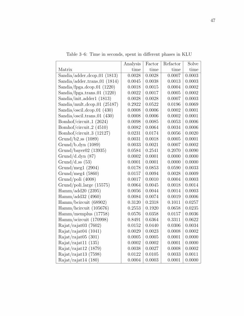
47
Table 3–6: Time in seconds, spent in different phases in KLU
Analysis Factor Refactor SolveMatrix time time time timeSandia/adder dcop 01 (1813) 0.0028 0.0028 0.0007 0.0003Sandia/adder trans 01 (1814) 0.0045 0.0038 0.0013 0.0003Sandia/fpga dcop 01 (1220) 0.0018 0.0015 0.0004 0.0002Sandia/fpga trans 01 (1220) 0.0022 0.0017 0.0005 0.0002Sandia/init adder1 (1813) 0.0028 0.0028 0.0007 0.0003Sandia/mult dcop 01 (25187) 0.2922 0.0522 0.0196 0.0069Sandia/oscil dcop 01 (430) 0.0008 0.0006 0.0002 0.0001Sandia/oscil trans 01 (430) 0.0008 0.0006 0.0002 0.0001Bomhof/circuit 1 (2624) 0.0098 0.0085 0.0053 0.0006Bomhof/circuit 2 (4510) 0.0082 0.0064 0.0034 0.0006Bomhof/circuit 3 (12127) 0.0231 0.0174 0.0056 0.0020Grund/b2 ss (1089) 0.0031 0.0018 0.0005 0.0001Grund/b dyn (1089) 0.0033 0.0021 0.0007 0.0002Grund/bayer02 (13935) 0.0584 0.2541 0.2070 0.0090Grund/d dyn (87) 0.0002 0.0001 0.0000 0.0000Grund/d ss (53) 0.0001 0.0001 0.0000 0.0000Grund/meg1 (2904) 0.0178 0.0853 0.0590 0.0033Grund/meg4 (5860) 0.0157 0.0094 0.0028 0.0009Grund/poli (4008) 0.0017 0.0010 0.0004 0.0003Grund/poli large (15575) 0.0064 0.0045 0.0018 0.0014Hamm/add20 (2395) 0.0056 0.0044 0.0014 0.0003Hamm/add32 (4960) 0.0084 0.0074 0.0019 0.0006Hamm/bcircuit (68902) 0.3120 0.2318 0.1011 0.0257Hamm/hcircuit (105676) 0.2553 0.1920 0.0658 0.0235Hamm/memplus (17758) 0.0576 0.0358 0.0157 0.0036Hamm/scircuit (170998) 0.8491 0.6364 0.3311 0.0622Rajat/rajat03 (7602) 0.0152 0.0440 0.0306 0.0034Rajat/rajat04 (1041) 0.0029 0.0023 0.0008 0.0002Rajat/rajat05 (301) 0.0005 0.0005 0.0001 0.0000Rajat/rajat11 (135) 0.0002 0.0002 0.0001 0.0000Rajat/rajat12 (1879) 0.0038 0.0027 0.0008 0.0002Rajat/rajat13 (7598) 0.0122 0.0105 0.0033 0.0011Rajat/rajat14 (180) 0.0004 0.0003 0.0001 0.0000

48
infer from the results that KLU produces better ordering than UMFPACK and
Gilbert-Peierls’ algorithm. For KLU, the following MATLAB code determines the
fill.
opts = [0.1 1.2 1.2 10 1 0 0 0 ] ;
[x info] = klus(A,b,opts, []) ;
fill = info (31) + info (32) + info(8) ;
For UMFPACK, the snippet is
[L U P Q] = lu(A) ;
fill = nnz(L) + nnz(U) ;
For Gilbert-Peierls’ the code is
Q = amd(A) ;
[L U P] = lu(A(Q,Q), 0.1) ;
fill = nnz(L) + nnz(U) ;
3.6.4 Performance Comparison between KLU and UMFPACK
This experiment compares the total time spent in the analysis, factor and solve
phases by the algorithms. The results are listed in table 3–8. KLU outperforms
UMFPACK in time. For KLU, the following snippet in MATLAB is used:
tic
[x info] = klus(A,b,opts) ;
t1 = toc ;
For UMFPACK, the following code in MATLAB is used to find the total time:
tic
x = A \ b ;
t2 = toc ;

49
Table 3–7: Fill-in among KLU, UMFPACK and Gilbert-Peierls
Matrix nnz KLU UMFPACK Gilbert-PeierlsSandia/adder dcop 01 (1813) 11156 13525 14658 18825Sandia/adder trans 01 (1814) 14579 20769 20769 24365Sandia/fpga dcop 01 (1220) 5892 7891 8106 8869Sandia/fpga trans 01 (1220) 7382 10152 10152 10669Sandia/init adder1 (1813) 11156 13525 14658 18825Sandia/mult dcop 01 (25187) 193276 226673 556746 1300902Sandia/oscil dcop 01 (430) 1544 2934 2852 3198Sandia/oscil trans 01 (430) 1614 2842 3069 2897Bomhof/circuit 1 (2624) 35823 44879 44879 44815Bomhof/circuit 2 (4510) 21199 40434 35107 38618Bomhof/circuit 3 (12127) 48137 86718 84117 245323Grund/b2 ss (1089) 3895 9994 8309 22444Grund/b dyn (1089) 4144 11806 9642 41092Grund/bayer02 (13935) 63307 889914 259329 973093Grund/d dyn (87) 230 481 442 523Grund/d ss (53) 144 302 268 395Grund/meg1 (2904) 58142 232042 151740 1212904Grund/meg4 (5860) 25258 42398 42398 43250Grund/poli (4008) 8188 12200 12200 12239Grund/poli large (15575) 33033 48718 48745 49803Hamm/add20 (2395) 13151 19554 19554 19554Hamm/add32 (4960) 19848 28754 28754 28754Hamm/bcircuit (68902) 375558 1033240 1033240 1033240Hamm/hcircuit (105676) 513072 731634 730906 736080Hamm/memplus (17758) 99147 137030 137030 137030Hamm/scircuit (170998) 958936 2481122 2481122 2481832Rajat/rajat03 (7602) 32653 163913 163913 172666Rajat/rajat04 (1041) 8725 12863 12860 18613Rajat/rajat05 (301) 1250 1926 1944 2101Rajat/rajat11 (135) 665 890 890 944Rajat/rajat12 (1879) 12818 15308 15308 15571Rajat/rajat13 (7598) 48762 58856 58856 64791Rajat/rajat14 (180) 1475 1994 1994 2105

50
Table 3–8: Performance comparison between KLU and UMFPACK
Matrix KLU UMFPACKSandia/adder dcop 01 (1813) 0.0116 0.0344Sandia/adder trans 01 (1814) 0.0112 0.0401Sandia/fpga dcop 01 (1220) 0.0050 0.0257Sandia/fpga trans 01 (1220) 0.0054 0.0203Sandia/init adder1 (1813) 0.0109 0.0323Sandia/mult dcop 01 (25187) 1.2383 1.1615Sandia/oscil dcop 01 (430) 0.0022 0.0070Sandia/oscil trans 01 (430) 0.0019 0.0074Bomhof/circuit 1 (2624) 0.0232 0.1223Bomhof/circuit 2 (4510) 0.0201 0.0522Bomhof/circuit 3 (12127) 0.0579 0.1713Grund/b2 ss (1089) 0.0066 0.0168Grund/b dyn (1089) 0.0072 0.0175Grund/bayer02 (13935) 0.6089 0.3565Grund/d dyn (87) 0.0005 0.0014Grund/d ss (53) 0.0003 0.0010Grund/meg1 (2904) 0.1326 0.1018Grund/meg4 (5860) 0.0571 0.1111Grund/poli (4008) 0.0050 0.0121Grund/poli large (15575) 0.0208 0.0497Hamm/add20 (2395) 0.0123 0.0506Hamm/add32 (4960) 0.0201 0.0738Hamm/bcircuit (68902) 0.7213 1.8823Hamm/hcircuit (105676) 0.7313 2.7764Hamm/memplus (17758) 0.1232 0.8140Hamm/scircuit (170998) 1.9812 7.3448Rajat/rajat03 (7602) 0.0793 0.1883Rajat/rajat04 (1041) 0.0068 0.0284Rajat/rajat05 (301) 0.0014 0.0046Rajat/rajat11 (135) 0.0007 0.0023Rajat/rajat12 (1879) 0.0087 0.0355Rajat/rajat13 (7598) 0.0330 0.1229Rajat/rajat14 (180) 0.0010 0.0032
CHAPTER 4USER GUIDE FOR KLU
4.1 The Primary KLU Structures
4.1.1 klu common
This is a control structure that contains both input control parameters for
KLU as well as output statistics computed by the algorithm. It is a mandatory
parameter for all the KLU routines. Its contents are listed as follows:
• tol
Type: double
Input parameter for pivot tolerance for diagonal preference.Default value is
0.001
• growth
Type: double
Input parameter for reallocation growth size of LU factors. Default value is
1.2
• initmem amd
Type: double
Input parameter for initial memory size with AMD.
Initial memory size = initmem amd * nnz(L) + n. Default value is 1.2
• initmem
Type: double
Input parameter for initial memory size with COLAMD.
Initial memory size = initmem * nnz(A) + n. Default value is 10
• btf
Type: int
51

52
Input parameter to use BTF pre-ordering, or not. Default value is 1 (to use
BTF)
• ordering
Type: int
Input parameter to specify which fill reducing ordering to use.
0= AMD,1= COLAMD, 2= user P and Q. Default is 0.
• scale
Type: int
Input parameter to specify which scaling strategy to use. 0= none, 1= sum,
2= max. Default is 0
• singular proc
Type: int
Input parameter to specify whether to stop on singularity or continue.
0= stop, 1= continue. Default is 0.
• status
Type: int
Output parameter that indicates the result of the KLU function call. Values
are KLU OK(0) if OK and < 0 if error. Error values are KLU SINGULAR
(-1), KLU OUT OF MEMORY (-2), KLU INVALID (-3)
• nrealloc
Type: int
Output parameter.Contains number of reallocations of L and U
• singular col
Type: int
Output parameter.Contains the column no of singular column if any
• noffdiag
Type: int

53
Output parameter.Contains the number of off-diagonal pivots chosen
4.1.2 klu symbolic
This structure encapsulates the information related to the analysis phase. The
members of the structure are listed as follows:
• symmetry
Type: double
Contains the symmetry of largest block
• est flops
Type: double
Contains the estimated factorization flop count
• lnz
Type: double
Contains the estimated nonzeros in L including diagonals
• unz
Type: double
Contains the estimated nonzeros in U including diagonals
• Lnz
Type: double *
Array of size n, but only Lnz [0..nblocks-1] is used. Contains the estimated
number of nonzeros in each block
• n
Type: int
Contains the size of input matrix A where A is n-by-n
• nz
Type: int
Contains the number of entries in input matrix
• P

54
Type: int *
Array of size n. Contains the row permutation from ordering
• Q
Type: int *
Array of size n. Contains the column permutation from ordering
• R
Type: int *
Array of size n+1, but only R [0..nblocks] is used. Contains the start and end
column/row index for each block. Block k goes from R[k] to R[k+1] - 1
• nzoff
Type: int
Contains the number of nonzeros in off-diagonal blocks
• nblocks Type: int
Contains the number of blocks
• maxblock
Type: int
Contains the size of largest block
• ordering
Type: int
Contains the ordering used (0 = AMD, 1 = COLAMD, 2 = GIVEN)
• do btf
Type: int
Indicates whether or not BTF preordering was requested
The members symmetry, est flops, lnz, unz, Lnz are computed only when AMD is
used. The remaining members are computed for all orderings.

55
4.1.3 klu numeric
This structure encapsulates information related to the factor phase. It contains
the LU factors of each block, pivot row permutation, and the entries in the off-
diagonal blocks among others. Its contents are listed as follows:
• umin
Type: double
Contains the minimum absolute diagonal entry in U
• umax
Type: double
Contains the maximum absolute diagonal entry in U
• nblocks
Type: int
Contains the number of blocks
• lnz
Type: int
Contains actual number of nonzeros in L excluding diagonals
• unz
Type: int
Contains actual number of nonzeros in U excluding diagonals
• Pnum
Type: int *
Array of size n.Contains the final pivot permutation
• Pinv
Type: int *
Array of size n.Contains the inverse of final pivot permutation
• Lbip
Type: int **

56
Array of size nblocks. Each element is an array of size block size + 1. Each
element contains the column pointers for L factor of the corresponding block
• Ubip
Type: int **
Array of size nblocks. Each element is an array of size block size + 1. Each
element contains the column pointers for U factor of the corresponding block
• Lblen
Type: int **
Array of size nblocks. Each element is an array of size block size. Each
element contains the column lengths for L factor of the corresponding block
• Ublen
Type: int **
Array of size nblocks. Each element is an array of size block size. Each
element contains the column lengths for U factor of the corresponding block
• LUbx
Type: void **
Array of size nblocks. Each element is an array containing the row indices
and numerical values of LU factors of the corresponding block. The diagonals
of LU factors are not stored here
• Udiag
Type: void **
Array of size nblocks.Each element is an array of size block size. Each
element contains the diagonal values of U factor of the corresponding block
• Singleton
Type: void *
Array of size nblocks.Contains the singleton values
• Rs
57
Type: double *
Array of size n. Contains the row scaling factors
• scale
Type: int
Indicates the scaling strategy used.
(0 = none, 1 = sum, 2 = max)
• Work
Type: void *
Permanent workspace used for factorization and solve. It is of size
MAX (4n numerical values, n numerical values + 6*maxblock int’s)
• worksize
Type: size t
Contains the size (in bytes) of Work allocated above
• Xwork
Type: void *
This is an alias into Numeric-¿Work
• Iwork
Type: int *
An integer alias into Xwork + n
• Offp
Type: int *
Array of size n+1. Contains the column pointers for off-diagonal elements.
• Offi
Type: int *
Array of size number of off-diagonal entries. Contains the row indices of
off-diagonal elements
• Offx

58
Type: void *
Array of size number of off-diagonal entries. Contains the numerical values of
off-diagonal elements
4.2 KLU Routines
The user callable KLU routines in the C language are explained in this section.
The following guidelines are applicable to all routines except when explicitly stated
otherwise in the description of a routine.
1. : All the arguments are required except when explicitly stated as optional. If
optional, a user can pass NULL for the corresponding argument.
2. : The control input/output argument ”Common” of type ”klu common *” is
a required argument for all routines.
3. : All arguments other than the above mentioned control argument ”Com-
mon”, are input arguments and are not modified.
4.2.1 klu analyze
klu_symbolic *klu_analyze
(
int n,
int Ap [ ],
int Ai [ ],
klu_common *Common
) ;
This routine orders the matrix using BTF if specified and the fill reducing
ordering specified.
• Returns a pointer to klu symbolic structure that contains the ordering
information.
• All arguments are required
– n: Size of the input matrix A where A is n*n.
– Ap: Array of column pointers for the input matrix. Size n+1.
59
– Ai: Array of row indices. Size number of nonzeros in A.
– Common: The control input/output structure.
4.2.2 klu analyze given
klu_symbolic *klu_analyze_given
(
int n,
int Ap [ ],
int Ai [ ],
int Puser [ ],
int Quser [ ],
klu_common *Common
) ;
This routine orders the matrix using BTF if specified and the given Puser and
QUser as fill reducing ordering. If Puser and Quser are NULL, then the natural
ordering is used.
• Returns a pointer to klu symbolic structure that contains the ordering
information.
• Arguments
– n: Size of the input matrix A where A is n*n. Required.
– Ap: Array of column pointers for the input matrix. Size n+1. Required.
– Ai: Array of row indices. Size number of nonzeros in A. Required.
– Puser: Optional row permutation to use.
– Quser: Optional column permutation to use.
– Common: The control input/output structure.
4.2.3 klu *factor
klu_numeric *Numeric klu_factor
(
int Ap [ ],
int Ai [ ],

60
double Ax [ ],
klu_symbolic *Symbolic,
klu_common *Common
) ;
This routine factors a real matrix. There is a complex version of this routine
klu z factor that factors a complex matrix and has same function declaration as
klu factor. Both use the results of a call to klu analyze.
• Returns a pointer to klu numeric if successful. NULL otherwise.
• All the arguments are required.
– Ap: Array of column pointers for the input matrix. Size n+1.
– Ai: Array of row indices. Size number of nonzeros in A.
– Ax: Array of numerical values. Size number of nonzeros in A. In the
complex case, the array should consist of real and imaginary parts of
each numerical value as adjacent pairs.
– Symbolic: The structure that contains the results from a call to
klu analyze.
– Common: The control input/output structure. The status field in
Common is set to indicate if the routine was successful or not.
4.2.4 klu *solve
void klu_solve
(
klu_symbolic *Symbolic,
klu_numeric *Numeric,
int ldim,
int nrhs,
double B [ ],
klu_common *Common
) ;
61
This routine solves a real system. There is a complex version of this routine
klu z solve, that solves a complex system and has the same function declaration as
klu solve. Both use the results of a call to klu analyze and klu *factor.
• Return type is void. The rhs vector B is overwritten with the solution.
• All Arguments are required.
– Symbolic: The structure that contains the results from a call to
klu analyze.
– Numeric: The structure that contains the results from a call to
klu *factor.
– ldim: The leading dimension of the right hand side B.
– nrhs: The number of right hand sides being solved.
– B: The right hand side. It is a vector of length ldim * nrhs. It can
be real or complex depending on whether a real or complex system
is being solved. If complex, the real and imaginary parts of the rhs
numerical value must be stored as adjacent pairs. It is overwritten with
the solution.
– Common: The control input/output structure.
4.2.5 klu *tsolve
void klu_tsolve
(
klu_symbolic *Symbolic,
klu_numeric *Numeric,
int ldim,
int nrhs,
int conj_solve,
double B [ ],
klu_common *Common
) ;
62
This routine is similar to klu solve except that it solves a transpose system
A′x = b. This routine solves a real system. Again there is a complex version of
this routine klu z tsolve for solving complex systems and has the same function
declaration as klu tsolve. It also offers to do a conjugate transpose solve for the
complex system AHx = b.
• Return type is void. The rhs vector B is overwritten with the solution.
• All arguments are required. The descriptions for all arguments except
conj solve are same as those for klu *solve. The argument conj solve is
relevant only for complex case. It takes two values 1 = CONJUGATE
TRANSPOSE SOLVE, 0 = TRANSPOSE SOLVE.
4.2.6 klu *refactor
void klu_refactor
(
int Ap [ ],
int Ai [ ],
double Ax [ ],
klu_symbolic *Symbolic,
klu_numeric *Numeric,
klu_common *Common
) ;
This routine does a refactor of the matrix using the previously computed
ordering information in Symbolic and the nonzero pattern of the LU factors in
Numeric objects. It assumes same partial pivoting order computed in Numeric. It
changes only the numerical values of the LU factors stored in Numeric object. It
has a complex version klu z refactor with the same function prototype to handle
complex cases.
• Return type is void. The numerical values of LU factors in Numeric parame-
ter are updated.
• All arguments are required.
63
– Ap: Array of column pointers for the input matrix. Size n+1.
– Ai: Array of row indices. Size number of nonzeros in A.
– Ax: Array of numerical values. Size number of nonzeros in A. In the
complex case, the array should consist of real and imaginary parts of
each numerical value as adjacent pairs.
– Symbolic: The structure that contains the results from a call to
klu analyze.
– Numeric: Input/output argument. The structure contains the results
from a call to klu *factor. The numerical values of LU factors are
overwritten with the ones for the current matrix being factorized.
– Common: The control input/output structure. The status field in
Common is set to indicate if the routine was successful or not.
4.2.7 klu defaults
void klu_defaults
(
klu_common *Common
) ;
This routine sets the default values for the control input parameters of
the klu common object. The default values are listed in the description of the
klu common structure. A call to this routine is required unless the user sets the
control input parameters explicitly.
• Return type is void.
• The argument Common is required. The control input parameters in Com-
mon are set to default values.
4.2.8 klu *rec pivot growth
double klu_rec_pivot_growth
(
int Ap [ ],
64
int Ai [ ],
double Ax [ ],
klu_symbolic *Symbolic,
klu_numeric *Numeric,
klu_common *Common
) ;
This routine computes the reciprocal pivot growth of the factorization algo-
rithm. The complex version of this routine klu z rec pivot growth handles complex
matrices and has the same function declaration.
• The pivot growth estimate is returned.
• All arguments are required.
– Ap: Array of column pointers for the input matrix. Size n+1.
– Ai: Array of row indices. Size number of nonzeros in A.
– Ax: Array of numerical values. Size number of nonzeros in A. In the
complex case, the array should consist of real and imaginary parts of
each numerical value as adjacent pairs.
– Symbolic: The structure that contains the results from a call to
klu analyze.
– Numeric: The structure that contains the results from a call to
klu *factor.
– Common: The control input/output structure. The status field in
Common is set to indicate if the routine was successful or not.
4.2.9 klu *estimate cond number
double klu_estimate_cond_number
(
int Ap [ ],
double Ax [ ],
klu_symbolic *Symbolic,
klu_numeric *Numeric,

65
klu_common *Common
);
This routine computes the condition number estimate of the input matrix. As
before, the complex version of this routine klu z estimate cond number has the
same function declaration and handles complex matrices.
• The condition number estimate is returned.
• All arguments are required.
– Ap: Array of column pointers for the input matrix. Size n+1.
– Ax: Array of numerical values. Size number of nonzeros in A. In the
complex case, the array should consist of real and imaginary parts of
each numerical value as adjacent pairs.
– Symbolic: The structure that contains the results from a call to
klu analyze.
– Numeric: The structure that contains the results from a call to
klu *factor.
– Common: The control input/output structure. The status field in
Common is set to indicate if the routine was successful or not.
4.2.10 klu free symbolic
void klu_free_symbolic
(
klu_symbolic **Symbolic,
klu_common *Common
) ;
This routine deallocates or frees the contents of the klu symbolic object. The
Symbolic parameter must be a valid object computed by a call to klu analyze or
klu analyze given.
• Return type is void.
• All arguments are required.

66
– Symbolic: Input/Output argument. Must be a valid object computed
by a call to klu analyze or klu analyze given. If NULL, the routine just
returns.
– Common: The control input/output structure.
4.2.11 klu free numeric
void klu_free_numeric
(
klu_numeric **Numeric,
klu_common *Common
) ;
This routine frees the klu numeric object computed by a call to klu factor
or klu z factor routines. It resets the pointer to klu numeric to NULL. There is a
complex version of this routine called klu z free numeric with the same function
declaration to handle the complex case.
• Return type is void.
• All arguments are required.
– Numeric. Input/Output argument. The contents of the klu numeric
object are freed. The pointer to klu numeric object is set to NULL.
– Common: The control input/output structure.

REFERENCES
[1] C. L. Lawson, R. J. Hanson, D. Kincaid, and F. T. Krogh, Basic linearalgebra subprograms for FORTRAN usage, ACM Trans. Math. Soft., 5:308–323, 1979.
[2] J. J. Dongarra, J. Du Croz, S. Hammarling, and R. J. Hanson, An extendedset of FORTRAN basic linear algebra subprograms, ACM Trans. Math. Soft.,14: 1–17, 1988.
[3] J. J. Dongarra, J. Du Croz, S. Hammarling, and R. J. Hanson, Algorithm656: An extended set of FORTRAN basic linear algebra subprograms, ACMTrans. Math. Soft., 14: 18–32, 1988.
[4] J. J. Dongarra, J. Du Croz, I. S. Duff, and S. Hammarling, A set of level 3basic linear algebra subprograms, ACM Trans. Math. Soft., 16: 1–17, 1990.
[5] J. J. Dongarra, J. Du Croz, I. S. Duff, and S. Hammarling, Algorithm 679: Aset of level 3 basic linear algebra subprograms, ACM Trans. Math. Soft., 16:18–28, 1990.
[6] James W. Demmel, Stanley C. Eisenstat, John R. Gilbert, Xiaoye S. Li andJoseph W. H. Liu, A supernodal approach to sparse partial pivoting, SIAM J.Matrix Analysis and Applications, 20(3): 720–755, 1999.
[7] Timothy A. Davis, I.S.Duff, An unsymmetric-pattern multifrontal methodfor sparse LU factorization, SIAM J. Matrix Analysis and Applic., 18(1):140–158, 1997.
[8] Timothy A. Davis, Algorithm 832: UMFPACK, an unsymmetric-patternmultifrontal method with a column pre-ordering strategy, ACM Trans. Math.Software, 30(2): 196–199, 2004.
[9] John R.Gilbert and Tim Peierls, Sparse partial pivoting in time proportionalto arithmetic operations, SIAM J. Sci. Stat. Comput., 9(5): 862–873, 1988.
[10] A. George and E. Ng, An implementation of Gaussian elimination withpartial pivoting for sparse systems. SIAM J. Sci. Statist. Comput., 6(2):390–409, 1985.
[11] Iain S. Duff, On algorithms for obtaining a maximum transversal, ACMTransactions on Mathematical Software, 7(3): 315–330, 1981.
67

68
[12] Iain S. Duff, Algorithm 575 permutations for a zero-free diagonal, ACMTransactions on Mathematical Software, 7(3): 387–390, 1981.
[13] Iain S. Duff and John K. Reid, Algorithm 529: permutations to blocktriangular form, ACM Trans. on Mathematical Software, 4(2): 189–192, 1978.
[14] Iain S. Duff and John K. Reid, An implementation of Tarjan’s algorithmfor the block triangular form of a matrix, ACM Trans. on MathematicalSoftware, 4(2): 137–147, 1978.
[15] R.E. Tarjan, Depth first search and linear graph algorithms, SIAM J.Computing., 1: 146–160, 1972.
[16] Thomas H. Cormen, Charles E. Leiserson, Ronald L. Rivest, Clifford Stein,Introduction to Algorithms, Second Edition 2001, MIT Press, Cambridge.
[17] S.C. Eisenstat and J.W.H. Liu, Exploiting structural symmetry in a sparsepartial pivoting code, SIAM J.Sci.Comput., 14(1): 253–257, 1993.
[18] P. R. Amestoy, T. A. Davis, and I. S. Duff,An approximate minimum degreeordering algorithm, SIAM J. Matrix Anal. Applic., 17(4): 886–905, 1996.
[19] P.R. Amestoy, T.A. Davis, and I.S. Duff, Algorithm 837: AMD, an ap-proximate minimum degree ordering algorithm, ACM Transactions onMathematical Software, 30(3): 381–388, 2004.
[20] Timothy A. Davis, John R. Gilbert, Stefan I. Larimore, and Esmond G.Ng. A column approximate minimum degree ordering algorithm, ACMTransactions on Mathematical Software, 30(3): 353–376, 2004.
[21] Timothy A. Davis , John R. Gilbert , Stefan I. Larimore , Esmond G. Ng,Algorithm 836: COLAMD, a column approximate minimum degree orderingalgorithm, ACM Transactions on Mathematical Software, 30(3): 377–380,2004.
[22] W.W. Hager, Condition estimates, SIAM J. Sci. Stat. Comput., 5,2: 311–316,1984.
[23] Nicholas J. Higham, Fortran codes for estimating the one-norm of a real orcomplex matrix, with applications to condition estimation, ACM Trans. onMathematical Software., 14(4): 381–396, 1988.

BIOGRAPHICAL SKETCH
Ekanathan was born in Tirunelveli, India, on October 2, 1977. He received
his Bachelor of Technology degree in chemical engineering from Anna University,
Chennai, India, in May 1998. He worked with Infosys Technologies at Brussels, Bel-
gium, as programmer/analyst from 1998 till 2001 and with SAP AG at Walldorf,
Germany, as software developer from 2001 till 2003. Currently he is pursuing his
Master of Science degree in computer science at University of Florida. His interests
and hobbies include travel, reading novels and magazines, music and movies.
69


