

ELECTRICAL AND COMPUTER ENGINEERING DEPARTMENT, OAKLAND UNIVERSITY ECE-378: Computer Hardware Design Winter 2017
1 Instructor: Daniel Llamocca
Special-Purpose Arithmetic Circuits and Techniques
ARITHMETIC CIRCUITS
INTEGER/FX MULTIPLICATION UNSIGNED MULTIPLICATION Sequential algorithm:
P 0, Load A,B
while B 0 if b0 = 1 then
P P + A
end if
left shift A
right shift B
end while
Example: P 0, A 1111, B 1101
b0=1 P P + A = 1111. A 11110, B 110
b0=0 P P = 1111. A 111100, B 11
b0=1 P P + A = 1111 + 111100 = 1001011. A 1111000, B 1
b0=1 P P + A = 1001011 + 1111000 = 11000011. A 11110000, B 0
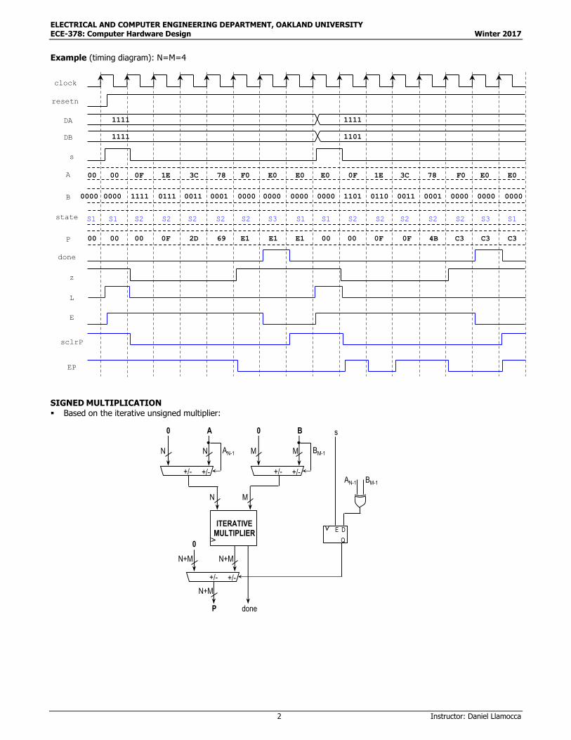
Iterative Multiplier Architecture (N-bit by M-bit): FSM + Datapath circuit.
𝑠𝑐𝑙𝑟: synchronous clear. In this case, if 𝑠𝑐𝑙𝑟 = 1 and 𝐸 = 1, the register contents are initialized to 0.
The solution is computed in 𝑀 + 1 cycles.
1 1 1 1 x
1 1 0 1
1 1 1 1
0 0 0 0
1 1 1 1
1 1 1 1
1 1 0 0 0 0 1 1
P 0 + 1111
P 1111
P 1111 + 111100 = 1001011
P 1001011 + 1111000 = 11000011
A
din
s_l
E
0
L
E
Parallel Access
s_l = 1 Load
s_l = 0 Shift
N+Mresetn
B
din
s_l
E
0
L
E
DataB
M
z b0
+
PE
sclr
EP
sclrP
FSM
s
done
sclrP
z
b0
EPE L
Shift-rightShift-left
S1
S2
resetn=0
1
0s
z
sclrP 1
EP 1
E 1
01
EP 1
1
0b0
S3
done 1
1s
0
L, E 1
N+M
N+M
N+M
M
DataAN
00..0
"00..0"&DataA
M
P
ELECTRICAL AND COMPUTER ENGINEERING DEPARTMENT, OAKLAND UNIVERSITY ECE-378: Computer Hardware Design Winter 2017
2 Instructor: Daniel Llamocca
Example (timing diagram): N=M=4
SIGNED MULTIPLICATION Based on the iterative unsigned multiplier:
clock
resetn
s
DB 11011111
DA 11111111
S1 S1 S2 S2 S2 S2 S2 S3 S1 S1 S2 S2 S2 S2 S2 S3 S1
B
A 0F
z
0000 1E 3C 78 F0 E0
11110000 0000 0111 0011 0001 0000 0000
state
000000 0F 2D 69 E1P
done
L
E
E1
sclrP
EP
1101 0110 0011 0001 0000
0F 1E 3C 78 F0 E0
00 00 0F 0F 4B C3 C3 C3E1
0000 0000 0000 0000
E0 E0 E0
N
+/- +/-
N
0 A
M
+/- +/-
M
0 B
ITERATIVE MULTIPLIER
N M
N+M
+/- +/-
N+M
0
AN-1 BM-1
BM-1AN-1
Q
s
N+M
doneP
E D

ELECTRICAL AND COMPUTER ENGINEERING DEPARTMENT, OAKLAND UNIVERSITY ECE-378: Computer Hardware Design Winter 2017
3 Instructor: Daniel Llamocca
INTEGER/FX DIVISION UNSIGNED DIVISION Unsigned division: Iterative case
For the implementation, we follow the hand-division method. We grab bits of A one by one and compare it with the divisor. If the result is greater or equal than B, then we subtract B from it. On each iteration, we get one bit of 𝑄. The example
below shows the case where 𝐴 = 10001100; 𝐵 = 1001.
A: N=8 bits
B: M=4 bits
R: M=4 bits
Intermediate subtraction requires M+1 bits
Q: N=8 bits
A 10001100, B 1001, R 00000000
i = 7, a7 = 1: R 00001 < 1001 q7 = 0
i = 6, a6 = 0: R 00010 < 1001 q6 = 0
i = 5, a5 = 0: R 00100 < 1001 q5 = 0
i = 4, a4 = 0: R 01000 < 1001 q4 = 0
i = 3, a3 = 1: R 10001 1001 q3 = 1, R 10001 – 1001 = 01000
i = 2, a2 = 1: R 10001 1001 q2 = 1, R 10001 – 1001 = 01000
i = 1, a1 = 0: R 10000 1001 q1 = 1, R 10000 – 1001 = 00111
i = 0, a0 = 0: R 01110 1001 q0 = 1, R 01110 – 1001 = 00101
Q 00001111, R 0101
An iterative architecture is depicted in the figure for A with 𝑁 bits and B with 𝑀 bits, 𝑁 ≥ 𝑀. The register 𝑅 stores the
remainder. At every clock cycle, we either: i) shift in the next bit of A, or ii) shift in the next bit of A and subtract B. (𝑀 + 1)-bit unsigned subtractor: We can apply 2C operation to B. If the subtraction is negative, 𝑐𝑜𝑢𝑡 = 0. If the subtraction
is positive, 𝑐𝑜𝑢𝑡 = 1 (here, we only need to capture 𝑅 with 𝑀 bits). This determines 𝑞𝑖, which is shifted into the register A,
which after 𝑁 cycles holds 𝑄.
00001111
10001100
1001
10001
1001
10000
1001
1110
1001
101
1001 AB
Q
R
ALGORITHM
R = 0
for i = N-1 downto 0
left shift R (input = ai)
if R B
qi = 1, R R-B
else
qi = 0
end
end
15
140
90
50
45
5
9 AB
Q
R
aN-1
M+1
LEFT SHIFT
REGISTER
s_LE w REGISTER
E
DA DB
+cout
Q
B
LEFT SHIFT
REGISTER
sclrs_LE
w
MN
M
M+1
0&B
R
M
A
aN-1
M+1
0
M
RM-1RM-2...R0aN-1
RM-1RM-2...R0
E
FSM
sclrRLRER
done
LAB
EA
MN
cout
cout
M
Y
sclrR 1, ER1
C 0
S1
1
resetn=0
E0
ER 1, EA 1
S2
done 1
S3
1cout
0
0C=N-1 C C+1
1
LAB, EA 1
LR 1
E10
clock
resetn
TMTM-1...T0
cin 1
TM-1...T0

ELECTRICAL AND COMPUTER ENGINEERING DEPARTMENT, OAKLAND UNIVERSITY ECE-378: Computer Hardware Design Winter 2017
4 Instructor: Daniel Llamocca
Example (timing diagram 𝑁 = 5, 𝑀 = 4). i) DA = 27, DB = 9, ii) DA = 20, DB = 7
SIGNED MULTIPLICATION Based on the iterative unsigned multiplier
Signed division: In this case, we first take the absolute value of the operators A and B. Depending on the sign of these operators, the division result (positive) of abs(A)/abs(B) might require a sign change.
clock
resetn
EA
EC
QC
zC
cout
LR
ER
state
done
E
Q
DB 01111001 0011
00000
R 0000
DA 1010011011 00000
000
T 00000
00000 11011 10110 01100 11000 10001 00011
000
S1 S1 S2
000
S2
001 010 011 100
S2 S2 S2 S3 S1 S1
100 100 000 000
S2 S2
001 010 011 100
S2 S2 S2 S3
100
S1
100
0000 0000 0001 0011 0110 0100 0000
101110000000000 11000 11010 11101 00100
00011
0000
10111
00011
0000
10111
0000
10100
11010
01000
0001
11011
10000
0010
11110
00000
0101
00011
00001
0011
11111
00010
0110
00101
00010
0110
00101
N
+/- +/-
N
0 A
M
+/- +/-
M
0 B
ITERATIVE DIVIDER
N M
N
+/- +/-
N
0
AN-1 BM-1
BM-1AN-1
Q
s
N
doneP
E D

ELECTRICAL AND COMPUTER ENGINEERING DEPARTMENT, OAKLAND UNIVERSITY ECE-378: Computer Hardware Design Winter 2017
5 Instructor: Daniel Llamocca
INTEGER/FX ACCUMULATOR DIGITAL SYSTEM (FSM + Datapath circuit) sclr: Synchronous clear. If E = ‘1’ and sclr = ‘1’, then the output bits of the registers are set to zero.
Finite State Machine (FSM): Algorithmic State Machine (ASM):
E|restart/Ei|sclr
S1 S210/10
resetn = 0
X1/11
10/10
X1/11
00/0000/00
S1
S2
resetn=0
1
0E
0
restart1
Ei, sclr 1
Ei, sclr 1
Ei 1
E
Ei 1
1
0
0
restart1
QD
resetn
+
QD
20
2088
Dout
Din
FINITE STATE MACHINE
E
E sclr
restart
E
Ei
sclr
sign
extension
ELECTRICAL AND COMPUTER ENGINEERING DEPARTMENT, OAKLAND UNIVERSITY ECE-378: Computer Hardware Design Winter 2017
6 Instructor: Daniel Llamocca
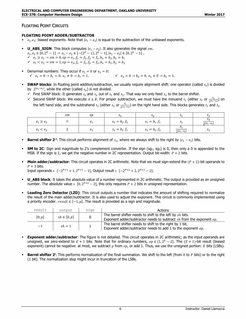
FLOATING POINT CIRCUITS FLOATING POINT ADDER/SUBTRACTOR 𝑒1, 𝑒2: biased exponents. Note that |𝑒1 − 𝑒2| is equal to the subtraction of the unbiased exponents.
U_ABS_SIGN: This block computes |𝑒1 − 𝑒2|. It also generates the signal 𝑠𝑚.
𝑒1, 𝑒2 ∈ [0, 2𝐸 − 1] → 𝑒1 − 𝑒2 ∈ [−(2𝐸 − 1), 2𝐸 − 1], |𝑒1 − 𝑒2| ∈ [0, 2𝐸 − 1] . 𝑒1 ≥ 𝑒2 → 𝑠𝑚 = 0, 𝑒𝑝 = 𝑒1, 𝑓𝑥 = 𝑓2, 𝑓𝑦 = 𝑓1, 𝑏𝑥 = 𝑏2, 𝑏𝑦 = 𝑏1
𝑒1 < 𝑒2 → 𝑠𝑚 = 1, 𝑒𝑝 = 𝑒2, 𝑓𝑥 = 𝑓1, 𝑓𝑦 = 𝑓2, 𝑏𝑥 = 𝑏1, 𝑏𝑦 = 𝑏2
Denormal numbers: They occur if 𝑒1 = 0 or 𝑒2 = 0:
𝑒1 = 0 → 𝑏1 = 0. 𝑒1 ≠ 0 → 𝑏1 = 1. 𝑒2 = 0 → 𝑏2 = 0. 𝑒2 ≠ 0 → 𝑏2 = 1.
SWAP blocks: In floating point addition/subtraction, we usually require alignment shift: one operator (called 𝑠𝑥) is divided
by 2|𝑒1−𝑒2|, while the other (called 𝑠𝑦) is not divided.
First SWAP block: It generates 𝑠𝑥 and 𝑠𝑦 out of 𝑠1 and 𝑠2. That way we only feed 𝑠𝑥 to the barrel shifter.
Second SWAP block: We execute 𝐴 ± 𝐵. For proper subtraction, we must have the minuend 𝑡1 (either 𝑠1 or 𝑠1
2|𝑒1−𝑒2|) on
the left hand side, and the subtrahend 𝑡2 (either 𝑠2 or 𝑠2
2|𝑒1−𝑒2|) on the right hand side. This blocks generates 𝑡1 and 𝑡2.
𝑠𝑚 𝑒𝑝 𝑠𝑥 𝑠𝑦 𝑡1 𝑡2
𝑒1 ≥ 𝑒2 0 𝑒1 𝑠2 = 𝑏2. 𝑓2 𝑠1 = 𝑏1. 𝑓1 𝑠1 𝑠2
2|𝑒1−𝑒2|
𝑒1 < 𝑒2 1 𝑒2 𝑠1 = 𝑏1. 𝑓1 𝑠2 = 𝑏2. 𝑓2 𝑠1
2|𝑒1−𝑒2| 𝑠2
Barrel shifter 2-i: This circuit performs alignment of 𝑠𝑥, where we always shift to the right by |𝑒1 − 𝑒2| bits.
SM to 2C: Sign and magnitude to 2’s complement converter. If the sign (sg1, sg2) is 0, then only a 0 is appended to the
MSB. If the sign is 1, we get the negative number in 2C representation. Output bit-width: 𝑃 + 2 bits.
Main adder/subtractor: This circuit operates in 2C arithmetic. Note that we must sign-extend the (𝑃 + 2)-bit operands to
𝑃 + 3 bits.
Input operands [−2𝑃+1 + 1, 2𝑃+1 − 1], Output result [−2𝑃+2 + 2, 2𝑃+2 − 2]. U_ABS block: It takes the absolute value of a number represented in 2C arithmetic. The output is provided as an unsigned
number. The absolute value [0, 2𝑃+2 − 2], this only requires 𝑃 + 2 bits in unsigned representation.
Leading Zero Detector (LZD): This circuit outputs a number that indicates the amount of shifting required to normalize
the result of the main adder/subtractor. It is also used to adjust the exponent. This circuit is commonly implemented using a priority encoder. 𝑟𝑒𝑠𝑢𝑙𝑡 ∈ [−1, 𝑝]. The result is provided as a sign and magnitude.
result output sign Actions
[0, 𝑝] 𝑠ℎ ∈ [0, 𝑝] 0 The barrel shifter needs to shift to the left by 𝑠ℎ bits.
Exponent adder/subtractor needs to subtract 𝑠ℎ from the exponent 𝑒𝑝.
−1 𝑠ℎ = 1 1 The barrel shifter needs to shift to the right by 1 bit. Exponent adder/subtractor needs to add 1 to the exponent 𝑒𝑝.
Exponent adder/subtractor: The figure is not detailed. This circuit operates in 2C arithmetic; as the input operands are
unsigned, we zero-extend to 𝐸 + 1 bits. Note that for ordinary numbers, 𝑒𝑝 ∈ [1, 2𝐸 − 2]. The (𝐸 + 1)-bit result (biased
exponent) cannot be negative: at most, we subtract 𝑝 from 𝑒𝑝, or add 1. Thus, we use the unsigned portion: 𝐸 bits (LSBs).
Barrel shifter 2i: This performs normalization of the final summation. We shift to the left (from 0 to 𝑃 bits) or to the right
(1 bit). The normalization step might incur in truncation of the LSBs.

ELECTRICAL AND COMPUTER ENGINEERING DEPARTMENT, OAKLAND UNIVERSITY ECE-378: Computer Hardware Design Winter 2017
7 Instructor: Daniel Llamocca
This circuit works for ordinary numbers. 𝑁𝑎𝑁, ±∞: not considered.
Denormal numbers: not implemented: this would require |𝑒1 − 𝑒2| = |1 − 𝑒2| when 𝑒1 = 0, or |𝑒1 − 1| when 𝑒2 = 0. But we implement 𝐴 ± 𝐵 when 𝐴 = 0, 𝐵 = 0, 𝐴 = 𝐵 = 0.
If 𝐴 = 0 or 𝐵 = 0, then 𝑠𝑥 = 0 (barrel shifter input). So, the incorrect |𝑒1 − 𝑒2| does not matter; 𝑒𝑝 will also be correct.
As for the biased exponent 𝑒, if 𝑡1 ± 𝑡2 = 0, then 𝐴 ± 𝐵 = 0, and we must make 𝑒 = 0 (we use a multiplexer here). After normalization, the unbiased 𝑒 might be 2𝐸 − 1. This indicates overflow, but we would need to make 𝑓 = 0. We do
not implement this, so overflow is not detected. Typical cases:
Single Precision: E = 8, P = 23. Double Precision: E = 8, P = 52.
E
EE
e1 e2
PPfX fY
P+1
sX
P+1
sY
bX
2-i
SM to 2C
sg1 sg2
P+2 P+2
+/-+/-
add/sub
U_ABS_SIGN
U_ABS
P+3
P+2
2i
P+2
s
sg
MSB
LZD
E ex
P
f
sm
ep
...
E
dir
+/-
SM to 2C
01 10
f1 f2
P P
01 10
P+1 P+1
E
e1 f1sg1
e2 f2sg2
e fsg
±
P+1 P+1
1
32 bits
FPadd/sub
32
A B
32
32
S
A
B
S
add/sub
0: +
1: -
10
...
...
bY
SWAP
SWAP
bX
01 10
b1 b2
bY
sm
e1 0 e2 0
EE
e1 e2
01
e
E
0
Q =0
P+2

ELECTRICAL AND COMPUTER ENGINEERING DEPARTMENT, OAKLAND UNIVERSITY ECE-378: Computer Hardware Design Winter 2017
8 Instructor: Daniel Llamocca
FLOATING POINT MULTIPLIER AND DIVIDER Multiplier: An unsigned multiplier is required. If we use a sequential multiplier, an FSM is required to control the dataflow.
We need to add the unbiased exponents: 𝑒𝑝 = 𝑒1 + 𝑒2. Here, a simple unsigned adder suffices. Since this operation adds
2 × 𝑏𝑖𝑎𝑠 to ep, we subtract bias from the final adjusted exponent 𝑒𝑥.
The multiplier will require 2P+2 bits. Here, we need to truncate to P+2 bits. Divider: An unsigned divider is required. If we use a sequential divider, an FSM is required to control the dataflow.
We need to subtract the unbiased exponents: 𝑒𝑝 = 𝑒1 − 𝑒2. This requires us to operate in 2C arithmetic. Since this
operation gets rid of the bias, we need to add the 𝑏𝑖𝑎𝑠 = 2𝐸−1 − 1 to the final adjusted exponent 𝑒𝑥.
The divider can include any number of extra fractional bits. We use P fractional bits of precision.
EE
e1 e2
PP
f1 f2
P+1s1
P+1s2
1 1
2P+2
sg
...
+
E+1
sg1 sg2
EE
e1 e2
PP
f1 f2
P+1s1
P+1s2
1 1
sg
-
E+1
sg1 sg2
DIVIDERwith P
fractional bits
FP MULTIPLIER FP DIVIDER
2i
P+2
LZD
P
f
dir
+/-
...
...
...P+2
Ee
-
E+1 bias
epep
s
2i
P+2
LZD
P
f
dir
+/-
...
...
...P+1
Ee
-
E+1 biass
ex ex
unsigned signed

ELECTRICAL AND COMPUTER ENGINEERING DEPARTMENT, OAKLAND UNIVERSITY ECE-378: Computer Hardware Design Winter 2017
9 Instructor: Daniel Llamocca
CORDIC (COORDINATE ROTATION DIGITAL COMPUTER) ALGORITHM CIRCULAR CORDIC The original circular CORDIC algorithm is described by the following iterative equations, where 𝑖 is the index of the iteration
(𝑖 = 0, 1, 2, 3, …). Depending on the mode of operation, the value of 𝛿𝑖 is either +1 or –1:
𝑥𝑖+1 = 𝑥𝑖 + 𝑖𝑦𝑖2−𝑖
𝑦𝑖+1 = 𝑦𝑖 − 𝑖𝑥𝑖2−𝑖
𝑧𝑖+1 = 𝑧𝑖 + 𝑖𝑖 , 𝑖 = 𝑇𝑎𝑛−1(2−𝑖)
𝑅𝑜𝑡𝑎𝑡𝑖𝑜𝑛: 𝛿𝑖 = +1 𝑖𝑓 𝑧𝑖 < 0; −1, 𝑜𝑡ℎ𝑒𝑟𝑤𝑖𝑠𝑒𝑉𝑒𝑐𝑡𝑜𝑟𝑖𝑛𝑔: 𝛿𝑖 = +1 𝑖𝑓 𝑦𝑖 ≥ 0; −1, 𝑜𝑡ℎ𝑒𝑟𝑤𝑖𝑠𝑒
Depending on the mode of operation, the quantities X, Y and Z tend to the following values, for sufficiently large 𝑁:
Rotation Mode Vectoring Mode
𝑥𝑛 = 𝐴𝑛(𝑥0𝑐𝑜𝑠𝑧0 − 𝑦0𝑠𝑖𝑛𝑧0)
𝑦𝑛 = 𝐴𝑛(𝑦0𝑐𝑜𝑠𝑧0 + 𝑥0𝑠𝑖𝑛𝑧0)
𝑧𝑛 = 0
𝑥𝑛 = 𝐴𝑛√𝑥02 + 𝑦0
2
𝑦𝑛 = 0
𝑧𝑛 = 𝑧0 + 𝑡𝑎𝑛−1(𝑦0 𝑥0⁄ )
𝐴𝑛 ← ∏ √1 + 2−2𝑖𝑁−1𝑖=0 . For 𝑁 →∝ , 𝐴𝑛 = 1.647. The 𝑡𝑎𝑛−1 function here has a different definition, as the values it compute
lie in the range [−180°, 180°], i.e., it indicates the quadrant where the point (𝑥0, 𝑦0) lies.
With a proper choice of the initial values 𝑥0, 𝑦0, 𝑧0 and the operation mode, the following functions can be directly computed:
𝑦0 = 0, 𝑥0 = 1 𝐴𝑛⁄ , rotation mode 𝑥𝑛 = 𝑐𝑜𝑠𝑧0, 𝑦𝑛 = 𝑠𝑖𝑛𝑧0
𝑧0 = 0, 𝑥0 = 1, vectoring mode 𝑧𝑛 = 𝑡𝑎𝑛−1(𝑦0)
𝑥0 = 𝑎, 𝑦0 = 𝑏, vectoring mode 𝑥𝑛 = 𝐴𝑛√𝑎2 + 𝑏2. We need to post-scale the output.
LINEAR CORDIC This is an extension to the circular CORDIC. No scaling corrections are needed. (𝑖 = 1, 2, 3, …).
𝑥𝑖+1 = 𝑥𝑖
𝑦𝑖+1 = 𝑦𝑖 − 𝑖𝑥𝑖2−𝑖
𝑧𝑖+1 = 𝑧𝑖 + 𝑖𝑖 , 𝑖 = 2−𝑖
𝑅𝑜𝑡𝑎𝑡𝑖𝑜𝑛: 𝛿𝑖 = +1 𝑖𝑓 𝑧𝑖 < 0; −1, 𝑜𝑡ℎ𝑒𝑟𝑤𝑖𝑠𝑒𝑉𝑒𝑐𝑡𝑜𝑟𝑖𝑛𝑔: 𝛿𝑖 = +1 𝑖𝑓 𝑥𝑖𝑦𝑖 ≥ 0; −1, 𝑜𝑡ℎ𝑒𝑟𝑤𝑖𝑠𝑒
Depending on the mode of operation, the quantities X, Y and Z tend to the following values, for sufficiently large 𝑁:
Rotation Mode Vectoring Mode
𝑥𝑛 = 𝑥1
𝑦𝑛 = 𝑦1 + 𝑥1𝑧1
𝑧𝑛 = 0
𝑥𝑛 = 𝑥1
𝑦𝑛 = 0
𝑧𝑛 = 𝑧1 + 𝑦1 𝑥1⁄
With a proper choice of the initial values 𝑥0, 𝑦0, 𝑧0 and the operation mode, the following functions can be directly computed:
𝑦1 = 0, rotation mode 𝑦𝑛 = 𝑥1𝑧1
𝑧1 = 0, vectoring mode 𝑧𝑛 = 𝑦1 𝑥1⁄
HYPERBOLIC CORDIC This extension to the original CORDIC equations allows for the computation of hyperbolic functions, where 𝑖 is the index of
the iteration (𝑖 = 1, 2, 3, …). The following iterations must be repeated to guarantee convergence: 𝑖 = 4, 13, 40, … , 𝑘, 3𝑘 + 1.
𝑥𝑖+1 = 𝑥𝑖 − 𝑖𝑥𝑖2−𝑖
𝑦𝑖+1 = 𝑦𝑖 − 𝑖𝑥𝑖2−𝑖
𝑧𝑖+1 = 𝑧𝑖 + 𝑖𝑖 , 𝑖 = 𝑡𝑎𝑛ℎ−1(2−𝑖)
𝑅𝑜𝑡𝑎𝑡𝑖𝑜𝑛: 𝛿𝑖 = +1 𝑖𝑓 𝑧𝑖 < 0; −1, 𝑜𝑡ℎ𝑒𝑟𝑤𝑖𝑠𝑒𝑉𝑒𝑐𝑡𝑜𝑟𝑖𝑛𝑔: 𝛿𝑖 = +1 𝑖𝑓 𝑥𝑖𝑦𝑖 ≥ 0; −1, 𝑜𝑡ℎ𝑒𝑟𝑤𝑖𝑠𝑒
Depending on the mode of operation, the quantities X, Y and Z tend to the following values, for sufficiently large 𝑁:
Rotation Mode Vectoring Mode
𝑥𝑛 = 𝐴𝑛(𝑥1𝑐𝑜𝑠ℎ𝑧1 + 𝑦1𝑠𝑖𝑛ℎ𝑧1)
𝑦𝑛 = 𝐴𝑛(𝑦1𝑐𝑜𝑠ℎ𝑧1 + 𝑥1𝑠𝑖𝑛ℎ𝑧1)
𝑧𝑛 = 0
𝑥𝑛 = 𝐴𝑛√𝑥12 − 𝑦1
2
𝑦𝑛 = 0
𝑧𝑛 = 𝑧1 + 𝑡𝑎𝑛ℎ−1(𝑦1 𝑥1⁄ )
𝐴𝑛 ← ∏ √1 − 2−2𝑖𝑁𝑖=1 (this includes the repeated iterations 𝑖 = 4, 13, 40, …,). For 𝑁 →∝ , 𝐴𝑛 ≅ 0.8
With a proper choice of the initial values 𝑥1, 𝑦1, 𝑧1 and the operation mode, the following functions can be directly computed:
𝑦1 = 0, 𝑥1 = 1 𝐴𝑛⁄ , rotation mode 𝑥𝑛 = 𝑐𝑜𝑠ℎ𝑧1, 𝑦𝑛 = 𝑠𝑖𝑛ℎ𝑧1
𝑧1 = 0, 𝑥1 = 1, vectoring mode 𝑧𝑛 = 𝑡𝑎𝑛ℎ−1(𝑦1) 𝑥1 = 𝑦1 = 1 𝐴𝑛⁄ , rotation mode 𝑥𝑛 = 𝑦𝑛 = 𝑐𝑜𝑠ℎ𝑧1 + 𝑠𝑖𝑛ℎ𝑧1 = 𝑒𝑧1
𝑥1 = 𝛼 + 1, 𝑦1 = 𝛼 − 1, 𝑧1 = 0, vectoring mode 𝑧𝑛 = 𝑡𝑎𝑛ℎ−1(𝛼 − 1 𝛼 + 1⁄ ) = (ln 𝛼) 2⁄ .
𝑥1 = 𝛼 + 1 (4𝐴𝑛2 )⁄ , 𝑦1 = 𝛼 − 1 (4𝐴𝑛
2 )⁄ , 𝑧1 = 0, vectoring mode 𝑥𝑛 = √𝛼

ELECTRICAL AND COMPUTER ENGINEERING DEPARTMENT, OAKLAND UNIVERSITY ECE-378: Computer Hardware Design Winter 2017
10 Instructor: Daniel Llamocca
RANGE OF CONVERGENCE The basic range of convergence, obtained by a method developed by X. Hu et al, “Expanding the Range of Convergence of
the CORDIC Algorithm”, results:
Rotation Mode: |𝑧𝑖𝑛| ≤ 𝜃𝑁 + ∑ 𝜃𝑖
𝑁
𝑖=𝑖𝑖𝑛
Circular: 𝑖𝑖𝑛 = 0, 𝑧𝑖𝑛 = 𝑧0, 𝛼𝑖𝑛 = 𝑡𝑎𝑛−1(𝑦0
𝑥0⁄ )
Linear: 𝑖𝑖𝑛 = 1, 𝑧𝑖𝑛 = 𝑧1, 𝛼𝑖𝑛 =𝑦1
𝑥1⁄
Hyperbolic: 𝑖𝑖𝑛 = 1, 𝑧𝑖𝑛 = 𝑧1, 𝛼𝑖𝑛 = 𝑡𝑎𝑛ℎ−1(𝑦1
𝑥1⁄ ). Note that in
the summation, we must repeat the terms 𝑖 = 4, 13, 40, Vectoring Mode: |𝛼𝑖𝑛| ≤ 𝜃𝑁 + ∑ 𝜃𝑖
𝑁
𝑖=𝑖𝑖𝑛
Circular:
𝜃𝑁 + ∑ 𝜃𝑖
𝑁
𝑖=0
= 𝑡𝑎𝑛−1(2−𝑁) + ∑ 𝑡𝑎𝑛−1(2−𝑖)
𝑁
𝑖=0
= 1.7433 (𝑁 → ∞)
Rotation |𝑧0| ≤ 1.7433 (99.9°) Input angle 𝜖 [−99.9°, 99.9°]. Functions with
angles outside this range can be computed by
applying trigonometric identities.
Vectoring |𝑡𝑎𝑛−1(𝑦0
𝑥0⁄ )| ≤ 1.7433 (99.9°) →
𝑦0𝑥0
⁄ 𝜖⟨−∞, ∞⟩ There are no restrictions on the ratio
𝑦0𝑥0
⁄ .
However, we cannot compute the angle for values outside the range [−99.9°, 99.9°].
Linear:
𝜃𝑁 + ∑ 𝜃𝑖
𝑁
𝑖=1
= 2−𝑁 + ∑ 2−𝑖
𝑁
𝑖=1
= 1
Rotation |𝑧1| ≤ 1 In both cases, there is a strict limitation on the input argument of the linear function (e.g. multiplication, division)
Vectoring |𝑦1
𝑥1⁄ | ≤ 1
Hyperbolic:
𝜃𝑁 + ∑ 𝜃𝑖
𝑁
𝑖=1
= 𝑡𝑎𝑛ℎ−1(2−𝑁) + ∑ 𝑡𝑎𝑛ℎ−1(2−𝑖)
𝑁
𝑖=1
= 1.182 (𝑁 → ∞)
Rotation |𝑧1| ≤ 1.182 This is the limitation imposed to the input argument of the hyperbolic functions. Note that the full domain of the functions 𝑠𝑖𝑛ℎ and 𝑐𝑜𝑠ℎ is ⟨−∝, ∝⟩.
Vectoring |𝑡𝑎𝑛ℎ−1(𝑦1
𝑥1⁄ )| ≤ 1.182 → |
𝑦1𝑥1
⁄ | ≤ 0.807 This is the limitation imposed to the ratio of the input arguments of the hyperbolic functions. Note that the domain of 𝑡𝑎𝑛ℎ−1 is ⟨−1,1⟩.
ITERATIVE ARCHITECTURE The architecture is such that the inputs and outputs have an identical bit width. We can reach an optimal number of iterations
by noticing the iteration at which 𝑖 = 𝑇𝑎𝑛−1(2−𝑖) is equal to zero due to for a particular fixed-point representation.
𝑛: input/output bit width
𝑛𝑔: additional guard bits on the LSB.
𝑛𝑟: 𝑛𝑟 = 𝑛𝑔 + 𝑛 : bit width of the internal registers and operators
𝑁: number of iterations (𝑖 = 0,1, … , 𝑁 for circular CORDIC, 𝑖 = 1, … , 𝑁 for linear/hyperbolic CORDIC) 𝑥𝑖 , 𝑦𝑖 , 𝑧𝑖 may require more bits than the final values. A common rule of thumb is “If 𝑛 bits is the desired output precision, the
internal registers should have ⌈log2 𝑛⌉ additional guard bits at the LSB position”. A more accurate procedure is to perform
software simulation for a given number of iterations and find out the number of bits required for proper representation of the 𝑥𝑖 , 𝑦𝑖 , 𝑧𝑖 quantities.
Circular CORDIC The figure below depicts the architecture that implements the circular CORDIC equations in an iterative fashion. The LUT
(look-up table) is needed to store the sets of elementary angles 𝑖 = 𝑇𝑎𝑛−1(2−𝑖). The process begins when a start signal is
asserted. After 𝑁 clock cycles, the result is obtained in the registers X, Y and Z, and a new process can be started.
A state machine, which controls the load of the registers, the data that passes onto the multiplexers, the add/subtract decision for the adder/subtractors, and the count given to the barrel shifters and LUT.

ELECTRICAL AND COMPUTER ENGINEERING DEPARTMENT, OAKLAND UNIVERSITY ECE-378: Computer Hardware Design Winter 2017
11 Instructor: Daniel Llamocca
Hyperbolic CORDIC
Here the LUT holds the 𝑖 = 𝑡𝑎𝑛ℎ−1(2−𝑖) values with 𝑖 = 1,2, … , 𝑁. The FSM is more complex as it has to account for the
repeated iterations. After 𝑁 − 1 + 𝑣 (𝑣: # of repeated iterations) clock cycles, the result is obtained in the registers X, Y and
Z, and a new process can be started.
0 1 1 0
nr
ng0
n
Xin
nr
ng0
n
Yin
E E
2-i
s_xyz
E
+/-
i
data_X data_Y
X Y
di
next_X next_Y
n
X_out Y_out
0 1
n
Zin
E
data_Z
Z
next_Z
Z_out
n
Tan-1(2-i)
i
e_i
LUT
di
FSMY
Z
s mode
done
di
s_xyz
E i
n n
+/- +/-
E E
s_xyz
0 1 1 0
nr
ng0
n
Xin
nr
ng0
n
Yin
2-i
s_xyz
+/-
i
data_X data_Y
X Y
di
next_X next_Y
n
X_out Y_out
0 1
n
Zin
data_Z
Z
next_Z
Z_out
n
Tanh-1(2-i)
i
e_i
LUT
di
FSMY
Z
s mode
done
di
s_xyz
E i
n n
+/- +/-
X
E EE
EE E
s_xyz

ELECTRICAL AND COMPUTER ENGINEERING DEPARTMENT, OAKLAND UNIVERSITY ECE-378: Computer Hardware Design Winter 2017
12 Instructor: Daniel Llamocca
Linear CORDIC Here the LUT holds the 𝑖 = 2−𝑖 values with 𝑖 = 1,2, … , 𝑁. After 𝑁 − 1 clock cycles, the result is obtained in the registers X,
Y and Z, and a new process can be started. Note that we do not need an adder for 𝑥𝑖.
Note that the architectures do not specify the numerical format we are using. We are free to use any format we desire (e.g.: fixed point, dual fixed point, floating point). The adders, barrel shifters, and LUT will change depending on the desired format. If an arithmetic unit requires more than one cycle to process its date, the FSM needs to account for this.
1 0
nr
ng0
n
Xin
nr
ng0
n
Yin
2-i
s_yz
i
data_X data_Y
X Y
di
next_X
next_Y
n
X_out Y_out
0 1
n
Zin
data_Z
Z
next_Z
Z_out
n
2-i
i
e_i
LUT
di
FSMY
Z
s mode
done
di
s_yz
E i
n n
+/- +/-
X
E EE
EE E
s_yz

ELECTRICAL AND COMPUTER ENGINEERING DEPARTMENT, OAKLAND UNIVERSITY ECE-378: Computer Hardware Design Winter 2017
13 Instructor: Daniel Llamocca
Example: FX CORDIC with [16 14]
0 1 1 0
40
16
Xin
40
16
Yin
E E
2-i
s_xyz
E
+/-
i
data_X data_Y
X Y
di
next_X next_Y
Xout Yout
0 1
16
Zin
E
data_Z
Z
next_Z
Zout
16
Tan-1(2-i)
i
e_i
LUT
di
CTRLY
Z
s mode
done
di
s_xyz
E i
+/- +/-
E E
16 16 16
2020
16
20 20
2020 20 20
16
20 20
s_xyz
FSM
Q
counter
0 to 15
E
sclr z
Ei
sclri
s
4 i
zi
D
E
Q
s_xyz
mode
Z(15)Y(19)
1 0
di
E
CTRL
resetn=0
1
Ei, sclri 1
s
S2
S2
s_xyz 1
E 1
E 1
0
1
zi Ei 1
Ei, sclri 1
FSM
1
done 1
s
S3
0
0

ELECTRICAL AND COMPUTER ENGINEERING DEPARTMENT, OAKLAND UNIVERSITY ECE-378: Computer Hardware Design Winter 2017
14 Instructor: Daniel Llamocca
FIXED-POINT SQUARE ROOT Algorithms for hardware implementation amount to a ‘binary search’ and can be classified as Restoring and Non-Restoring.
𝐷 (radical): 2𝑛 bits, 𝑄 (square root): 𝑛 bits.
Restoring Algorithm Non-Restoring Algorithm 𝑄 ← 0 𝑓𝑜𝑟 𝑘 = 𝑛 − 1 → 0
𝑞𝑘 ← 1 𝑖𝑓 𝐷 < 𝑄2 𝑡ℎ𝑒𝑛
𝑞𝑘 ← 0 𝑒𝑛𝑑
𝑒𝑛𝑑
𝑞𝑛−1 ← 1 𝑓𝑜𝑟 𝑘 = 𝑛 − 2 → 0
𝑖𝑓 𝐷 < 𝑄2 𝑡ℎ𝑒𝑛 𝑄 ← 𝑄 − 2𝑘
𝑒𝑙𝑠𝑒
𝑄 ← 𝑄 + 2𝑘 𝑒𝑛𝑑
𝑒𝑛𝑑
Example: 𝐷 = 40 = 101000, 𝑄 = 000, 𝑛 = 3 𝑘 = 2: 𝑞2 = 1 (𝑄 = 100)
40 < 42? 𝑁𝑜 𝑘 = 1: 𝑞1 = 1 (𝑄 = 110)
40 < 62? 𝑁𝑜 𝑘 = 0: 𝑞0 = 1 (𝑄 = 111)
40 < 72? 𝑌𝑒𝑠 → 𝑞0 = 0 (𝑄 = 110) Result: 𝑄 = 110, 𝑅 = 𝐷 − 𝑄2 = 0100
Example: 𝐷 = 40 = 101000, 𝑛 = 3 𝑞2 = 1 (𝑄 = 100) 𝑘 = 1: 40 < 42? 𝑁𝑜 𝑄 ← 𝑄 + 21 = 110 𝑘 = 0: 40 < 62? 𝑁𝑜 𝑄 ← 𝑄 + 20 = 111
Result: 𝑄 = 111, 𝑅 = 𝐷 − 𝑄2? The LSB of the result might
differ from that of the restoring case. Also, the remainder might be incorrect when using this algorithm.
OPTIMIZED NON-RESTORING INTEGER SQRT ALGORITHM This algorithm for non-restoring square root VLSI implementation, described in A New Non-Restoring Square Root Algorithm
and its VLSI Implementation”, Y. Li, W. Chu, 1996, has proved to outperform most hardware algorithms. A simple addition and subtraction is required based on the result bit generated in the previous iteration. No multipliers or multiplexors are needed. The result of the addition or subtraction is fed via registers to the next iteration directly even if it is negative.
At the last iteration, if the remainder is non-negative, it is the precise remainder. Otherwise, we can get the precise remainder by an addition operation, but since it is rarely used, it is dismissed in order to reduce resource consumption.
Radical: 𝐷 = 𝑑2𝑛−1𝑑2𝑛−2𝑑2𝑛−3𝑑2𝑛−4 … 𝑑1𝑑0 Square Root: 𝑄 = 𝑞𝑛−1𝑞𝑛−2 … 𝑞0 We define: 𝐷𝑘 = 𝑑2𝑛−1𝑑2𝑛−2 … 𝑑𝑘 , 𝑘 = 0,1, … , 𝑛 − 1. 𝐷2𝑘 has 2(𝑛 − 𝑘) bits.
𝑄𝑘 = 𝑞𝑛−1𝑞𝑛−2 … 𝑞𝑘 , 𝑘 = 0,1, … , 𝑛 − 1 𝑄𝑘 has 𝑛 − 𝑘 bits.
𝑓𝑜𝑟 𝑘 = 𝑛 − 1 𝑑𝑜𝑤𝑛𝑡𝑜 0 𝑖𝑓 𝑘 = 𝑛 − 1 𝑡ℎ𝑒𝑛
𝑅′𝑘 = 𝑑2𝑘+1𝑑2𝑘 − 01 (𝑅′𝑛−1 = 𝑑2𝑛−1𝑑2𝑛−2 − 01) 𝑒𝑙𝑠𝑒
𝑅′𝑘 = {𝑅′𝑘+1𝑑2𝑘+1𝑑2𝑘 − 𝑄𝑘+101, 𝑖𝑓𝑞𝑘+1 = 1
𝑅′𝑘+1𝑑2𝑘+1𝑑2𝑘 + 𝑄𝑘+111, 𝑖𝑓𝑞𝑘+1 = 0
𝑒𝑛𝑑
𝑞𝑘 = {1, 𝑖𝑓 𝑅′𝑘 ≥ 0
0, 𝑖𝑓 𝑅′𝑘 < 0
𝑒𝑛𝑑
𝑅𝑒𝑚𝑎𝑖𝑛𝑑𝑒𝑟 𝑅 = 𝑅0 = {𝑅′0 𝑖𝑓 𝑅′0 ≥ 0
𝑅′0 + 𝑄101, 𝑖𝑓 𝑅′0 < 0
Estimated remainder: 𝑅′𝑘 = 𝑟′𝑛𝑟′𝑛−1𝑟′𝑛−2 … 𝑟′𝑘 (requires 𝑛 − 𝑘 + 1 bits) The MSB (sign bit) determines the value of 𝑞𝑘 (𝑞𝑘 is
computed at each iteration). The 𝑅′𝑘 value generated at each iteration is used in the next iteration even if it is negative (the
2C representation is used here). Note that the operands are always treated as unsigned numbers. Finally, in order to get the actual remainder 𝑅 = 𝑅0, only the 𝑛 + 1 LSBs of 𝑅′0 are needed (the MSB determines 𝑞0). In
practice, the remainder is seldom needed. Example: 𝐷 = 0111111, 𝑛 = 4, 𝑅 = 00000, 𝑄 = 0000 𝑘 = 𝑛 − 1 = 3: 𝑅’3 = 01 – 01 = 00 , 𝑅’3 = 𝑟′4𝑟′3 = 00, 𝑟’3 ≥ 0 → 𝑞3 = 1 𝑄 = 1000 𝑘 = 𝑛 − 2 = 2: 𝑅’2 = 𝑅’311 − 𝑄301 = 0011 − 0101 = −10 , 𝑅’2 = 𝑟′4𝑟′3𝑟′2 = 110, 𝑅’2 < 0 → 𝑞2 = 0 𝑄 = 1000
When the subtraction result is < 0, we use the 2C representation with 𝑛 − 𝑘 + 1 bits. The sign bit decides the value of 𝑞𝑘. 𝑘 = 1: 𝑅’1 = 𝑅’211 + 𝑄211 = 11011 + 1011 = 100110 , 𝑅’1 = 𝑟′4𝑟′3𝑟′2𝑟′1 = 0110, 𝑅′1 ≥ 0 → 𝑞1 = 1 𝑄 = 1010 𝑘 = 0: 𝑅’0 = 𝑅’111 − 𝑄101 = 011011 − 10101 = 00110 , 𝑅’0 = 𝑟′4𝑟′3𝑟′2𝑟′1𝑟′0 = 00110, 𝑅’0 ≥ 0 → 𝑞0 = 1 𝑄 = 1011 Also: 𝑅 = 𝑅’0 = 00110
ELECTRICAL AND COMPUTER ENGINEERING DEPARTMENT, OAKLAND UNIVERSITY ECE-378: Computer Hardware Design Winter 2017
15 Instructor: Daniel Llamocca
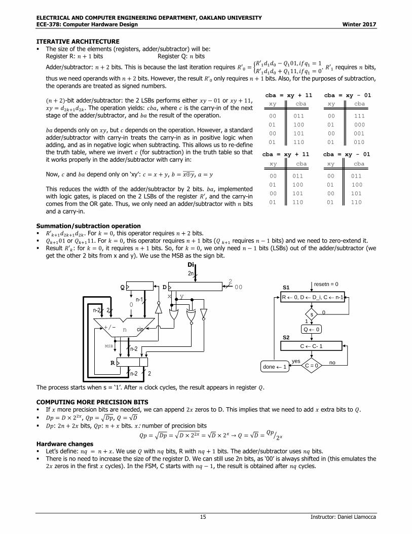
ITERATIVE ARCHITECTURE The size of the elements (registers, adder/subtractor) will be:
Register R: 𝑛 + 1 bits Register Q: 𝑛 bits
Adder/subtractor: 𝑛 + 2 bits. This is because the last iteration requires 𝑅′0 = {𝑅′1𝑑1𝑑0 − 𝑄101, 𝑖𝑓𝑞1 = 1
𝑅′1𝑑1𝑑0 + 𝑄111, 𝑖𝑓𝑞1 = 0. 𝑅′1 requires 𝑛 bits,
thus we need operands with 𝑛 + 2 bits. However, the result 𝑅’0 only requires 𝑛 + 1 bits. Also, for the purposes of subtraction,
the operands are treated as signed numbers.
(𝑛 + 2)-bit adder/subtractor: the 2 LSBs performs either 𝑥𝑦 − 01 or 𝑥𝑦 + 11,
𝑥𝑦 = 𝑑2𝑘+1𝑑2𝑘. The operation yields: 𝑐𝑏𝑎, where 𝑐 is the carry-in of the next
stage of the adder/subtractor, and 𝑏𝑎 the result of the operation.
𝑏𝑎 depends only on 𝑥𝑦, but 𝑐 depends on the operation. However, a standard
adder/subtractor with carry-in treats the carry-in as in positive logic when adding, and as in negative logic when subtracting. This allows us to re-define the truth table, where we invert 𝑐 (for subtraction) in the truth table so that
it works properly in the adder/subtractor with carry in: Now, 𝑐 and 𝑏𝑎 depend only on ‘xy’: 𝑐 = 𝑥 + 𝑦, 𝑏 = 𝑥𝑦̅̅ ̅̅ ̅̅ , 𝑎 = 𝑦
This reduces the width of the adder/subtractor by 2 bits. 𝑏𝑎, implemented with logic gates, is placed on the 2 LSBs of the register 𝑅′, and the carry-in
comes from the OR gate. Thus, we only need an adder/subtractor with 𝑛 bits
and a carry-in. Summation/subtraction operation 𝑅′𝑘+1𝑑2𝑘+1𝑑2𝑘. For 𝑘 = 0, this operator requires 𝑛 + 2 bits.
𝑄𝑘+101 or 𝑄𝑘+111. For 𝑘 = 0, this operator requires 𝑛 + 1 bits (𝑄 𝑘+1 requires 𝑛 − 1 bits) and we need to zero-extend it.
Result 𝑅′𝑘: for 𝑘 = 0, it requires 𝑛 + 1 bits. So, for 𝑘 = 0, we only need 𝑛 − 1 bits (LSBs) out of the adder/subtractor (we
get the other 2 bits from x and y). We use the MSB as the sign bit. The process starts when s = ‘1’. After 𝑛 clock cycles, the result appears in register 𝑄.
COMPUTING MORE PRECISION BITS If 𝑥 more precision bits are needed, we can append 2𝑥 zeros to D. This implies that we need to add 𝑥 extra bits to 𝑄.
𝐷𝑝 = 𝐷 × 22𝑥, 𝑄𝑝 = √𝐷𝑝, 𝑄 = √𝐷
𝐷𝑝: 2𝑛 + 2𝑥 bits, 𝑄𝑝: 𝑛 + 𝑥 bits. 𝑥: number of precision bits
𝑄𝑝 = √𝐷𝑝 = √𝐷 × 22𝑥 = √𝐷 × 2𝑥 → 𝑄 = √𝐷 =𝑄𝑝
2𝑥⁄
Hardware changes Let’s define: 𝑛𝑞 = 𝑛 + 𝑥. We use 𝑄 with 𝑛𝑞 bits, R with 𝑛𝑞 + 1 bits. The adder/subtractor uses 𝑛𝑞 bits.
There is no need to increase the size of the register D. We can still use 2n bits, as ‘00’ is always shifted in (this emulates the 2𝑥 zeros in the first 𝑥 cycles). In the FSM, C starts with 𝑛𝑞 − 1, the result is obtained after 𝑛𝑞 cycles.
xy
00
01
cba
cba = xy + 11
011
100
xy
00
01
cba
111
000
cba = xy - 01
00
01
101
110
00
01
001
010
xy
00
01
cba
cba = xy + 11
011
100
xy
00
01
cba
011
100
cba = xy - 01
00
01
101
110
00
01
101
110
+/-
0
n
MSBn-2
n-2
2
2
n-2
R
n-1
Q
x y
cin
002
D
Di
R 0, D D_i, C n-1
s
Q 0
C C- 1
resetn = 0S1
S2
yes no
1
0
done 1 C = 0
2n

ELECTRICAL AND COMPUTER ENGINEERING DEPARTMENT, OAKLAND UNIVERSITY ECE-378: Computer Hardware Design Winter 2017
16 Instructor: Daniel Llamocca
Example: (restoring algorithm)
Get √𝐷 using 𝑥 = 2 precision bits. 𝐷 = 110111 = 55, 𝑛 = 3
Then: 𝐷𝑝 = 1101110000 = 880. Then 𝑛𝑞 = 𝑛 + 𝑥 = 5
𝑘 = 4: 𝑞4 = 1 (𝑄 = 10000). 880 < 162? 𝑁𝑜
𝑘 = 3: 𝑞4 = 3 (𝑄 = 11000). 880 < 242? 𝑁𝑜
𝑘 = 2: 𝑞2 = 1 (𝑄 = 11100). 880 < 282? 𝑁𝑜 𝑘 = 1: 𝑞1 = 1 (𝑄 = 11110). 880 < 302? 𝑌𝑒𝑠 → 𝑞2 = 0 (𝑄 = 11100) 𝑘 = 0: 𝑞0 = 1 (𝑄 = 11101). 880 < 292? 𝑁𝑜
Result: 𝑄𝑝 = 11101, 𝑅𝑝 = 𝐷𝑝 − 𝑄𝑝2 = 100111
Final Result: 𝑄 = 111.01 = 7.25 ≈ √55
What if the input (let’s call it 𝑫𝒇) is in fixed-point format [𝟐𝒏 𝟐𝒑]?
The integer input (called 𝐷) is related to 𝐷𝑓 by: 𝐷𝑓 = 𝐷 × 2−2𝑝. 2𝑛 = number of total bits of 𝐷𝑓.
𝑄𝑓 = √𝐷𝑓 = √𝐷 × 2−2𝑝 = √𝐷 × 2−𝑝
So, we first compute the square root of 𝐷 (i.e., 𝐷𝑓 without the fractional point), and then we place the fractional point so
that the number has 𝑝 fractional bits.
If we need extra precision bits, we only need to add 2𝑥 zeros to 𝐷. Thus 𝐷𝑝 = 𝐷 × 22𝑥.
𝑄𝑓 = √𝐷𝑓 = √𝐷 × 2−𝑝 = √𝐷𝑝 × 2−2𝑥 × 2−𝑝 = √𝐷𝑝 × 2−𝑝−𝑥
Again, we first compute the square root of 𝐷𝑝, and then we place the fractional point so that the number 𝑄𝑓 has 𝑝 + 𝑥
fractional bits. Example (restoring algorithm)
𝐷𝑓 = 111011.1011 = 59.6875, 𝑝 = 2, 𝑛 = 5. Format [10 4]. 𝑄𝑓 format: [𝑛 + 𝑥 𝑝 + 𝑥]. 𝑥: extra precision bits.
Step 1: Get the integer D. 𝐷 = 1110111011 = 955
Step 2: Add (optionally) 2𝑥 = 4 zeros
𝐷𝑝 = 11101110110000 = 15280
Step 3: Get 𝑄𝑝 = √𝐷𝑝
Then: 𝐷𝑝 = 11101110110000 = 15280. Then 𝑛𝑞 = 𝑛 + 𝑥 = 5 + 2 = 7 𝑘 = 6: 𝑞6 = 1 (𝑄 = 1000000). 15280 < 642? 𝑁𝑜
𝑘 = 5: 𝑞5 = 1 (𝑄 = 1100000). 15280 < 962? 𝑁𝑜
𝑘 = 4: 𝑞4 = 1 (𝑄 = 1110000). 15280 < 1122? 𝑁𝑜 𝑘 = 3: 𝑞3 = 1 (𝑄 = 1111000). 15280 < 1202? 𝑁𝑜
𝑘 = 2: 𝑞2 = 1 (𝑄 = 1111100). 15280 < 1242? 𝑌𝑒𝑠 → 𝑞2 = 0 (𝑄 = 1111000) 𝑘 = 1: 𝑞1 = 1 (𝑄 = 1111010). 15280 < 1222? 𝑁𝑜
𝑘 = 0: 𝑞0 = 1 (𝑄 = 1111011). 15280 < 1232? 𝑁𝑜 Result: 𝑄𝑝 = 1111011, 𝑅𝑝 = 𝐷𝑝 − 𝑄𝑝2 = 10010111
Final Result (𝑝 + 𝑥 = 4): 𝑄𝑓 = 111.1011 = 7.6875 ≈ √59.6875
ELECTRICAL AND COMPUTER ENGINEERING DEPARTMENT, OAKLAND UNIVERSITY ECE-378: Computer Hardware Design Winter 2017
17 Instructor: Daniel Llamocca
SPECIAL TECHNIQUES
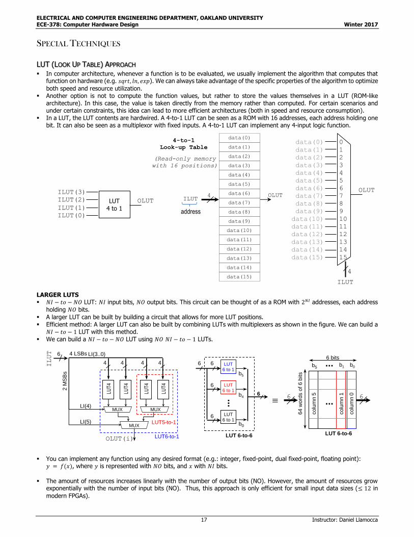
LUT (LOOK UP TABLE) APPROACH In computer architecture, whenever a function is to be evaluated, we usually implement the algorithm that computes that
function on hardware (e.g. 𝑠𝑞𝑟𝑡, 𝑙𝑛, 𝑒𝑥𝑝). We can always take advantage of the specific properties of the algorithm to optimize
both speed and resource utilization. Another option is not to compute the function values, but rather to store the values themselves in a LUT (ROM-like
architecture). In this case, the value is taken directly from the memory rather than computed. For certain scenarios and under certain constraints, this idea can lead to more efficient architectures (both in speed and resource consumption).
In a LUT, the LUT contents are hardwired. A 4-to-1 LUT can be seen as a ROM with 16 addresses, each address holding one bit. It can also be seen as a multiplexor with fixed inputs. A 4-to-1 LUT can implement any 4-input logic function.
LARGER LUTS 𝑁𝐼 − 𝑡𝑜 − 𝑁𝑂 LUT: 𝑁𝐼 input bits, 𝑁𝑂 output bits. This circuit can be thought of as a ROM with 2𝑁𝐼 addresses, each address
holding 𝑁𝑂 bits.
A larger LUT can be built by building a circuit that allows for more LUT positions. Efficient method: A larger LUT can also be built by combining LUTs with multiplexers as shown in the figure. We can build a
𝑁𝐼 − 𝑡𝑜 − 1 LUT with this method. We can build a 𝑁𝐼 − 𝑡𝑜 − 𝑁𝑂 LUT using 𝑁𝑂 𝑁𝐼 − 𝑡𝑜 − 1 LUTs.
You can implement any function using any desired format (e.g.: integer, fixed-point, dual fixed-point, floating point):
𝑦 = 𝑓(𝑥), where 𝑦 is represented with 𝑁𝑂 bits, and 𝑥 with 𝑁𝐼 bits.
The amount of resources increases linearly with the number of output bits (NO). However, the amount of resources grow
exponentially with the number of input bits (NO). Thus, this approach is only efficient for small input data sizes (≤ 12 in
modern FPGAs).
OLUT
ILUT
4
0
1
2
3
4
5
6
7
8
9
10
11
12
13
14
15
data(0)
data(1)
data(2)
data(3)
data(4)
data(5)
data(6)
data(7)
data(8)
data(9)
data(10)
data(11)
data(12)
data(13)
data(14)
data(15)
LUT4 to 1
ILUT(3)
ILUT(2)
ILUT(1)
ILUT(0)
OLUT ILUT4 OLUT
4-to-1
Look-up Table
address
(Read-only memory
with 16 positions)
data(0)
data(1)
data(2)
data(3)
data(4)
data(5)
data(6)
data(7)
data(8)
data(9)
data(10)
data(11)
data(12)
data(13)
data(14)
data(15)
6
4 4 4 4
2 M
SB
s
4 LSBs
LUT5-to-1
LUT6-to-1
LUT6 to 1
LUT6 to 1
LUT6 to 1
6
6
6
6
b0
b4
b5
b5 b1 b0
6
LUT 6-to-6
6 bits
64 w
ord
s o
f 6 b
its
LUT 6-to-6
LUT
4
LUT
4
LUT
4
LUT
4
MUX MUX
MUX
...
...
...
ILUT
LI(4)
LI(5)
LI(3..0)
colu
mn 5
colu
mn 1
colu
mn 0 66
OLUT(i)


