
i
Prediction of Travel Time and Development of Flood Inundation Maps for Flood
Warning System Including Ice Jam Scenario. A Case Study of the Grand River, Ohio
by
Niraj Lamichhane
Submitted in Partial Fulfillment of the Requirements
for the Degree of
Master of Science in Engineering
in the
Civil and Environmental Engineering Program
YOUNGSTOWN STATE UNIVERSITY
May, 2016

ii
Prediction of Travel Time and Development of Flood Inundation Maps for Flood
Warning System Including Ice Jam Scenario. A Case Study of the Grand River, Ohio
Niraj Lamichhane
I hereby release this thesis to the public. I understand that thesis will be made available from the OhioLINK ETD Center and the Maag Library Circulation Desk for public access. I also authorize the University or other individuals to make copies of this thesis as needed for scholarly research. Signature: Niraj Lamichhane, Student Date Approvals: Suresh Sharma, Thesis Advisor Date Tony Vercellino, Committee Member Date Bradley A. Shellito, Committee Member Date Dr. Salvatore A. Sanders, Dean of Graduate Studies Date
iii
ABSTRACT ...
The flood warning system can be effectively used to reduce the potential property
damages and loss of lives. Therefore, a reliable flood warning system is required for the
evacuation of people from probable inundation area in sufficient lead time. Hence, this
study was commenced to predict the travel time and generate inundation maps along the
Grand River, Ohio for various flood stages. A widely accepted hydraulic tool, Hydraulic
Engineering Center River Analysis System (HEC-RAS), was used to perform the
hydraulic simulation. HEC-GeoRAS, an ArcGIS extension tool, was used to prepare
geospatial data and generate flood inundation maps for various flood stages. A
topographic survey was conducted to obtain the accurate elevation of river channels. The
hydraulic simulations were carried out using six different elevation datasets and various
ranges of Manning’s roughness to quantify the uncertainties in travel time and inundation
area prediction due to the resolutions of the elevation datasets and Manning’s roughness.
The study showed that the coarse elevation dataset, which was 30m Digital Elevation
Model (DEM) without integration of survey data, provided higher travel time and
inundation area. It over predicted (11.03%-15.01%) in travel time and inundation area
(32.56%-44.52%) for various return period floods when compared with the results of
Light Detection and Ranging (LiDAR) integrated with survey data. Moreover, Manning’s
roughness was found to be more sensitive in channel sections than that of floodplains.
The decrease in travel time and inundation area was observed with the decrease in
manning’s roughness. The highest decrement of 21.38% and 8.97% in travel time and
inundation area was observed when roughness value was decreased in channel sections,
while the decrement in travel time and inundation area was 3.45% and 1.49% when
roughness value was decreased in floodplains. The difference in predicted travel time and
iv
inundation area, while using LiDAR integrated with survey data, was not considerably
different from 10m DEM integrated with survey data. However, LiDAR with survey data
predicted conservative travel time which would be safe to consider for the evacuation
planning from probable inundation areas. Therefore, LiDAR integrated with survey data
was used for the calculation of travel time and generation of flood inundation maps for 12
different selected flood stages. The estimated travel time can be used for the evacuation
of the people. Similarly, the rating curve and the flood inundation maps can be used to
issue flood warning. More than 100 houses, many roads, bridges and parks along the
Grand River are susceptible to 500 year return period flood. Therefore, it is suggested to
install the siren system in various locations of the river.
In addition, winter flooding due to ice jams is one of the major problems as it has
caused severe damages along the Grand River and nearby bridge structures frequently.
Therefore, the effects of ice cover and ice jams on the river level near bridges were
investigated. The increase in river stage and inundation area was observed, when ice
cover and ice jam was considered in the simulation. The average increase in river stage
was approximately 2 ft for maximum winter discharge. Likewise, the increase in
inundation area varied from 24% to 52% for various winter flows resulting in the highest
increment for the lowest winter discharge. In addition, the increase in river stage was
noticed at the upstream section of bridges during winter when the model was simulated
considering bridges. The effects of resolution of elevation datasets and ice jam/ice cover
in flood travel time and inundations maps would be valuable assets for decision makers
and planners for flood management and rescue operation in future.
v
ACKNOWLEDGEMENTS
First of all, I would like to convey my sincere thanks to my thesis advisor, Dr.
Suresh Sharma, for his continuous guidance and encouragement while conducting this
research. Also, I would like to express my sincere gratitude to thesis committee members,
Dr. Tony Vercellino and Dr. Bradley A. Shellito for their willingness to serve in my
thesis committee and provide valuable suggestions and feedbacks. Moreover, I am
thankful to the Department Chair Dr. Anwarul Islam and Dr. Peter Kimosop for their
worthful guidance and suggestions.
I would like to acknowledge for the grant support provided by Ohio Sea Grant to
conduct this research. I would also like to extend my earnest thanks to Greg Koltun of
USGS Ohio Water Science Center and Kirk Dimmick of Lake County Office, who
provided the necessary research data for this study. Also, I am much obliged to
Chrisopher R. Goodel, author of HEC-RAS User’s and Hydraulic Reference Manuals, for
providing ideas and suggestions to calibrate/validate the hydraulic model.
I am very much thankful to Linda Adovasio for her support and assistance at
YSU. I am immensely grateful to all of my friends who helped and encouraged me at
various stages during the research works and thesis writing.
Last but not the least, I am highly obliged especially to my father Hem Raj
Lamichhane and my mother Pushpa Lamichhane, who inspired and motivated me to
study and work on my thesis by taking all the family responsibilities and difficulties.
Also, I would like thank to my sisters Nisha Lamichhane and Nita Lamichhane for their
continuous support and encouragement to complete this research.
vi
Table of Contents
ABSTRACT ... ................................................................................................................ iii
ACKNOWLEDGEMENTS ................................................................................................ v
LIST OF FIGURES .......................................................................................................... vii
LIST OF TABLES .............................................................................................................. x
LIST OF ABBREVIATIONS ............................................................................................ xi
Chapter 1. Introduction ................................................................................................... 1
Chapter 2. Effect of Elevation Data Resolution and Manning’s Roughness in Travel
Time and Inundation Area Prediction for Flood Warning System .............. 8
Chapter 3. Development of a Flood Warning System and Flood Inundation Mapping
for the Grand River near the City of Painesville, Ohio .............................. 46
Chapter 4. Analysis of Winter Ice Cover and Ice Jam Effects in the Grand River Using
One Dimensional HEC-RAS Model .......................................................... 70
Chapter 5. Conclusion and Recommendations ............................................................. 94
APPENDICES .................................................................................................................. 97
vii
LIST OF FIGURES
Figure 2-1: Study area of Grand River, Ohio (Grand River watershed) ........................... 34
Figure 2-2: NLCD (2011) map of Grand River Watershed, Ohio .................................... 34
Figure 2-3: LiDAR DEM with cross section configurations of Grand River ................... 35
Figure 2-4: Hydraulic model of Grand River in HEC-RAS ............................................. 35
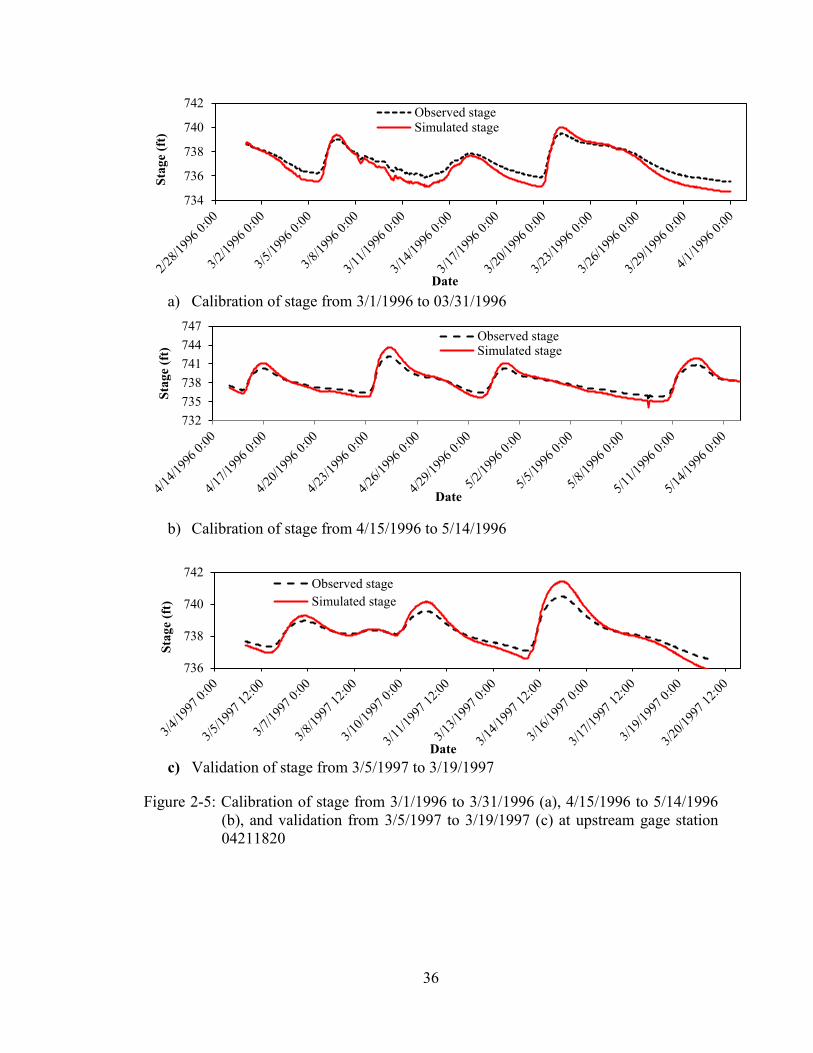
Figure 2-5: Calibration of stage from 3/1/1996 to 3/31/1996 (a), 4/15/1996 to 5/14/1996
(b), and validation from 3/5/1997 to 3/19/1997 (c) at upstream gage station
04211820 ....................................................................................................... 36
Figure 2-6: Calibration of discharge from 3/1/1996 to 3/31/1996 (a), 4/15/1996 to
5/14/1996 (b), and validation from 3/5/1997 to 3/19/1997 (c) at downstream
gage station 04212100 ................................................................................... 37
Figure 2-7: Cross section at different points along the Grand River (a)-(j) ...................... 39
Figure 2-8: Travel time and difference in travel time for different return period floods to
reach the City of Painesville using different elevation datasets1 ................... 39
Figure 2-9: Travel time and percentage difference in travel time for different return
period floods to reach Fairport Harbor using different elevation datasets1 ... 40
Figure 2-10: Inundation area and percentage difference in inundation area for different
return period floods and different elevation datasets1 ................................... 40
Figure 2-11: Difference in inundation area due to 2006 flooding in Grand River when
generated using different sets of elevation dataset ........................................ 41
Figure 2-12: Percentage decrease in inundation area for different values of Manning’s
roughness ....................................................................................................... 42
Figure 2-13: Difference in flood inundation maps for different roughness value ............ 42
viii
Figure 3-1: Historical annual peak flow/stage and various flood stage level (as per NWS)
for the ............................................................................................................. 65
Figure 3-2: Half hourly hydrograph for July 28-29, 2006 flood of Grand River, near the
City of Painesville .......................................................................................... 65
Figure 3-3: Rating curve (based on discharge greater than 75 percentile of discharge
values) for Grand River (04212100) near the City of Painesville ................. 66
Figure 3-4: Plot of predicted vs observed discharge (a), validation of the rating curve (b)
for the period of 1/1/2006 to 1/1/2015 ........................................................... 66
Figure 3-5: Travel time and flood inundation area for various flood stages at gage station
04212100 near the City of Painesville ........................................................... 67
Figure 3-6: Flood Level for the stage of 19.35 ft at gage station 04212100 at Vrooman
bridge (a), Lakeland freeway bridge (b), and Fairport road bridge (c) .......... 67
Figure 4-1: Ice jam locations in the Grand River as of CRREL Ice Jam Database, USACE
(2015) ............................................................................................................. 88
Figure 4-2: Calculated AFDD and estimated ice thickness for various winter periods.... 88
Figure 4-3: Water Surface level for various modeling scenarios near South Madison
Bridge, Madison ............................................................................................ 89
Figure 4-4: Water surface elevation for various scenarios at South Madison road (a), Blair
road (b), Vrooman road (c), Main street (d), and St. Clair street (e) along the
Grand River ................................................................................................... 90
Figure 4-5: Water surface level in Vrooman bridge for different flow conditions - cross
sectional view (a), longitudinal view (b) ....................................................... 91

ix
Figure 4-6: Inundation area and percentage increase in inundation area for various winter
flows and various simulation scenarios ......................................................... 91
x
LIST OF TABLES
Table 2-1: Datasets used in the study ............................................................................... 43
Table 2-2: Calibration/validation for stage at upstream gage station 04211820 .............. 43
Table 2-3: Calibration/validation for discharge at downstream gage station 04212100 .. 43
Table 2-4: Inundation area for different return period flood using various elevation
datasets1 ......................................................................................................... 44
Table 2-5: Decrease in inundation area when survey data is incorporated ....................... 45
Table 2-6: Travel time to City of Painesville for different Manning’s roughness values 45
Table 3-1: Discharge values for various selected stage at 04212100 based on developed
rating curve .................................................................................................... 68
Table 3-2: Comparison of high-water mark profile and modeled profile for 2006 flood. 68
Table 3-3: Summary of streamgage information in the Grand River basin, Ohio ............ 69
Table 4-1: Location, date and description of historical ice jam in the Grand River ......... 92
Table 4-2: Values for α (coefficient that accounts wind exposure and snow cover) for
different conditions taken from USACE, 2002 ............................................. 92
Table 4-3: Default values of different parameters in HEC-RAS ...................................... 92
Table 4-4: Various winter discharge values obtained from historical data ...................... 92
Table 4-5: Increase in river stage due to the presence of ice cover and ice jamming ...... 93
Table 4-6: Increase in river stage when bridge is considered in ice jam location ............ 93
xi
LIST OF ABBREVIATIONS
AFDD Accumulated Freezing Degree Days
ALERT Automated Local Evaluation in Real Time
CRREL Cold Regions Research and Engineering Laboratory
DEM Digital Elevation Model
FEMA Flood Emergency Management Agency
GIS Geographic Information System
GOES Geostationary Operational Environmental Satellite
GPS Global Positioning System
HEC-RAS Hydraulic Engineering Center River Analysis System
HUC Hydrologic Unit Code
LiDAR Light Detection and Ranging
NCDC National Climatic Data Center
NLCD National Land Cover Database
NOAA National Oceanic and Atmospheric Administration
NRCS National Resource Conservation Service
NSE Nash-Sutcliffe Efficiency
NWS National Weather Service
ODOT Ohio Department of Transportation
OGRIP Ohio Geographically Referenced Information Program
PBIAS Percent Bias
RMSE Root Mean Square Error
SFIP Standard Flood Insurance Policy

xii
TDD Thawing Degree Days
USD United States Dollars
USGS United States Geological Survey
USDA United States Department of Agriculture
USACE United States Army Corps of Engineers
USACE-HEC United States Army Corps of Engineers-Hydrologic Engineering
Center
1
Chapter 1. Introduction
Flooding is one of the most common natural disasters, which damages billions of
dollars’ worth of properties and takes the lives of many people each year (Wardsworth,
1999). Floods affect approximately 520 million people around the world, and global
economic losses due to flooding are in between 50 to 60 billion USD annually (Van et al.,
2011). In the United States alone, more than 75% of Federal disasters are associated with
flooding, which leads to an annual average death of over 80 people and properties loss of
approximately 8 billion USD (USGS, 2016). Potential losses due to flooding can be
reduced by providing reliable information to the people about the risks of flood by means
of flood warning system.
The Grand River is one of such rivers, which has flooded the City of Painesville
and nearby cities in Northeastern Ohio time and again. Having experienced extremely
wet June and July in Northeastern Ohio, the City of Painesville and adjoining cities were
flooded by the Grand River due to incessant rainfall and thunderstorms of July 27-28,
2006. Property damages of worth 30 million USD were reported due to this flood. The
United States Geological Survey (USGS) streamflow gage station at Grand River near
Painesville, Ohio recorded a highest streamflow with an estimated recurrence period of
approximately 500 years. Consequently, three counties, including Lake County of
Northeastern Ohio were declared as Federal and State disaster areas. Flooding in the City
of Painesville and the Lake Erie coastal zone was also experienced at various times of
2006, 2008 and 2011, with considerable damages and loss of the properties. Therefore,
development of a flood warning system is essential for this region.
2
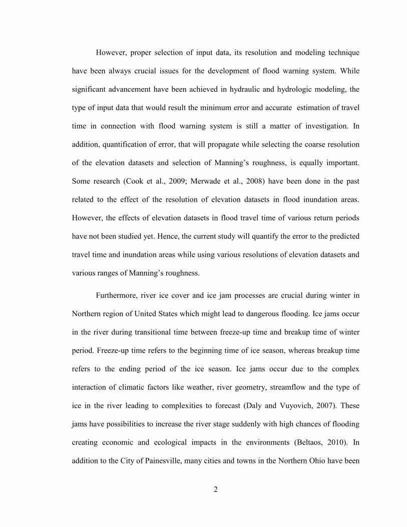
However, proper selection of input data, its resolution and modeling technique
have been always crucial issues for the development of flood warning system. While
significant advancement have been achieved in hydraulic and hydrologic modeling, the
type of input data that would result the minimum error and accurate estimation of travel
time in connection with flood warning system is still a matter of investigation. In
addition, quantification of error, that will propagate while selecting the coarse resolution
of the elevation datasets and selection of Manning’s roughness, is equally important.
Some research (Cook et al., 2009; Merwade et al., 2008) have been done in the past
related to the effect of the resolution of elevation datasets in flood inundation areas.
However, the effects of elevation datasets in flood travel time of various return periods
have not been studied yet. Hence, the current study will quantify the error to the predicted
travel time and inundation areas while using various resolutions of elevation datasets and
various ranges of Manning’s roughness.
Furthermore, river ice cover and ice jam processes are crucial during winter in
Northern region of United States which might lead to dangerous flooding. Ice jams occur
in the river during transitional time between freeze-up time and breakup time of winter
period. Freeze-up time refers to the beginning time of ice season, whereas breakup time
refers to the ending period of the ice season. Ice jams occur due to the complex
interaction of climatic factors like weather, river geometry, streamflow and the type of
ice in the river leading to complexities to forecast (Daly and Vuyovich, 2007). These
jams have possibilities to increase the river stage suddenly with high chances of flooding
creating economic and ecological impacts in the environments (Beltaos, 2010). In
addition to the City of Painesville, many cities and towns in the Northern Ohio have been
3
flooded from time to time due to extreme weather patterns associated with ice jam. Flood
prediction in this region is relatively complex because of the combined effect of ice jams
and rainfall following after snowfall. Very few studies have been conducted pertaining to
ice jam and its potential hazard using Hydraulic Engineering Center River Analysis
System (HEC-RAS) especially in the United States. More importantly, evaluation of the
impact of ice cover and ice jam flooding near hydraulic structure is essential to realize
whether the ice jams near hydraulic structures have any additional impact on flood level
or not. Therefore, development of a flood warning system, with frequently updated flood
inundation maps incorporating careful analysis of ice cover and ice jams effect, is
essential to ensure timely evacuation and reduction of the loss of lives and properties. For
this, a reliable hydraulic model should be developed using appropriate sets of input data.
A widely accepted hydraulic model HEC-RAS 4.1 was used to setup the model
and run the hydraulic simulation for the Grand River watershed in Northeastern, Ohio.
HEC-RAS model was calibrated and validated to quantify the uncertainties involved in
calculating flood travel time, generation of inundation maps and study the effects of ice
cover and ice jam in river stage and near the hydraulic structures. All these scenarios
have been described in subsequent chapters.
Scope and Objectives
Flood warning system and flood inundation maps are the necessary tools that can
be used to reduce the human and property losses. Inundation maps are useful for
preparedness before the occurrence of floods, timely response to future floods, damage
assessment, mitigation and flood risk analysis. These tools act as an important guideline
4
for decision makers, policy makers and insurance agencies to plan accordingly for future
probable flood disasters.
The main objectives of this research study are:
I. To quantify the effects of elevation data resolution and Manning’s roughness in
calculated travel time and inundation area prediction for generating reliable flood
warning system;
II. To develop an approach for flood warning system and to generate flood
inundation maps for a series of flood stages in the Grand River near the City of
Painesville, Ohio;
III. To assess the potential impact in river stage and hydraulic structures due to winter
ice cover and ice jams using one-dimensional HEC-RAS hydraulic model.
Methodology for Objective I
a. Collect input data like geospatial data, stage/discharge records, lake elevation
records required for one-dimensional HEC-RAS modeling;
b. Prepare geospatial data using six different elevation datasets in HEC-GeoRAS, an
ArcGIS extension, required for a hydraulic simulation;
c. Calibrate and validate the unsteady hydraulic model using field verified survey
and United States Geological Survey (USGS) stage/discharge records;
d. Run the simulation to calculate travel time and export the simulated data to HEC-
GeoRAS to generate flood inundation maps;
e. Compare travel time and inundation maps for various elevation datasets to
quantify the effects of elevation data resolution and Manning’s roughness.

5
Methodology for Objective II
a. Prepare flood discharges data for various flood stages (at streamgage 04212100,
near the City of Painesville) as an input for steady hydraulic model;
b. Calibrate/validate for steady flow scenario using high-water marks of 2006 flood;
c. Run the simulation for 12 different flood stages to predict travel time and generate
probable flood inundation maps as a part of the flood warning system.
Methodology for Objective III
a. Collect historical temperature, precipitation and ice jam location information and
estimate ice thickness using modified Stefan’s equation;
b. Prepare input data including winter discharge records and ice thickness
information to simulate model;
c. Run the simulation for various scenarios including/excluding ice cover/ice jams
and bridges;
d. Compare and analyze these scenarios and evaluate the difference in river stages for
different scenarios.
Thesis Structure
This thesis is mainly divided into four chapters. Chapter 1 describes background,
scope, objectives and thesis structure. Chapter 2 quantifies the error propagated with
elevation data resolution and Manning’s roughness values in channel and floodplains for
the computation of flood travel time and inundation area. This chapter also gives the
detail description of theoretical background, overall modeling approach, model input data
and calibration/validation procedure of one-dimensional unsteady flow HEC-RAS model,
which is crucial for further study.
6
Chapter 3 discusses the calculation of flood travel time and generation of flood
inundation maps for various stages of floods along the Grand River. Additionally, it
discusses an approach for the development of flood warning system. The same calibrated
and validated unsteady flow model as discussed in Chapter 2 was used for this analysis.
In addition, it further discusses the calibration of the model in steady flow using high-
water marks of 2006 flood along the Grand River, near the City of Painesville as a part of
the flood warning system development.
Chapter 4 discusses the effects of winter ice cover and ice jam in the flood level
and inundation area along the Grand River. Additionally, the effects of ice cover and ice
jam in hydraulic structures like bridge locations have been discussed. A comparative
study has been done to see the differences in flood level and inundation area when ice
jam occurs in the winter season in the Grand River.
In Chapter 5, the conclusions derived from this study and the recommendations
for future work to develop more effective and automated flood warning system have been
discussed.
Chapter 2 and Chapter 4 have been structured in journal paper format. These
chapters will be developed as a full-length article after some additional work in the
future. Since journal article should stand alone with sufficient background information,
the readers may find some redundancies in these chapters.
7
References
Beltaos, Spyros. "Assessing Ice-Jam Flood Risk: Methodology and Limitations." 20th
IAHR Inernational Symposium on Ice. 2010.
Cook, Aaron, and Venkatesh Merwade. "Effect of topographic data, geometric
configuration and modeling approach on flood inundation mapping." Journal of
Hydrology 377.1 (2009): 131-142.
Daly, Steven F. and Vuyovich, Carrie. “Ice Jam Formation Parameters in Selected U.S.
Rivers” USACE, 2007
King, Rawle O. "National flood insurance program: Background, challenges, and
financial status." Congressional Research Service, Library of Congress, 2009.
Merwade, Venkatesh, et al. "Uncertainty in flood inundation mapping: current issues and
future directions." Journal of Hydrologic Engineering13.7 (2008): 608-620.
NOAA, 1981. Floods, Flash Floods and Warnings, Pamphlet, National Weather Service,
NOAA, Washington, DC.
Sangwan, Nikhil. Floodplain mapping using soil survey geographic (SSURGO) database.
Diss. PURDUE UNIVERSITY, 2014.
USGS, 2016. USGS Flood Inundation Mapping Science, Flood Inundation Mapping
(FIM) Program (accessed March 2016) http://water.usgs.gov/osw/flood_
inundation/
Van Alphen, J., et al. Flood risk management approaches: As being practiced in Japan,
Netherlands, United Kingdom and United States. IWR, 2011.
Wadsworth, G. 1999. Flood Damage Statistics. Public Works Department, Napa, CA.
8
Chapter 2. Effect of Elevation Data Resolution and Manning’s Roughness in Travel Time and Inundation Area Prediction for Flood Warning
System
Abstract
The flood travel time and possible area of inundation are two crucial issues in
flood warning system to allow timely evacuation of people in sufficient lead time from
the probable inundation area. Therefore, accurate travel time computation and floodplain
mappings are essential to develop a flood warning system. While earlier research were
more focused on the uncertainty of data resolution in floodplain mapping, the major
objective of this study was to compute travel time for the timely evacuation and generate
various return period floodplain maps, within the range of uncertainties associated with
various resolutions of datasets and Manning’s roughness. This was accomplished using
one-dimensional hydraulic model, Hydraulic Engineering Center River Analysis System
(HEC-RAS). Geospatial data required for HEC-RAS was obtained using various
resolution Digital Elevation Model (DEM) datasets, which was pre-processed in HEC-
GeoRAS. The hydraulic analysis was performed in HEC-RAS and post-processed in
HEC-GeoRAS to produce flood inundation maps. The travel time and flood maps were
analyzed using various Manning’s roughness values with six elevation datasets: Light
Detection and Ranging (LiDAR) data; 10m DEM; 30m DEM; integration of survey data
with LiDAR data; integration of survey data with 10m DEM; and integration of survey
data with 30m DEM. It was found that travel time and inundation area could be
overestimated if coarser elevation datasets were used. The maximum difference in
calculated travel time was 11.03%-15.01% and in predicted inundation area was 32.56%-
44.52% for 30m DEM without integration of survey data. This error was based on the
comparison of the result obtained with Light Detection and Ranging (LiDAR) data
9
modified with field verified survey data. The minimum difference in calculated travel
time was 0.50%-4.33%, and predicted inundation area was 3.55%-7.16% while using
10m DEM along with survey data. The difference in travel time and possible inundation
area generated from LiDAR with survey data was not significantly different from 10m
DEM with survey data. However, LiDAR with survey data provided a conservative
prediction in travel time which would be safe to plan for evacuation from possible flood
prone areas. While 10 m DEM best represented the actual field survey section in channel
compared to LiDAR data, the application of LiDAR data was pertinent as flood usually
travels through the floodplain especially during high flow period and also provides
elevation at high resolution. Since the topographical study was done for this study,
LiDAR data with field verified cross sections were used to calculate flood travel time and
generate inundation maps. Additionally, Manning’s roughness of channel section was
found to be more sensitive than that of floodplains while computing travel time and
generating inundation maps. The decrease in inundation area was the highest (8.97%)
while using the lower value of Manning’s roughness (0.020).
Keywords: Floodplain mapping, Topographic dataset, River bathymetry, HEC-RAS,
HEC-GeoRAS,
Introduction
Flooding is one of the most common forms of natural calamities in many
countries across the world, which may damage millions of dollars’ worth properties and
may take the lives of thousands of people every year (Basha et al., 2007; King 2010;
Lowe 2003). Flood caused more human lives and property losses (90% of all property
losses) than any other forms of natural calamities in the twentieth century in the United
States (Krimm 1996; Perry 2000). One of the ways to prevent from such calamities and
10
losses is to develop flood warning system and inform the people in the community for the
evacuation in sufficient lead time. Therefore, the determination of flood travel
(evacuation) time is essential for the timely evacuation of people from probable
inundation area and to minimize the negative consequences of such hazards
(Krzysztofowicz et al., 1994). On the other hand, it is equally important to make these
floodplain maps easily accessible and comprehensible to the public without difficulties
(Holtzclaw et al., 2005). Floodplain maps are very important tools, which represent the
spatial variability of flood hazards and provide the direct and robust understanding of
floods than any other forms (Merz et al., 2007; Leedal et al., 2010). While there has been
a significant advancement in hydrologic and hydraulic models to generate floodplain
maps, uncertainties associated with topography, vegetation/topography characteristics,
flow discharge, techniques and methods of modeling still exist in floodplain mapping
process (Marks and Bates, 2000; Crosetto et al., 2001; Smemoe et al., 2003; Merwade et
al., 2008; Bales et al., 2009). Since the floodplain mapping process is not an exact science
(Smemoe et al., 2003), probabilistic floodplain maps generated considering uncertainties
in modeling are appropriate rather than deterministic maps while planning for the future
rescue operation and quantification of flood insurance rates in probable affected areas (Di
Baldassarre, 2012).
Some research has been previously conducted to study the uncertainties
associated with flood inundation mapping process. Merwade et al. (2008) conducted a
study in Strouds Creek, North Carolina in floodplain mapping and reported the
uncertainties due to hydrologic flow including the complex interaction of individual
inputs in hydraulic model. Similarly, another study was conducted in Strouds Creek in
North Carolina and Brazos River in Texas (Cook and Merwade, 2009) to study the
11
effects of topographic data and the geometric configuration in flood inundation maps.
The study concluded that the predicted area decreases with higher resolution of
topographic data. Various other studies (Horrit & Bates, 2001; Bates et al., 2004;
Domeneghetti et al., 2013; Dottoti et al., 2013) have been conducted to comprehend the
uncertainties in flood inundation maps. However, to the best of my knowledge, no study
has been conducted yet to quantify the potential uncertainties in flood travel time of
various return periods when different elevation datasets and Manning’s roughness values
are used.
Therefore, the major objective of this research is to calculate the flood travel time
and generate floodplain maps corresponding to different return period floods in the City
of Painesville located along the Grand River of Lake County, Ohio. The uncertainties
associated with flood travel time and the extent of flood inundation maps while using
various resolutions of elevation datasets and different values of Manning’s roughness are
also reported. For this, the HEC-RAS model was developed for flood magnitude of
different return period. Finally, the effects of elevation data resolutions and Manning’s
roughness have been reported for the appropriate representation of flood travel time and
the flood extents.
Theoretical Description
The hydraulic modeling software, HEC-RAS, was used in this study for steady
and unsteady flow analysis. HEC-RAS was developed by United States Army Corps of
Engineers-Hydrologic Engineering Center (USACE-HEC), which has been widely used
for steady flow analysis, unsteady flow simulation, movable boundary sediment transport
computations and water quality analysis (Brunner, 1995). Usually, steady flow approach
12
is used for floodplain management and flood insurance studies, whereas unsteady flow
approach is used for subcritical flow regime especially for dam break analysis and
pressurized flow module (Brunner, 1995; Brunner, 2002). The effect of various
obstructions such as culverts, bridges, dams and weirs can be considered in the analysis
to see their impacts in the water surface profiles. HEC-RAS solves one-dimensional,
Saint-Venant equations, using four-point implicit method developed for natural channels
(Brunner, 2002) to simulate unsteady flow, which are derived from the continuity and
momentum equations. The continuity and momentum equations have been listed as
follows.
𝜕𝐴
𝜕𝑡+
𝜕𝑄
𝜕𝑥= 0 (2.1)
𝜕𝑄
𝜕𝑡+
𝜕(𝑄2
𝐴)
𝜕𝑥+ 𝑔𝐴
𝜕𝐻
𝜕𝑥+ 𝑔𝐴(𝑆0 − 𝑆𝑓) = 0 (2.2)
Where A is cross-sectional area normal to the flow; t is any time; Q is discharge of
river; x is longitudinal distance in the river; g is acceleration due to gravity; H is elevation
of water surface in the river above assumed datum level; S0 is slope of river bed, and Sf is
energy slope of water.
The Saint-Venant equations are solved using the well-known four point implicit
finite difference scheme in HEC-RAS. This scheme is completely non-destructive but
marginally stable (Fread 1974; Ligget and Cunge, 1975) when it is run in semi-implicit
form (weighting factor θ of 0.5). The value of θ in HEC-RAS varies from 0.6 to 1. The
value of 1 provides the most stable form, whereas a value of 0.6 provides the greatest
stability of the solution (Brunner, 2002).
13
In steady flow simulation, HEC-RAS solves energy equation as given below to
calculate water surface elevations from one cross section to another cross section with an
iterative procedure which is called as standard step method (Brunner, 1995).
𝑍1 + 𝑌1 +𝑎1𝑉1
2
2𝑔+ 𝐻𝑒 = 𝑍2 + 𝑌2 +
𝑎2𝑉22
2𝑔 (2.3)
Where Z1 and Z2 are elevations of the main channel, Y1 and Y2 are depths of water, V1 and
V2 are average velocities, and α1 and α2 are velocity weighting coefficients at section one
and two respectively. Similarly, g is acceleration due to gravity, and He is energy head
loss from section one to section two.
Materials and Methodology
Study Area
This study was conducted in the Grand River watershed, which consists of major
three tributaries: Mill, Paine and Big Creek. The watershed which is located in
Northeastern region of Ohio and has an area of 705 mi2 with an elevation range from a
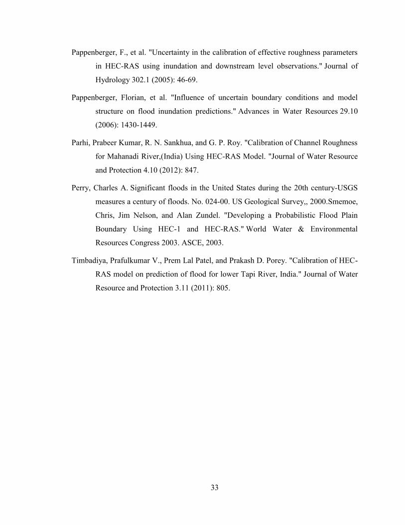
minimum of 564 ft to maximum of 1385 ft (Figure 2-1). It has twenty-eight Hydrologic
Unit Code (HUC)-14 watersheds and six HUC-11 watersheds, which spread out to five
counties; Lake, Ashtabula, Trumbull, Geauga and Portage. The watershed is
geographically surrounded within N 41̊ 22’ to N 41̊ 51’, E -80̊ 35’ to E -81̊ 18’. The
Grand River originates from the southern part of Middlefield and flows through Orwell,
Rock Creek, Austinburg, Harpersfield, Madison, Perry, Painesville, Fairport Harbor and
finally ends to the Lake Erie. The river is approximately 102.7 miles with an average
slope of 1 in 900 and an average width of approximately 275 ft., varying from 150 ft to
500 ft at various locations. The mean annual precipitation in the watershed is found to be
38 inches based on the historical records. In this study, a river section of approximately
14
32.2 miles from Harpersfield to Fairport Harbor, which includes the City of Painesville,
was considered as a study site to perform the hydraulic analysis.
The City of Painesville along the Grand River has been frequently threatened by
several flooding that occurred from time to time (2006, 2008, and 2011). The disastrous
flood of July 27-28, 2006 in Grand River caused by more than 11 inches of rainfall depth,
led to the destruction of 100 homes and business, five bridges and 13 roads. Property
worth of 30 million USD was damaged including one death in Lake County.
Consequently, hundreds of people were evacuated and three counties including Lake,
Geauga and Ashtabula were declared as Federal and State disaster areas (Ebner et al.,
2007). This flood was reported to have a peak flow of 35,000 cfs (500 return year period)
and highest historic stage of 19.35 ft (Ebner et al., 2007) as recorded by USGS gage
station (04212100) near the City of Painesville.
Overall Modeling Approach
In order to calculate accurate flood travel time and generate floodplain maps,
calibrated and validated one-dimensional hydraulic model, HEC-RAS, was developed by
importing the geospatial data of river cross sections and bridges from HEC-GeoRAS. The
HEC-GeoRAS is a tool that uses graphical user interface for preparing geospatial data in
ArcGIS. Unsteady flow simulation for different flood events for the period of 1996-1998
was performed for model calibration and validation. Since steady flow simulation is
typically performed during peak flood period (Hicks et al., 2005; Cook, A.C. 2008), peak
flood was simulated in steady flow conditions to calculate the flood travel time and water
surface elevations. These water surface elevations/extents were then exported back to
HEC-GeoRAS to produce floodplain maps. Typically, elevation datasets such as National
Elevation Datasets (NED) and Light Detection and Ranging (LiDAR) do not include the
15
river bathymetry leading to the requirement of field verification through the
topographical survey. Therefore, the river was surveyed using highly accurate Global
Positioning System (GPS) technology from Harpersfield to North St. Clair Bridge. For
the remaining portion up to Lake Erie near Fairport Harbor, bathymetry survey using
sounding method produced by National Oceanic and Atmospheric Administration
(NOAA) and USACE was used. Six different topographical datasets including LiDAR
derived DEM, 10m DEM, 30m DEM, and integration of field verified cross section with
each datasets of LiDAR derived DEM, 10m DEM and 30m DEM were used in this study.
The differences in the travel time and floodplain extents were compared and reported
using such various resolution datasets.
HEC-GeoRAS/HEC-RAS Model Input
Elevation data sets are needed to generate geospatial data and perform hydraulic
analysis in HEC-RAS. Therefore, high-quality datasets were used in this study in order to
compute travel time and produce accurate flood inundation maps. LiDAR data was
downloaded from Ohio Geographically Referenced Information Program (OGRIP)
website. Similarly, Digital Elevation Model (DEM) of 10 m and 30 m resolutions were
downloaded from National Resource Conservation Service-United States Department of
Agriculture (NRCS-USDA), Geospatial Data Gateway. Land use data of 30 m resolution
was downloaded from National Land Cover Database 2011 (NLCD 2011). The Grand
River watershed includes forest (41.86%), cultivated land (24.57 %), waterbodies and
wetlands (7.67%) and developed/urban land (10.21%). The remaining 15.70% are
covered by other land such as Herbaceous (4.2%), barren land (0.08%), hay/pasture
(9.29%) and shrub/scrub (2.13%) as per NLCD 2011 (Figure 2-2).
16
Geometric input features classes needed for HEC-RAS such as stream lines, cross
sections, bank stations, storage areas were first created in HEC-GeoRAS and then
exported to HEC-RAS. In order to represent the accurate cross section of the river, the
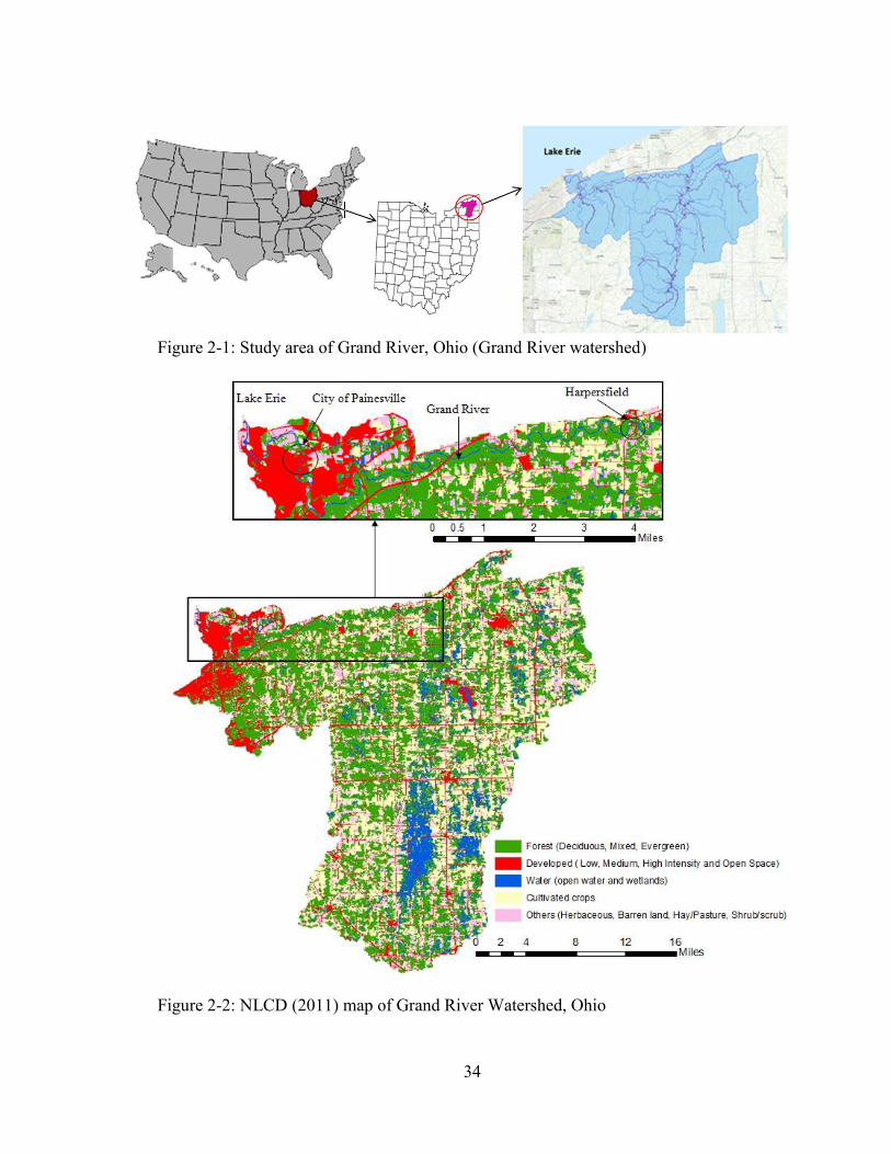
topographical survey was performed at 77 different sections of the river (Figure 2-3). The
cross sections were surveyed at an interval of half a mile to a mile depending upon the
site conditions. The hydraulic model, HEC-RAS, developed for Grand River after
incorporating river cross section is shown in Figure 2-4. Discharge and stage data for the
station 04211820 (upstream gage station near Harpersfield) and 04212100 (downstream
gage station near the City of Painesville) were obtained from USGS website to perform
unsteady hydraulic analysis and calibrate Manning’s roughness for study reaches in
HEC-RAS. Peak discharge data for the recurrence interval of 10, 50, 100, and 500 years
for Grand River were obtained from Koltun et al. (1990), which was determined based on
log-Pearson Type III distribution. For other ungauged stream reaches including Mill,
Paine and Big Creek, peak discharge from 10 to 500 years return periods were obtained
from streamstat web application (Guthrie et al., 2008). The streamstat calculates the peak
discharge based on different regression equations (Koltun et al., 1990) depending upon
the river basin characteristics. There are altogether 10 bridges within the study area, and
the data for these bridges were obtained from Lake County Office and Ohio Department
of Transportation (ODOT). Similarly, the data for high flood levels for Lake Erie has
been obtained from a report by USACE (USACE 2000). The summary of input data
including their types and sources are presented in Table 2-1.
Model Calibration and Validation
The unsteady HEC-RAS model was calibrated by the iterative process to obtain
the suitable value of Manning’s roughness for river reaches by comparing simulated stage
17
and discharge with the observed data. The preliminary selection criteria of Manning’s
roughness has been recommended by various approaches including visual inspection,
land use/land cover and optimization techniques rather than selecting it only from
intuition approach (Kalyanapy et al., 2010). Channel roughness is highly variable as it
depends on many factors like channel alignment, surface roughness, bed material, nature
of sediments and obstruction present in the channel (Pappenberger et al., 2005;
Timbadiya et al., 2011; Parhi et al., 2012). Chow et al. (1988) illustrates that the
Manning’s roughness varies from 0.035 to 0.065 for the main channel and 0.08 to 0.15 in
the floodplains. Regardless, it needs to be calibrated using the known years flood data;
therefore, eight different minor and major flood events from 1996-1998 were used in
HEC-RAS simulation. Finally, the calibrated Manning’s roughness values were used to
calculate travel time and develop the flood inundation maps.
Model Evaluation Criteria
Various statistical parameters such as Nash-Sutcliffe efficiency (NSE), R-squared
(R2), percent bias (PBIAS) and root mean square error (RMSE) were used to test the
accuracy and predictive power of the model (ASCE 1993; Gupta et al., 1999; Moriasi et
al., 2007).
The NSE is a standardized statistic criteria that determines the relative magnitude
of the residual variance ("noise") compared to the variance of measured data (Nash and
Sutcliffe, 1970). NSE is recommended for model evaluation as it is found to be the best
objective function for reflecting the overall fit of a hydrograph (Moriasi et al., 2007).
Typically, it indicates the wellness of observed and simulated data fitting the 1:1 line. Its
value ranges from -∞ to 1, and values from 0 to 1 are acceptable. The NSE value of 1 is
18
rare and considered as a perfect value for an ideal model. NSE is calculated by using the
following equation.
𝑁𝑆𝐸 = 1 − [∑ (𝑌𝑖
𝑜𝑏𝑠−𝑌𝑖𝑠𝑖𝑚)
𝑛
𝑖=1
2
∑ (𝑌𝑖𝑜𝑏𝑠−𝑌𝑜𝑏𝑠
𝑚𝑒𝑎𝑛)𝑛
𝑖=1
2] (2.4)
Where 𝑌𝑖𝑜𝑏𝑠 is the ith value of observed data, 𝑌𝑖
𝑠𝑖𝑚 is the ith value of simulated
data, 𝑌𝑜𝑏𝑠𝑚𝑒𝑎𝑛 is the mean value of observed data, 𝑌𝑠𝑖𝑚
𝑚𝑒𝑎𝑛 is the mean of simulated data, and
n is the total number of observations.
R2 measures the fitness of observed and simulated data. R2 varies from 0 to 1,
indicating 1 as a perfect fitness of data.
𝑅2 = (∑ (𝑌𝑖
𝑜𝑏𝑠−𝑌𝑜𝑏𝑠𝑚𝑒𝑎𝑛)(𝑌𝑖
𝑠𝑖𝑚−𝑌𝑠𝑖𝑚𝑚𝑒𝑎𝑛)
𝑛
𝑖=1
[∑ (𝑌𝑖𝑜𝑏𝑠−𝑌𝑜𝑏𝑠
𝑚𝑒𝑎𝑛)2𝑛
𝑖=1∑ (𝑌𝑖
𝑠𝑖𝑚−𝑌𝑠𝑖𝑚𝑚𝑒𝑎𝑛)
2𝑛
𝑖=1]
0.5)
2
(2.5)
RSR is the ratio of RMSE and standard deviation of the observed data. Lower the
value of RSR, lower is the root mean square error and better is the model performance.
The ideal value of RSR is 0. The RSR is calculated by using following equation.
𝑅𝑆𝑅 =𝑅𝑀𝑆𝐸
𝑆𝑇𝐷𝐸𝑉𝑜𝑏𝑠=
√∑ (𝑌𝑖𝑜𝑏𝑠−𝑌𝑖
𝑠𝑖𝑚)2𝑛
𝑖=1
√∑ (𝑌𝑖𝑜𝑏𝑠−𝑌𝑜𝑏𝑠
𝑚𝑒𝑎𝑛)2𝑛
𝑖=1
(2.6)
PBIAS is the percentage deviation in simulated data from the observed data
(Moriasi et al., 2007). PBIAS with value 0 is considered as a perfect model harmonizing
with the observed data. Negative values of PBIAS specify overestimation bias, whereas
positive values of PBIAS indicate underestimation bias. PBIAS is calculated using
following equation.
𝑃𝐵𝐼𝐴𝑆 = [∑ (𝑌𝑖
𝑜𝑏𝑠−𝑌𝑖𝑠𝑖𝑚)
𝑛
𝑖=1𝑋 100
∑ (𝑌𝑖𝑜𝑏𝑠)
𝑛
𝑖=1
] (2.7)
19
Uncertainties Associated with Floodplain Modeling
A large number of uncertainties accompanied with numerous variables including
topography, Manning’s roughness, flow discharge, techniques and methods of modeling
are still associated with the floodplain mapping regardless the advancement in hydrologic
and hydraulic modeling tools (Oegema and McBean, 1987; Merwade et al., 2008;
Smemoe et al., 2003). Therefore, the accuracy of the floodplain maps depends on how
these uncertain variables have been incorporated in hydraulic and hydrologic models
(Merwade et al., 2008). Two important variables, which may impose errors in flood
travel time and inundation area, have been discussed in this study.
Effect of Topography
The reliable elevation datasets are essential for the generation of accurate flood
inundation maps. The use of high-resolution LiDAR data, somehow, might improve the
accuracy of floodplain mapping as it provides highly accurate elevation data. However, it
does not represent the exact river bathymetry, which may still pose serious errors in
travel time calculation and flood inundation mapping. According to Merwade et al.
(2008), the poor quality of terrain data can impose error in flood inundation mapping
process in three ways. Firstly, it affects the streamflow generated from hydrological
models. Secondly, it affects the river stage calculated from hydraulic models, and lastly,
it affects the spatial extents of floods. So, the field verified cross sections of river reaches
are absolutely essential to get the better bathymetry of the river for travel time
computation and floodplain mapping.
Effect of Manning’s Roughness
Since the complete characteristics of terrain are reflected by Manning’s
roughness, it plays a significant role in model calibration and floodplain delineation. The
20
roughness value varies spatially along the river depending upon the river bed material
and surrounding floodplain characteristics. It is essential to adequately represent the
roughness characteristics of the floodplain and channel in order to reduce the
uncertainties involved in the flood travel time and floodplain mappings. The preliminary
selection of Manning’s roughness was based on the terrain properties of other similar
rivers as presented in Arcement et al. (1989) and Barnes, (1849). The hydraulic model in
this study was simulated for different values of channel roughness to study the
uncertainties associated with it.
Effect of Discharge
River discharge is also considered as one of the uncertain variables that has to be
considered in floodplain mapping (Oefema & McBean, 1987; Pappenberger et al., 2006b;
Merwade et al., 2008; Di Baldassarre & Montanari, 2009). The discharge values for
various return period floods were generated from the regression equation derived by
USGS (Koltun et al., 1990). Error associated with discharge prediction for tributaries can
be dissipated in water surface elevation and the flood extents calculated from hydraulic
model (Merwade et al., 2008).
Results and Discussions
Simulation of Hydraulic Model
The performance of the model was good in calibration and validation based on the
evaluation measured through different statistical criteria. The calculated value of all
statistical parameters was higher than the recommended values (NSE > 0.50, PBIAS
±25% and RSR ≤ 0.70) by Moriasi et al. (2007). The detail results of
calibration/validation for the stage at upstream gage station 04211820 are presented in
Table 2-2. Similarly, the detail results of calibration/validation for discharge at
21
downstream gage station 04212100 are presented in Table 2-3. In this study, NSE for
stage calibration/validation varied from 0.74 to 0.89 (Table 2-2), and NSE for discharge
calibration/validation varied from 0.69 to 0.96 (Table 2-3) except for a period 2/26/1997
to 3/3/1997.
Furthermore, the performance of the model was also evaluated through the visual
inspection using the graphical plot of observed and simulated stage/discharge. The
calibration/validation of stage at upstream gage station 04211820 is shown in Figure 2-5.
Similarly, the calibration/validation of discharge at downstream gage station 04212100 is
shown in Figure 2-6. The model efficiency was assessed for several possible values of
Manning’s roughness, and the roughness value was calibrated based on the performance
efficiency of simulated result with observed data. Overall, the model performance was
well above the satisfactory range. The calibrated/validated value of Manning’s roughness
was adopted 0.035 for channels and 0.15 for banks/floodplain regions.
Effect of Topography
The effect of topography on flood inundation extents depends on the size of the
river, bathymetry of the river, and the hydraulic modeling approach (Merwade et al.,
2008). The elevation of rivers at different cross sections greatly varied when different sets
of elevation datasets were used. The cross sections for 10 different locations generated
from 4 different elevation datasets are shown in Figure 2-7. It was found that, in majority
of those cross sections, the topographic data represented by 10 m DEM was better than
LiDAR data particularly in channel sections indicating that cross section generated from
10m DEM was better representing to the actual cross sections. This is not surprising as
airborne LiDAR cannot penetrate water (Allouis et al., 2007) especially in the channel
22
sections. However, LiDAR data are expected to represent the floodplain well, as these
data are prepared in high resolution.
The study found out that the travel time of different return period floods varied
based on the resolution of the datasets that were used in the hydraulic analysis. Travel
time to reach the City of Painesville and Fairport Harbor for five different return period
floods was calculated using six different elevation datasets. The graphical representation
of travel time and percentage difference in travel time for various year return period
floods to reach the City of Painesville is shown in Figure 2-8. The calculated travel time
was found to be the highest for the most coarse elevation dataset (30m DEM without
survey) and was on decreasing order for finer elevation datasets with an exception for
LiDAR data. For example, the difference in calculated travel time for various return
period floods was maximum (11.03% to 15.01%) for 30m DEM without integration of
survey data and minimum (1.19%-3.35%) for 10m DEM while integrated with survey
data. It was interesting to mention that 10 m DEM without integrating the survey data
revealed small difference in travel time to the City of Painesville when compared to the
travel time computed using LiDAR data without survey. The percentage difference for
10m DEM without survey was 3.67%-4.87%, whereas it was 10.24%-11.75% for LiDAR
without survey. A similar pattern was detected for the case of travel time from
Harpersfield to Fairport Harbor. The graphical representation of travel time and
percentage error in travel time for different return period floods to reach Fairport Harbor
is shown in Figure 2-9. There was the maximum difference of 13.29%-14.28% in
calculated travel time for 30 m DEM without integration of survey data for various return
period floods. However, the minimum difference of 0.50%-4.33% was detected for 10m
DEM integrated with survey data (Figure 2-9). The calculated travel time for LiDAR data
23
without integration of survey data was relatively higher. One of the reasons for this could
be due to the coarser elevation data in channel sections as airborne LiDAR data cannot
penetrate water bodies to accurately portray the river bed elevation. Similarly, the water
surface elevation and total flow area for LiDAR data without integration of survey data
were also found to be higher than some other coarser elevation datasets. Consequently,
the flow and computed velocity was relatively smaller resulting to higher travel time.
Therefore, bathymetric data is absolutely needed for the appropriate representation of
river profile. Since bathymetric LiDAR data were not available, the detail survey was
conducted along the channel sections to modify the cross section and best represent the
site conditions in the model. The river cross sections after detailed survey were
incorporated in the LiDAR data in channel sections. This decreased the travel time to
reach the City of Painesville by 10.24 % to 11.75% (Figure 2-8) and by 2.33% to 6.84%
to reach Fairport Harbor for various return period floods (Figure 2-9).
Furthermore, inundation maps were also generated for five different return period
floods using six elevation datasets. The graphical representation of inundation area
including its percentage difference for different return period floods and different
elevation datasets are shown in Figure 2-10. Similarly, the tabular details of inundation
area for each return period floods calculated using various elevation datasets and the
percentage difference are shown in Table 2-4. It was found that the inundation area
increased with the coarser resolutions of elevation datasets. For example, the inundation
area for 500 return year period flood using LiDAR data with survey was 4.10 mi2 and
using 30 m DEM without survey was 5.55 mi2 with an area difference of 35.37%. The
maximum difference in inundation was found to be 32.56%-44.52% for 30 m DEM
without integration of survey data for various return period floods and the minimum
24
difference was 3.55%-7.80% for 10 m DEM while integrated with survey data (Table
2-4). The flood maps of 2006 flood period were generated using various elevation
datasets to have a clear picture of inundation area difference. These flood maps were
generated in HEC-GeoRAS and are shown in Figure 2-11. The importance of detail
bathymetry data to generate inundation maps was clearly observed. When the bathymetry
data (survey data) was incorporated in DEM, the decrease in predicted inundation area
was observed. The average reduction in inundation area of five different return period
floods was found to be the highest (17%) for 30m DEM and least (9%) for LiDAR (Table
2-5). This finding was consistent with the result presented by Merwade et al. (2008).
Also, we compared the top width and the flow area for 2006 flood at several
locations of the river. In most of the cases, there was a decrement in top width and flow
area after the integration of bathymetry data. The decrement percentage was higher for
30m DEM and least for LiDAR data. Moreover, there was an increase in channel velocity
and total average velocity which resulted decreasing the travel time for various return
period floods when survey data was incorporated.
Effect of Manning’s Roughness
As stated earlier, the result showed the difference in travel time and inundation
maps when series of different Manning’s roughness values were used. In this study, five
different return period floods in Grand River were analyzed in two different ways. First,
we considered the constant value of roughness in the channel section while varying the
roughness value in floodplains. Four different roughness values (0.15, 0.10, 0.09 and
0.07) within acceptable range were chosen to see the variation. The detail results of travel
time to the City of Painesville for different values of Manning’s roughness are presented
in Table 2-6. The lower values of Manning’s roughness in floodplains resulted in the
25
increased travel time even though the increment was not significant. The maximum
increment was found to be 3.45% for 2006 flood when the roughness value was the
lowest (0.07) among those four different values (Table 2-6). Secondly, a constant value
of roughness was considered in floodplains and varied in channel sections. For this, four
different possible roughness values (0.035, 0.030, 0.025, and 0.020) in channel were
chosen. As the roughness value was lowered in channel section, there was significant
decrease in travel time for different return period floods. The maximum decrement
ranged from 20.72%-22.35% when roughness value was 0.020 at channel section (Table
2-6). The main reason for the decrement was an increase in channel flow velocity due to
a decrease in roughness value.
Similarly, the effect of Manning’s roughness was observed in inundation area as
well. Floodplain maps were produced for different sets of roughness values in channel
and floodplain regions. There was a decrease in flood inundation area for lower values of
Manning’s roughness than that of the calibrated/validated values. The percentage
decrease in inundation area while using different values of Manning’s roughness is
shown in Figure 2-12. In the first case (roughness value was lowered in floodplain region
but kept constant in channel), the percentage decrease in inundation area was less than
1.49 %. However, in the second case, (roughness value was lowered in the channel but
kept constant in floodplains), the percentage decrease in inundation area was 8.97%
(Figure 2-12). The sensitivity of roughness in floodplain mapping is found to be higher in
the second case. The decrease in inundation area was noticed mostly in the flat regions
along the river. Therefore, the appropriate calibration of Manning’s roughness at channel
sections is more crucial. The difference in predicted inundation area for different
Manning’s roughness is shown in Figure 2-13.
26
Conclusion
Accurate floodplain maps are essential tools for floodplain managers and
insurance actuaries to make appropriate decisions to plan for rescue operation in affected
areas during flooding periods. In this paper, the effects of the resolution of topographic
datasets and Manning’s roughness value in the prediction of flood travel time and
inundation areas have been discussed. Five different return period floods including 10,
50, 100, 500 years and 2006 flood were considered for analysis. These different floods
were simulated in a widely recognized hydraulic tool, HEC-RAS, using various
topographic datasets wide ranges of Manning’s roughness. A topographic survey was
carried out to represent accurate elevation dataset in the river channel sections assuming
that LiDAR data gives the correct elevation representation especially in floodplains. The
surveyed elevation datasets were integrated with high-resolution LiDAR data.. Among all
elevation datasets, the travel time was highest for the coarse data (30m DEM without
integration of survey data) and had a decreasing trend for high resolution data. However,
the calculated travel time obtained from 10m DEM without integration of survey data
showed less difference than the result obtained from LiDAR without integration of
survey. Therefore, it can be concluded that the elevation data in channel section is better
represented by 10m DEM than LiDAR in case field survey data are not available.
However, the predicted inundation area from LiDAR without survey had less area
difference than that of 10m DEM without survey. Nevertheless, a topographic survey is
required to get the actual representation of the land surfaces in channel sections.
In this study, LiDAR with the integration of survey data gave conservative travel
time. Since, it is always safe to make a decision based on the worst case scenario, lesser
travel time would be appropriate for evacuation planning from the possible inundation
27
areas. Similarly, the predicted area of inundation also increased as the coarser resolution
of datasets was used, and the percentage difference was very high for 30m DEM without
integration of survey. Therefore, it can be concluded that very coarse dataset considered
in this study (30m DEM without integration of survey data) is not appropriate for the
calculation of travel time and the generation of flood inundation maps. The differences in
results were significant in 30m DEM even after the integration of survey. It was also
found that there was a decrement in travel time, inundation area, flow area and top width
and increment in the flow velocity when the bathymetry data was integrated to any
resolution of dataset. Therefore, when coarse datasets are used for travel time
computation and generation of flood inundation maps, some factor of safety should be
considered to account these errors.
The effect of Manning’s roughness was found to be more crucial in flood travel
time computation and prediction of inundation area, especially in channel sections. As the
value of roughness in the channel sections was decreased, there was significant decrease
in flood travel time (up to 22.35%) and decrease in inundation area (up to 8.97%). The
effect of Manning’s roughness in flood travel time and inundation area was studied only
for 2006 flood event in the City of Painesville assuming the similar effect in other flood
events.
There might be many other uncertainties associated with travel time computation
and floodplain mapping. From this perspective, it would be wise to use probabilistic
flood plain maps as a part of flood mitigation strategies. Since flood travel time
computation is essential to evacuate people from probable inundation areas, it will be
better to calculate travel time using slightly lower value of Manning’s roughness and
higher resolution data to remain in conservative side for early evacuation. On the other
28
hand, it will be better to generate flood inundation maps based on a slightly higher value
of roughness and higher resolution data so that the affected areas are not underestimated.
Hence, slightly underestimated result in travel time and slightly overestimated result in
inundation area mapping might be helpful while planning and making flood warning
decisions.
It should be noted that the calibration of Manning’s roughness for this study was
performed based on the unsteady flow simulation. However, entire results of travel time
and inundation maps were obtained based on the steady flow assumption in HEC-RAS
model. The steady flow assumption made in this study particularly for high flow period is
valid, and this is a general practice to simulate flows in steady state conditions during
peak flow time. In future, unsteady flow model and two-dimensional hydraulic models
can be developed if discharge/stage data for all creeks and time series data of Lake Erie
level can be obtained. Some error is associated with the flows in tributaries as it was
computed using regression equations. This error might be transferred to the hydraulic
model resulting in dissipation of further errors in water surface elevation and flood
extents.
29
References:
Allouis, Tristan, Jean-Stéphane Bailly, and Denis Feurer. "Assessing water surface
effects on LiDAR bathymetry measurements in very shallow rivers: A theoretical
study." Second ESA Space for Hydrology Workshop, Geneva, CHE. 2007.
ASCE Task Committee. "The ASCE task committee on definition of criteria for
evaluation of watershed models of the watershed management committee
Irrigation and Drainage Division, Criteria for evaluation of watershed models."J.
Irri. Drain. Eng, ASCE 119.3 (1993): 429-442.
Arcement, George J., and Verne R. Schneider. "Guide for selecting Manning's roughness
coefficients for natural channels and flood plains." (1989).
Baldassarre, G. Di, and A. Montanari. "Uncertainty in river discharge observations: a
quantitative analysis." Hydrology and Earth System Sciences 13.6 (2009): 913-
921.
Basha, Elizabeth, and Daniela Rus. "Design of early warning flood detection systems for
developing countries." Information and Communication Technologies and
Development, 2007. ICTD 2007. International Conference on. IEEE, 2007.
Bates PD, Horritt MS, Aronica G, Beven KJ. 2004. Bayesian updating of flood
inundation likelihoods conditioned on flood extent data.Hydrological Processes
18: 3347–3370.
Bales, J. D., and C. R. Wagner. "Sources of uncertainty in flood inundation
maps." Journal of Flood Risk Management 2.2 (2009): 139-147.
Barnes Jr, Harry H. "Roughness characteristics of natural streams." US Geological
Survey Water Supply Paper (1849).
Brunner, Gary W. HEC-RAS River Analysis System. Hydraulic Reference Manual.
Version 1.0. HYDROLOGIC ENGINEERING CENTER DAVIS CA, 1995.
Brunner, Gary W. HEC-RAS River Analysis System: User's Manual. US Army Corps of
Engineers, Institute for Water Resources, Hydrologic Engineering Center, 2002.
30
Crosetto, Michele, and Stefano Tarantola. "Uncertainty and sensitivity analysis: tools for
GIS-based model implementation." International Journal of Geographical
Information Science 15.5 (2001): 415-437.
Chow, Ven T., David R. Maidment, and Larry W. Mays. Applied hydrology. 1988.
Cook, Aaron Christopher. Comparison of one-dimensional hec-ras with two-dimensional
feswms model in flood inundation mapping. Diss. Purdue University West
Lafayette, 2008.
Cook, Aaron, and Venkatesh Merwade. "Effect of topographic data, geometric
configuration and modeling approach on flood inundation mapping." Journal of
Hydrology 377.1 (2009):131-142.
Di Baldassarre, Giuliano, et al., "Flood-plain mapping: a critical discussion of
deterministic and probabilistic approaches." Hydrological Sciences Journal–
Journal des Sciences Hydrologiques 55.3 (2010): 364-376.
Di Baldassarre, G.: Flood trends and population dynamics, EGU Medal Lecture: HS
Outstanding Young Scientist Award, EGU General Assembly 2012, Wien, 2012.
Domeneghetti, A., et al. "Probabilistic flood hazard mapping: effects of uncertain
boundary conditions." Hydrology and Earth System Sciences17.8 (2013): 3127-
3140.
Dottori, F., G. Di Baldassarre, and E. Todini. "Detailed data is welcome, but with a pinch
of salt: Accuracy, precision, and uncertainty in flood inundation modeling." Water
Resources Research 49.9 (2013): 6079-6085.
Ebner, Andrew D., et al. Flood of July 27-31, 2006, on the Grand River near Painesville,
Ohio. No. 2007-1164. Geological Survey (US), 2007.
ENGINEERS, US ARMY CORPS OF. "River analysis system HEC-RAS: hydraulic
reference manual." Institute for Water Resources, Davis, CA (2008).
ENGINEERS, US ARMY CORPS OF. “Revised report on Great Lakes Open-Coast
Flood Levels.” MI, 2000
31
Gayl, Ilse Elizabeth. A new real-time weather monitoring and flood warning approach.
1999.
Gupta, Hoshin Vijai, Soroosh Sorooshian, and Patrice Ogou Yapo. "Status of automatic
calibration for hydrologic models: Comparison with multilevel expert
calibration." Journal of Hydrologic Engineering 4.2 (1999): 135-143.
Guthrie, J. D., Alan H. Rea, Peter A. Steeves, and David W. Stewart.StreamStats: a water
resources web application. US Department of the Interior, US Geological Survey,
2008.
Hicks, F. E., and T. Peacock. "Suitability of HEC-RAS for flood forecasting."Canadian
Water Resources Journal 30.2 (2005): 159-174.
Holtzclaw, Emily, Betty Leite, and Rick Myrick. "Floodplain modeling applications for
emergency management and stakeholder involvement a case study: New
Braunfels, Texas." (2005).
Homer, C.G., Dewitz, J.A., Yang, L., Jin, S., Danielson, P., Xian, G., Coulston, J.,
Herold, N.D., Wickham, J.D., and Megown, K., 2015, Completion of the 2011
National Land Cover Database for the conterminous United States-Representing a
decade of land cover change information. Photogrammetric Engineering and
Remote Sensing, v. 81, no. 5, p. 345-354
Horritt, M. S., and P. D. Bates. "Effects of spatial resolution on a raster based model of
flood flow." Journal of Hydrology 253.1 (2001): 239-249.
Kalyanapu, Alfred J., Steven J. Burian, and Timothy N. McPherson. "Effect of land use-
based surface roughness on hydrologic model output." Journal of Spatial
Hydrology 9.2 (2010).
King, Rawle O. "National flood insurance program: Background, challenges, and
financial status." Congressional Research Service, Library of Congress, 2009.
Koltun, G. F., and John W. Roberts. Techniques for estimating flood-peak discharges of
rural, unregulated streams in Ohio. Department of the Interior, US Geological
Survey, 1990.
32
Krimm, Richard W. "Reducing flood losses in the United States."Proceedings of
international workshop on floodplain risk management. < The> Committee of
International Workshop on Floodplain Risk Management, 1996.
Krzysztofowicz, Roman, Karen S. Kelly, and Dou Long. "Reliability of flood warning
systems." Journal of water resources planning and management120.6 (1994): 906-
926.
Leedal, David, et al., "Visualization approaches for communicating real-time flood
forecasting level and inundation information." Journal of Flood Risk
Management 3.2 (2010): 140-150.
Lowe, Anthony S. "The federal emergency management agency’s multi-hazard flood
map modernization and the national map." Photogrammetric Engineering &
Remote Sensing 69.10 (2003): 1133-1135.
Marks, Kate, and Paul Bates. "Integration of high-resolution topographic data with
floodplain flow models." Hydrological Processes 14.11-12 (2000): 2109-2122.
Merwade, Venkatesh, et al., "Uncertainty in flood inundation mapping: current issues and
future directions." Journal of Hydrologic Engineering 13.7 (2008): 608-620.
Merz, Bruno, A. H. Thieken, and Martin Gocht. "Flood risk mapping at the local scale:
concepts and challenges." Flood risk management in Europe. Springer
Netherlands, 2007. 231-251.
Moriasi, Daniel N., et al. "Model evaluation guidelines for systematic quantification of
accuracy in watershed simulations." Transactions of the ASABE 50.3 (2007):
885-900.
Nash, J. E. and J. V. Sutcliffe (1970), River flow forecasting through conceptual models
part I -A discussion of principles, Journal of Hydrology, 10 (3), 282-290
Oegema, B. W., and E. A. McBean. "Uncertainties in flood plain mapping."Application
of Frequency and Risk in Water Resources. Springer Netherlands, 1987. 293-303.
33
Pappenberger, F., et al. "Uncertainty in the calibration of effective roughness parameters
in HEC-RAS using inundation and downstream level observations." Journal of
Hydrology 302.1 (2005): 46-69.
Pappenberger, Florian, et al. "Influence of uncertain boundary conditions and model
structure on flood inundation predictions." Advances in Water Resources 29.10
(2006): 1430-1449.
Parhi, Prabeer Kumar, R. N. Sankhua, and G. P. Roy. "Calibration of Channel Roughness
for Mahanadi River,(India) Using HEC-RAS Model. "Journal of Water Resource
and Protection 4.10 (2012): 847.
Perry, Charles A. Significant floods in the United States during the 20th century-USGS
measures a century of floods. No. 024-00. US Geological Survey,, 2000.Smemoe,
Chris, Jim Nelson, and Alan Zundel. "Developing a Probabilistic Flood Plain
Boundary Using HEC-1 and HEC-RAS." World Water & Environmental
Resources Congress 2003. ASCE, 2003.
Timbadiya, Prafulkumar V., Prem Lal Patel, and Prakash D. Porey. "Calibration of HEC-
RAS model on prediction of flood for lower Tapi River, India." Journal of Water
Resource and Protection 3.11 (2011): 805.
34
Figure 2-1: Study area of Grand River, Ohio (Grand River watershed)
Figure 2-2: NLCD (2011) map of Grand River Watershed, Ohio
35
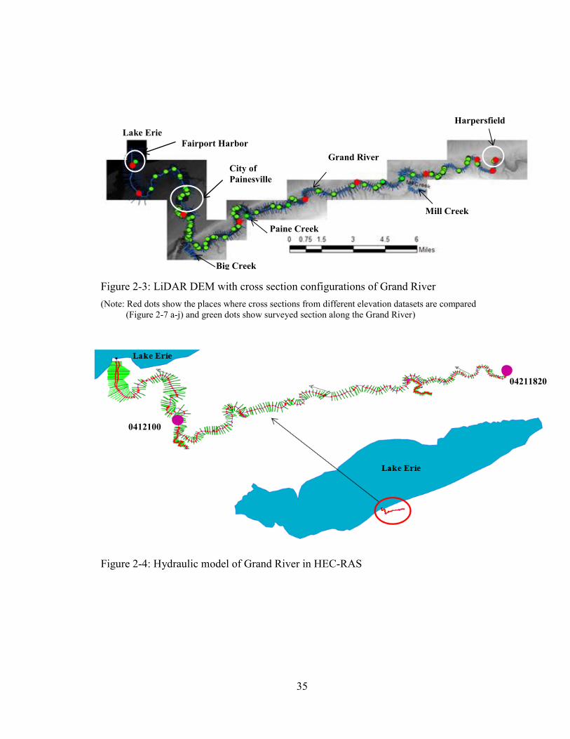
Figure 2-3: LiDAR DEM with cross section configurations of Grand River (Note: Red dots show the places where cross sections from different elevation datasets are compared
(Figure 2-7 a-j) and green dots show surveyed section along the Grand River)
Figure 2-4: Hydraulic model of Grand River in HEC-RAS
Harpersfield
Mill Creek
Grand River
Paine Creek
Big Creek
Lake Erie
City of Painesville
Fairport Harbor
04211820
0412100
36
a) Calibration of stage from 3/1/1996 to 03/31/1996
b) Calibration of stage from 4/15/1996 to 5/14/1996
c) Validation of stage from 3/5/1997 to 3/19/1997
Figure 2-5: Calibration of stage from 3/1/1996 to 3/31/1996 (a), 4/15/1996 to 5/14/1996 (b), and validation from 3/5/1997 to 3/19/1997 (c) at upstream gage station 04211820
734
736
738
740
742
Stag
e (f
t)
Date
Observed stageSimulated stage
732735738741744747
Stag
e (f
t)
Date
Observed stageSimulated stage
736
738
740
742
Stag
e (f
t)
Date
Observed stageSimulated stage
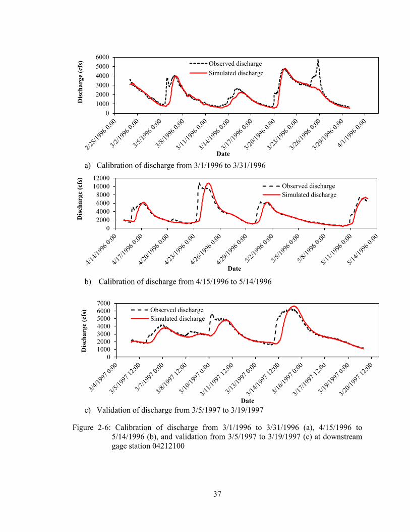
37
a) Calibration of discharge from 3/1/1996 to 3/31/1996
b) Calibration of discharge from 4/15/1996 to 5/14/1996
c) Validation of discharge from 3/5/1997 to 3/19/1997
Figure 2-6: Calibration of discharge from 3/1/1996 to 3/31/1996 (a), 4/15/1996 to 5/14/1996 (b), and validation from 3/5/1997 to 3/19/1997 (c) at downstream gage station 04212100
0100020003000400050006000
Disc
harg
e (c
fs)
Date
Observed dischargeSimulated discharge
02000400060008000
1000012000
Disc
harg
e (c
fs)
Date
Observed dischargeSimulated discharge
01000200030004000500060007000
Dis
char
ge (c
fs)
Date
Observed dischargeSimulated discharge
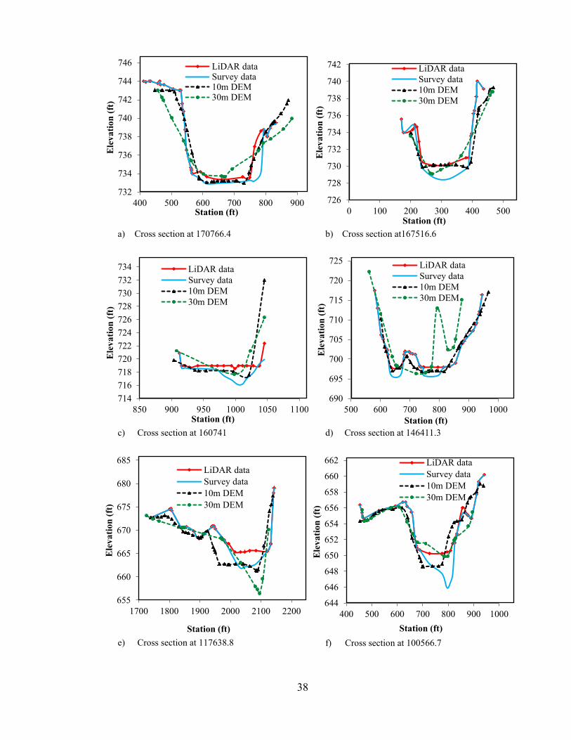
38
a) Cross section at 170766.4
b) Cross section at167516.6
c) Cross section at 160741
d) Cross section at 146411.3
e) Cross section at 117638.8
f) Cross section at 100566.7
732
734
736
738
740
742
744
746
400 500 600 700 800 900
Ele
vatio
n (f
t)
Station (ft)
LiDAR dataSurvey data10m DEM30m DEM
726
728
730
732
734
736
738
740
742
0 100 200 300 400 500
Ele
vatio
n (f
t)
Station (ft)
LiDAR dataSurvey data10m DEM30m DEM
714716718720722724726728730732734
850 900 950 1000 1050 1100
Ele
vatio
n (f
t)
Station (ft)
LiDAR dataSurvey data10m DEM30m DEM
690
695
700
705
710
715
720
725
500 600 700 800 900 1000
Ele
vatio
n (f
t)
Station (ft)
LiDAR dataSurvey data10m DEM30m DEM
655
660
665
670
675
680
685
1700 1800 1900 2000 2100 2200
Ele
vatio
n (f
t)
Station (ft)
LiDAR dataSurvey data10m DEM30m DEM
644
646
648
650
652
654
656
658
660
662
400 500 600 700 800 900 1000
Ele
vatio
n (f
t)
Station (ft)
LiDAR dataSurvey data10m DEM30m DEM
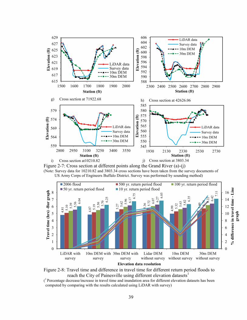
39
Figure 2-7: Cross section at different points along the Grand River (a)-(j) (Note: Survey data for 10210.82 and 3803.34 cross sections have been taken from the survey documents of
US Army Corps of Engineers Buffalo District. Survey was performed by sounding method)
Figure 2-8: Travel time and difference in travel time for different return period floods to
reach the City of Painesville using different elevation datasets1 (1 Percentage decrease/increase in travel time and inundation area for different elevation datasets has been computed by comparing with the results calculated using LiDAR with survey)
4.81
4.87
5.27
5.36
4.99
5.40
5.10
5.19
5.62
5.72
5.32
5.74
5.39
5.50
5.96
6.07
5.63
6.22
5.56
5.70
6.17
6.27
5.82
6.42
6.04
6.25
6.75
6.85
6.35
7.11
0
2
4
6
8
10
12
14
16
0
1
2
3
4
5
6
7
8
LiDAR withsurvey
10m DEM withsurvey
30m DEM withsurvey
Lidar DEMwithout survey
10m DEMwithout survey
30m DEMwithout survey
% d
iffer
ence
in tr
avel
tim
e - L
ine
grap
h
Tra
vel t
ime
(hrs
) -B
ar g
raph
Elevation data resolution
2006 flood 500 yr. return period flood 100 yr. return period flood50 yr. return period flood 10 yr. return period flood
g) Cross section at 71922.68
h) Cross section at 42626.06
i) Cross section at10210.82 j) Cross section at 3803.34
615617619621623625627629
1500 1600 1700 1800 1900 2000
Ele
vatio
n (f
t)
Station (ft)
LiDAR dataSurvey data10m DEM30m DEM
588590592594596598600602604606
2300 2400 2500 2600 2700 2800 2900
Ele
vatio
n (f
t)
Station (ft)
LiDAR dataSurvey data10m DEM30m DEM
559
564
569
574
579
2800 2950 3100 3250 3400 3550
Elev
atio
n (f
t)
Station (ft)
LiDAR dataSurvey data10m DEM30m DEM
545550555560565570575580585
1930 2130 2330 2530 2730
Ele
vatio
n (f
t)
Station (ft)
LiDAR dataSurvey data10m DEM30m DEM
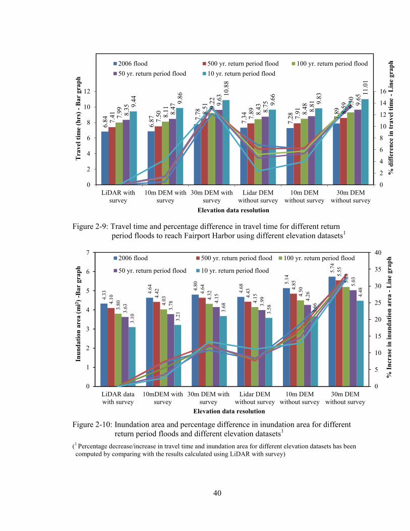
40
Figure 2-9: Travel time and percentage difference in travel time for different return
period floods to reach Fairport Harbor using different elevation datasets1
Figure 2-10: Inundation area and percentage difference in inundation area for different return period floods and different elevation datasets1
(1 Percentage decrease/increase in travel time and inundation area for different elevation datasets has been computed by comparing with the results calculated using LiDAR with survey)
6.84
6.87
7.78
7.34
7.28
7.89
7.41
7.50
8.51
7.89
7.91
8.59
7.99
8.11
9.22
8.43
8.48
9.30
8.35
8.47
9.63
8.75
8.81
9.65
9.44
9.86
10.8
8
9.66
9.83
11.0
1
0
2
4
6
8
10
12
14
16
0
2
4
6
8
10
12
LiDAR withsurvey
10m DEM withsurvey
30m DEM withsurvey
Lidar DEMwithout survey
10m DEMwithout survey
30m DEMwithout survey
% d
iffer
ence
in tr
avel
tim
e - L
ine
grap
h
Tra
vel t
ime
(hrs
) - B
ar g
raph
Elevation data resolution
2006 flood 500 yr. return period flood 100 yr. return period flood50 yr. return period flood 10 yr. return period flood
4.33
4.64
4.80
4.68
5.14
5.74
4.10
4.42
4.64
4.43
4.85
5.55
3.80
4.03
4.32
4.15
4.50
5.20
3.63
3.78
4.15
3.99
4.26
5.03
3.10
3.21
3.68
3.58
3.66
4.48
0
5
10
15
20
25
30
35
40
0
1
2
3
4
5
6
7
LiDAR datawith survey
10mDEM withsurvey
30m DEM withsurvey
Lidar DEMwithout survey
10m DEMwithout survey
30m DEMwithout survey
% In
cras
e in
inun
datio
n ar
ea -
Line
gra
ph
Inun
datio
n ar
ea (m
i2 ) -B
ar g
raph
Elevation data resolution
2006 flood 500 yr. return period flood 100 yr. return period flood
50 yr. return period flood 10 yr. return period flood
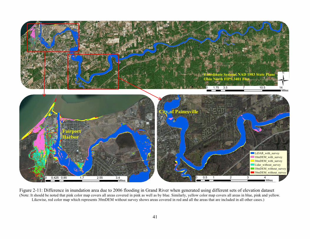
Ü
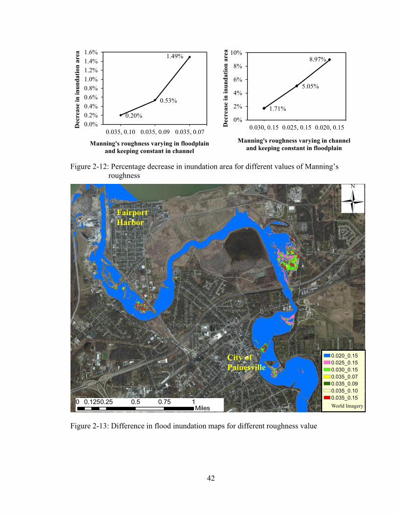
42
Figure 2-12: Percentage decrease in inundation area for different values of Manning’s roughness
Figure 2-13: Difference in flood inundation maps for different roughness value
0.20%
0.53%
1.49%
0.0%0.2%0.4%0.6%0.8%1.0%1.2%1.4%1.6%
0.035, 0.10 0.035, 0.09 0.035, 0.07
Dec
reas
e in
inun
datio
n ar
ea
Manning's roughness varying in floodplain and keeping constant in channel
1.71%
5.05%
8.97%
0%
2%
4%
6%
8%
10%
0.030, 0.15 0.025, 0.15 0.020, 0.15Dec
reas
e in
inun
datio
n ar
ea
Manning's roughness varying in channel and keeping constant in floodplain
Fairport Harbor
City of Painesville
0 0.25 0.5 0.75 10.125Miles
Ü
0.020_0.150.025_0.150.030_0.150.035_0.070.035_0.090.035_0.100.035_0.15World Imagery
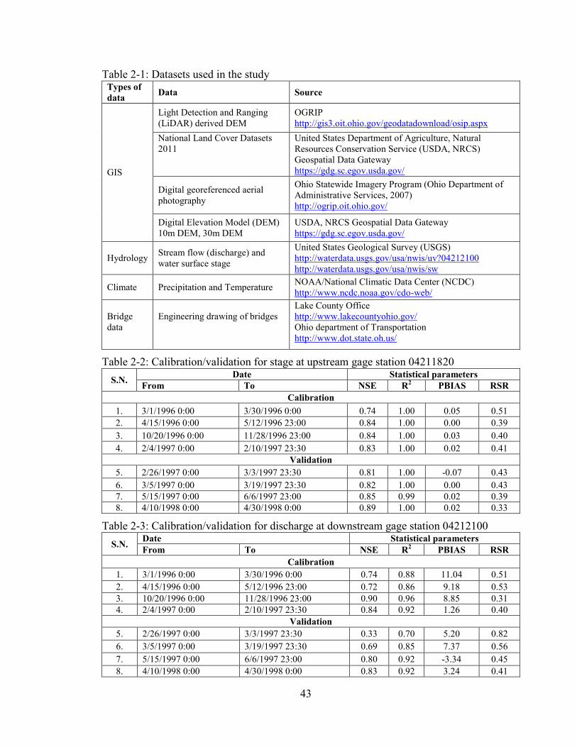
43
Table 2-1: Datasets used in the study Types of data Data Source
GIS
Light Detection and Ranging (LiDAR) derived DEM
OGRIP http://gis3.oit.ohio.gov/geodatadownload/osip.aspx
National Land Cover Datasets 2011
United States Department of Agriculture, Natural Resources Conservation Service (USDA, NRCS) Geospatial Data Gateway https://gdg.sc.egov.usda.gov/
Digital georeferenced aerial photography
Ohio Statewide Imagery Program (Ohio Department of Administrative Services, 2007) http://ogrip.oit.ohio.gov/
Digital Elevation Model (DEM) 10m DEM, 30m DEM
USDA, NRCS Geospatial Data Gateway https://gdg.sc.egov.usda.gov/
Hydrology Stream flow (discharge) and water surface stage
United States Geological Survey (USGS) http://waterdata.usgs.gov/usa/nwis/uv?04212100 http://waterdata.usgs.gov/usa/nwis/sw
Climate Precipitation and Temperature NOAA/National Climatic Data Center (NCDC) http://www.ncdc.noaa.gov/cdo-web/
Bridge data
Engineering drawing of bridges
Lake County Office http://www.lakecountyohio.gov/ Ohio department of Transportation http://www.dot.state.oh.us/
Table 2-2: Calibration/validation for stage at upstream gage station 04211820 S.N. Date Statistical parameters
From To NSE R2 PBIAS RSR Calibration
1. 3/1/1996 0:00 3/30/1996 0:00 0.74 1.00 0.05 0.51 2. 4/15/1996 0:00 5/12/1996 23:00 0.84 1.00 0.00 0.39 3. 10/20/1996 0:00 11/28/1996 23:00 0.84 1.00 0.03 0.40 4. 2/4/1997 0:00 2/10/1997 23:30 0.83 1.00 0.02 0.41
Validation 5. 2/26/1997 0:00 3/3/1997 23:30 0.81 1.00 -0.07 0.43 6. 3/5/1997 0:00 3/19/1997 23:30 0.82 1.00 0.00 0.43 7. 5/15/1997 0:00 6/6/1997 23:00 0.85 0.99 0.02 0.39 8. 4/10/1998 0:00 4/30/1998 0:00 0.89 1.00 0.02 0.33
Table 2-3: Calibration/validation for discharge at downstream gage station 04212100 S.N. Date Statistical parameters
From To NSE R2 PBIAS RSR Calibration
1. 3/1/1996 0:00 3/30/1996 0:00 0.74 0.88 11.04 0.51 2. 4/15/1996 0:00 5/12/1996 23:00 0.72 0.86 9.18 0.53 3. 10/20/1996 0:00 11/28/1996 23:00 0.90 0.96 8.85 0.31 4. 2/4/1997 0:00 2/10/1997 23:30 0.84 0.92 1.26 0.40
Validation 5. 2/26/1997 0:00 3/3/1997 23:30 0.33 0.70 5.20 0.82 6. 3/5/1997 0:00 3/19/1997 23:30 0.69 0.85 7.37 0.56 7. 5/15/1997 0:00 6/6/1997 23:00 0.80 0.92 -3.34 0.45 8. 4/10/1998 0:00 4/30/1998 0:00 0.83 0.92 3.24 0.41
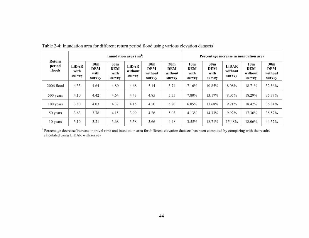
44
Table 2-4: Inundation area for different return period flood using various elevation datasets1
Return period floods
Inundation area (mi2) Percentage increase in inundation area
LiDAR with
survey
10m DEM with
survey
30m DEM with
survey
LiDAR without survey
10m DEM
without survey
30m DEM
without survey
10m DEM with
survey
30m DEM with
survey
LiDAR without survey
10m DEM
without survey
30m DEM
without survey
2006 flood 4.33 4.64 4.80 4.68 5.14 5.74 7.16% 10.85% 8.08% 18.71% 32.56%
500 years 4.10 4.42 4.64 4.43 4.85 5.55 7.80% 13.17% 8.05% 18.29% 35.37%
100 years 3.80 4.03 4.32 4.15 4.50 5.20 6.05% 13.68% 9.21% 18.42% 36.84%
50 years 3.63 3.78 4.15 3.99 4.26 5.03 4.13% 14.33% 9.92% 17.36% 38.57%
10 years 3.10 3.21 3.68 3.58 3.66 4.48 3.55% 18.71% 15.48% 18.06% 44.52%
1 Percentage decrease/increase in travel time and inundation area for different elevation datasets has been computed by comparing with the results calculated using LiDAR with survey
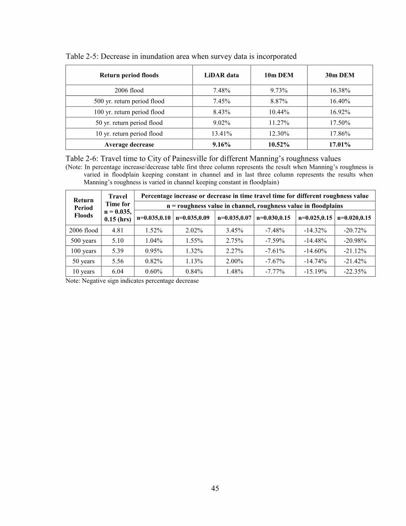
45
Table 2-5: Decrease in inundation area when survey data is incorporated
Return period floods LiDAR data 10m DEM 30m DEM
2006 flood 7.48% 9.73% 16.38% 500 yr. return period flood 7.45% 8.87% 16.40% 100 yr. return period flood 8.43% 10.44% 16.92% 50 yr. return period flood 9.02% 11.27% 17.50% 10 yr. return period flood 13.41% 12.30% 17.86%
Average decrease 9.16% 10.52% 17.01%
Table 2-6: Travel time to City of Painesville for different Manning’s roughness values (Note: In percentage increase/decrease table first three column represents the result when Manning’s roughness is
varied in floodplain keeping constant in channel and in last three column represents the results when Manning’s roughness is varied in channel keeping constant in floodplain)
Return Period Floods
Travel Time for n = 0.035, 0.15 (hrs)
Percentage increase or decrease in time travel time for different roughness value n = roughness value in channel, roughness value in floodplains
n=0.035,0.10 n=0.035,0.09 n=0.035,0.07 n=0.030,0.15 n=0.025,0.15 n=0.020,0.15
2006 flood 4.81 1.52% 2.02% 3.45% -7.48% -14.32% -20.72% 500 years 5.10 1.04% 1.55% 2.75% -7.59% -14.48% -20.98% 100 years 5.39 0.95% 1.32% 2.27% -7.61% -14.60% -21.12% 50 years 5.56 0.82% 1.13% 2.00% -7.67% -14.74% -21.42% 10 years 6.04 0.60% 0.84% 1.48% -7.77% -15.19% -22.35%
Note: Negative sign indicates percentage decrease
46
Chapter 3. Development of a Flood Warning System and Flood Inundation Mapping for the Grand River near the City of Painesville, Ohio
Abstract Flooding is one of the most frequent natural disasters across the world, which
damages properties and may take the lives of people. Flood warning system can play
significant roles to minimize those effects by evacuating the people from the probable
affected areas during the peak flood time. Therefore, the major objective of this research
is to prepare flood warning system for the Grand River, Ohio to provide evacuation
period for the people of probable affected areas with sufficient lead time. Flood warning
system was developed by calculating flood travel time and generating the inundation
mapping for 12 different selected flood stages, which were approximately 2 to 500 years
in recurrence interval, ranging from 10.00 ft to 21.00 ft at gage station 04212100, near
the City of Painesville. A one-dimensional model, Hydraulic Engineering Center-River
Analysis System (HEC-RAS) was utilized for hydraulic modeling. Geospatial data
required for HEC-RAS were obtained using Digital Elevation Model (DEM) derived
from Light Detection and Ranging (LiDAR) datasets, which was pre-processed and post
processed in HEC-GeoRAS to produce flood inundation maps. The flood travel time and
flood inundation maps have been generated integrating LiDAR data with field verified
survey and calibrated Manning’s roughness value. The generated inundation maps
estimate the aerial extent of flooding along the Grand River corresponding to the various
flood stages at gage station 04212100 near the City of Painesville and 04211820 in
Harpersfield. The inundation maps were overlaid on digital orthographic maps to
visualize its aerial extents. The steady state hydraulic model was calibrated using
available datasets. There are more than 100 houses, many roads, bridges and parks along
47
the Grand River are vulnerable to flooding during 500 year return period flood leading to
the requirement of a flood warning system to be installed near the City of Painesville,
Ohio.
Keywords: Flood Warning System, Inundation Mapping, HEC-RAS, HEC-GeoRAS,
LiDAR datasets
Introduction
Flooding is a major natural hazard which greatly impacts different regions across
the world (Yuan et al., 2011; Alfaro et al., 2013). Ludlum (1991) defines a flood as the
presence of “too much water in areas that are not normally under water”. Similarly,
Standard Flood Insurance Policy (SFIP) defines flood as “A general and temporary
condition of partial or complete inundation of two or more acres of normally dry land
area of two or more properties (at least one of which is your property) from overflow of
inland or tidal waters from any source, or from mudflow” (FEMA, 2001a). In the United
States, flood takes the lives of more people than any form of other natural disaster
(Krimm, 1996; Perry 2000). Among the various types of flood, flash floods are the most
dangerous as these are the primary cause of deaths in the United States which kill more
than 140 people each year (NWS, 2016). Flash flood is an abrupt flow of a large amount
of water in a river within a few minutes or hours due to extreme rainfall, failure of a
dam/levee or an abrupt release of water due to ice jam (NWS, 2016; Mwape, 2009).
The City of Painesville has been frequently threatened by flooding over different
years such as in 1986, 1989, 2006, 2008, and 2011. The historical annual peak flow/stage
and various flood stage level as per National Weather Service (NWS, 2016a) in the
Grand River, Ohio is shown in Figure 3-1. The extensive flooding in Grand River, Ohio
48
was experienced on July 27-28, 2006 due to the intense rainfall of more than 11 inches
depth that occurred within a short period of time. This was one of the highest historical
flood occurred in the Grand River, near the City of Painesville. This flood led to the
property damages estimated of 30 million USD and one fatality in Lake County. Several
people (600) had to be evacuated due to which three counties (Lake, Geauga and
Ashtabula) were declared as Federal and State disaster areas (Ebner et al. 2007). The
flood destroyed more than 800 homes and 5 bridges in Lake County. Additionally, it
disrupted traffic by closing 13 roads near the City of Painesville. The peak discharge and
stage for that event was estimated to be 35,000 cfs and 19.35 ft. respectively (Figure 3-2)
as recorded by USGS gauge station (04212100) near the City of Painesville. Therefore,
the development of flood warning system in the Grand River is absolutely essential to
protect the lives of people and reduce the property losses.
Flood warning system protects people’s lives and prevents property damages from
such disaster by providing the sufficient lead time for the evacuation (Krzysztofowicz et
al., 1994). The formal UN report (ISDR, 2003) defines early warning system as “The
provision of timely and effective information, through identifying institutions that allow
individuals exposed to a hazard to take action to avoid or reduce their risk and prepare for
effective response”. Flood risk management should contain efficient actions of
preparedness, response and recovery, which is essential for rescue operation during flood
time (Borga et al., 2011). For the efficient management of flood risks, two important
factors that should be taken into well are flood travel time and possible area of
inundation. Flood travel time is the key element needed for the timely evacuation of
people from probable flood prone areas. Likewise, flood inundation maps are also
49
important tools that represent spatial variability of flood hazard and provide the clear
picture and robust understanding of floods than any other forms (Merz et al., 2007;
Leedal et al., 2010). Therefore, these maps should be carefully prepared and made easily
accessible to the public without any difficulties (Holtzclaw et al., 2005). Moreover, it is
essential to have a proper communication and coordination among federal, regional, state
and local bodies and the private sectors to establish effective flood warning system
(Fukuoka, 1998).
There are some basic processes before and after the flood occurrence, which
should be followed while developing the efficient flood warning system (Aliasgar, 2012;
ISDR PPEW, 2006). The processes before the flood occurrence are: generation of flood
inundation maps for various flood stages, quantification of thresholds in maps and
identification of flood hazard areas for different flood scenarios. Similarly, the processes
after the flood occurrence are: to inform concerned officials/authorities, issue warning
system to the people of possible inundation areas, evacuate people from probable
inundation areas, and rescue operation. However, both the citizens and concerned
authorities should be able to understand the risks associated with the floods in order to
minimize the effects of flood hazards in any area (Holtzclaw, 2005). Also, the
communities should be involved in Federal Emergency Management Agency (FEMA)
Map Modernization program (Holtzclaw, 2005) to understand the flood maps and
warning system developed by FEMA.
The primary objective of this research was to develop a hydraulic model using
HEC-RAS for the use by the National Weather Service and prepare all necessary digital
files including rating curve to provide the evacuation time for flood warning system in
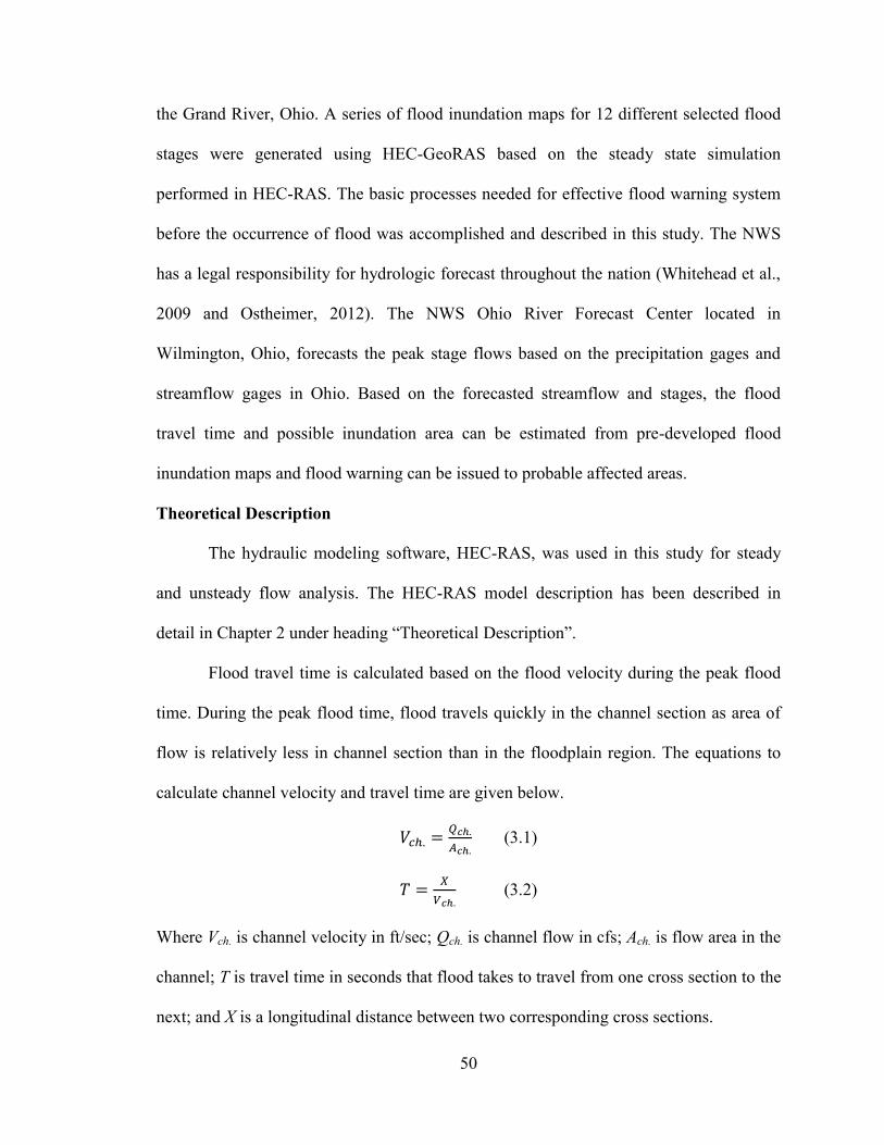
50
the Grand River, Ohio. A series of flood inundation maps for 12 different selected flood
stages were generated using HEC-GeoRAS based on the steady state simulation
performed in HEC-RAS. The basic processes needed for effective flood warning system
before the occurrence of flood was accomplished and described in this study. The NWS
has a legal responsibility for hydrologic forecast throughout the nation (Whitehead et al.,
2009 and Ostheimer, 2012). The NWS Ohio River Forecast Center located in
Wilmington, Ohio, forecasts the peak stage flows based on the precipitation gages and
streamflow gages in Ohio. Based on the forecasted streamflow and stages, the flood
travel time and possible inundation area can be estimated from pre-developed flood
inundation maps and flood warning can be issued to probable affected areas.
Theoretical Description
The hydraulic modeling software, HEC-RAS, was used in this study for steady
and unsteady flow analysis. The HEC-RAS model description has been described in
detail in Chapter 2 under heading “Theoretical Description”.
Flood travel time is calculated based on the flood velocity during the peak flood
time. During the peak flood time, flood travels quickly in the channel section as area of
flow is relatively less in channel section than in the floodplain region. The equations to
calculate channel velocity and travel time are given below.
𝑉𝑐ℎ. =𝑄𝑐ℎ.
𝐴𝑐ℎ. (3.1)
𝑇 =𝑋
𝑉𝑐ℎ. (3.2)
Where Vch. is channel velocity in ft/sec; Qch. is channel flow in cfs; Ach. is flow area in the
channel; T is travel time in seconds that flood takes to travel from one cross section to the
next; and X is a longitudinal distance between two corresponding cross sections.
51
Rating curve was used to calculate the streamflow for various stages. Rating
curve equation was developed using the daily discharge data greater than 75 percentile
for the period of 1988-2005. Since all the practical purposes of developing rating curve in
this study was to estimate the streamflow during high flood time, rating curve was
developed using 75 percentile flow in order to capture all high flood discharge values. It
is noteworthy to mention that the rating curve developed for higher flow may not be
applicable during low flow condition and vice versa.
Materials and Methodology
Study Area
This study was conducted in the Grand River watershed, which is located in the
Northeastern region of Ohio. The City of Painesville along the Grand River is one of the
most affected regions due to frequent flooding that occurred from time to time (2006,
2008, and 2011). The detail description of the Grand River watershed is already
described in Chapter 2.
Overall Flood Warning Approach
Basically, an approach towards a better flood warning system was developed in
this study. The following steps will be accomplished to develop fully functional flood
warning system. This approach is the similar to the approach adopted in Findlay County
(Whitehead, 2009) and Licking County (Ostheimer, 2012) of Ohio warning system has
been developed.
Development of a Hydraulic Model
Fully functional HEC-RAS model was developed in this study. The
calibrated/validated unsteady HEC-RAS model developed in Chapter 2 was used to run
52
the hydraulic simulation. The overall modeling approach for calibration and validation of
Manning’s roughness has been already described in Chapter 2 under heading “Overall
Modeling Approach”. The model was further calibrated for steady flow scenario using
high-water mark profiles of 2006 flood. This hydraulic model will be shared with NWS
so that they can utilize to simulate and generate inundation maps for other various flow
scenarios.
Development of Rating Curve
Rating curve was developed for high flow periods for the streamgage 04212100
near the City of Painesville. The developed rating curve was utilized to predict the flood
discharge for 12 different selected floods in the Grand River to be used in hydraulic
model.
Preparation of Digital Flood Inundation Maps
The digital flood inundation maps for 12 different selected flood stages were
generated using HEC-GeoRAS software based on the steady flow simulation performed
in HEC-RAS. The digital flood inundation maps were generated based on the upstream
and downstream gage height. These digital maps could be uploaded online in National
Portal System or Regional Portal System after further refinement to provide the real time
flood inundation to the people.
Installation of Siren System
For the effective flood warning approach, the siren system could be installed at
various suitable locations near the City of Painesville to warn the people before the flood
affects the probable areas along the Grand River.
53
Evacuation Time
The flood travel time for 12 different flood scenarios were calculated based on the
hydraulic simulation in HEC-RAS. These flood travel time can be used for evacuation of
people from probable inundation areas.
This approach provides the valuable information to the public regarding
evacuation time and probable inundation areas for several flood stages. Hence, this
information can be used to relocate people in safer places with sufficient lead time.
However, in order to develop a fully automated flood warning system, streamgages in
various required places with automated equipment are necessary to be installed, which
will be discussed later in the recommendation section.
HEC-GeoRAS/HEC-RAS Model Input
The HEC-RAS model was developed using LiDAR with field survey data. The
summary of input data and detail description of HEC-GeoRAS/HEC-RAS model inputs
are discussed in Chapter 2.
Model Calibration and Validation
The unsteady HEC-RAS model was calibrated through the iterative process to
obtain the realistic value of Manning’s roughness, which was accomplished by
comparing observed stage/discharge with the simulated stage/discharge. The model
calibration and validation has been described in Chapter 2 under heading “Model
Calibration and Validation”.
Typically, steady HEC-RAS model is calibrated using high-water mark profiles
obtained from the survey during the flood time (Dewberry & Davis, 2002). In this study,
the high-water mark elevation points were compared with the modeled water surface
54
elevation points to evaluate the model efficiency. USGS conducted a survey to obtain
high-water mark profiles along the Grand River using standard surveying technique
during 2006 flood, and those high-water mark elevation points for this study were
collected from Ebner et al. (2007). However, the surveyed data of high-water marks may
not always be accurate especially debris and sediments may not be available during the
time of the high flood (Ebner et al., 2007).
Model Evaluation Criteria
Various statistical parameters such as NSE, R2, PBIAS, and RMSE were used to
check the accuracy and predictive power of the model, which have been described in
detail in Chapter 2 under heading “Model Evaluation Criteria”.
Results and Discussions
Unsteady Flow Scenario
The unsteady model was calibrated and validated for both stage and discharge.
The performance of the model was good in calibration and validation for different time
periods of 1996-1998, which was evaluated using statistical parameter and visual
inspection method. The detail calibration and validation of unsteady hydraulic model
have been described in Chapter 2 under heading “Results and Discussion”.
Steady Flow Scenario
The steady flow model was calibrated to match the high-water mark profiles of
2006 flood. The drainage area ratio method was used to estimate the discharge of all three
creeks because of unavailability of gage readings. The streamflow data for all rivers that
were taken in consideration are shown in Table 3-1. The high-water mark profiles were
compared with simulated water surface elevation for 2006 flood in the Grand River in 19
55
locations, which are presented in Table 3-2. The errors associated with water surface
elevation ranged from 0.02 ft to 1.75 ft. The errors were less than 1 ft in 12 different
locations and within 1.36 ft for most of the locations.
Rating Curve
Rating curve for streamgage near the City of Painesville was developed using 75
percentile exceedance discharge values for the period of 1988-2005 in order to capture all
the high flood discharge values (Figure 3-3). The equation of developed rating curve is
given below.
𝑄 = 166.67 𝐻1.7971 (3.6)
Where Q is flow discharge (cfs) and H is the stage (ft) of water in the river.
The developed rating curve was validated from the period of January 2006 to
January 2015 with NSE of 0.91 (Figure 3-4). However, the rating curve developed using
entire datasets under-predicted the high flow, especially during flood period. This is not
surprising as the channel section representing the stage discharge relationship varies
depending upon the flood stage; therefore, the rating curve developed for low flood stage
may not necessarily true for the higher flood stage.
Calculation of Travel Time and Development of Profiles/Flood-inundation maps
The simulation was performed in steady state condition to generate the profile for
12 stages from 10 ft to 21 ft with 1 ft increment at the Grand River near the City of
Painesville. However, 19.35 ft was selected instead of 19.00 ft. in order to represent the
flood of July 2006, which approximately corresponds to the flood of 500 years return
period. Discharge values corresponding to the selected stages were calculated using the
rating curve developed at station 04212100. As there were no any recorded flows in
56
tributaries of the Grand River including Mill, Paine and Big Creek, discharges for various
selected stages for those tributaries were estimated using simple drainage area ratio. The
estimated streamflow data for selected stages are presented in Table 3-1. The water
surface extents modeled in HEC-RAS were then transferred to HEC-GeoRAS for the
development of flood inundation maps for those selected stages. The flood inundation
maps were then superimposed onto digital imagery maps produced by Ohio
Geographically Referenced Information Program (OGRIP) to see the aerial extents of
flooding. The generated inundation maps for 12 different selected stages are presented in
appendices section of this chapter.
Flood travel time to reach the City of Painesville and Fairport Harbor including
the flood inundation areas were calculated for various flood stages at gage station
04212100, near the City of Painesville (Figure 3-5). The equations for calculated travel
time and predicted inundation area were also developed so that they could be used to
estimate travel time and inundation area for other flood stages (Figure 3-5).
Flood Damages along the Grand River
Many houses, apartments, roads, bridges and parks along the Grand River are
more susceptible to flooding due to 500 years return period flood as shown in the study
area. The flood inundation map corresponding to 500 year return period flood is shown in
Figure 3-X in appendices section. Since this study was particularly focused in the City of
Painesville, several houses, bridges and parks along the Grand River, beyond the study
area, which are susceptible to flooding might have been excluded here. The detail
information can be obtained from the flood map attached in appendices section for 19.35
ft stage at gage station 04212100. The major affected areas according to hydraulic
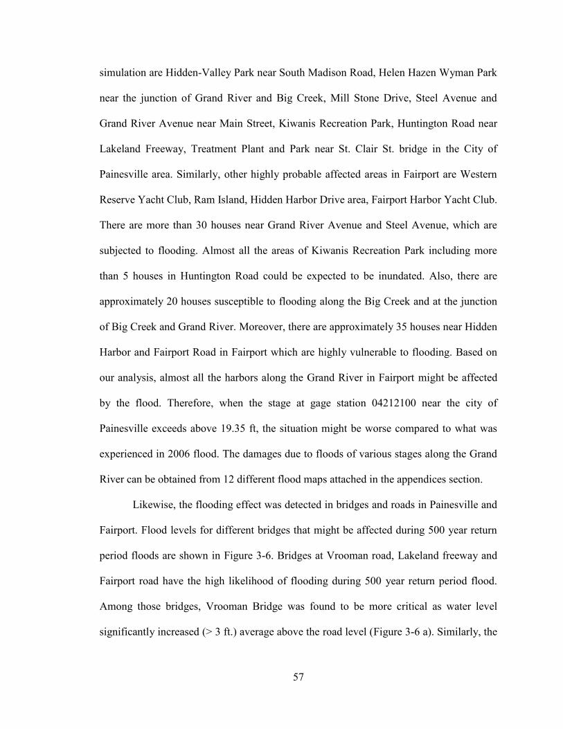
57
simulation are Hidden-Valley Park near South Madison Road, Helen Hazen Wyman Park
near the junction of Grand River and Big Creek, Mill Stone Drive, Steel Avenue and
Grand River Avenue near Main Street, Kiwanis Recreation Park, Huntington Road near
Lakeland Freeway, Treatment Plant and Park near St. Clair St. bridge in the City of
Painesville area. Similarly, other highly probable affected areas in Fairport are Western
Reserve Yacht Club, Ram Island, Hidden Harbor Drive area, Fairport Harbor Yacht Club.
There are more than 30 houses near Grand River Avenue and Steel Avenue, which are
subjected to flooding. Almost all the areas of Kiwanis Recreation Park including more
than 5 houses in Huntington Road could be expected to be inundated. Also, there are
approximately 20 houses susceptible to flooding along the Big Creek and at the junction
of Big Creek and Grand River. Moreover, there are approximately 35 houses near Hidden
Harbor and Fairport Road in Fairport which are highly vulnerable to flooding. Based on
our analysis, almost all the harbors along the Grand River in Fairport might be affected
by the flood. Therefore, when the stage at gage station 04212100 near the city of
Painesville exceeds above 19.35 ft, the situation might be worse compared to what was
experienced in 2006 flood. The damages due to floods of various stages along the Grand
River can be obtained from 12 different flood maps attached in the appendices section.
Likewise, the flooding effect was detected in bridges and roads in Painesville and
Fairport. Flood levels for different bridges that might be affected during 500 year return
period floods are shown in Figure 3-6. Bridges at Vrooman road, Lakeland freeway and
Fairport road have the high likelihood of flooding during 500 year return period flood.
Among those bridges, Vrooman Bridge was found to be more critical as water level
significantly increased (> 3 ft.) average above the road level (Figure 3-6 a). Similarly, the
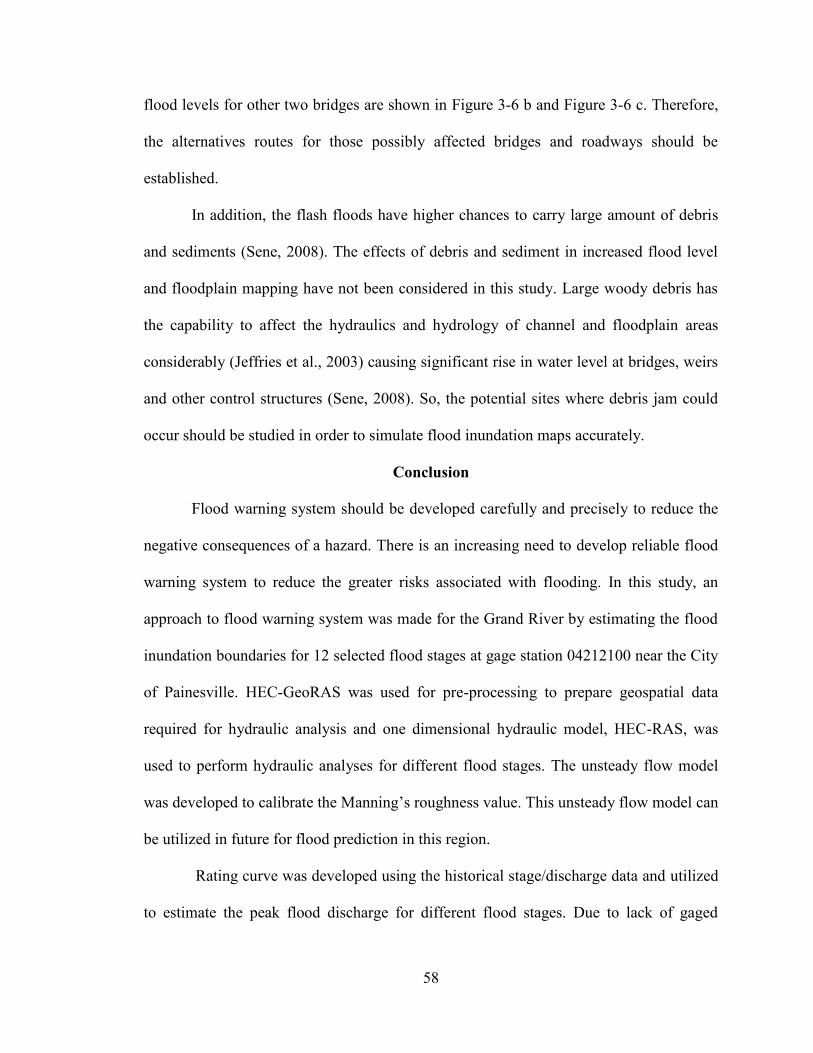
58
flood levels for other two bridges are shown in Figure 3-6 b and Figure 3-6 c. Therefore,
the alternatives routes for those possibly affected bridges and roadways should be
established.
In addition, the flash floods have higher chances to carry large amount of debris
and sediments (Sene, 2008). The effects of debris and sediment in increased flood level
and floodplain mapping have not been considered in this study. Large woody debris has
the capability to affect the hydraulics and hydrology of channel and floodplain areas
considerably (Jeffries et al., 2003) causing significant rise in water level at bridges, weirs
and other control structures (Sene, 2008). So, the potential sites where debris jam could
occur should be studied in order to simulate flood inundation maps accurately.
Conclusion
Flood warning system should be developed carefully and precisely to reduce the
negative consequences of a hazard. There is an increasing need to develop reliable flood
warning system to reduce the greater risks associated with flooding. In this study, an
approach to flood warning system was made for the Grand River by estimating the flood
inundation boundaries for 12 selected flood stages at gage station 04212100 near the City
of Painesville. HEC-GeoRAS was used for pre-processing to prepare geospatial data
required for hydraulic analysis and one dimensional hydraulic model, HEC-RAS, was
used to perform hydraulic analyses for different flood stages. The unsteady flow model
was developed to calibrate the Manning’s roughness value. This unsteady flow model can
be utilized in future for flood prediction in this region.
Rating curve was developed using the historical stage/discharge data and utilized
to estimate the peak flood discharge for different flood stages. Due to lack of gaged
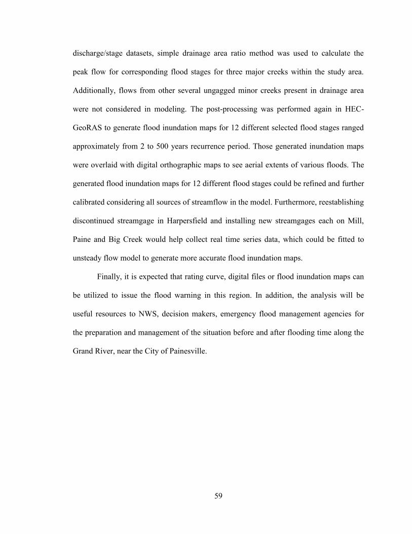
59
discharge/stage datasets, simple drainage area ratio method was used to calculate the
peak flow for corresponding flood stages for three major creeks within the study area.
Additionally, flows from other several ungagged minor creeks present in drainage area
were not considered in modeling. The post-processing was performed again in HEC-
GeoRAS to generate flood inundation maps for 12 different selected flood stages ranged
approximately from 2 to 500 years recurrence period. Those generated inundation maps
were overlaid with digital orthographic maps to see aerial extents of various floods. The
generated flood inundation maps for 12 different flood stages could be refined and further
calibrated considering all sources of streamflow in the model. Furthermore, reestablishing
discontinued streamgage in Harpersfield and installing new streamgages each on Mill,
Paine and Big Creek would help collect real time series data, which could be fitted to
unsteady flow model to generate more accurate flood inundation maps.
Finally, it is expected that rating curve, digital files or flood inundation maps can
be utilized to issue the flood warning in this region. In addition, the analysis will be
useful resources to NWS, decision makers, emergency flood management agencies for
the preparation and management of the situation before and after flooding time along the
Grand River, near the City of Painesville.
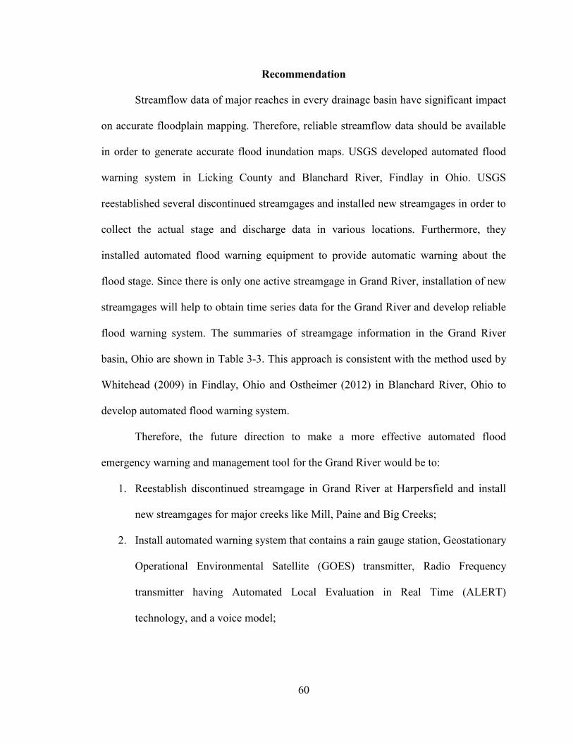
60
Recommendation
Streamflow data of major reaches in every drainage basin have significant impact
on accurate floodplain mapping. Therefore, reliable streamflow data should be available
in order to generate accurate flood inundation maps. USGS developed automated flood
warning system in Licking County and Blanchard River, Findlay in Ohio. USGS
reestablished several discontinued streamgages and installed new streamgages in order to
collect the actual stage and discharge data in various locations. Furthermore, they
installed automated flood warning equipment to provide automatic warning about the
flood stage. Since there is only one active streamgage in Grand River, installation of new
streamgages will help to obtain time series data for the Grand River and develop reliable
flood warning system. The summaries of streamgage information in the Grand River
basin, Ohio are shown in Table 3-3. This approach is consistent with the method used by
Whitehead (2009) in Findlay, Ohio and Ostheimer (2012) in Blanchard River, Ohio to
develop automated flood warning system.
Therefore, the future direction to make a more effective automated flood
emergency warning and management tool for the Grand River would be to:
1. Reestablish discontinued streamgage in Grand River at Harpersfield and install
new streamgages for major creeks like Mill, Paine and Big Creeks;
2. Install automated warning system that contains a rain gauge station, Geostationary
Operational Environmental Satellite (GOES) transmitter, Radio Frequency
transmitter having Automated Local Evaluation in Real Time (ALERT)
technology, and a voice model;

61
3. Collect high-water mark profiles during the peak flood time which could be used
for further calibration and validation of steady flow model for different floods;
4. Couple hydrological and hydraulic model that might lead to improved warning
system;
5. Develop two dimensional unsteady hydraulic models to understand the spatial
flooding pattern more effectively.
62
References:
Alfaro et al., “Design of an early warning flood level indicator” October 2013.
Aliasgar, Kelly. "Developing a geoinformatics based early warning system for floods in
the Caribbean, Trinidad and Tobago." (2012).
Borga, M., et al. "Flash flood forecasting, warning and risk management: the HYDRATE
project." Environmental Science & Policy 14.7 (2011): 834-844.
Dewberry & Davis, LLC. “Floodplain Modeling Manual; HEC-RAS Procedures for
HEC-2 Modelers” 2002; http://www.sciencedirect.com/science/article/pii/S01695
55X02003252
Ebner, Andrew D., et al. Flood of July 27-31, 2006, on the Grand River near Painesville,
Ohio. No. 2007-1164. Geological Survey (US), 2007.
FEMA. 2001a. Answers to Questions about the National Flood Insurance Program.
Federal Emergency Management Agency, Washington D.C.
FEMA, 2001a- National Weather Service’s FLDWAV Computer Program;
FEMA, 2001b Full Equations (FEQ) Model for the Solution of Full, Dynamic Equations
of Motion for One-Dimensional Unsteady Flow in Open Channels and Through
Control Structures.
Fukuoka, Shoji. "Floodplain risk management. Proceedings of an international workshop,
Hiroshima, Japan, 11-13 November 1996." Floodplain risk management.
Proceedings of an international workshop, Hiroshima, Japan, 11-13 November
1996.. AA Balkema, 1998.
Jeffries, Richard, Stephen E. Darby, and David A. Sear. "The influence of vegetation and
organic debris on flood-plain sediment dynamics: case study of a low-order
stream in the New Forest, England." Geomorphology51.1 (2003): 61-80.
Holtzclaw, Emily, Betty Leite, and Rick Myrick. "Floodplain modeling applications for
emergency management and stakeholder involvement a case study: New
Braunfels, Texas." (2005).

63
ISDR (UN International Strategy for Disaster Reduction), 2003: Terminology: Basic
terms of disaster risk reduction.
ISDR PPEW 2006, Basics of Early Warning, UNISDR, <
http://www.unisdr.org/ppew/whats-ew/basics-ew.htm.>.
Krimm, Richard W. "Reducing flood losses in the United States."Proceedings of
international workshop on floodplain risk management. < The> Committee of
International Workshop on Floodplain Risk Management, 1996.
Krzysztofowicz, Roman, Karen S. Kelly, and Dou Long. "Reliability of flood warning
systems." Journal of water resources planning and management120.6 (1994): 906-
926.
Leedal, David, et al., "Visualization approaches for communicating real-time flood
forecasting level and inundation information." Journal of Flood Risk
Management 3.2 (2010): 140-150.
Ludlum, David McWilliams. National Audubon Society Field Guide to North American
Weather. Vol. 18. Knopf, 1991.
Merz, Bruno, A. H. Thieken, and Martin Gocht. "Flood risk mapping at the local scale:
concepts and challenges." Flood risk management in Europe. Springer
Netherlands, 2007. 231-251.
Mwape YP (2009) An impact of floods on the socio-economic livelihoods of people: a
case study of Sikaunzwe Community in Kazungula District of Zambia. M.Sc.
Thesis, University of the Free State, South Africa
NWS, 2012; NOAA’s National Weather Service Flood Warning Systems Manual, U.S.
DEPARTMENT OF COMMERCE, NOAA-April, 2012
NWS, 2016. Flash Flooding-Flash Floods- The #1 Weather Related Killer in the United
States. (Accessed March 2016, at URL)
http://www.wrh.noaa.gov/psr/general/severe/ flashflood.php
NWS, 2016a. Advanced Hydrologic Prediction Service. (accessed March 2016)
http://water.weather.gov/ahps2/hydrograph.php?wfo=cle&gage=PNVO1

64
Ostheimer, Chad J. Development of a flood-warning system and flood-inundation
mapping in Licking County, Ohio. No. FHWA/OH-2012/4. US Department of the
Interior, US Geological Survey, 2012.
Perry, Charles A. Significant floods in the United States during the 20th century-USGS
measures a century of floods. No. 024-00. US Geological Survey,, 2000.Smemoe,
Chris, Jim Nelson, and Alan Zundel. "Developing a Probabilistic Flood Plain
Boundary Using HEC-1 and HEC-RAS." World Water & Environmental
Resources Congress 2003. ASCE, 2003.
Sene, Kevin. Flood warning, forecasting and emergency response. Springer Science &
Business Media, 2008.
United States Census Bureau, 2010 - http://quickfacts.census.gov/qfd/states/
39/3959416.html).
White, Gilbert F. Human adjustment to floods: a geographical approach to the flood
problem in the United States. No. 29. Chicago: University of Chicago, 1945.0
Whitehead, Matthew T., and Chad J. Ostheimer. Development of a Flood-Warning
System and Flood-Inundation Mapping for the Blanchard River in Findlay, Ohio.
2009.
Yuan et al., “Floodplain Modeling in the Kansas River Basin Using Hydrologic
Engineering Center (HEC) Models”. USEPA, NV, 2011
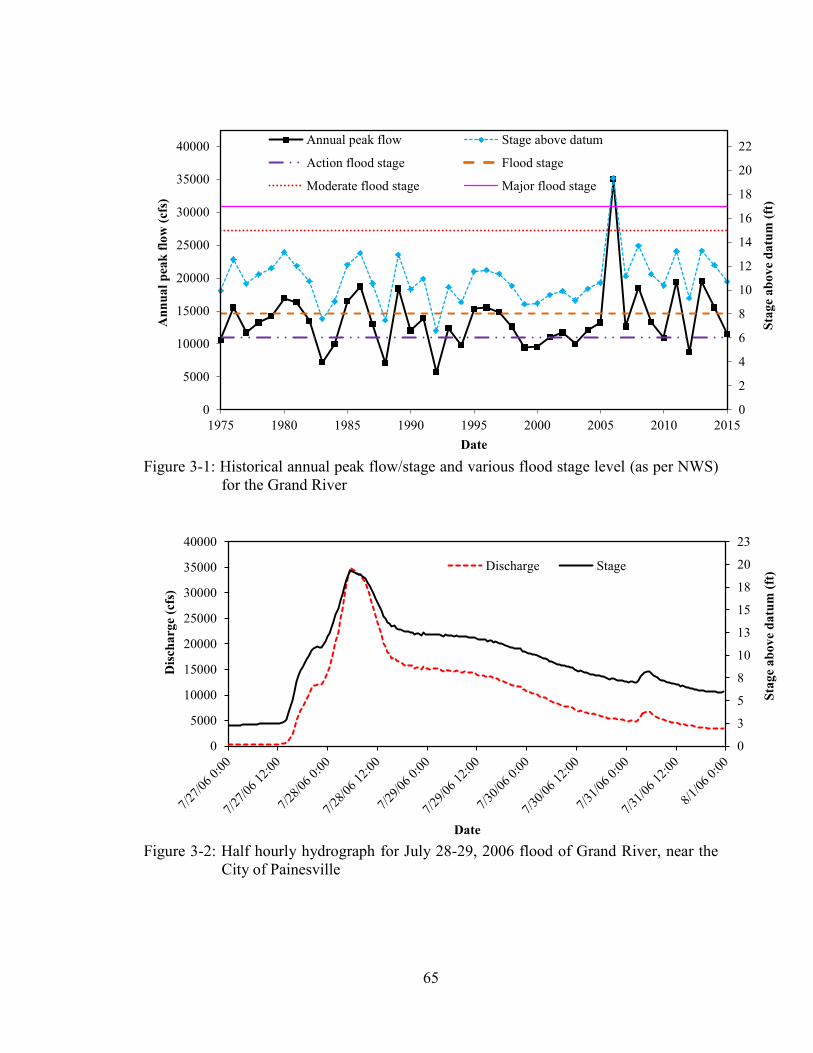
65
Figure 3-1: Historical annual peak flow/stage and various flood stage level (as per NWS)
for the Grand River
Figure 3-2: Half hourly hydrograph for July 28-29, 2006 flood of Grand River, near the City of Painesville
0
2
4
6
8
10
12
14
16
18
20
22
0
5000
10000
15000
20000
25000
30000
35000
40000
1975 1980 1985 1990 1995 2000 2005 2010 2015
Stag
e ab
ove
datu
m (f
t)
Ann
ual p
eak
flow
(cfs
)
Date
Annual peak flow Stage above datum
Action flood stage Flood stage
Moderate flood stage Major flood stage
0
3
5
8
10
13
15
18
20
23
0
5000
10000
15000
20000
25000
30000
35000
40000
Stag
e ab
ove
datu
m (f
t)
Dis
char
ge (c
fs)
Date
Discharge Stage
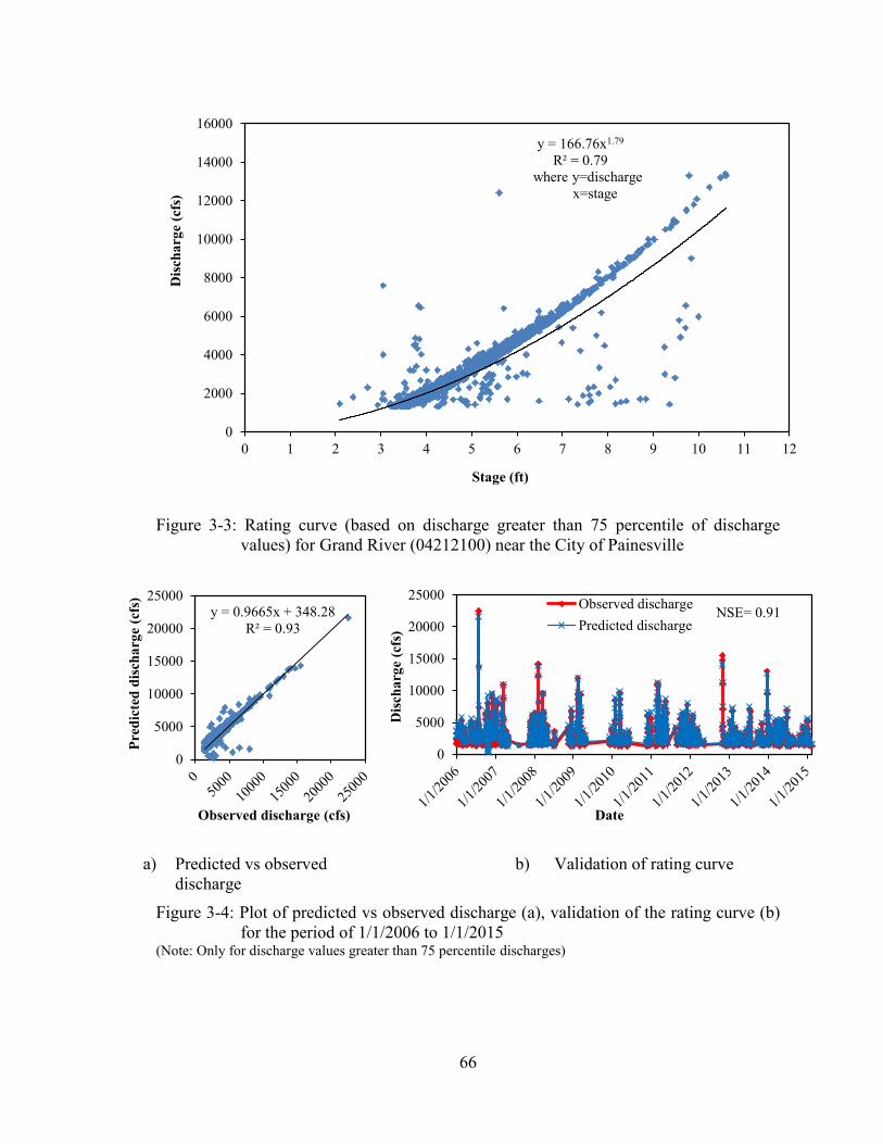
66
Figure 3-3: Rating curve (based on discharge greater than 75 percentile of discharge values) for Grand River (04212100) near the City of Painesville
a) Predicted vs observed discharge
b) Validation of rating curve
Figure 3-4: Plot of predicted vs observed discharge (a), validation of the rating curve (b) for the period of 1/1/2006 to 1/1/2015
(Note: Only for discharge values greater than 75 percentile discharges)
y = 166.76x1.79 R² = 0.79
where y=discharge x=stage
0
2000
4000
6000
8000
10000
12000
14000
16000
0 1 2 3 4 5 6 7 8 9 10 11 12
Dis
char
ge (c
fs)
Stage (ft)
y = 0.9665x + 348.28 R² = 0.93
0
5000
10000
15000
20000
25000
Pred
icte
d di
scha
rge
(cfs
)
Observed discharge (cfs)
0
5000
10000
15000
20000
25000
Dis
char
ge (c
fs)
Date
Observed dischargePredicted discharge
NSE= 0.91
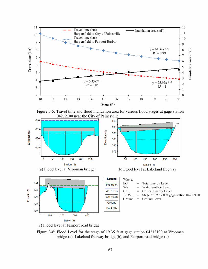
67
Figure 3-5: Travel time and flood inundation area for various flood stages at gage station
04212100 near the City of Painesville
(a) Flood level at Vrooman bridge
(b) Flood level at Lakeland freeway
(c) Flood level at Fairport road bridge
Figure 3-6: Flood Level for the stage of 19.35 ft at gage station 04212100 at Vrooman bridge (a), Lakeland freeway bridge (b), and Fairport road bridge (c)
y = 25.97x-0.60 R² = 1
y = 0.33x0.87 R² = 0.95
y = 64.54x-0.77 R² = 0.99
0
1
2
3
4
5
6
7
8
9
10
11
12
2
3
4
5
6
7
8
9
10
11
10 11 12 13 14 15 16 17 18 19 20 21
Inun
datio
n ar
ea (m
i2 )
Tra
vel t
ime
(hrs
)
Stage (ft)
Where, EG = Total Energy Level WS = Water Surface Level Crit = Critical Energy Level 19.35 = Stage of 19.35 ft at gage station 04212100 Ground = Ground Level
Travel time (hrs) Harpersfield to City of Painesville Travel time (hrs) Harpersfield to Fairport Harbor
Inundation area (mi2)
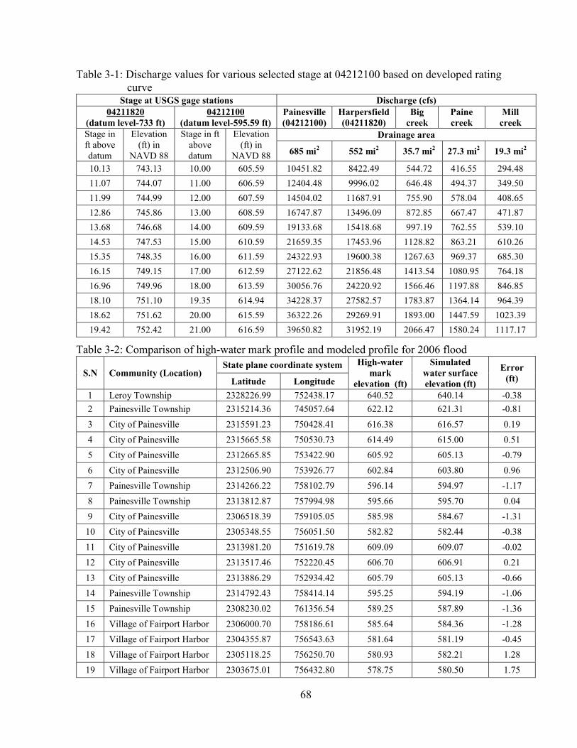
68
Table 3-1: Discharge values for various selected stage at 04212100 based on developed rating curve
Stage at USGS gage stations Discharge (cfs) 04211820
(datum level-733 ft) 04212100
(datum level-595.59 ft) Painesville (04212100)
Harpersfield (04211820)
Big creek
Paine creek
Mill creek
Stage in ft above datum
Elevation (ft) in
NAVD 88
Stage in ft above datum
Elevation (ft) in
NAVD 88
Drainage area
685 mi2 552 mi2 35.7 mi2 27.3 mi2 19.3 mi2
10.13 743.13 10.00 605.59 10451.82 8422.49 544.72 416.55 294.48 11.07 744.07 11.00 606.59 12404.48 9996.02 646.48 494.37 349.50 11.99 744.99 12.00 607.59 14504.02 11687.91 755.90 578.04 408.65 12.86 745.86 13.00 608.59 16747.87 13496.09 872.85 667.47 471.87 13.68 746.68 14.00 609.59 19133.68 15418.68 997.19 762.55 539.10 14.53 747.53 15.00 610.59 21659.35 17453.96 1128.82 863.21 610.26 15.35 748.35 16.00 611.59 24322.93 19600.38 1267.63 969.37 685.30 16.15 749.15 17.00 612.59 27122.62 21856.48 1413.54 1080.95 764.18 16.96 749.96 18.00 613.59 30056.76 24220.92 1566.46 1197.88 846.85 18.10 751.10 19.35 614.94 34228.37 27582.57 1783.87 1364.14 964.39 18.62 751.62 20.00 615.59 36322.26 29269.91 1893.00 1447.59 1023.39 19.42 752.42 21.00 616.59 39650.82 31952.19 2066.47 1580.24 1117.17
Table 3-2: Comparison of high-water mark profile and modeled profile for 2006 flood
S.N Community (Location) State plane coordinate system High-water
mark elevation (ft)
Simulated water surface elevation (ft)
Error (ft) Latitude Longitude
1 Leroy Township 2328226.99 752438.17 640.52 640.14 -0.38 2 Painesville Township 2315214.36 745057.64 622.12 621.31 -0.81 3 City of Painesville 2315591.23 750428.41 616.38 616.57 0.19 4 City of Painesville 2315665.58 750530.73 614.49 615.00 0.51 5 City of Painesville 2312665.85 753422.90 605.92 605.13 -0.79 6 City of Painesville 2312506.90 753926.77 602.84 603.80 0.96 7 Painesville Township 2314266.22 758102.79 596.14 594.97 -1.17 8 Painesville Township 2313812.87 757994.98 595.66 595.70 0.04 9 City of Painesville 2306518.39 759105.05 585.98 584.67 -1.31 10 City of Painesville 2305348.55 756051.50 582.82 582.44 -0.38 11 City of Painesville 2313981.20 751619.78 609.09 609.07 -0.02 12 City of Painesville 2313517.46 752220.45 606.70 606.91 0.21 13 City of Painesville 2313886.29 752934.42 605.79 605.13 -0.66 14 Painesville Township 2314792.43 758414.14 595.25 594.19 -1.06 15 Painesville Township 2308230.02 761356.54 589.25 587.89 -1.36 16 Village of Fairport Harbor 2306000.70 758186.61 585.64 584.36 -1.28 17 Village of Fairport Harbor 2304355.87 756543.63 581.64 581.19 -0.45 18 Village of Fairport Harbor 2305118.25 756250.70 580.93 582.21 1.28 19 Village of Fairport Harbor 2303675.01 756432.80 578.75 580.50 1.75
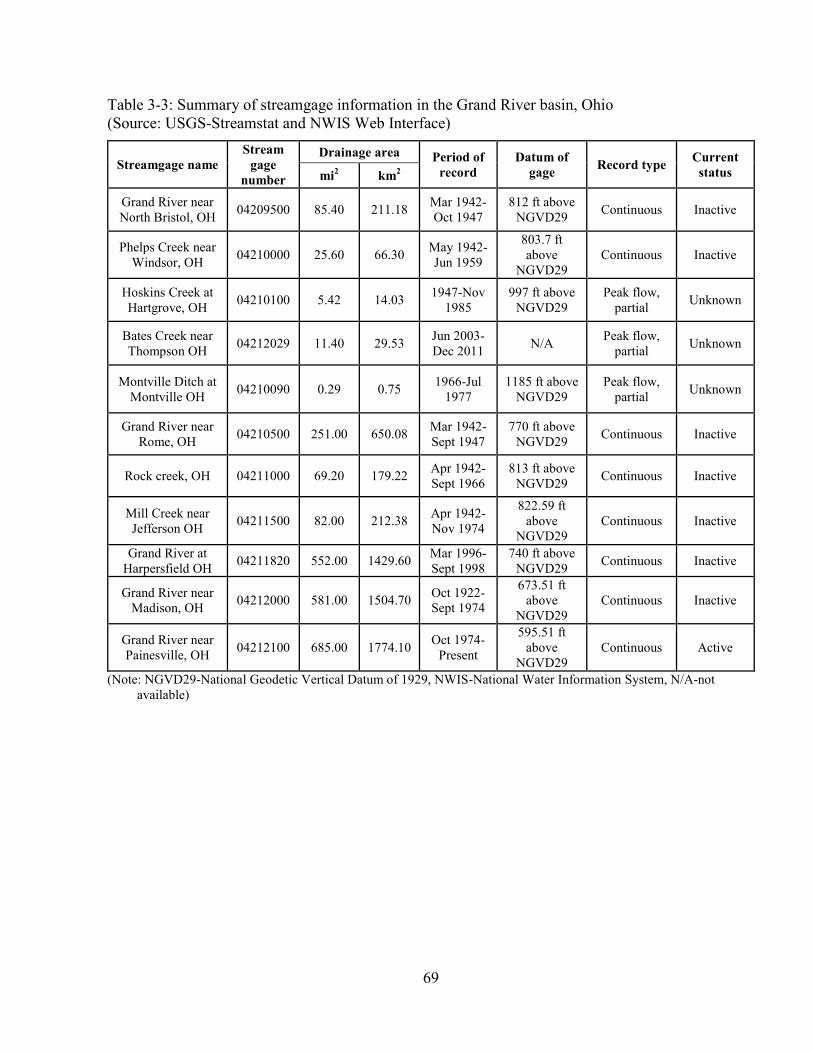
69
Table 3-3: Summary of streamgage information in the Grand River basin, Ohio (Source: USGS-Streamstat and NWIS Web Interface)
Streamgage name Stream
gage number
Drainage area Period of record
Datum of gage Record type Current
status mi2 km2
Grand River near North Bristol, OH 04209500 85.40 211.18 Mar 1942-
Oct 1947 812 ft above
NGVD29 Continuous Inactive
Phelps Creek near Windsor, OH 04210000 25.60 66.30 May 1942-
Jun 1959
803.7 ft above
NGVD29 Continuous Inactive
Hoskins Creek at Hartgrove, OH 04210100 5.42 14.03 1947-Nov
1985 997 ft above
NGVD29 Peak flow,
partial Unknown
Bates Creek near Thompson OH 04212029 11.40 29.53 Jun 2003-
Dec 2011 N/A Peak flow, partial Unknown
Montville Ditch at Montville OH 04210090 0.29 0.75 1966-Jul
1977 1185 ft above
NGVD29 Peak flow,
partial Unknown
Grand River near Rome, OH 04210500 251.00 650.08 Mar 1942-
Sept 1947 770 ft above
NGVD29 Continuous Inactive
Rock creek, OH 04211000 69.20 179.22 Apr 1942-Sept 1966
813 ft above NGVD29 Continuous Inactive
Mill Creek near Jefferson OH 04211500 82.00 212.38 Apr 1942-
Nov 1974
822.59 ft above
NGVD29 Continuous Inactive
Grand River at Harpersfield OH 04211820 552.00 1429.60 Mar 1996-
Sept 1998 740 ft above
NGVD29 Continuous Inactive
Grand River near Madison, OH 04212000 581.00 1504.70 Oct 1922-
Sept 1974
673.51 ft above
NGVD29 Continuous Inactive
Grand River near Painesville, OH 04212100 685.00 1774.10 Oct 1974-
Present
595.51 ft above
NGVD29 Continuous Active
(Note: NGVD29-National Geodetic Vertical Datum of 1929, NWIS-National Water Information System, N/A-not available)
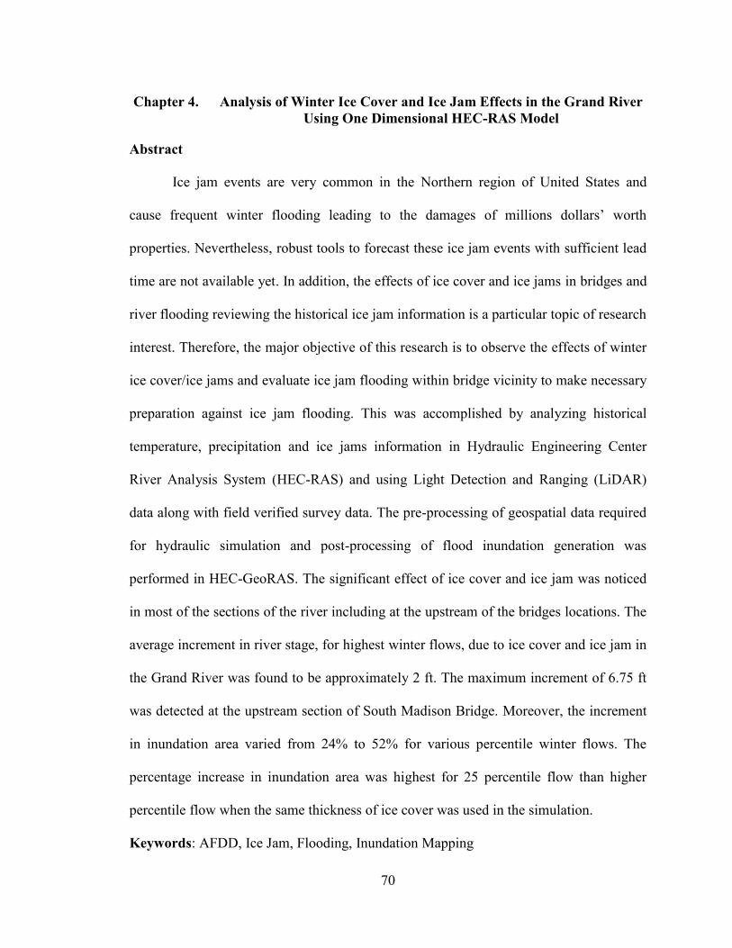
70
Chapter 4. Analysis of Winter Ice Cover and Ice Jam Effects in the Grand River Using One Dimensional HEC-RAS Model
Abstract
Ice jam events are very common in the Northern region of United States and
cause frequent winter flooding leading to the damages of millions dollars’ worth
properties. Nevertheless, robust tools to forecast these ice jam events with sufficient lead
time are not available yet. In addition, the effects of ice cover and ice jams in bridges and
river flooding reviewing the historical ice jam information is a particular topic of research
interest. Therefore, the major objective of this research is to observe the effects of winter
ice cover/ice jams and evaluate ice jam flooding within bridge vicinity to make necessary
preparation against ice jam flooding. This was accomplished by analyzing historical
temperature, precipitation and ice jams information in Hydraulic Engineering Center
River Analysis System (HEC-RAS) and using Light Detection and Ranging (LiDAR)
data along with field verified survey data. The pre-processing of geospatial data required
for hydraulic simulation and post-processing of flood inundation generation was
performed in HEC-GeoRAS. The significant effect of ice cover and ice jam was noticed
in most of the sections of the river including at the upstream of the bridges locations. The
average increment in river stage, for highest winter flows, due to ice cover and ice jam in
the Grand River was found to be approximately 2 ft. The maximum increment of 6.75 ft
was detected at the upstream section of South Madison Bridge. Moreover, the increment
in inundation area varied from 24% to 52% for various percentile winter flows. The
percentage increase in inundation area was highest for 25 percentile flow than higher
percentile flow when the same thickness of ice cover was used in the simulation.
Keywords: AFDD, Ice Jam, Flooding, Inundation Mapping
71
Introduction
River ice processes have significant effects in river hydrology and hydraulics
during the winter time especially in cold regions (Hicks and Beltaos, 2008). Ice jams
processes might lead to the extreme flood events and serious impacts on transportation
and energy production (Prowse et al., 2002). The annual losses due to ice jam have been
estimated to 100 to 135 million USD (Mahabir et al., 2006; White et al., 2007a) in United
States alone, which includes potential losses of human lives, property, structural and
environment damages. Furthermore, ice jam and its movement can severely erode river
beds and banks resulting into adverse effects on aquatic lives (White, K.D., 1999).
Ice jam related flooding is one of the major problems during winter in Northern
region of the United States. Therefore, this study was conducted in the Grand River, near
the City of Painesville where ice jams have frequently occurred in the past at various
locations (USACE, 2015). Most of the jams are occurred in the month of February, while
some occurred in late January, and the rest in early March. These ice jams had led to
closure of many roads and flooding of many properties in the past along the river. There
was an extension of ice jam about a mile between the Richmond and St. Clair St. Bridges
in 1978. Consequently, 150 people from Fairport harbor were evacuated and the
estimated damage of 1.52 million USD was reported. Also, from the historical analysis of
average freezing degree days (AFDD), the highest ice was formed in 1977/1989 period.
Therefore, it is necessary to study the probable effects of ice jam flooding and generate
flood inundation maps separately for winter season to protect human lives and reduce
property damages. Appropriate representation of such flood hazards in this region can be
accomplished by preparing flood maps for winter season as flood maps represent the
72
spatial variability of hazard and provide direct and robust understanding of flood extents
(Merz et al., 2007; Leedal et al., 2010).
Ice jam is a situation of accumulation of fragmented or frazil ice that restricts the
river flow (IAHR, 1986). Flooding is often frequently associated with ice jam in winter
time as ice jam can lead to sudden increase in river stage, which can be much higher
compared to open-water events (Ashton, 1986; White, 2003). Dynamic ice break up
events lead to the greatest variation in river discharge and stage with time (Ferrick et al.,
1992). Sudden increase in river stage and velocities are the result of ice break up events
with a possibility to impose risk to houses, societies and aquatic lives in the downstream
side of the river (Beltaos and Burrell, 2005). Also, there are several effects especially on
bridge structures when the breakup event occurs due to higher river flow, velocities and
hydrodynamic forces during breakup time (Beltaos et al., 2007). Although the discharge
during the ice jam events is lower than that of the open water flow, the stage might
become higher than the stage in open water flow (Lindenschmidt, 2015). Ultimately, this
might bring the situation of potential disaster with socio-economic and environmental
effects (Beltaos, 2011; Carlson, 1989; Brown et al., 2001). However, robust scientific
tool is still not available at present that could be used to forecast the possible future
flooding due to ice jams in advance (Mahavir et al. 2002). More importantly, it is
challenging to predict the location and time of ice jam events as ice jam events are
spatially variable, dependent on river discharge, hydraulics and river geo-morphology
(Wuebben, J. L et al., 1995). Nevertheless, the probable future effects of ice jams can be
found out by modeling the historical ice jam events because if an ice event occurs at the
same location in the future, the database of pre-developed inundation maps can provide
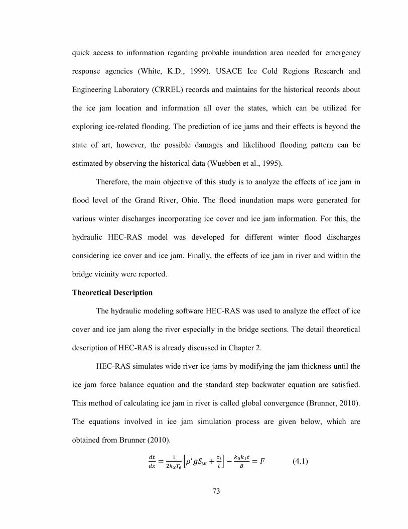
73
quick access to information regarding probable inundation area needed for emergency
response agencies (White, K.D., 1999). USACE Ice Cold Regions Research and
Engineering Laboratory (CRREL) records and maintains for the historical records about
the ice jam location and information all over the states, which can be utilized for
exploring ice-related flooding. The prediction of ice jams and their effects is beyond the
state of art, however, the possible damages and likelihood flooding pattern can be
estimated by observing the historical data (Wuebben et al., 1995).
Therefore, the main objective of this study is to analyze the effects of ice jam in
flood level of the Grand River, Ohio. The flood inundation maps were generated for
various winter discharges incorporating ice cover and ice jam information. For this, the
hydraulic HEC-RAS model was developed for different winter flood discharges
considering ice cover and ice jam. Finally, the effects of ice jam in river and within the
bridge vicinity were reported.
Theoretical Description
The hydraulic modeling software HEC-RAS was used to analyze the effect of ice
cover and ice jam along the river especially in the bridge sections. The detail theoretical
description of HEC-RAS is already discussed in Chapter 2.
HEC-RAS simulates wide river ice jams by modifying the jam thickness until the
ice jam force balance equation and the standard step backwater equation are satisfied.
This method of calculating ice jam in river is called global convergence (Brunner, 2010).
The equations involved in ice jam simulation process are given below, which are
obtained from Brunner (2010).
𝑑𝑡
𝑑𝑥=
1
2𝑘𝑥𝛶𝑒[𝜌′𝑔𝑆𝑤 +
𝜏𝑖
𝑡] −
𝑘0𝑘1𝑡
𝐵= 𝐹 (4.1)
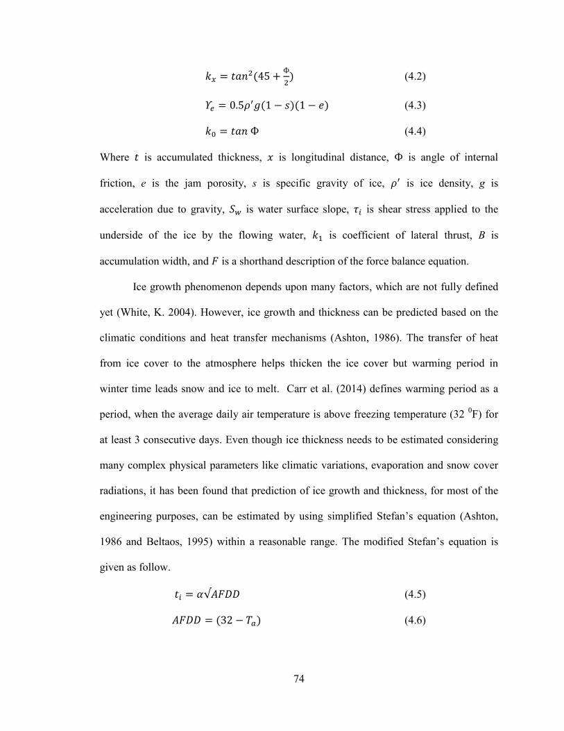
74
𝑘𝑥 = 𝑡𝑎𝑛2(45 +Ф
2) (4.2)
𝛶𝑒 = 0.5𝜌′𝑔(1 − 𝑠)(1 − 𝑒) (4.3)
𝑘0 = 𝑡𝑎𝑛 Ф (4.4)
Where 𝑡 is accumulated thickness, 𝑥 is longitudinal distance, Ф is angle of internal
friction, e is the jam porosity, s is specific gravity of ice, 𝜌′ is ice density, g is
acceleration due to gravity, 𝑆𝑤 is water surface slope, 𝜏𝑖 is shear stress applied to the
underside of the ice by the flowing water, 𝑘1 is coefficient of lateral thrust, B is
accumulation width, and 𝐹 is a shorthand description of the force balance equation.
Ice growth phenomenon depends upon many factors, which are not fully defined
yet (White, K. 2004). However, ice growth and thickness can be predicted based on the
climatic conditions and heat transfer mechanisms (Ashton, 1986). The transfer of heat
from ice cover to the atmosphere helps thicken the ice cover but warming period in
winter time leads snow and ice to melt. Carr et al. (2014) defines warming period as a
period, when the average daily air temperature is above freezing temperature (32 0F) for
at least 3 consecutive days. Even though ice thickness needs to be estimated considering
many complex physical parameters like climatic variations, evaporation and snow cover
radiations, it has been found that prediction of ice growth and thickness, for most of the
engineering purposes, can be estimated by using simplified Stefan’s equation (Ashton,
1986 and Beltaos, 1995) within a reasonable range. The modified Stefan’s equation is
given as follow.
𝑡𝑖 = 𝛼√𝐴𝐹𝐷𝐷 (4.5)
𝐴𝐹𝐷𝐷 = (32 − 𝑇𝑎) (4.6)
75
Where, ti is height of ice cover thickness in inches, α is a coefficient for wind exposure
and snow cover, AFDD is Accumulated Freezing Degree Days and Ta is the daily average
air temperature in 0F.
AFDD is a term that provides an index of winter severity (Carr et al., 2014) and is
calculated using the equation (4.6). The value 0.3 is typically used for α for small
sheltered river. The values of coefficient “α” for different environmental conditions are
listed in Table 4-2. It is worthwhile to note that its application is limited to calculate the
ice thickness at the point of maximum annual AFDD (White, K. 2004). Beyond the point
of peak AFDD, when thawing days start and ice starts to melt, these values of
coefficients are not feasible to estimate the ice thickness (Bilello, 1980). Thawing degree
days (TDD) is basically defined as negative freezing degree-days, which are taken as an
indicator of ice thickness and rate of snowmelt (White et al., 2006).
The ice thickness at the downstream portion is typically calculated based on the
user given upstream ice thickness (Brunner, 2010). The equations to calculate
downstream ice thickness are given below.
𝑡𝑑𝑠 = 𝑡𝑢𝑠 + �̅�𝐿 (4.7)
�̅� =𝐹𝑢𝑠+𝐹𝑑𝑠
2 (4.8)
Where 𝑡𝑑𝑠 𝑖𝑠 thickness at downstream section, 𝑡𝑢𝑠 is thickness at upstream section and L
is the distance between sections. Similarly, 𝐹𝑑𝑠 and 𝐹𝑢𝑠 are ice jam forces at downstream
and upstream sections, respectively. The detail theoretical description of this
phenomenon can be found in Brunner (2010).
The estimation of Manning’s roughness values for the Grand River covered with a
single layer of sheet ice was taken from the recommended values given by White (1999)
76
and Brunner (2010). The channel roughness value at a place where ice jam occurs
depends on total depth of flowing water (Brunner, 2010). The roughness value is
normally calculated using empirical relationship given by Nezhikovsky’s (1964) as
follows.
𝑛𝑖 = 0.0690𝐻−0.23𝑡𝑖0.40 for 𝑡𝑖>1.5 ft (4.9)
𝑛𝑖 = 0.0593𝐻−0.23𝑡𝑖0.77 for 𝑡𝑖<1.5 ft (4.10)
Where 𝑛𝑖 is Manning’s roughness value during ice jam, H is total water depth and 𝑡𝑖 is
the accumulated ice thickness.
Materials and Methodology
Study Area
The study was conducted in Grand River, which is located in Northeastern region
of Ohio. The study area has been described in details in Chapter 2. Grand River has been
frequently threatened by winter flooding due to ice jam in several sections along the
river. The locations of occurrence of ice jam in the Grand River are presented in Figure
4-1 and the other details of ice jam are presented in Table 4-1.
Overall Modeling Approach
The HEC-RAS was used to study the effect of ice jam in the Grand River. Ice
covered channel can be modeled in HEC-RAS by providing the ice thickness and ice jam
information. However, the locations of jams have to be provided manually as HEC-RAS
cannot identify the locations of ice jam in the river (Brunner, 2010). The detail
description of overall modeling approach about model setup and its approach is described
in Chapter 2 under heading “Overall Modeling Approach”. Ice jam modeling approach in
HEC-RAS is described in the following section.
77
At first, the AFDD was calculated for winter period of each year starting from
1949 to 2013. In the next step, the AFDD was used in modified Stefan’s equation to
estimate ice thickness. The maximum possible thickness of ice cover in the Grand River
based on the historical data was selected for the hydraulic analysis. The estimation of
Manning’s roughness values for the Grand River covered with a single layer of sheet ice
was taken from the recommended values given by White (1999) and Brunner (2010). The
adopted value was 0.025. Furthermore, the hydraulic roughness of an ice jam was also
calculated independently using Nezhikovsky’s (1964) equation to provide the value in the
sections where ice jam scenario was applied. The calculated Manning’s roughness value
for various ice jam places varied from 0.022 to 0.025 and the value of 0.025 was adopted.
This was consistent with the adopted value by Wuebben and Gagnon (1995) to model ice
jam flooding on the Missouri River, North Dakota. Since HEC-RAS simulation require
separate set of manning’s roughness for channel/flood plain and ice cover, the roughness
values for river topography was adopted as 0.035 for channel sections and 0.15 for
floodplains as discussed in Chapter 2. The estimated ice thickness was provided for each
cross section in HEC-RAS model in order to model ice jams and evaluate its impact. The
steady state HEC-RAS model was run for three difference scenarios: (a) simulation
without ice cover and jam with bridges; (b) simulation with ice cover and ice jam with
bridges; (c) simulation with ice cover and ice jam but without bridges. The ice jam
locations were chosen based on the historical ice jam along the Grand River. The water
surface elevation at the bridge sections was compared for three different simulation
scenarios using five different discharge values. Similarly, separate flood inundation maps
78
were generated for three different scenarios to observe the difference in inundation areas
due to ice jam especially in bridge locations.
HEC-GeoRAS/HEC-RAS Model Input
All types of data including elevation, streamflow/stage, land cover, bridge, and
lake elevation data have been already described in Chapter 2 under heading “HEC-
GeoRAS/HEC-RAS Model Input”. Temperature data required to calculate AFDD were
downloaded from NOAA-NCDC. Other data required for ice jam simulation like internal
friction angle of jam, ice jam porosity, coefficient of lateral thrust (k1), maximum mean
velocity under ice cover, ice cohesion were adopted from the default values provided in
HEC-RAS (Table 4-3). The ice thickness data needed for ice jam simulation in HEC-
RAS was calculated using modified Stefan’s equation. The steady flow data for winter
simulation were obtained from the historical records. The historical winter discharge
recorded in USGS was analyzed with different percentile values, which are presented in
Table 4-4.
Model Calibration and Validation
The calibration and validation of Manning’s roughness for river channel and flood
plain has been described in detail under heading “Model Calibration and Validation” in
Chapter 2.
Since there were no quantitative data of ice jam thickness for the Grand River, the
model could not be calibrated for ice jam simulation. While the objective of the study
was to make a comparison in water surface level with and without ice cover/ice jam, the
calibration of the model would have little or no effect at all. Therefore, the comparative
79
studies in different flow scenarios were performed, and possible affected regions due to
ice jam flooding were computed for three different scenarios.
Model Evaluation Criteria
The model performance for unsteady flow case was assessed using widely used
statistical parameters such as NSE, R2, PBIAS, and RSR as discussed in Chapter 2.
Results and Discussions
Simulation of Hydraulic Model
The performance of the model was found to be satisfactory in calibration and
validation for different time periods of 1996-1998, which was evaluated based on the
statistical criteria and visual inspection methods as discussed in Chapter 2. However, the
model was not calibrated particularly for winter simulation considering the ice cover and
ice jam scenario due to the lack of quantitative data for ice jam thickness.
AFDD and Ice Thickness Calculation
Since AFDD is the accumulation of freezing degree days, it increases as the
temperature decreases. The maximum AFDD of 1068 degree days was encountered for
1977/1978 (Figure 4-2) based on the analysis of historical data for the period of 1949 to
2013. The ice thickness was estimated using modified Stefan’s equation for winter
periods for the entire period from 1949 to 2013. The value of coefficient “𝛼” in modified
Stefan’s equation was adopted as 0.3. Since, ice thickness is directly proportional to
AFDD, the estimated thickness (10 inches) was also the highest for 1977/1978 period
(Figure 4-2). The maximum value of ice thickness was used to simulate winter discharge
in HEC-RAS to quantify the effect of ice cover and ice jam in river stage and near bridge
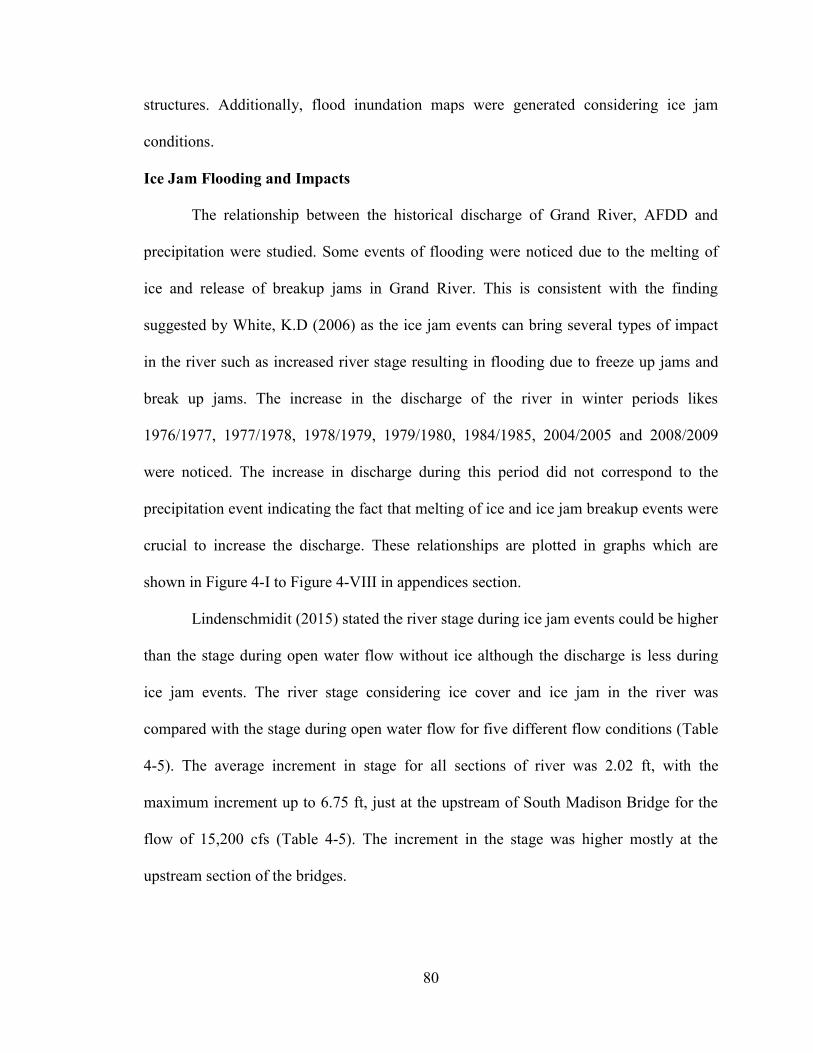
80
structures. Additionally, flood inundation maps were generated considering ice jam
conditions.
Ice Jam Flooding and Impacts
The relationship between the historical discharge of Grand River, AFDD and
precipitation were studied. Some events of flooding were noticed due to the melting of
ice and release of breakup jams in Grand River. This is consistent with the finding
suggested by White, K.D (2006) as the ice jam events can bring several types of impact
in the river such as increased river stage resulting in flooding due to freeze up jams and
break up jams. The increase in the discharge of the river in winter periods likes
1976/1977, 1977/1978, 1978/1979, 1979/1980, 1984/1985, 2004/2005 and 2008/2009
were noticed. The increase in discharge during this period did not correspond to the
precipitation event indicating the fact that melting of ice and ice jam breakup events were
crucial to increase the discharge. These relationships are plotted in graphs which are
shown in Figure 4-I to Figure 4-VIII in appendices section.
Lindenschmidit (2015) stated the river stage during ice jam events could be higher
than the stage during open water flow without ice although the discharge is less during
ice jam events. The river stage considering ice cover and ice jam in the river was
compared with the stage during open water flow for five different flow conditions (Table
4-5). The average increment in stage for all sections of river was 2.02 ft, with the
maximum increment up to 6.75 ft, just at the upstream of South Madison Bridge for the
flow of 15,200 cfs (Table 4-5). The increment in the stage was higher mostly at the
upstream section of the bridges.
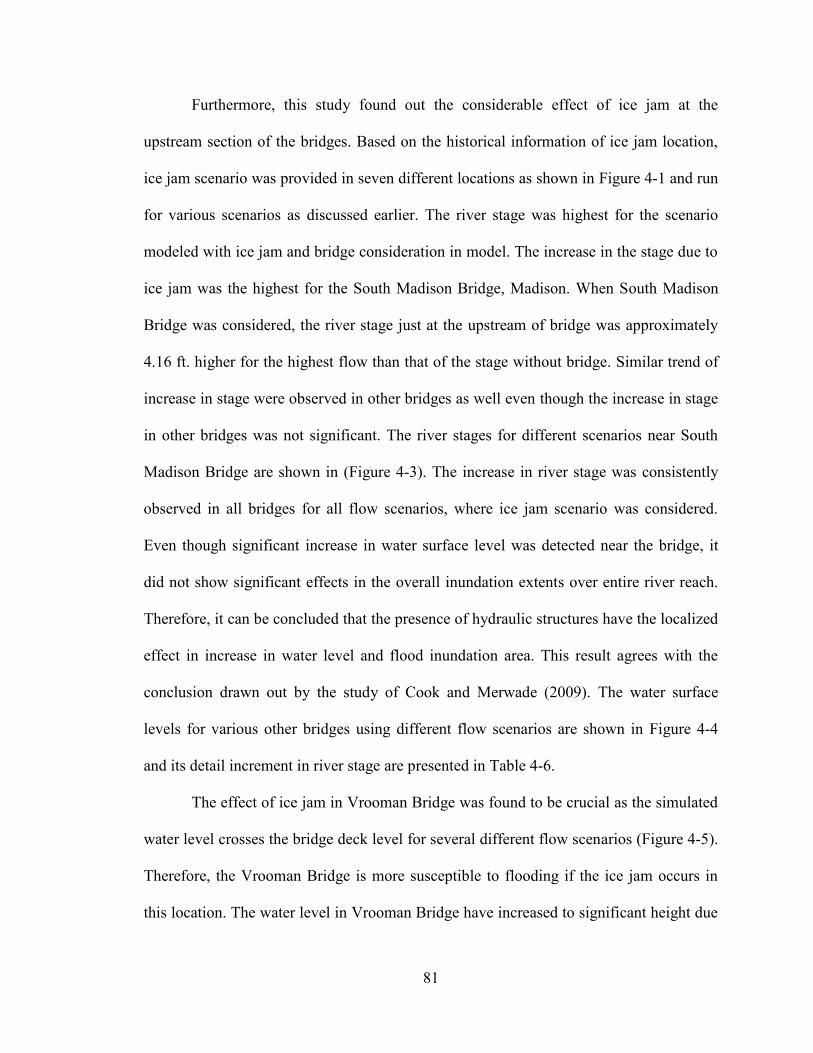
81
Furthermore, this study found out the considerable effect of ice jam at the
upstream section of the bridges. Based on the historical information of ice jam location,
ice jam scenario was provided in seven different locations as shown in Figure 4-1 and run
for various scenarios as discussed earlier. The river stage was highest for the scenario
modeled with ice jam and bridge consideration in model. The increase in the stage due to
ice jam was the highest for the South Madison Bridge, Madison. When South Madison
Bridge was considered, the river stage just at the upstream of bridge was approximately
4.16 ft. higher for the highest flow than that of the stage without bridge. Similar trend of
increase in stage were observed in other bridges as well even though the increase in stage
in other bridges was not significant. The river stages for different scenarios near South
Madison Bridge are shown in (Figure 4-3). The increase in river stage was consistently
observed in all bridges for all flow scenarios, where ice jam scenario was considered.
Even though significant increase in water surface level was detected near the bridge, it
did not show significant effects in the overall inundation extents over entire river reach.
Therefore, it can be concluded that the presence of hydraulic structures have the localized
effect in increase in water level and flood inundation area. This result agrees with the
conclusion drawn out by the study of Cook and Merwade (2009). The water surface
levels for various other bridges using different flow scenarios are shown in Figure 4-4
and its detail increment in river stage are presented in Table 4-6.
The effect of ice jam in Vrooman Bridge was found to be crucial as the simulated
water level crosses the bridge deck level for several different flow scenarios (Figure 4-5).
Therefore, the Vrooman Bridge is more susceptible to flooding if the ice jam occurs in
this location. The water level in Vrooman Bridge have increased to significant height due
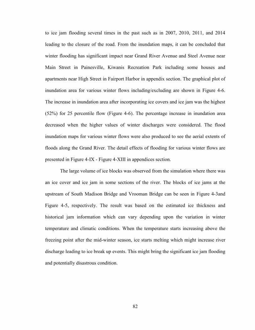
82
to ice jam flooding several times in the past such as in 2007, 2010, 2011, and 2014
leading to the closure of the road. From the inundation maps, it can be concluded that
winter flooding has significant impact near Grand River Avenue and Steel Avenue near
Main Street in Painesville, Kiwanis Recreation Park including some houses and
apartments near High Street in Fairport Harbor in appendix section. The graphical plot of
inundation area for various winter flows including/excluding are shown in Figure 4-6.
The increase in inundation area after incorporating ice covers and ice jam was the highest
(52%) for 25 percentile flow (Figure 4-6). The percentage increase in inundation area
decreased when the higher values of winter discharges were considered. The flood
inundation maps for various winter flows were also produced to see the aerial extents of
floods along the Grand River. The detail effects of flooding for various winter flows are
presented in Figure 4-IX - Figure 4-XIII in appendices section.
The large volume of ice blocks was observed from the simulation where there was
an ice cover and ice jam in some sections of the river. The blocks of ice jams at the
upstream of South Madison Bridge and Vrooman Bridge can be seen in Figure 4-3and
Figure 4-5, respectively. The result was based on the estimated ice thickness and
historical jam information which can vary depending upon the variation in winter
temperature and climatic conditions. When the temperature starts increasing above the
freezing point after the mid-winter season, ice starts melting which might increase river
discharge leading to ice break up events. This might bring the significant ice jam flooding
and potentially disastrous condition.
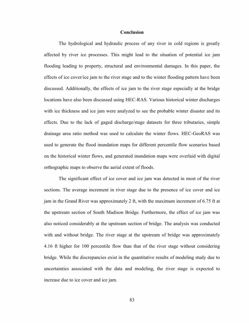
83
Conclusion
The hydrological and hydraulic process of any river in cold regions is greatly
affected by river ice processes. This might lead to the situation of potential ice jam
flooding leading to property, structural and environmental damages. In this paper, the
effects of ice cover/ice jam to the river stage and to the winter flooding pattern have been
discussed. Additionally, the effects of ice jam to the river stage especially at the bridge
locations have also been discussed using HEC-RAS. Various historical winter discharges
with ice thickness and ice jam were analyzed to see the probable winter disaster and its
effects. Due to the lack of gaged discharge/stage datasets for three tributaries, simple
drainage area ratio method was used to calculate the winter flows. HEC-GeoRAS was
used to generate the flood inundation maps for different percentile flow scenarios based
on the historical winter flows, and generated inundation maps were overlaid with digital
orthographic maps to observe the aerial extent of floods.
The significant effect of ice cover and ice jam was detected in most of the river
sections. The average increment in river stage due to the presence of ice cover and ice
jam in the Grand River was approximately 2 ft, with the maximum increment of 6.75 ft at
the upstream section of South Madison Bridge. Furthermore, the effect of ice jam was
also noticed considerably at the upstream section of bridge. The analysis was conducted
with and without bridge. The river stage at the upstream of bridge was approximately
4.16 ft higher for 100 percentile flow than that of the river stage without considering
bridge. While the discrepancies exist in the quantitative results of modeling study due to
uncertainties associated with the data and modeling, the river stage is expected to
increase due to ice cover and ice jam.
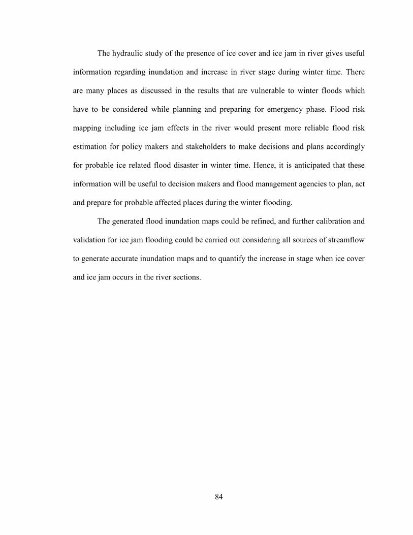
84
The hydraulic study of the presence of ice cover and ice jam in river gives useful
information regarding inundation and increase in river stage during winter time. There
are many places as discussed in the results that are vulnerable to winter floods which
have to be considered while planning and preparing for emergency phase. Flood risk
mapping including ice jam effects in the river would present more reliable flood risk
estimation for policy makers and stakeholders to make decisions and plans accordingly
for probable ice related flood disaster in winter time. Hence, it is anticipated that these
information will be useful to decision makers and flood management agencies to plan, act
and prepare for probable affected places during the winter flooding.
The generated flood inundation maps could be refined, and further calibration and
validation for ice jam flooding could be carried out considering all sources of streamflow
to generate accurate inundation maps and to quantify the increase in stage when ice cover
and ice jam occurs in the river sections.
85
References
Ashton, G. D. (Ed.). (1986). River and lake ice engineering. Water Resources
Publication.
Ashton, G. D. "Ice jam flooding on the Peace River near the Peace Athabasca
Delta." Water Stewardship: How Are We Managing (2003): 11-13.
Beltaos, Spyros, ed. River ice jams. Water Resources Publication, 1995.
Beltaos, S. (2011). Alternative method for synthetic frequency analysis of breakup jam
floods. CGU HS Committee on river ice processes and environment, 18-22.
Beltaos, S., & Prowse, T. D. (2001). Climate impacts on extreme ice-jam events in
Canadian rivers. Hydrological Sciences Journal, 46(1), 157-181.
Beltaos, Spyros, and Brian C. Burrell. "Climatic change and river ice breakup." Canadian
Journal of Civil Engineering 30.1 (2003): 145-155.
Brunner, Gary W. HEC-RAS River Analysis System. Hydraulic Reference Manual.
Version 4.1. HYDROLOGIC ENGINEERING CENTER DAVIS CA, 2010.
Beltaos, Spyros, et al. "Hydraulic effects of ice breakup on bridges."Canadian Journal of
Civil Engineering 34.4 (2007): 539-548.
Bilello, M. A. (1980). Maximum thickness and subsequent decay of lake, river and fast
sea ice in Canada and Alaska (No. CRREL-80-6). COLD REGIONS RESEARCH
AND ENGINEERING LAB HANOVER NH.
Brown, R. S., G. Power, and S. Beltaoa. "Winter movements and habitat use of riverine
brown trout, white sucker and common carp in relation to flooding and ice
break‐ up." Journal of Fish Biology 59.5 (2001): 1126-1141.
Beltaos, Spyros, and Brian C. Burrell. "Field measurements of ice-jam-release
surges." Canadian Journal of Civil Engineering 32.4 (2005): 699-711.
Carr, Meredith L., and Carrie M. Vuyovich. "Investigating the effects of long-term
hydro-climatic trends on Midwest ice jam events." Cold Regions Science and
Technology 106 (2014): 66-81.
86
Carlson, Robert F., John P. Zarling, and Lewis E. Link. "Cold Regions Engineering
Research-Strategic Plan." Journal of Cold Regions Engineering3.4 (1989): 172-
190.
Ferrick, Michael G., Patricia B. Weyrick, and Susan T. Hunnewell. "Analysis of river ice
motion near a breaking front." Canadian Journal of Civil Engineering 19.1 (1992):
105-116.
Hicks, Faye, and Spyros Beltaos. "River ice." Cold Region Atmospheric and Hydrologic
Studies. The Mackenzie GEWEX Experience. Springer Berlin Heidelberg, 2008.
281-305.
IAHR, 1986. River ice jams: a state of the art report, working group on river ice
hydraulics. Proceedings of the International Association for Hydraulics Research
International Symposium on Ice. , vol 3, pp. 561–594 (Iowa City, IA).
Lindenschmidt, Karl-Erich, et al. "Ice jam flood hazard assessment and mapping of the
Peace River at the Town of Peace River." 2015
Mahabir, C., Hicks, F. E., & Fayek, A. R. (2002, December). Forecasting ice jam risk at
Fort McMurray, AB using fuzzy logic. In Proceedings of the 16th IAHR
International Symposium on Ice, International Association of Hydraulic
Engineering and Research, New Zealand, 2nd–6th December (pp. 91-98).
Mahabir, Chandra, Faye Hicks, and Aminah Robinson Fayek. "Neuro-fuzzy river ice
breakup forecasting system." Cold regions science and technology 46.2 (2006):
100-112.
Merz, Bruno, A. H. Thieken, and Martin Gocht. "Flood risk mapping at the local scale:
concepts and challenges." Flood risk management in Europe. Springer
Netherlands, 2007. 231-251.
Leedal, David, et al., "Visualization approaches for communicating real-time flood
forecasting level and inundation information." Journal of Flood Risk
Management 3.2 (2010): 140-150.
Prowse, Terry D., and Spyros Beltaos. "Climatic control of river‐ ice hydrology: a
review." Hydrological processes 16.4 (2002): 805-822.
87
USACE, 2015 CRREL Ice Jam Database for gage station 04212100 in Grand River, OH
(accessed March 2015) http://rsgisias.crrel.usace.army.mil/apex/f?p=524:5:0::NO
WHITE, KATHLEEN D., ANDREW M. TUTHILL, and LINNZI FURMAN. "Studies
of ice jam flooding in the United States." Extreme Hydrological Events: New
Concepts for Security. Springer Netherlands, 2006. 255-268.
White, Kathleen D. "Review of prediction methods for breakup ice jams." Canadian
Journal of Civil Engineering 30.1 (2003): 89-100.
White, K.D., Tuthill, A.M., Furman, L., 2007a. Studies of ice jam flooding in the United
States. Extreme Hydrological Events: New Concepts for Security. Springer, Netherlands.
White, Kathleen D. Hydraulic and physical properties affecting ice jams. No. CRREL-
99-11. COLD REGIONS RESEARCH AND ENGINEERING LAB HANOVER
NH, 1999.
White, K. (2004). Method to estimate river ice thickness based on meteorological data:
ERDC. CRREL Technical Note TN-04-3, US Army Engineer Research and
Development Center, Hanover, New Hampshire.
Wuebben, James L., and John J. Gagnon. Ice jam flooding on the Missouri River near
Williston, North Dakota. No. CRREL-95-19. COLD REGIONS RESEARCH
AND ENGINEERING LAB HANOVER NH, 1995.
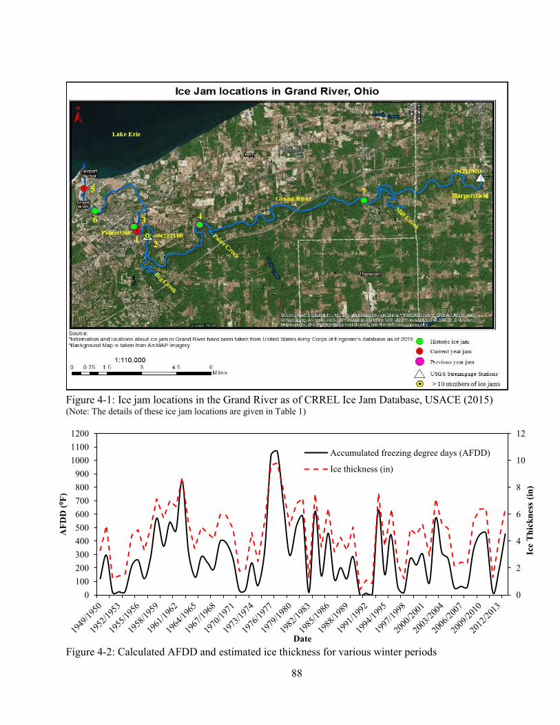
88
Figure 4-1: Ice jam locations in the Grand River as of CRREL Ice Jam Database, USACE (2015) (Note: The details of these ice jam locations are given in Table 1)
Figure 4-2: Calculated AFDD and estimated ice thickness for various winter periods
0
2
4
6
8
10
12
0100200300400500600700800900
100011001200
Ice
Thi
ckne
ss (i
n)
AFD
D (0 F
)
Date
Accumulated freezing degree days (AFDD)
Ice thickness (in)
1
3
2
4
7 5
6
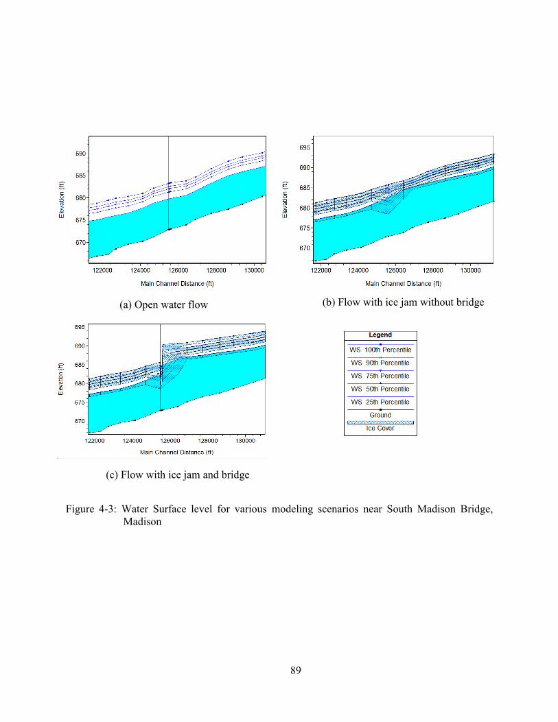
89
Figure 4-3: Water Surface level for various modeling scenarios near South Madison Bridge,
Madison
(a) Open water flow
(b) Flow with ice jam without bridge
(c) Flow with ice jam and bridge
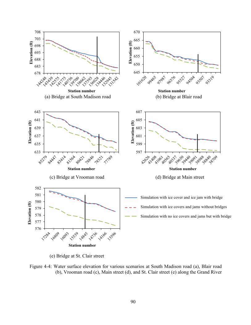
90
(a) Bridge at South Madison road
(b) Bridge at Blair road
(c) Bridge at Vrooman road
(d) Bridge at Main street
(e) Bridge at St. Clair street
Figure 4-4: Water surface elevation for various scenarios at South Madison road (a), Blair road (b), Vrooman road (c), Main street (d), and St. Clair street (e) along the Grand River
678
683
688
693
698
703
708E
leva
tion
(ft)
Station number
645
650
655
660
665
670
Ele
vatio
n (f
t)
Station number
633
635
637
639
641
643
Ele
vatio
n (f
t)
Station number
597
599
601
603
605
607
Ele
vatio
n (f
t)
Station number
576
577
578
579
580
581
582
Ele
vatio
n (f
t)
Station number
Simulation with ice cover and ice jam with bridge
Simulation with ice covers and jams without bridges
Simulation with no ice covers and jams but with bridge
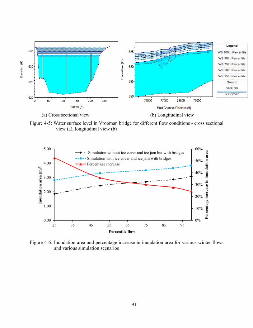
91
(a) Cross sectional view (b) Longitudinal view
Figure 4-5: Water surface level in Vrooman bridge for different flow conditions - cross sectional view (a), longitudinal view (b)
Figure 4-6: Inundation area and percentage increase in inundation area for various winter flows and various simulation scenarios
0%
10%
20%
30%
40%
50%
60%
0.00
1.00
2.00
3.00
4.00
5.00
25 35 45 55 65 75 85 95
Perc
enta
ge in
crea
se in
inun
datio
n ar
ea
Inun
datio
n ar
ea (m
i2 )
Percentile flow
Simulation without ice cover and ice jam but with bridgesSimulation with ice cover and ice jam with bridgesPercentage increase
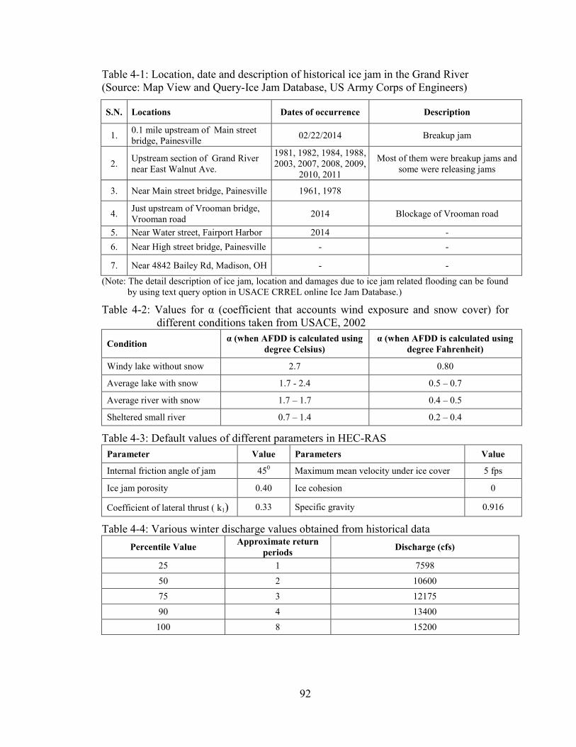
92
Table 4-1: Location, date and description of historical ice jam in the Grand River (Source: Map View and Query-Ice Jam Database, US Army Corps of Engineers)
S.N. Locations Dates of occurrence Description
1. 0.1 mile upstream of Main street bridge, Painesville 02/22/2014 Breakup jam
2. Upstream section of Grand River near East Walnut Ave.
1981, 1982, 1984, 1988, 2003, 2007, 2008, 2009,
2010, 2011
Most of them were breakup jams and some were releasing jams
3. Near Main street bridge, Painesville 1961, 1978
4. Just upstream of Vrooman bridge, Vrooman road 2014 Blockage of Vrooman road
5. Near Water street, Fairport Harbor 2014 - 6. Near High street bridge, Painesville - -
7. Near 4842 Bailey Rd, Madison, OH - -
(Note: The detail description of ice jam, location and damages due to ice jam related flooding can be found by using text query option in USACE CRREL online Ice Jam Database.)
Table 4-2: Values for α (coefficient that accounts wind exposure and snow cover) for different conditions taken from USACE, 2002
Condition α (when AFDD is calculated using degree Celsius)
α (when AFDD is calculated using degree Fahrenheit)
Windy lake without snow 2.7 0.80
Average lake with snow 1.7 - 2.4 0.5 – 0.7
Average river with snow 1.7 – 1.7 0.4 – 0.5
Sheltered small river 0.7 – 1.4 0.2 – 0.4
Table 4-3: Default values of different parameters in HEC-RAS Parameter Value Parameters Value
Internal friction angle of jam 450 Maximum mean velocity under ice cover 5 fps
Ice jam porosity 0.40 Ice cohesion 0
Coefficient of lateral thrust ( k1) 0.33 Specific gravity 0.916
Table 4-4: Various winter discharge values obtained from historical data Percentile Value Approximate return
periods Discharge (cfs)
25 1 7598 50 2 10600 75 3 12175 90 4 13400
100 8 15200
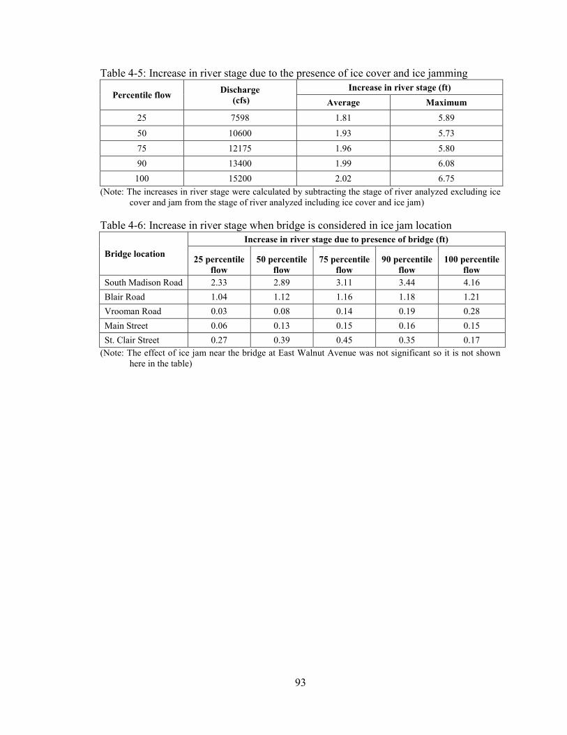
93
Table 4-5: Increase in river stage due to the presence of ice cover and ice jamming
Percentile flow Discharge (cfs)
Increase in river stage (ft) Average Maximum
25 7598 1.81 5.89
50 10600 1.93 5.73 75 12175 1.96 5.80 90 13400 1.99 6.08
100 15200 2.02 6.75 (Note: The increases in river stage were calculated by subtracting the stage of river analyzed excluding ice
cover and jam from the stage of river analyzed including ice cover and ice jam)
Table 4-6: Increase in river stage when bridge is considered in ice jam location
Bridge location Increase in river stage due to presence of bridge (ft)
25 percentile flow
50 percentile flow
75 percentile flow
90 percentile flow
100 percentile flow
South Madison Road 2.33 2.89 3.11 3.44 4.16 Blair Road 1.04 1.12 1.16 1.18 1.21 Vrooman Road 0.03 0.08 0.14 0.19 0.28 Main Street 0.06 0.13 0.15 0.16 0.15 St. Clair Street 0.27 0.39 0.45 0.35 0.17
(Note: The effect of ice jam near the bridge at East Walnut Avenue was not significant so it is not shown here in the table)
94
Chapter 5. Conclusion and Recommendations
In this study, an approach for flood warning system was introduced including
digital map preparation and travel time computation. Furthermore, the effects of
resolutions of elevation datasets and Manning’s roughness in prediction of travel time
and flood inundation areas were investigated. The study utilized a broadly accepted tool,
HEC-RAS to perform the required hydraulic simulation. A HEC-GeoRAS, an ArcGIS
extension, was used to produce flood inundations maps. The hydraulic model was
calibrated and validated with satisfactory model performance for various periods from
1996 to 1998 using USGS discharge and stage data.
The hydraulic model was setup for various return period floods using different elevation
datasets and a range of possible roughness values to observe the uncertainties involved in
flood inundation mapping process. A topographic survey was conducted to get accurate
elevation dataset in the river channel sections. The results obtained from LiDAR
integrated with survey data, were considered the reference datasets to compare the results
obtained using other elevation datasets. The predicted travel time and inundation area
was highest, for the most coarse elevation dataset (30m DEM) without integration of
survey data, and this was in decreasing trend while using finer elevation datasets. Since
the predicted travel time, from 10m DEM without integration of survey data, showed less
percentage difference than LiDAR without survey, it was concluded that elevation data in
channel was better represented by 10m DEM than LiDAR data. However, this does not
rule out the necessity of a topographic survey for accurate elevation datasets. Similarly,
the selection of Manning’s roughness in the channel sections and floodplains were found
to be very important for the prediction of travel time and flood inundation areas.
95
However, the Manning’s roughness value in channel sections was sensitive compared to
the roughness values in floodplains. The maximum decrease in inundation area was
1.49%, when Manning’s roughness was varied in floodplain and kept constant in channel.
Similarly, the decrease in inundation area was 8.97%, when Manning’s roughness was
varied in channel section and kept constant in floodplain. Therefore, it is essential to
consider those discrepancies while predicting flood travel time and generating flood
inundation maps.
Furthermore, rating curve was developed using historical discharge and stage data
to estimate the peak flood discharge for 12 different flood stages ranging from 10.00 ft to
21.00 ft, which were approximately 2 to 500 year return period floods. The digital flood
inundation maps were generated for various flood stages based on the upstream and
downstream gage heights. There are more than 100 houses and apartments, many roads,
bridges and parks along the Grand River, which are vulnerable to 500 years return period
flood within the study area. It is recommended to install the siren system at suitable
locations to issue warning in sufficient time ahead. The predicted flood travel time from
the study can be utilized to evacuate the people from probable inundation area.
The significant effect of ice cover and ice jam was found in most of the sections
of the river during the winter period. There was an increase in river stage when the
simulation was performed considering ice cover and ice jam along the river. Additional
increase in river stage at the upstream section of bridges was found when bridges were
considered in the model simulation. However, the flooding was limited to upstream and
the increase in flooding extents was not realized along the entire river. The average
increase in stage along the entire Grand River within study area was found to be
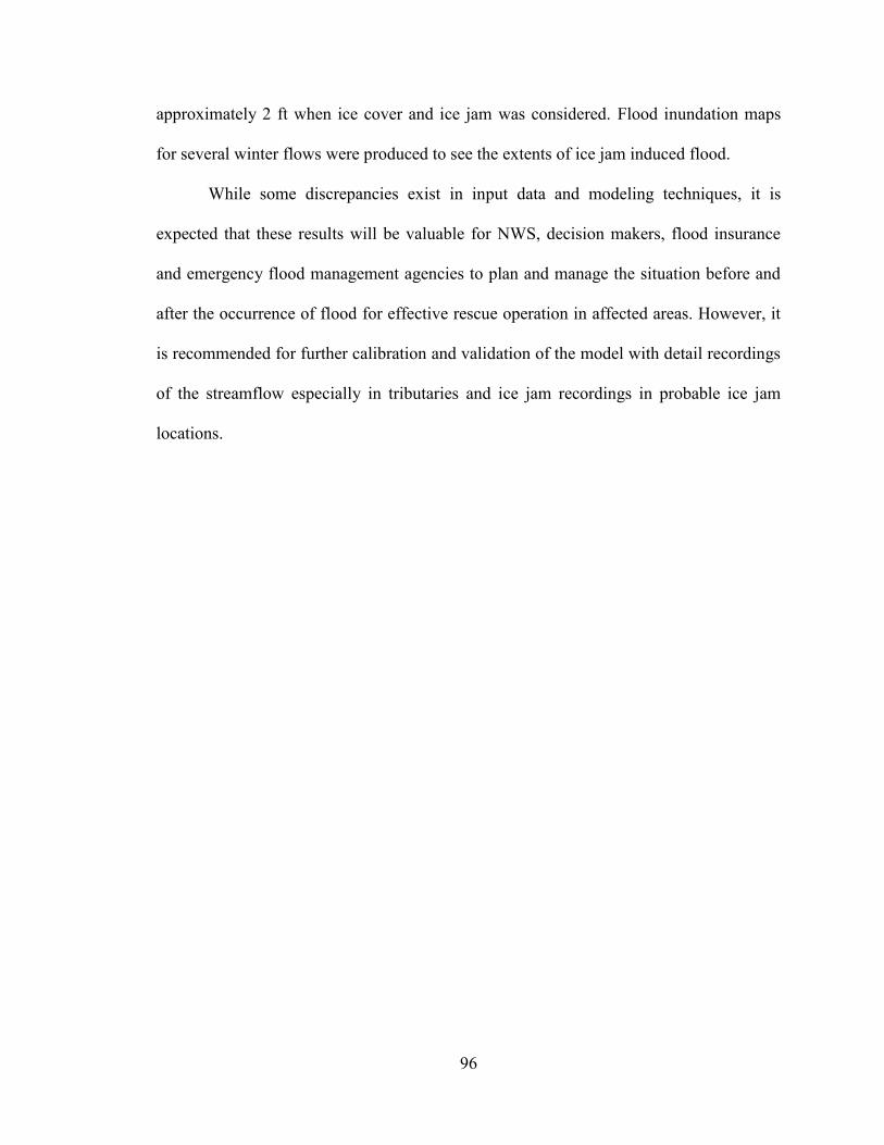
96
approximately 2 ft when ice cover and ice jam was considered. Flood inundation maps
for several winter flows were produced to see the extents of ice jam induced flood.
While some discrepancies exist in input data and modeling techniques, it is
expected that these results will be valuable for NWS, decision makers, flood insurance
and emergency flood management agencies to plan and manage the situation before and
after the occurrence of flood for effective rescue operation in affected areas. However, it
is recommended for further calibration and validation of the model with detail recordings
of the streamflow especially in tributaries and ice jam recordings in probable ice jam
locations.

97
APPENDICES
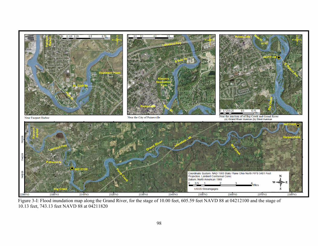
98
Figure 3-I: Flood inundation map along the Grand River, for the stage of 10.00 feet, 605.59 feet NAVD 88 at 04212100 and the stage of 10.13 feet, 743.13 feet NAVD 88 at 04211820
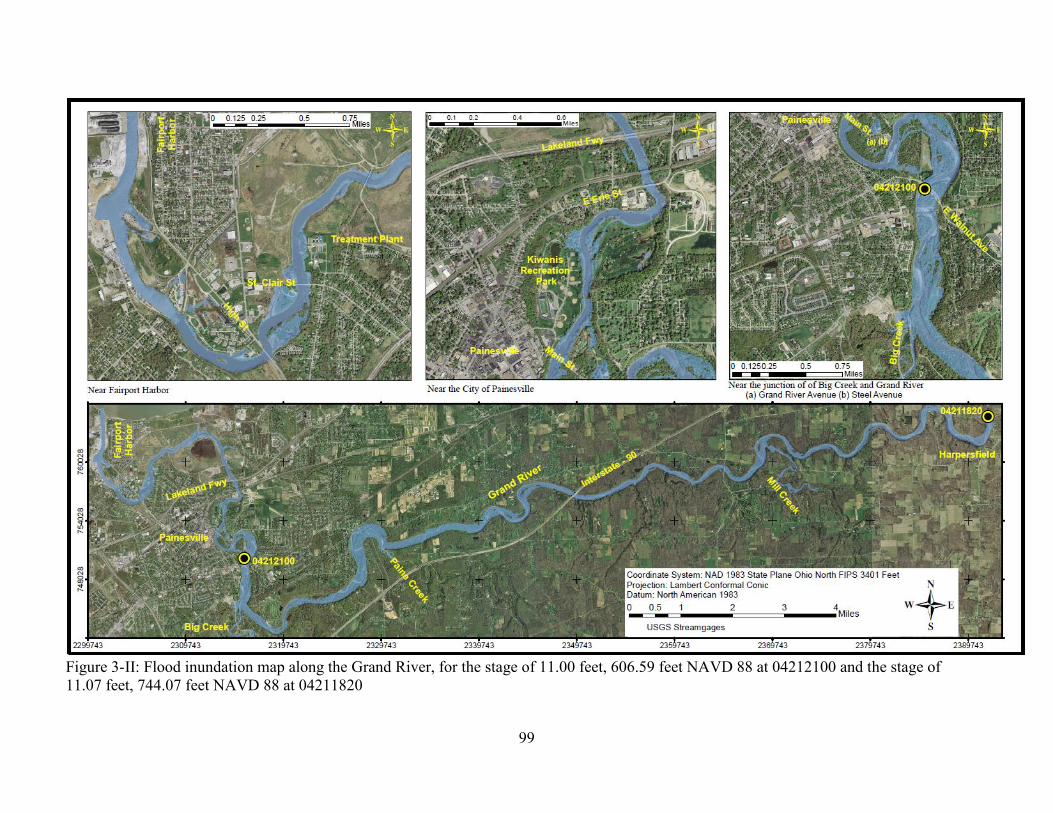
99
Figure 3-II: Flood inundation map along the Grand River, for the stage of 11.00 feet, 606.59 feet NAVD 88 at 04212100 and the stage of 11.07 feet, 744.07 feet NAVD 88 at 04211820

100
Figure 3-III: Flood inundation map along the Grand River, for the stage of 12.00 feet, 607.59 feet NAVD 88 at 04212100 and the stage of 11.99 feet, 744.99 feet NAVD 88 at 04211820
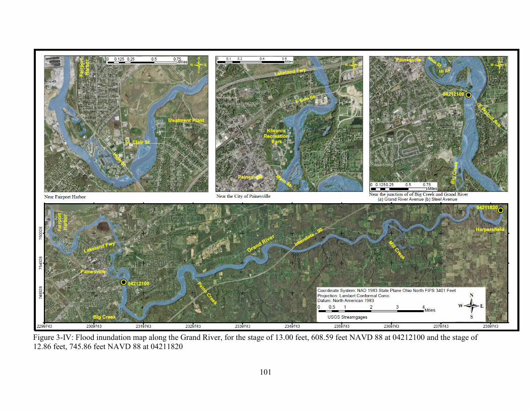
101
Figure 3-IV: Flood inundation map along the Grand River, for the stage of 13.00 feet, 608.59 feet NAVD 88 at 04212100 and the stage of 12.86 feet, 745.86 feet NAVD 88 at 04211820
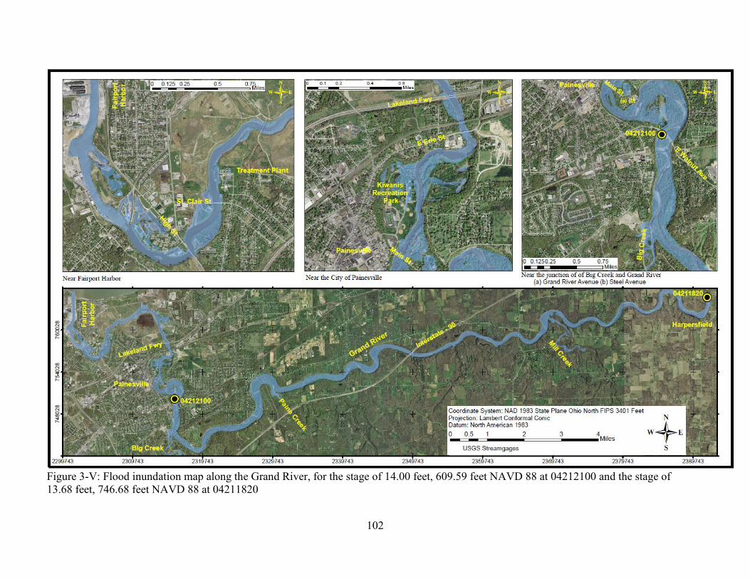
102
Figure 3-V: Flood inundation map along the Grand River, for the stage of 14.00 feet, 609.59 feet NAVD 88 at 04212100 and the stage of 13.68 feet, 746.68 feet NAVD 88 at 04211820
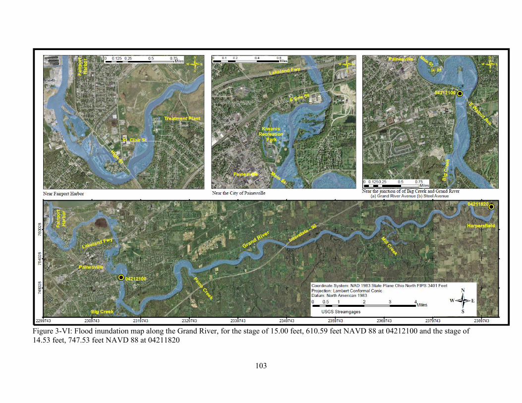
103
Figure 3-VI: Flood inundation map along the Grand River, for the stage of 15.00 feet, 610.59 feet NAVD 88 at 04212100 and the stage of 14.53 feet, 747.53 feet NAVD 88 at 04211820
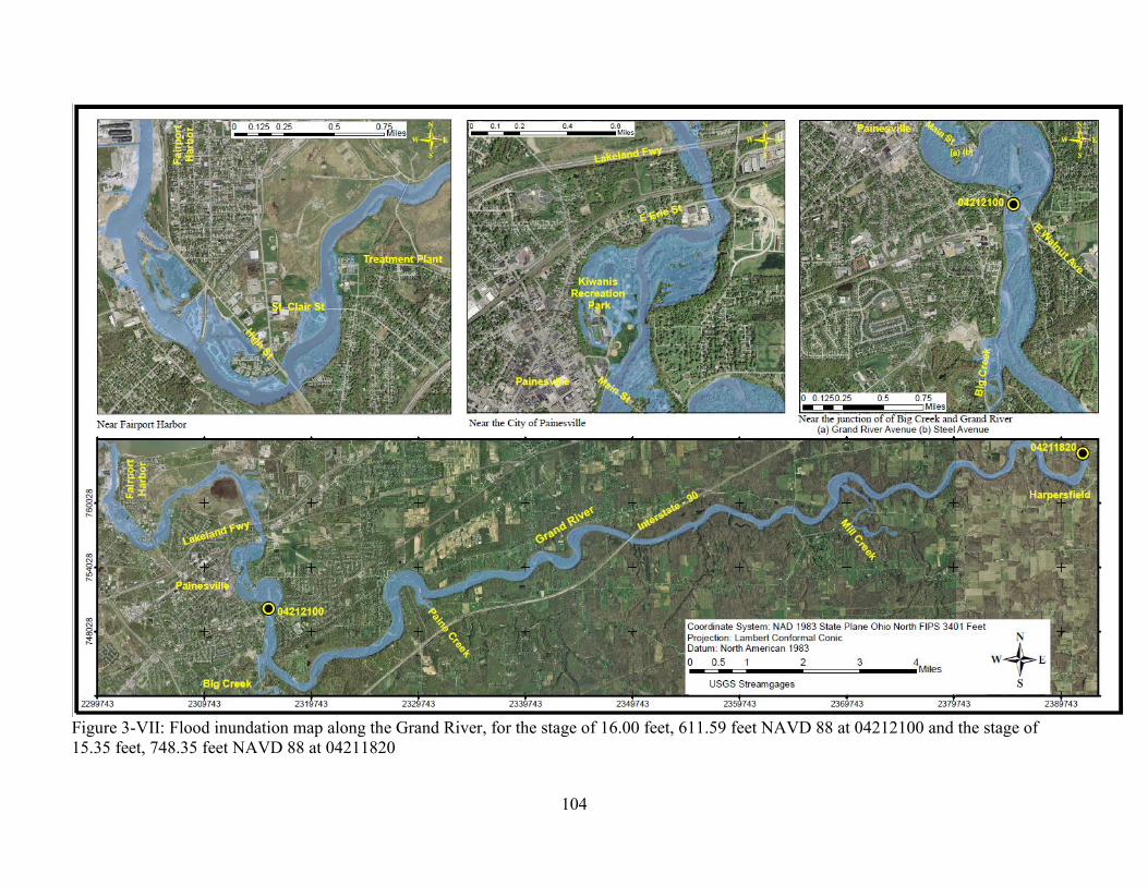
104
Figure 3-VII: Flood inundation map along the Grand River, for the stage of 16.00 feet, 611.59 feet NAVD 88 at 04212100 and the stage of 15.35 feet, 748.35 feet NAVD 88 at 04211820

105
Figure 3-VIII: Flood inundation map along the Grand River, for the stage of 17.00 feet, 612.59 feet NAVD 88 at 04212100 and the stage of 16.15 feet, 749.15 feet NAVD 88 at 04211820
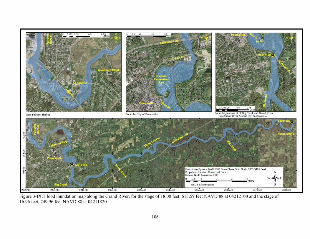
106
Figure 3-IX: Flood inundation map along the Grand River, for the stage of 18.00 feet, 613.59 feet NAVD 88 at 04212100 and the stage of 16.96 feet, 749.96 feet NAVD 88 at 04211820

107
Figure 3-X: Flood inundation map along the Grand River, for the stage of 19.35 feet, 614.94 feet NAVD 88 at 04212100 and the stage of 18.10 feet, 751.10 feet NAVD 88 at 04211820
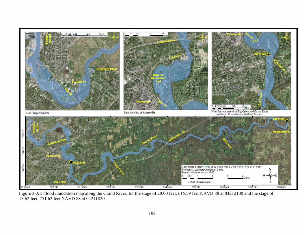
108
Figure 3-XI: Flood inundation map along the Grand River, for the stage of 20.00 feet, 615.59 feet NAVD 88 at 04212100 and the stage of 18.62 feet, 751.62 feet NAVD 88 at 04211820
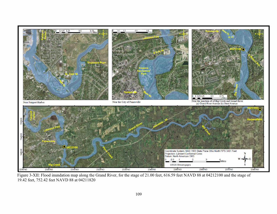
109
Figure 3-XII: Flood inundation map along the Grand River, for the stage of 21.00 feet, 616.59 feet NAVD 88 at 04212100 and the stage of 19.42 feet, 752.42 feet NAVD 88 at 04211820
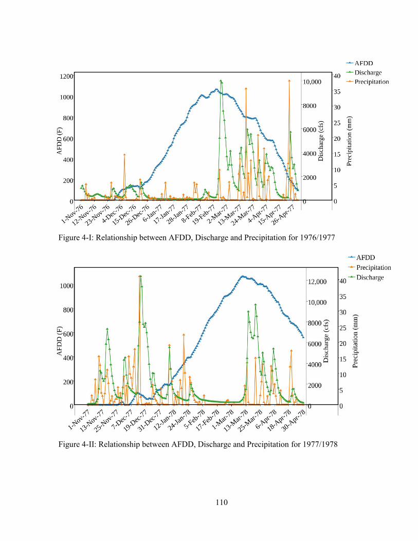
110
Figure 4-I: Relationship between AFDD, Discharge and Precipitation for 1976/1977
Figure 4-II: Relationship between AFDD, Discharge and Precipitation for 1977/1978
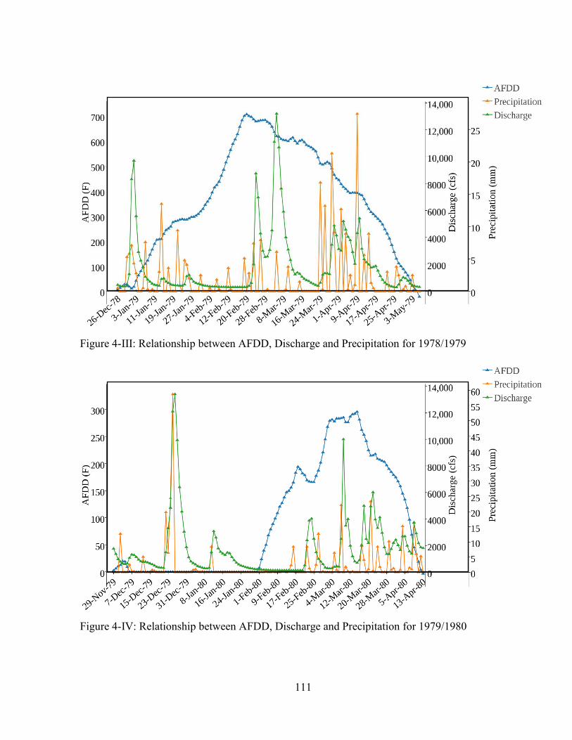
111
Figure 4-III: Relationship between AFDD, Discharge and Precipitation for 1978/1979
Figure 4-IV: Relationship between AFDD, Discharge and Precipitation for 1979/1980
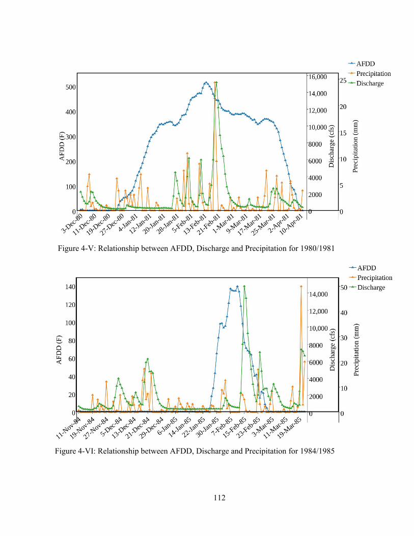
112
Figure 4-V: Relationship between AFDD, Discharge and Precipitation for 1980/1981
Figure 4-VI: Relationship between AFDD, Discharge and Precipitation for 1984/1985
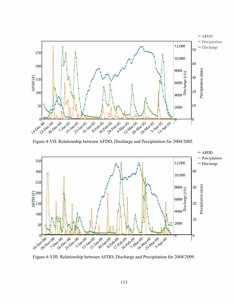
113
Figure 4-VII: Relationship between AFDD, Discharge and Precipitation for 2004/2005
Figure 4-VIII: Relationship between AFDD, Discharge and Precipitation for 2008/2009
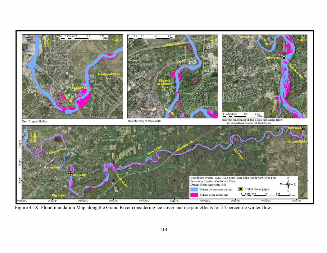
114
Figure 4-IX: Flood inundation Map along the Grand River considering ice cover and ice jam effects for 25 percentile winter flow.
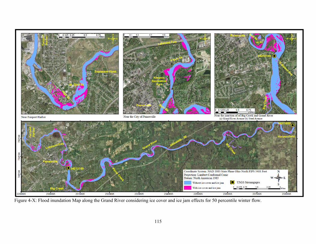
115
Figure 4-X: Flood inundation Map along the Grand River considering ice cover and ice jam effects for 50 percentile winter flow.
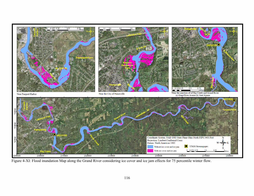
116
Figure 4-XI: Flood inundation Map along the Grand River considering ice cover and ice jam effects for 75 percentile winter flow.
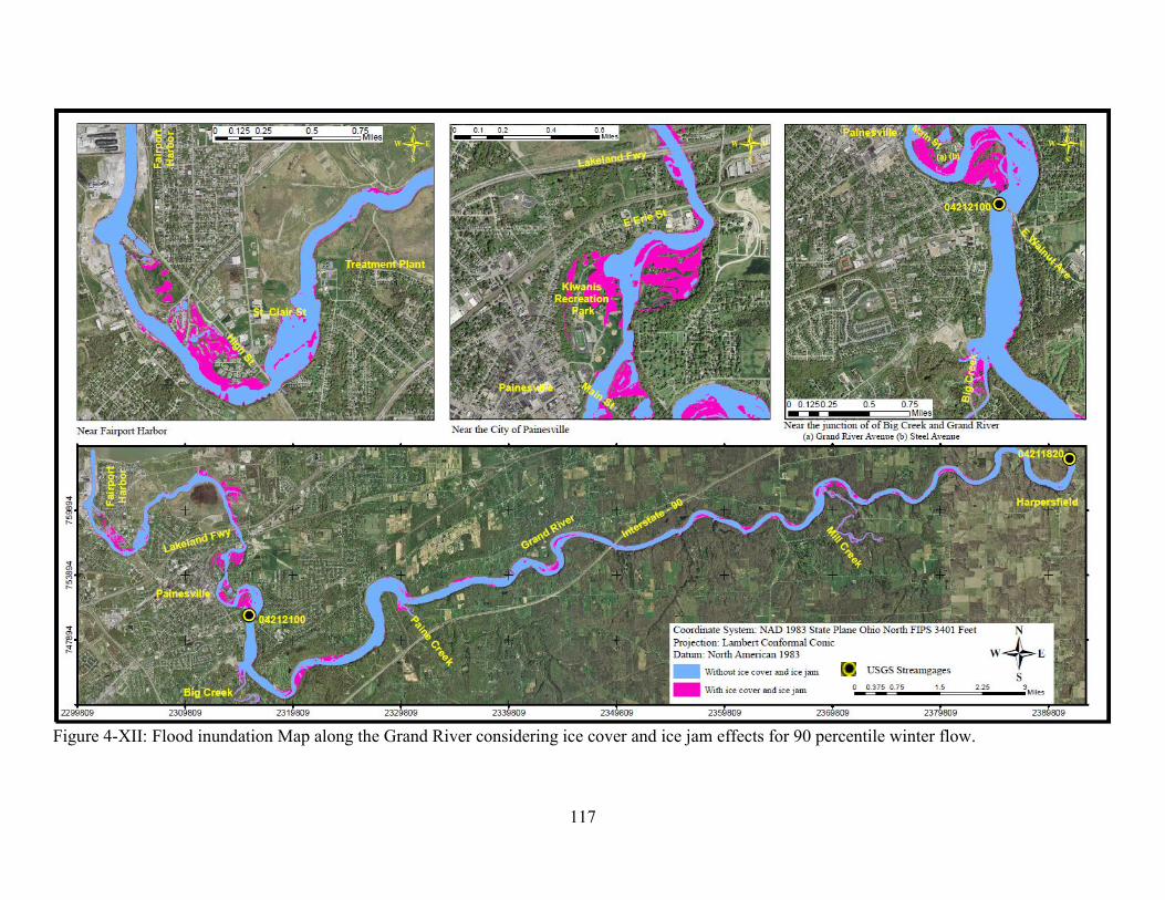
117
Figure 4-XII: Flood inundation Map along the Grand River considering ice cover and ice jam effects for 90 percentile winter flow.
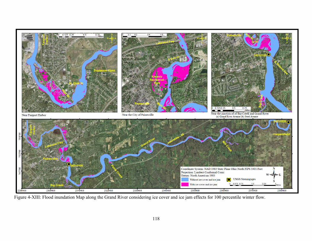
118
Figure 4-XIII: Flood inundation Map along the Grand River considering ice cover and ice jam effects for 100 percentile winter flow.


