
Laser Fundamentals
Electro-Optics & Applications Prof. Elias N. Glytsis
School of Electrical & Computer Engineering National Technical University of Athens
23/01/2019

E1
E2
N1
N2
hν = E2 ‒ E1
E1
E2
N1
N2
hν = E2 ‒ E1
E1
E2
N1
N2
hν = E2 ‒ E1
Radiative Processes
Spontaneous Emission
Absorption
Stimulated Emission
2 Prof. Elias N. Glytsis, School of ECE, NTUA
For Blackbody Radiation:

Prof. Elias N. Glytsis, School of ECE, NTUA 3
L ight A mplification S timulated E mission R adiation
Radiative Processes of Stimulated Emission Basic Principle of laser Operation
http://www.laserfest.org/lasers/images/nero1.jpg
Prof. Elias N. Glytsis, School of ECE, NTUA 4
E1
E2
N1
N2
hν = E2 ‒ E1
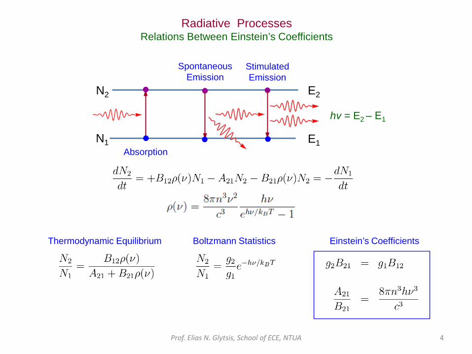
Absorption
Spontaneous Emission
Stimulated Emission
Radiative Processes Relations Between Einstein’s Coefficients
Thermodynamic Equilibrium Boltzmann Statistics Einstein’s Coefficients

Prof. Elias N. Glytsis, School of ECE, NTUA 5
Lineshape Function
E1
E2
N1
N2 hν = E2 ‒ E1
Lineshape Function, g(ν) = Probability g(ν)dν for a photon to be - Spontaneously Emitted between ν and ν+dν - Absorbed between ν and ν+dν - Spontaneously Emitted between ν and ν+dν

Prof. Elias N. Glytsis, School of ECE, NTUA 6
Damped Oscillation
E1
E2
N1
N2 hν = E2 ‒ E1

Prof. Elias N. Glytsis, School of ECE, NTUA 7
Damped Oscillation (He-Ne laser transition λ0 = 0.6328μm)
Prof. Elias N. Glytsis, School of ECE, NTUA 8
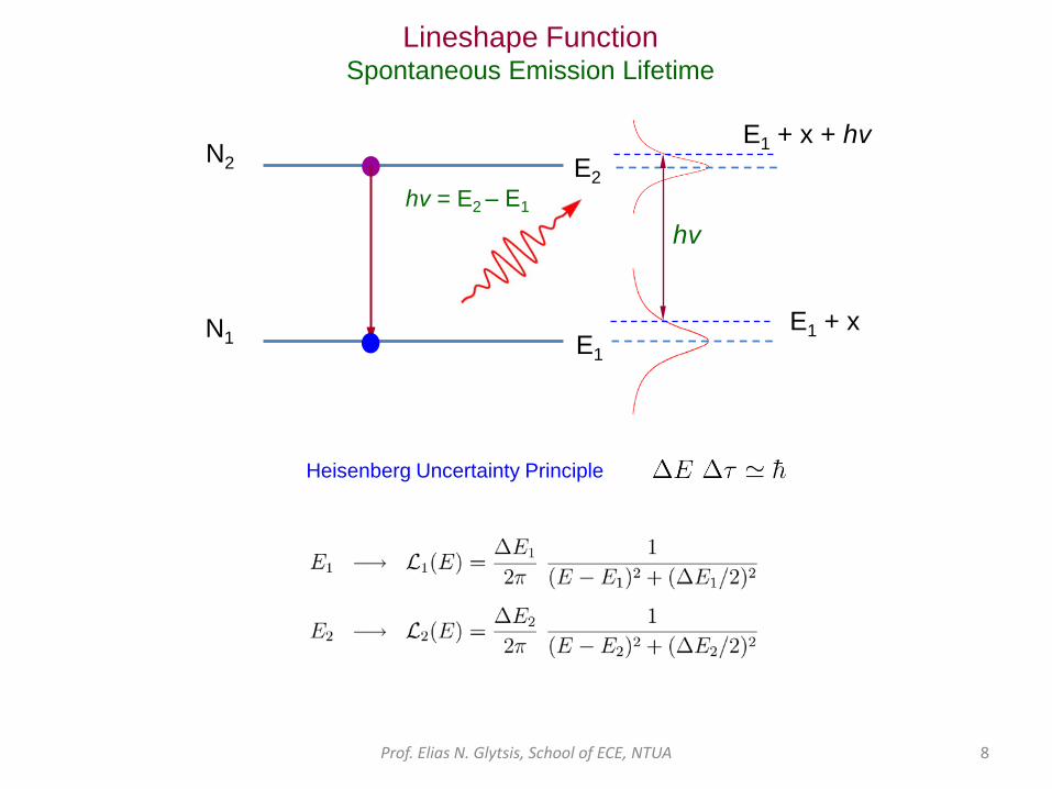
Lineshape Function Spontaneous Emission Lifetime
Heisenberg Uncertainty Principle
E1
E2
N1
N2
hν = E2 ‒ E1 hν
E1 + x
E1 + x + hν
Prof. Elias N. Glytsis, School of ECE, NTUA 9
E1
E2
N1
N2
hν = E2 ‒ E1 hν
E1 + x
E1 + x + hν
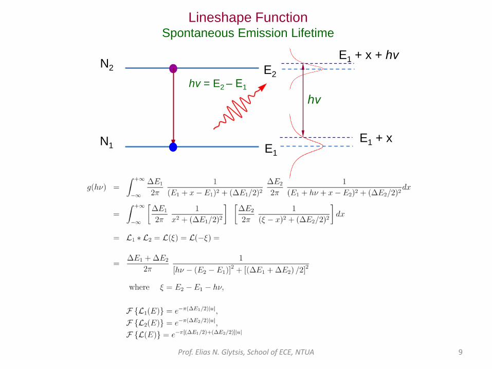
Lineshape Function Spontaneous Emission Lifetime

Prof. Elias N. Glytsis, School of ECE, NTUA 10
Damped Oscillation with Elastic Collisions

Prof. Elias N. Glytsis, School of ECE, NTUA 11
Damped Oscillation with Elastic Collisions
Average over 1000 random events
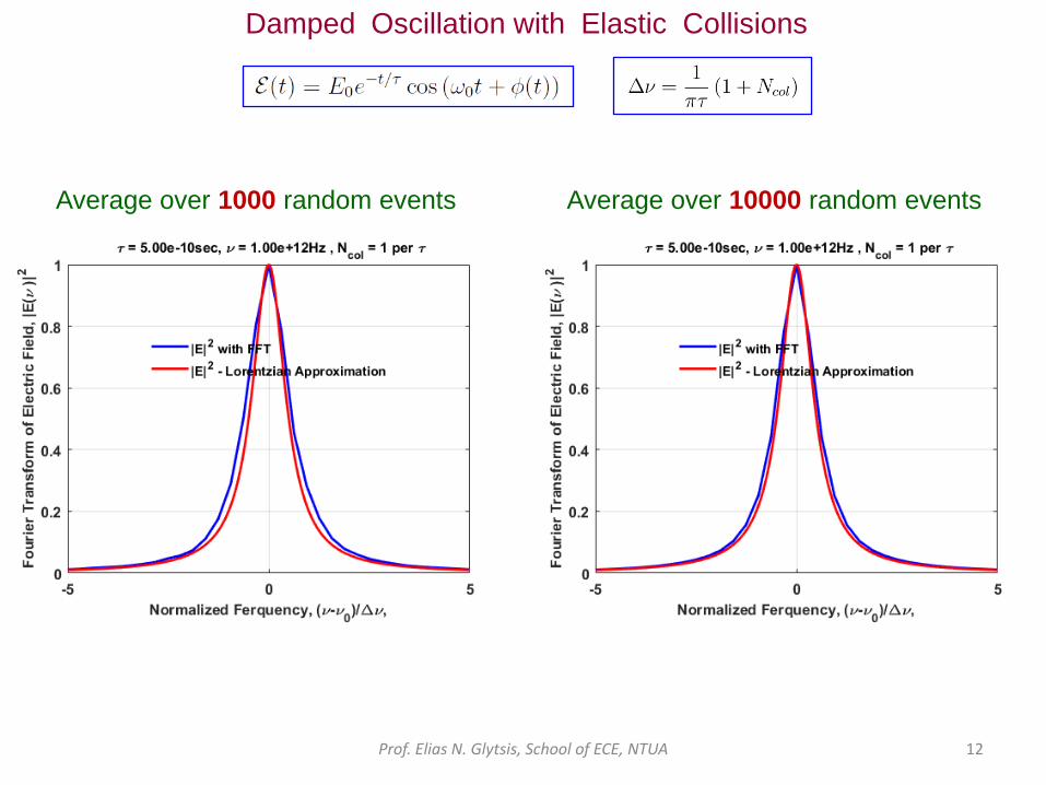
Prof. Elias N. Glytsis, School of ECE, NTUA 12
Damped Oscillation with Elastic Collisions
Average over 1000 random events Average over 10000 random events

Prof. Elias N. Glytsis, School of ECE, NTUA 13
Damped Oscillation with Elastic Collisions
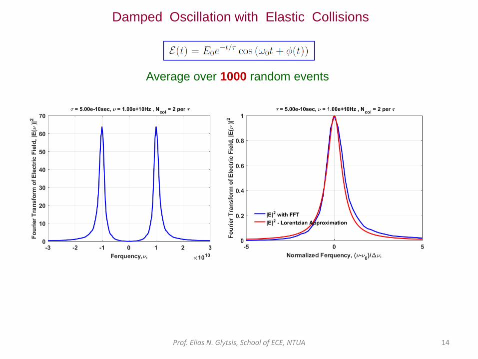
Prof. Elias N. Glytsis, School of ECE, NTUA 14
Damped Oscillation with Elastic Collisions
Average over 1000 random events
Prof. Elias N. Glytsis, School of ECE, NTUA 15
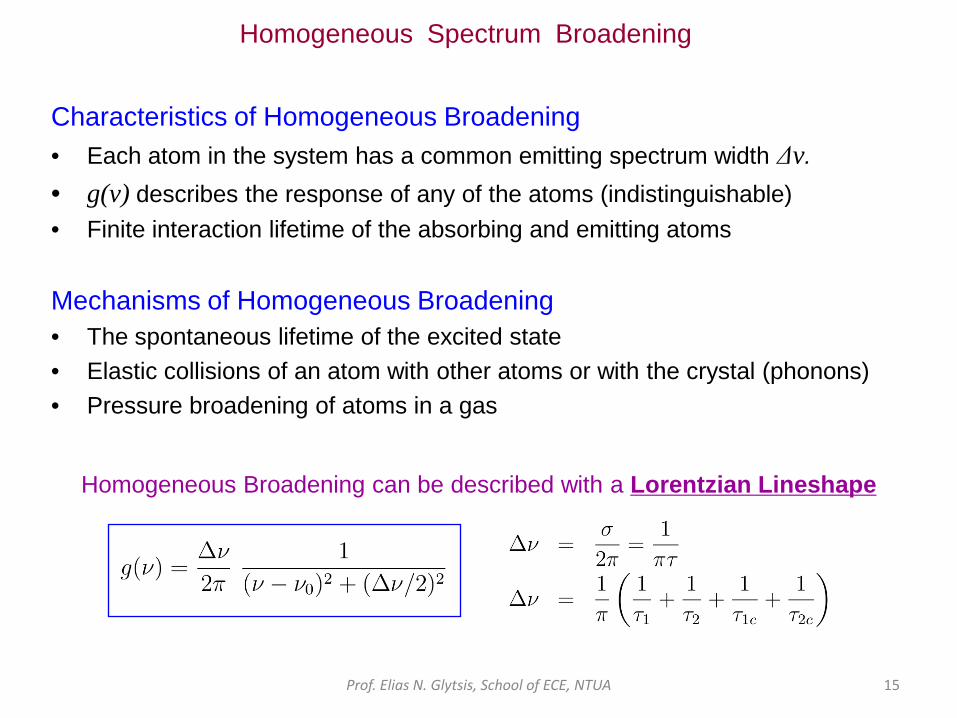
Homogeneous Spectrum Broadening
Characteristics of Homogeneous Broadening • Each atom in the system has a common emitting spectrum width Δv. • g(v) describes the response of any of the atoms (indistinguishable) • Finite interaction lifetime of the absorbing and emitting atoms Mechanisms of Homogeneous Broadening • The spontaneous lifetime of the excited state • Elastic collisions of an atom with other atoms or with the crystal (phonons) • Pressure broadening of atoms in a gas
Homogeneous Broadening can be described with a Lorentzian Lineshape
Prof. Elias N. Glytsis, School of ECE, NTUA 16
Inhomogeneous Spectrum Broadening
Features of Inhomogeneous Broadening • Individual atoms are distinguishable, each having a slightly different
frequency due to “seeing” slightly different environment • The observed spectrum of spontaneous emission reflects the spread in the
individual transition frequencies (not only the broadening due to the finite lifetime of the excited state)
Example Mechanisms of Inhomogeneous Broadening • The energy levels of impurity in a host crystal • Random strain • Crystal imperfections • Doppler effect in gases

Prof. Elias N. Glytsis, School of ECE, NTUA 17
Maxwell-Boltzmann Velocity Distribution

Prof. Elias N. Glytsis, School of ECE, NTUA 18
Maxwell-Boltzmann Velocity Distribution
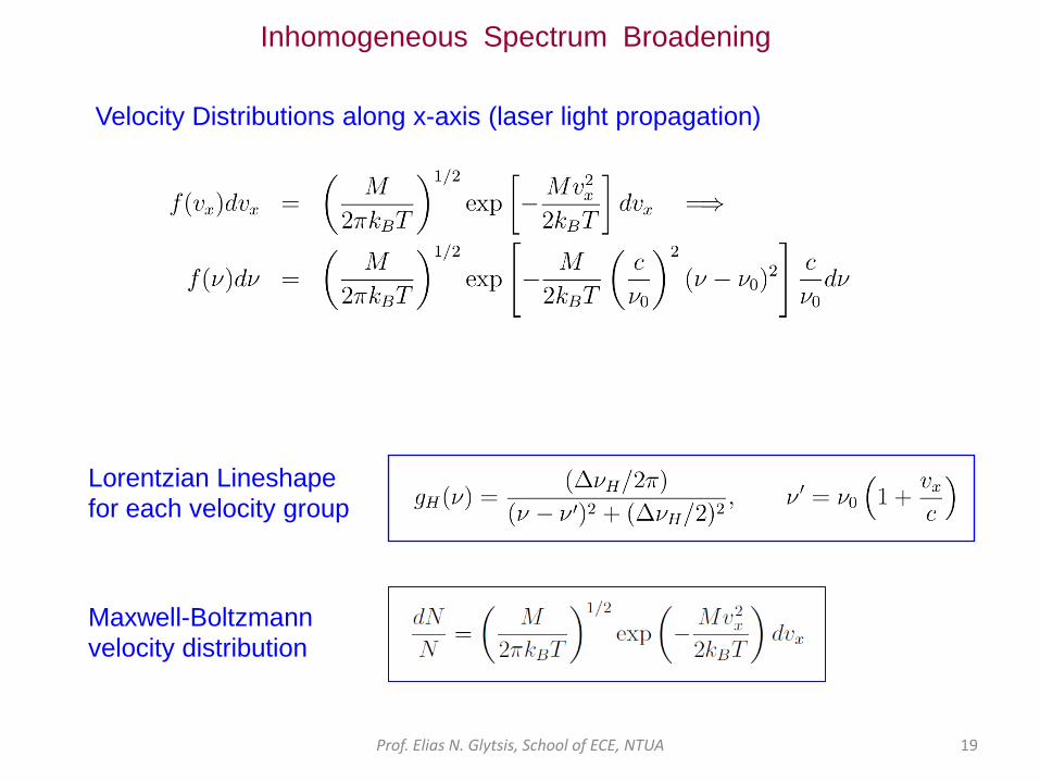
Velocity Distributions along x-axis (laser light propagation)
Doppler Effect
Prof. Elias N. Glytsis, School of ECE, NTUA 19
Inhomogeneous Spectrum Broadening
Maxwell-Boltzmann velocity distribution
Lorentzian Lineshape for each velocity group
Velocity Distributions along x-axis (laser light propagation)

Prof. Elias N. Glytsis, School of ECE, NTUA 20
Inhomogeneous Spectrum Broadening
Average Lineshape Function
Voigt Lineshape Function
F. Schreir, “Optimized implementations of rational approximations for the Voigt and complex error function”, Journal of Quantitative Spectroscopy & Radiative Transfer 112 (2011) 1010–1025
Prof. Elias N. Glytsis, School of ECE, NTUA 21
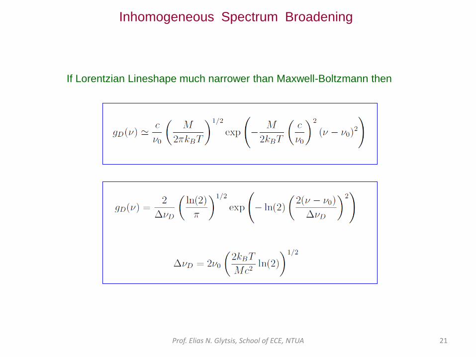
Inhomogeneous Spectrum Broadening
If Lorentzian Lineshape much narrower than Maxwell-Boltzmann then

Prof. Elias N. Glytsis, School of ECE, NTUA 22
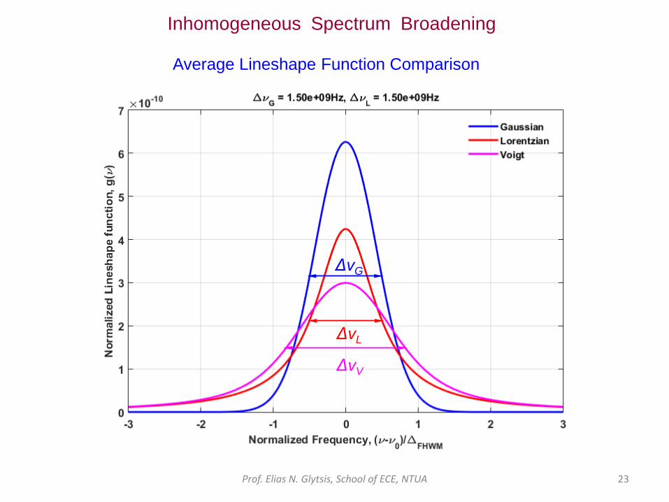
Inhomogeneous Spectrum Broadening
Average Lineshape Function Comparison
ΔνG
ΔνL
Prof. Elias N. Glytsis, School of ECE, NTUA 23
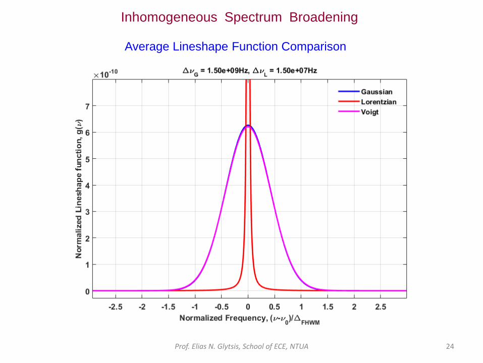
Inhomogeneous Spectrum Broadening
Average Lineshape Function Comparison
ΔνG
ΔνL
ΔνV
Prof. Elias N. Glytsis, School of ECE, NTUA 24
Inhomogeneous Spectrum Broadening
Average Lineshape Function Comparison
Prof. Elias N. Glytsis, School of ECE, NTUA 25
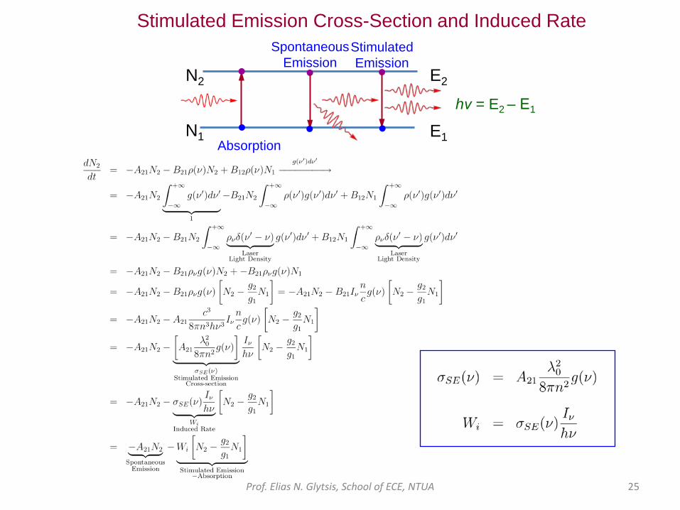
Stimulated Emission Cross-Section and Induced Rate
E1
E2
N1
N2
hν = E2 ‒ E1
Absorption
Spontaneous Emission
Stimulated Emission
Prof. Elias N. Glytsis, School of ECE, NTUA 26
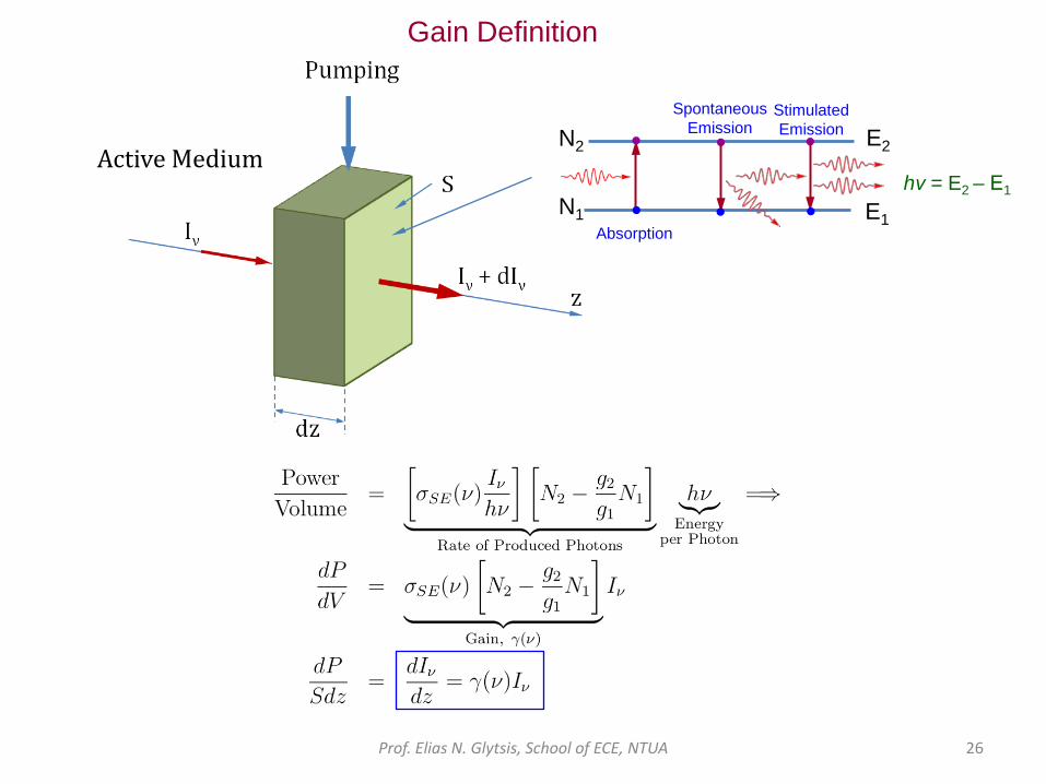
Gain Definition
E1
E2
N1
N2
hν = E2 ‒ E1
Absorption
Spontaneous Emission
Stimulated Emission
Active Medium

Prof. Elias N. Glytsis, School of ECE, NTUA 27
hν = E2 ‒ E1
E2, τ2
E0
N1
N2
N0
R1
R2
E1, τ1 1/τ20
1/τ1
abs
sp.em. st.em.
Gain Saturation
Rate Equations
Mass Conservation
Prof. Elias N. Glytsis, School of ECE, NTUA 28
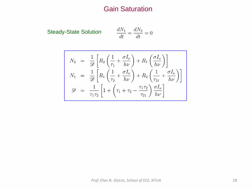
Gain Saturation
Steady-State Solution
Prof. Elias N. Glytsis, School of ECE, NTUA 29
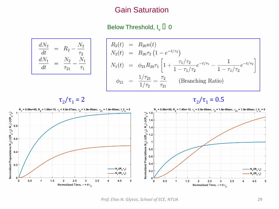
Gain Saturation
Below Threshold, Iν � 0
τ2/τ1 = 2 τ2/τ1 = 0.5
Prof. Elias N. Glytsis, School of ECE, NTUA 30
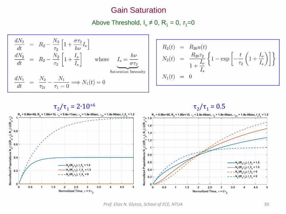
Gain Saturation Above Threshold, Iν ≠ 0, R1 = 0, τ1=0
τ2/τ1 = 2∙10+6 τ2/τ1 = 0.5
Prof. Elias N. Glytsis, School of ECE, NTUA 31
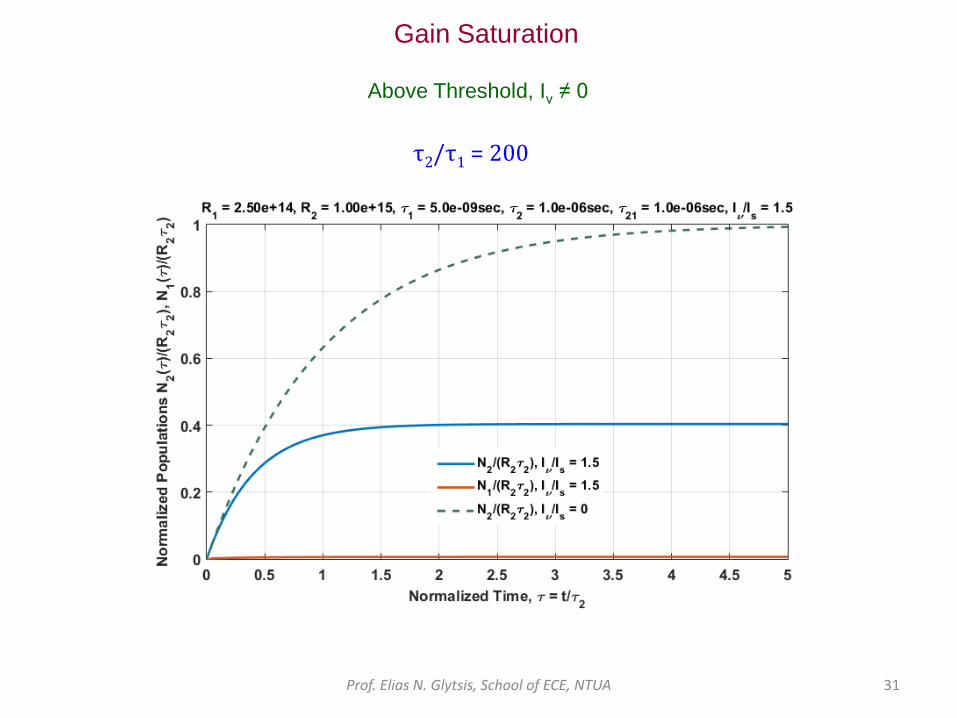
Gain Saturation
Above Threshold, Iν ≠ 0
τ2/τ1 = 200
Prof. Elias N. Glytsis, School of ECE, NTUA 32
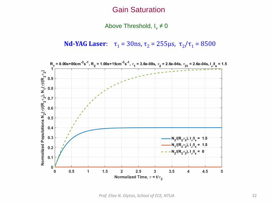
Gain Saturation
Above Threshold, Iν ≠ 0
Nd-YAG Laser: τ1 = 30ns, τ2 = 255μs, τ2/τ1 = 8500

Prof. Elias N. Glytsis, School of ECE, NTUA 33
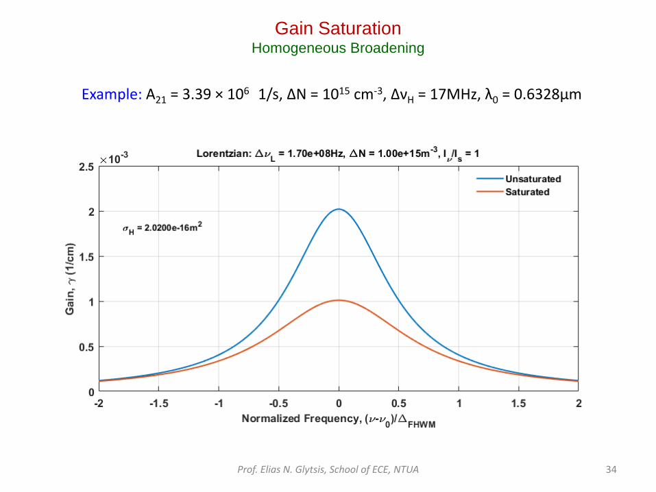
Gain Saturation Homogeneous Broadening
Prof. Elias N. Glytsis, School of ECE, NTUA 34
Gain Saturation Homogeneous Broadening
Example: A21 = 3.39 × 10⁶ 1/s, ΔN = 1015 cm-3, ΔνH = 17MHz, λ0 = 0.6328μm
Prof. Elias N. Glytsis, School of ECE, NTUA 35
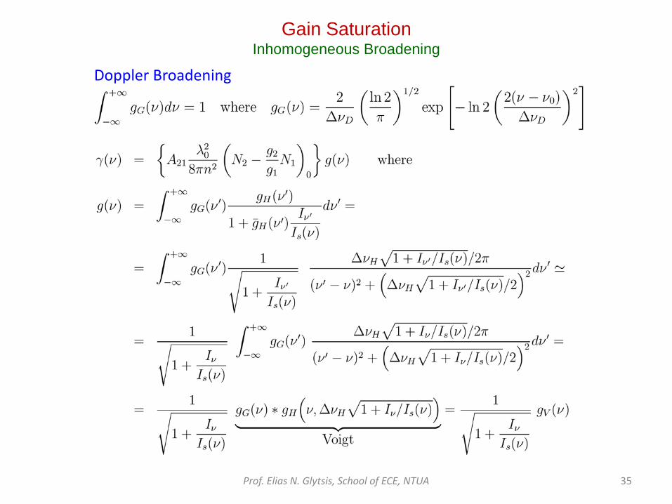
Gain Saturation Inhomogeneous Broadening
Doppler Broadening
Prof. Elias N. Glytsis, School of ECE, NTUA 36
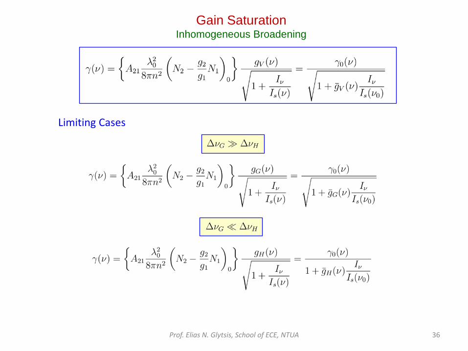
Gain Saturation Inhomogeneous Broadening
Limiting Cases
Prof. Elias N. Glytsis, School of ECE, NTUA 37
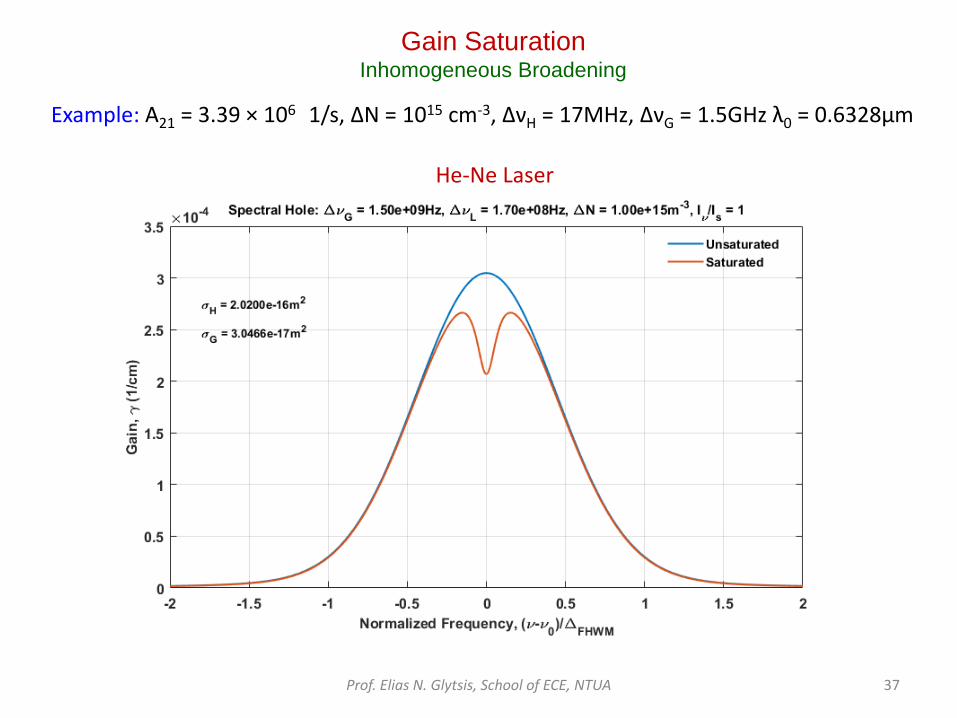
Gain Saturation Inhomogeneous Broadening
Example: A21 = 3.39 × 10⁶ 1/s, ΔN = 1015 cm-3, ΔνH = 17MHz, ΔνG = 1.5GHz λ0 = 0.6328μm
He-Ne Laser
Prof. Elias N. Glytsis, School of ECE, NTUA 38
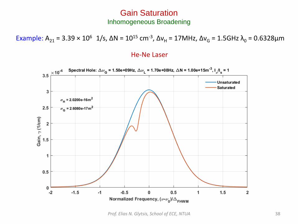
Gain Saturation Inhomogeneous Broadening
Example: A21 = 3.39 × 10⁶ 1/s, ΔN = 1015 cm-3, ΔνH = 17MHz, ΔνG = 1.5GHz λ0 = 0.6328μm
He-Ne Laser

Prof. Elias N. Glytsis, School of ECE, NTUA 39
Gain Saturation Inhomogeneous Broadening
Example: A21 = 3.39 × 10⁶ 1/s, ΔN = 1015 cm-3, ΔνH = 17MHz, ΔνG = 1.5GHz λ0 = 0.6328μm
He-Ne Laser

Prof. Elias N. Glytsis, School of ECE, NTUA 40
Gain Saturation Homogeneous & and Inhomogeneous Broadening
From J. T. Verdeyen, “Laser Electronics” 3rd Ed. Prentice Hall, 1995
Homogeneous Broadening
Inhomogeneous Broadening

Prof. Elias N. Glytsis, School of ECE, NTUA 41
Electron Motion Equation
Classical Electron Oscillator Model
+
- - -
-
-
- -
-
-
+
E = 0 E � 0 z
E s(t) p
Simple Atom Model
External Electric Field

Prof. Elias N. Glytsis, School of ECE, NTUA 42
Classical Electron Oscillator Model Fourier Transform Pairs Electron Motion Equation
Electric Dipole Moment
Macroscopic Polarization

Prof. Elias N. Glytsis, School of ECE, NTUA 43
Classical Electron Oscillator Model
Macroscopic Polarization
He-Ne laser Example (inversion of N = 1010 cm-3 )

Prof. Elias N. Glytsis, School of ECE, NTUA 44
Stimulated Emission

Prof. Elias N. Glytsis, School of ECE, NTUA 45
(a) Parallel plane cavity: Highest mode volume and highest diffraction loss. Difficult to align. (b) The spherical cavity : Represents the functional "opposite" of the plane parallel cavity (a). It is easiest to align, has the lowest diffraction loss, and has the smallest mode volume. CW dye lasers are equipped with this type of cavity because a focused beam is necessary to cause efficient stimulated emission of these lasers. The spherical cavity is not commonly used with any other type of laser. (c) The long radius cavity: Improves on the mode volume, but does so at the expense of a more difficult alignment and a slightly greater diffraction loss than that of the confocal cavity. This type of cavity is suitable for any CW laser application, but few commercial units incorporate the long radius cavity. (d) The confocal cavity: A compromise between the plane parallel and the spherical cavities. The confocal cavity combines the ease of alignment and low diffraction loss of the spherical cavity with the increased mode volume of the plane parallel. Confocal cavities can be utilized with almost any CW laser, but are not in common use. (e) The hemispherical cavity : Actually is one half of the spherical cavity, and the characteristics of the two are similar. The advantage of this type of cavity over the spherical cavity is the cost of the mirrors. The hemispherical cavity is used with most low power He-Ne lasers because of low diffraction loss, ease of alignment, and reduced cost. (f) The long-radius-hemispherical cavity : Combines the cost advantage of the hemispherical cavity with the improved mode volume of the long-radius cavity. Most CW lasers (except low-power He-Ne lasers) employ this type of cavity. In most cases, r1 > 2L. (g) The concave-convex cavity : Normally is used only with high power CW CO2 lasers. In practice, the diameter of the convex mirror is smaller than that of the beam. The output beam is formed by the part of the beam that passes around the mirror and, consequently, has a "doughnut" configuration. The beam must pass around the mirror because mirrors that will transmit the intense beams of these high-power lasers cannot be constructed.
Common Resonators Types
http://www.repairfaq.org/sam/laserioi.htm#ioiresc
Prof. Elias N. Glytsis, School of ECE, NTUA 46
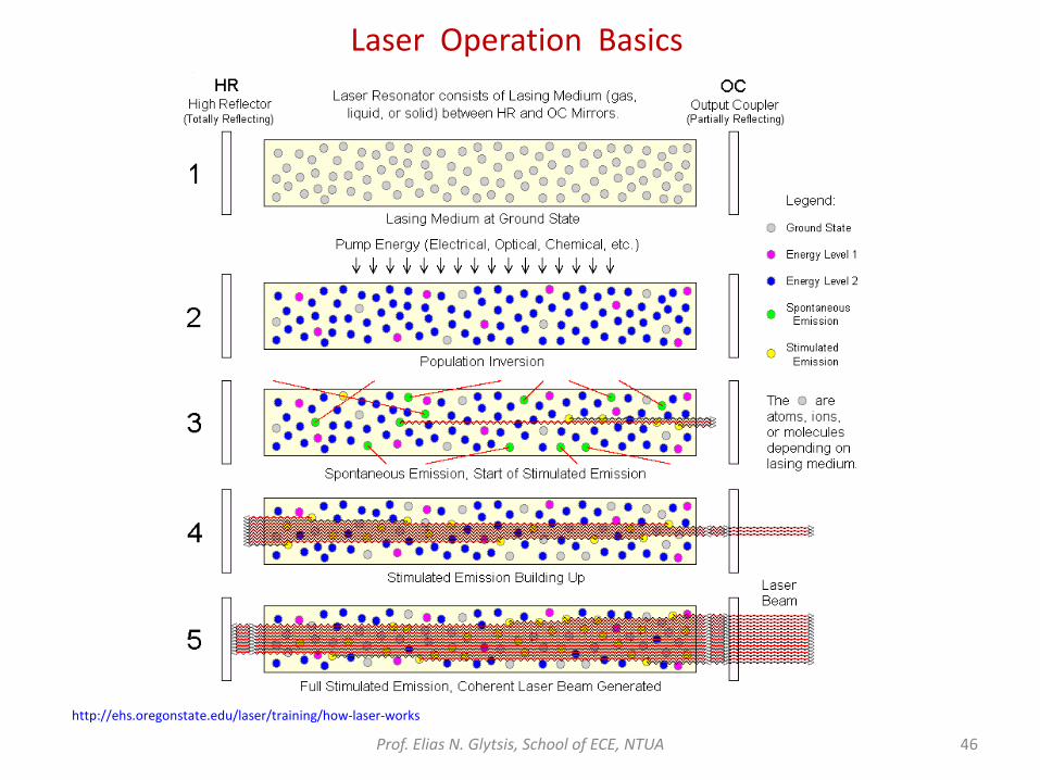
Laser Operation Basics
http://ehs.oregonstate.edu/laser/training/how-laser-works

Prof. Elias N. Glytsis, School of ECE, NTUA 47
Fabry-Perot Laser
E1
E2
N1
N2
hν = E2 ‒ E1
Absorption
Spontaneous Emission
Stimulated Emission
ℓ
Pump

Prof. Elias N. Glytsis, School of ECE, NTUA 48
Fabry-Perot Laser
Resonance Conditions
Threshold Gain

Prof. Elias N. Glytsis, School of ECE, NTUA 49
Fabry-Perot Laser Frequency Pulling
2kℓ [ 1 + χ’/2n2 ]
2πm
2πm
2πm Frequency pulling
Frequency pulling
ν ν0
χ’ 2kℓ
νm νm
(νm-ν0) (Δν1/2/Δν)
-(νm-ν0) (Δν1/2/Δν)

Prof. Elias N. Glytsis, School of ECE, NTUA 50
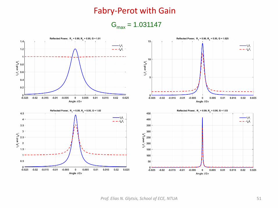
Fabry-Perot with Gain
https://en.wikipedia.org/wiki/File:Etalon-2.svg
Ii
It
Ir
G = 1 (no gain)
Prof. Elias N. Glytsis, School of ECE, NTUA 51
Fabry-Perot with Gain Gmax = 1.031147
Prof. Elias N. Glytsis, School of ECE, NTUA 52
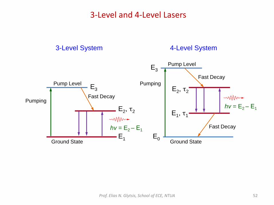
3-Level and 4-Level Lasers
E2, τ2 E1, τ1
E2, τ2
E1
E3
E3
E0
hν = E2 ‒ E1
hν = E2 ‒ E1
Pumping
Pumping
Fast Decay
Fast Decay
Fast Decay
Ground State Ground State
Pump Level
Pump Level
3-Level System 4-Level System

Prof. Elias N. Glytsis, School of ECE, NTUA 53
hν = E2 ‒ E1
E2, τ2
E0
N1
N2
N0
R1
R2
E1, τ1
1/τ1
abs
sp.em. st.em.
Absorption zone
Laser Power Considerations

Prof. Elias N. Glytsis, School of ECE, NTUA 54
Laser Power Considerations
Below Threshold
Above Threshold
Steady-State

Prof. Elias N. Glytsis, School of ECE, NTUA 55
Laser Power Considerations
Power due to Stimulated Emission
Prof. Elias N. Glytsis, School of ECE, NTUA 56
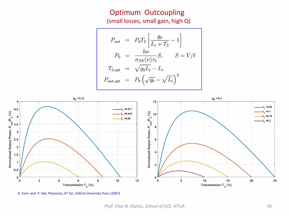
Optimum Outcoupling (small losses, small gain, high Q)
A. Yariv and P. Yeh, Photonics, 6th Ed., Oxford University Press (2007)
Prof. Elias N. Glytsis, School of ECE, NTUA 57
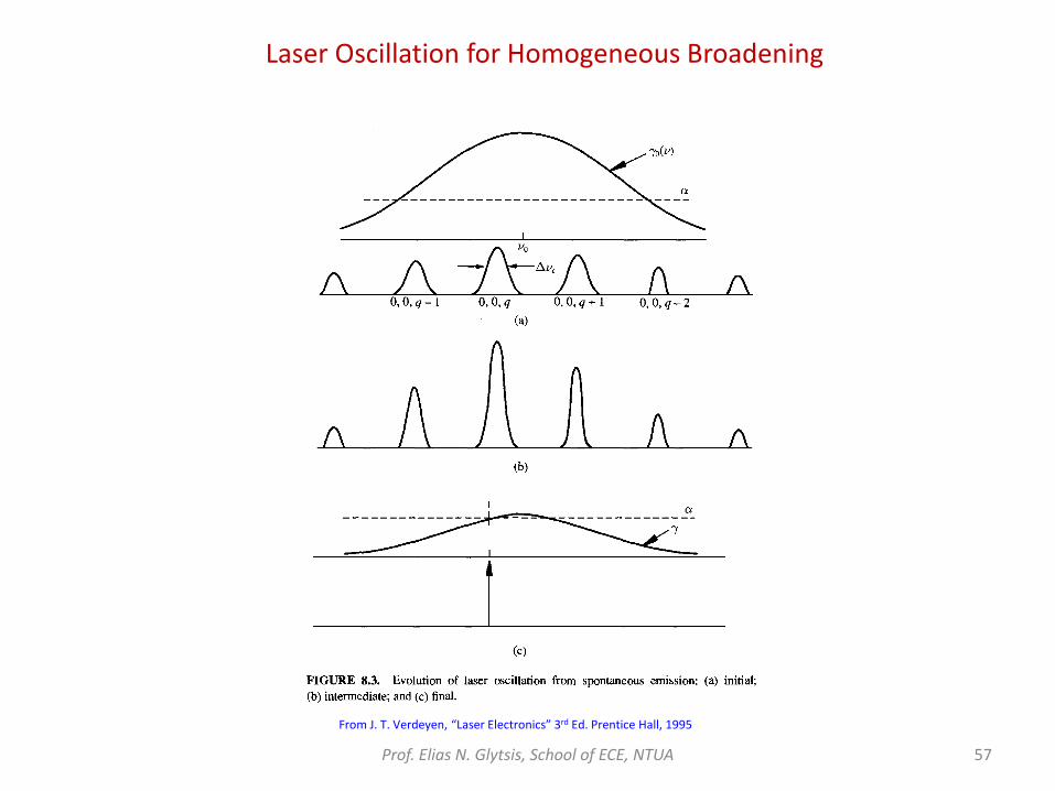
Laser Oscillation for Homogeneous Broadening
From J. T. Verdeyen, “Laser Electronics” 3rd Ed. Prentice Hall, 1995

Prof. Elias N. Glytsis, School of ECE, NTUA 58
Laser Oscillation for Inhomogeneous Broadening

Prof. Elias N. Glytsis, School of ECE, NTUA 59
Laser Oscillation for Inhomogeneous Broadening
From J. T. Verdeyen, “Laser Electronics” 3rd Ed. Prentice Hall, 1995

Prof. Elias N. Glytsis, School of ECE, NTUA 60
Below Threshold
Above Threshold
Coldren and Corzine, Diode Lasers & Photonic Integrated Circuits, J. Wiley (1995)
Prof. Elias N. Glytsis, School of ECE, NTUA 61
From B.E.A. Saleh & M. C. Teich, “Fundamentals of Photonics” 2nd Ed. J. Wiley & Sons,2007.
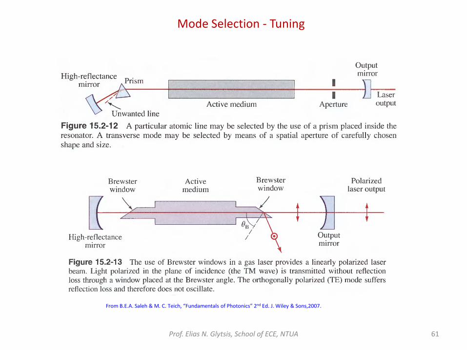
Mode Selection - Tuning
Prof. Elias N. Glytsis, School of ECE, NTUA 62
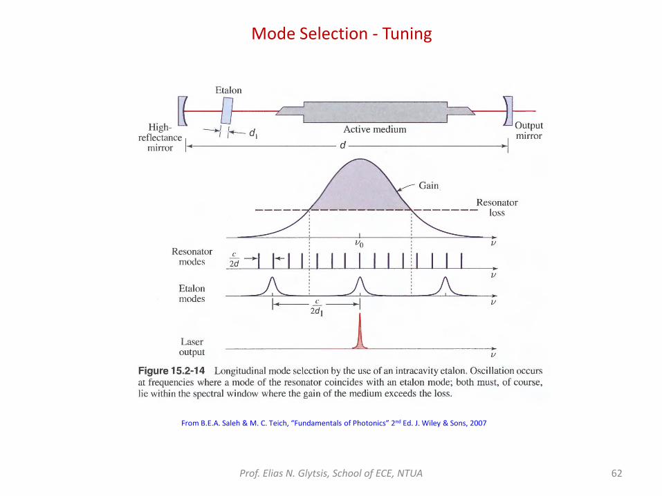
Mode Selection - Tuning
From B.E.A. Saleh & M. C. Teich, “Fundamentals of Photonics” 2nd Ed. J. Wiley & Sons, 2007

Prof. Elias N. Glytsis, School of ECE, NTUA 63
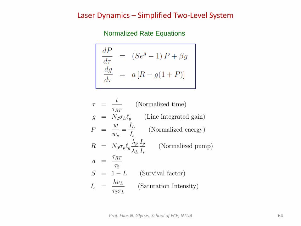
Laser Dynamics – Simplified Two-Level System
E2, τ2
Pump
Lasing
E1, τ1
Ground State
N2
IL
Very fast
R1 R2
R3 R4
Pump
Laser Medium
Output IL
ℓg
Prof. Elias N. Glytsis, School of ECE, NTUA 64
Laser Dynamics – Simplified Two-Level System
Normalized Rate Equations
Prof. Elias N. Glytsis, School of ECE, NTUA 65
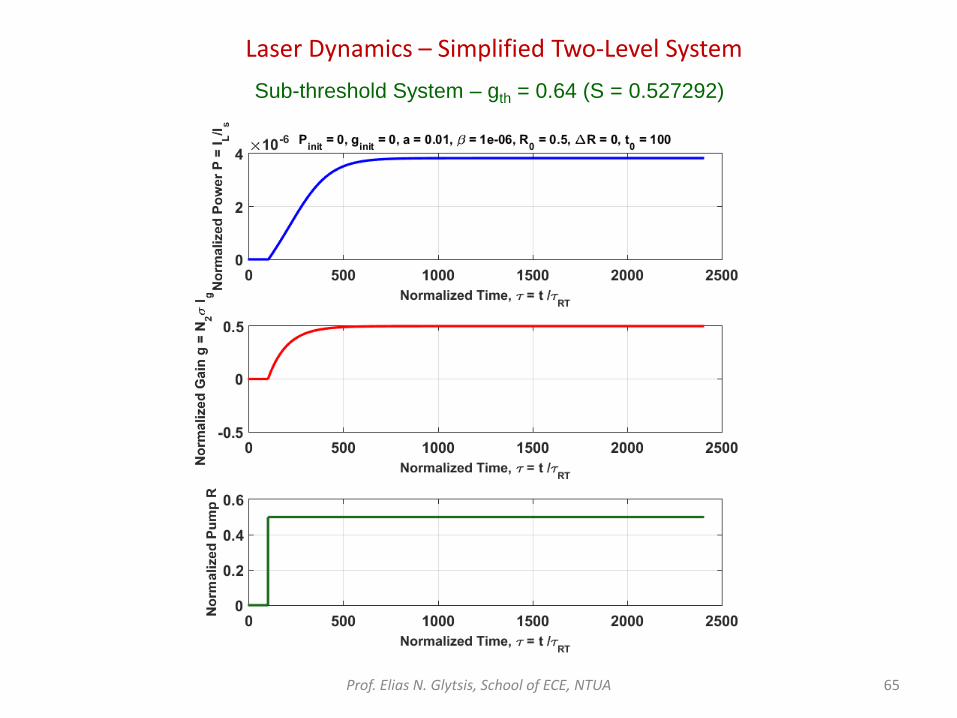
Laser Dynamics – Simplified Two-Level System Sub-threshold System – gth = 0.64 (S = 0.527292)
Prof. Elias N. Glytsis, School of ECE, NTUA 66
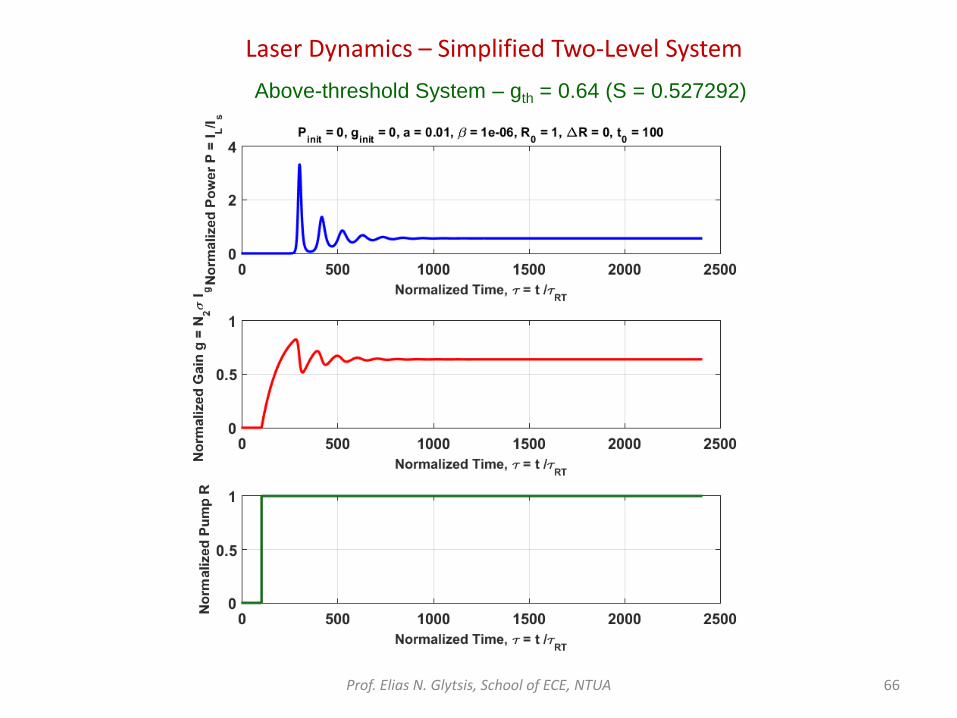
Laser Dynamics – Simplified Two-Level System Above-threshold System – gth = 0.64 (S = 0.527292)
Prof. Elias N. Glytsis, School of ECE, NTUA 67
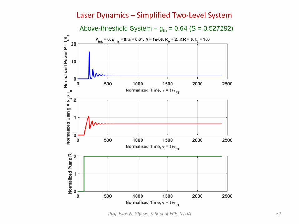
Laser Dynamics – Simplified Two-Level System Above-threshold System – gth = 0.64 (S = 0.527292)

Prof. Elias N. Glytsis, School of ECE, NTUA 68
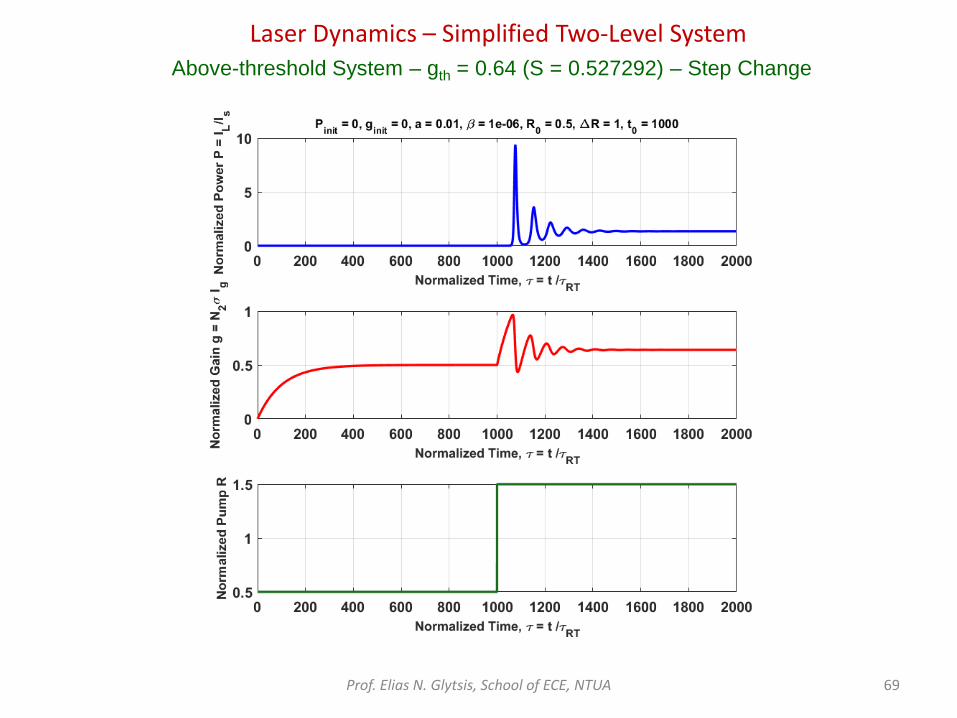
Laser Dynamics – Simplified Two-Level System Above-threshold System – gth = 0.64 (S = 0.527292) – Step Change
Prof. Elias N. Glytsis, School of ECE, NTUA 69
Laser Dynamics – Simplified Two-Level System Above-threshold System – gth = 0.64 (S = 0.527292) – Step Change
Prof. Elias N. Glytsis, School of ECE, NTUA 70
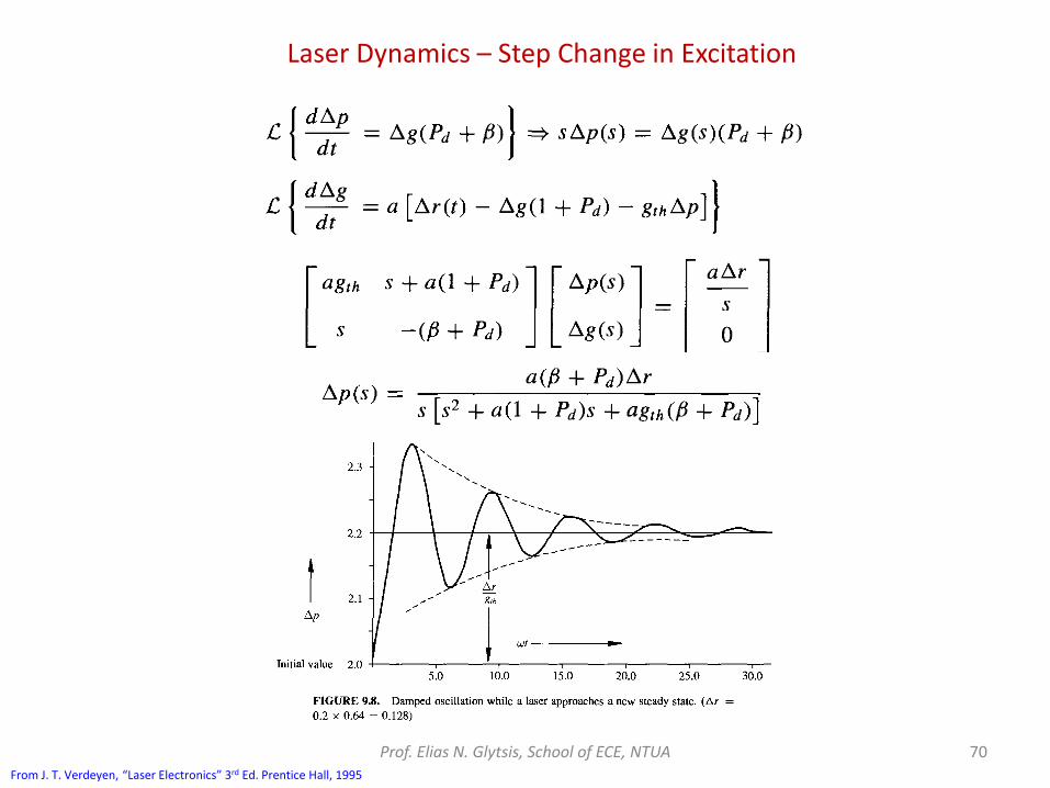
Laser Dynamics – Step Change in Excitation
From J. T. Verdeyen, “Laser Electronics” 3rd Ed. Prentice Hall, 1995

Prof. Elias N. Glytsis, School of ECE, NTUA 71 From J. T. Verdeyen, “Laser Electronics” 3rd Ed. Prentice Hall, 1995
Sinusoidal Response – gth = 0.64 (S = 0.527292)
Laser Dynamics – Simplified Two-Level System
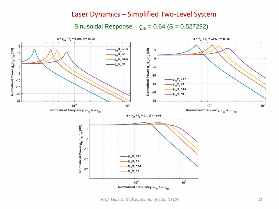
Prof. Elias N. Glytsis, School of ECE, NTUA 72
Laser Dynamics – Simplified Two-Level System Sinusoidal Response – gth = 0.64 (S = 0.527292)

Prof. Elias N. Glytsis, School of ECE, NTUA 73
Mode Locking – Time Domain Consideration
From A. Siegman, “Lasers”, Univ. Science Books, 1986

Prof. Elias N. Glytsis, School of ECE, NTUA 74
Mode Locking – Time Domain Consideration
From A.E. Siegman, “Lasers”, Univ. Science Books, 1986

Prof. Elias N. Glytsis, School of ECE, NTUA 75
Mode Locking – Frequency Domain Consideration
From J. T. Verdeyen, “Laser Electronics”, 3rd Ed., Prentice Hall, 1995

Prof. Elias N. Glytsis, School of ECE, NTUA 76
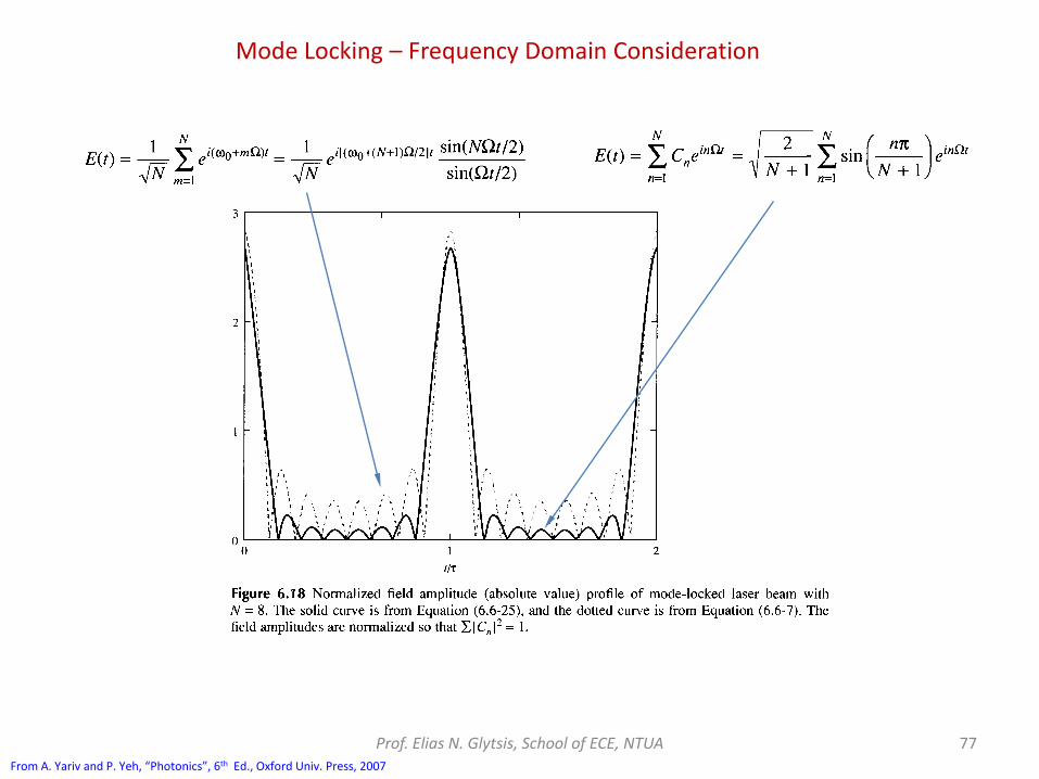
Mode Locking – Frequency Domain Consideration
From J. T. Verdeyen, “Laser Electronics”, 3rd Ed., Prentice Hall, 1995
Prof. Elias N. Glytsis, School of ECE, NTUA 77
Mode Locking – Frequency Domain Consideration
From A. Yariv and P. Yeh, “Photonics”, 6th Ed., Oxford Univ. Press, 2007

Prof. Elias N. Glytsis, School of ECE, NTUA 78
Mode Locking – Frequency Domain Consideration
From A.E. Siegman, “Lasers”, Univ. Science Books, 1986

Prof. Elias N. Glytsis, School of ECE, NTUA 79
Mode Locking – Frequency Domain Consideration
L = 1m, n = 1, λ0 = 1μm, Δν = 1.50e+09Hz

Prof. Elias N. Glytsis, School of ECE, NTUA 80
Mode Locking – Frequency Domain Consideration
L = 2m, n = 1, λ0 = 1μm, Δν = 1.50e+09Hz
Prof. Elias N. Glytsis, School of ECE, NTUA 81
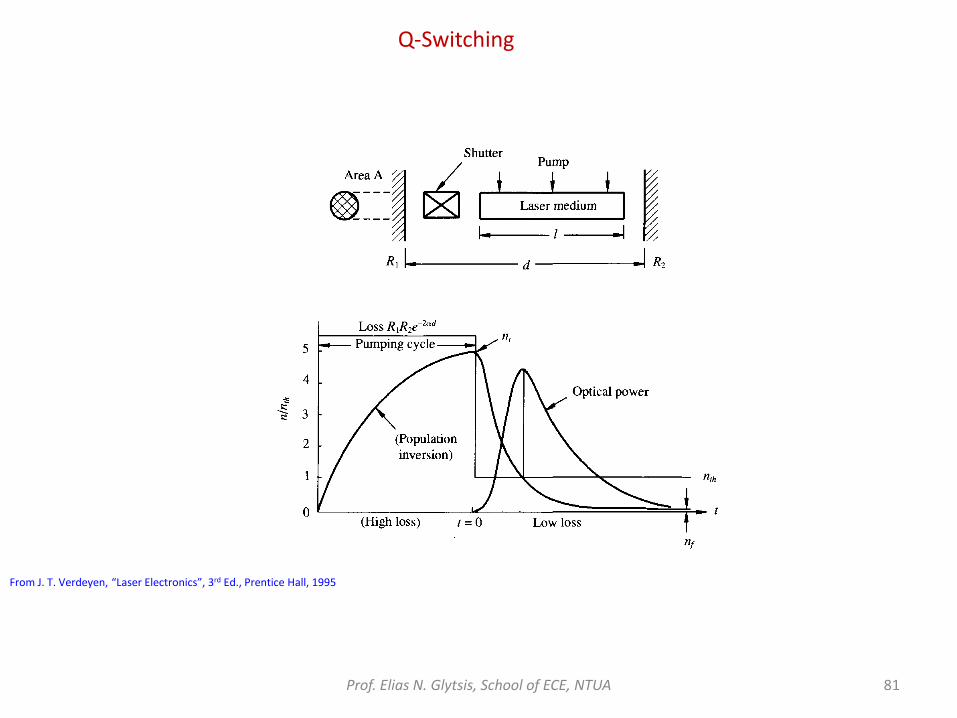
Q-Switching
From J. T. Verdeyen, “Laser Electronics”, 3rd Ed., Prentice Hall, 1995
Prof. Elias N. Glytsis, School of ECE, NTUA 82
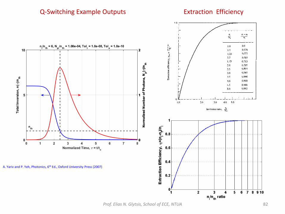
A. Yariv and P. Yeh, Photonics, 6th Ed., Oxford University Press (2007)
Q-Switching Example Outputs Extraction Efficiency
Prof. Elias N. Glytsis, School of ECE, NTUA 83
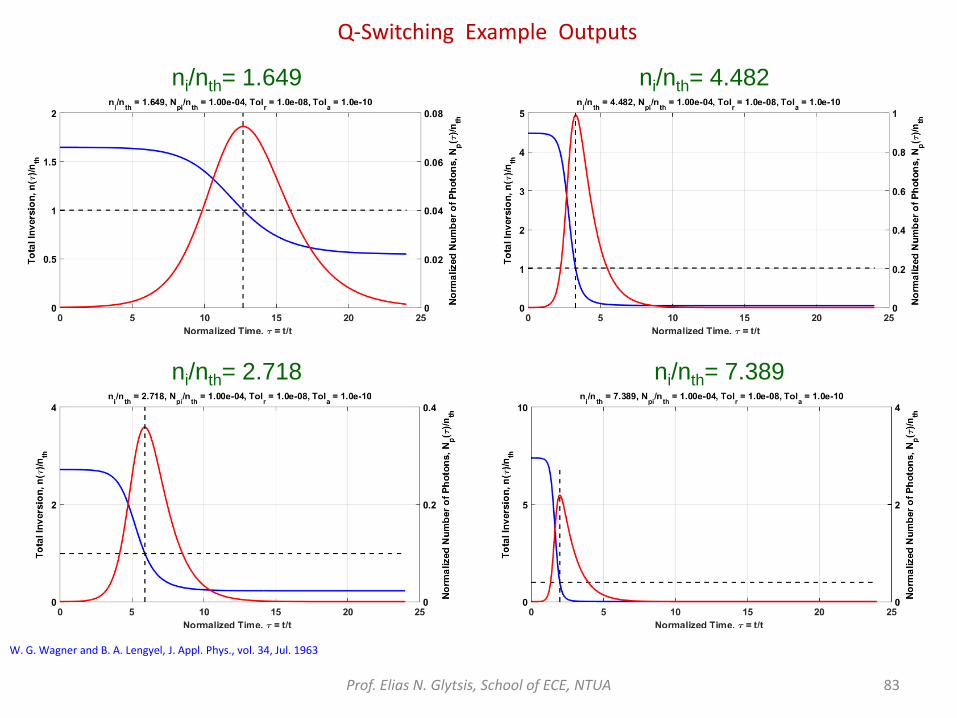
Q-Switching Example Outputs
ni/nth= 1.649 ni/nth= 4.482
ni/nth= 2.718 ni/nth= 7.389
W. G. Wagner and B. A. Lengyel, J. Appl. Phys., vol. 34, Jul. 1963


