
Conjunction Assessment Risk Analysis
M.D. Hejduk
13 APR 2016
Late-Notice
HIE
Investigation
https://ntrs.nasa.gov/search.jsp?R=20160005111 2018-05-29T21:46:58+00:00Z
M.D. Hejduk | Late-Notice HIEs | 13 APR 2016 | 2
Purpose
• Provide a response to MOWG action item 1410-01:
– Analyze close approaches which have required mission team action on
short notice. Determine why the approaches were identified later in the
process than most other events.
• Method:
– Performed an analysis to determine whether there is any correlation
between late notice event identification and space weather, sparse
tracking, or high drag objects,which would allow preventive action to be
taken
– Examined specific late notice events identified by missions as
problematic to try to identify root cause and attempt to relate them to the
correlation analysis

M.D. Hejduk | Late-Notice HIEs | 13 APR 2016 | 3
Agenda
• Frequency/correlation of large state changes
– Individual states of primary and secondary objects
• Overall frequency of ε/σ and comparison to theoretical frequencies
• Pc vs primary and secondary ε/σ size
• Secondary ε/σ vs tracking level and vs energy dissipation rate (EDR)
– Combined states: component miss distances vs combined covariance
• Overall frequency of ε/σ and comparison to theoretical frequencies
• Pc vs ε/σ size; ε/σ vs tracking levels, EDR
• ε/σ vs F10, average Ap, and peak Ap
– Preliminary conclusions
• Case studies of four late-notice events
• Overall conclusions and way forward

M.D. Hejduk | Late-Notice HIEs | 13 APR 2016 | 4
Dataset to Analyze
• All reported conjunctions for ca. 700 km defended missions
– Landsat-7, Terra, EO-1, Aqua, Aura, CloudSat, CALIPSO, GCOM-W1,
Landsat-8, OCO-2, SMAP
• Data interval from 1 MAY 2015 to 1 FEB 2016
– New Dynamic Consider Parameter (DCP) functionality installed on ASW on
May 1, 2016, so covariance realism purported to be much improved
• All CDM updates examined within every event (not just initial
identification)
M.D. Hejduk | Late-Notice HIEs | 13 APR 2016 | 5
Broad Investigation of Large State Changes
• Determine actual frequency of large state changes, in both
individual and combined states
– Compare to theoretically expected frequencies
• Determine whether broadly correlated with potential/expected
causes
– Low tracking
– Harder-to-maintain orbits (larger energy dissipation rate)
– General levels of solar activity (EUV and Joule atmospheric heating)
M.D. Hejduk | Late-Notice HIEs | 13 APR 2016 | 6
Large State Changes:
Parameterization (1 of 3)
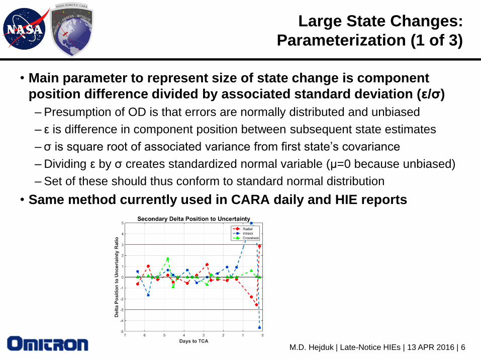
• Main parameter to represent size of state change is component
position difference divided by associated standard deviation (ε/σ)
– Presumption of OD is that errors are normally distributed and unbiased
– ε is difference in component position between subsequent state estimates
– σ is square root of associated variance from first state’s covariance
– Dividing ε by σ creates standardized normal variable (μ=0 because unbiased)
– Set of these should thus conform to standard normal distribution
• Same method currently used in CARA daily and HIE reports
M.D. Hejduk | Late-Notice HIEs | 13 APR 2016 | 7
Large State Changes:
Parameterization (2 of 3)
• However . . . This is only true for the “diagonalized” situation, in
which covariance axes and coordinate frame axes align
– Results meaningful only if ellipse closely aligns with coordinate axes
– Once ellipse rotated, then component errors are correlated
• Individual component error distributions no longer independent random variables
• How often are covariance error ellipsoids naturally diagonalized?
– Not terrible assumption for individual satellites (primary, secondary)
– More tenuous for combined situation (miss distance vs combined covariance)
• Bottom line: ε/σ statistics at the component level must be used with
care
– When plotted against only positive axis, presume ε/σ to be abs(ε/σ)

M.D. Hejduk | Late-Notice HIEs | 13 APR 2016 | 8
Large State Changes:
Parameterization (3 of 3)
• Comparison alternative: Mahalanobis distance
– If individual component errors normally distributed, then sum of squares of
individual ratios (ε2/σ2) will constitute a 3-DoF χ2 distribution
– Formulary εC-1εT properly considers all correlations and makes the calculation
independent of coordinate system
– Approach less frequently encountered, so less intuition built up around result
– But will be supplied and examined along with Gaussian variables
– Can also examine 2-DoF situation for only radial and in-track
• More information on this later
M.D. Hejduk | Late-Notice HIEs | 13 APR 2016 | 9
Issues in Comparison to Theory
• Commonly-known “percentages” for univariate Gaussian
distribution consider two-tailed results
– 95.4% for 2-σ distribution considers results from 2.3% to 97.7%
– 99.7% for 3-σ distribution considers results from 0.15% to 99.85%
• Potential double-counting of large state changes
– Subsequent updates analyzed for large state change behavior
– In a chain of updates, return to normalcy will appear as a second large change
– Demarcation between one and two events not so easy to define
(S = small state change; L = large state change
• S S L L S S – one or two events?
• S S S L S S L S S – one or two events?
• S S S S S S L – one or two events (would it have been counted as two if one more
update had been available?
– For data-mining simplicity, all large changes counted, with the caveat that
reported number might be twice as large as “actual” number

N. Sabey | ERB | 18 Jun 2013 | 10
STATE-CHANGE FREQUENCY AND
COMPARISON TO THEORY
Primary and Secondary Treated Individually

M.D. Hejduk | Late-Notice HIEs | 13 APR 2016 | 11
Frequency of Large State Changes:
Secondary Objects

M.D. Hejduk | Late-Notice HIEs | 13 APR 2016 | 12
Secondary Large State Changes:
3-σ Comparison to Theory
• Radial frequency a little more than twice theoretical prediction
– 1.3% of updates > 3-σ change
– If all events were double-counted, then would expect 0.6%--have a little more
than double this
• In-track frequency greater than theory
– ~3.3%; greater than theory by perhaps factor of five
– Component most heavily affected by expected modeling errors
• Cross-track component performs surprisingly badly
– ~7.0% of updates; substantially greater than theory
– Can be largely attributed to very small sigma values
• Will be addressed in more depth later
• How often do these matter?
– If occur nearly always for low-Pc events, then perhaps not much

M.D. Hejduk | Late-Notice HIEs | 13 APR 2016 | 13
Secondary Large State Changes:
Frequency in Situations that Matter
• Change > 3σ and max Pc for event > 1E-05
– Radial = 0.3%, in-track = 0.4%, cross-track = 0.9%
• Change > 3σ, max Pc for event > 1E-05, and Pc change after “large”
change > 1 order of magnitude
– Radial = 0.07%, in-track = 0.13%, cross-track = 0.15%
• Change > 3σ, max Pc for event > 1E-05, and Pc change after “large”
change > 2 orders of magnitude
– Radial = 0.05%, in-track = 0.12%, cross-track = 0.09%
• Percentages perhaps as much as double “real” values
• Sampling is not large enough to allow robust comparison to theory
at the 3σ level
Overall, prevalence is greater than theory would predict.
However, presence in events of significance notably reduced

M.D. Hejduk | Late-Notice HIEs | 13 APR 2016 | 14
Frequency of Large State Changes:
Primary Objects
M.D. Hejduk | Late-Notice HIEs | 13 APR 2016 | 15
Summary of Frequencies:
Primary and Secondary Objects
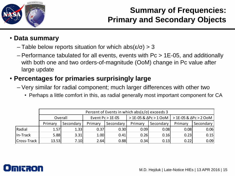
• Data summary
– Table below reports situation for which abs(ε/σ) > 3
– Performance tabulated for all events, events with Pc > 1E-05, and additionally
with both one and two orders-of-magnitude (OoM) change in Pc value after
large update
• Percentages for primaries surprisingly large
– Very similar for radial component; much larger differences with other two
• Perhaps a little comfort in this, as radial generally most important component for CA
Primary Secondary Primary Secondary Primary Secondary Primary Secondary
Radial 1.57 1.33 0.37 0.30 0.09 0.08 0.08 0.06
In-Track 5.88 3.31 1.00 0.41 0.26 0.16 0.23 0.15
Cross-Track 13.53 7.10 2.64 0.88 0.34 0.13 0.22 0.09
Overall Event Pc > 1E-05 > 1E-05 & ΔPc > 1 OoM > 1E-05 & ΔPc > 2 OoM
Percent of Events in which abs(ε/σ) exceeds 3
M.D. Hejduk | Late-Notice HIEs | 13 APR 2016 | 16
Comparison of ε/σ to Theory:
Primary and Secondary Objects

M.D. Hejduk | Late-Notice HIEs | 13 APR 2016 | 17
Comparison of ε/σ to Theory:
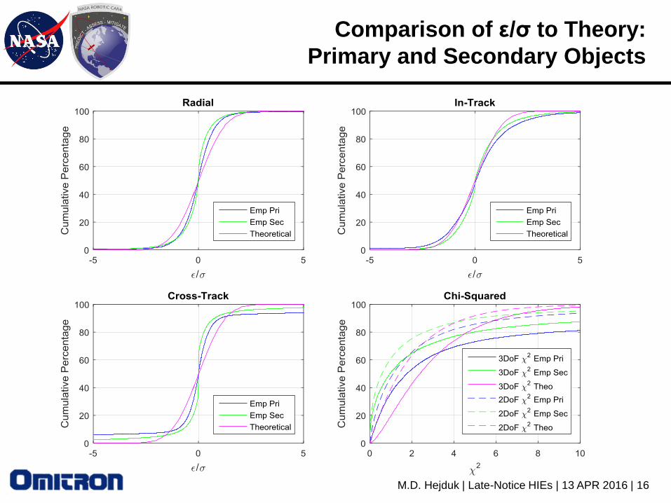
Interpretation
• Radial behaves reasonably well—better than theory until more
extreme part of tails reached
– Cannot see tail behavior very well in provided plots
• In-track has non-theoretical distribution beyond about ε/σ > 1
– As remarked previously, worse for secondaries than for primaries
• Cross-track highly leptokurtic—peaked with very long tails
– Does not match a Gaussian distribution at all
• In using chi-squared distribution, 2-DoF framework gives more
sanguine situation
– Eliminates effect of large cross-track differences
– Nonetheless, non-theory outliers dominate performance in the tails
• None of these results sets match the theory particularly well
• Immediate conclusion difficult
– OD residuals suspected to be leptokurtic
– Present trend could be extension of this
M.D. Hejduk | Late-Notice HIEs | 13 APR 2016 | 18
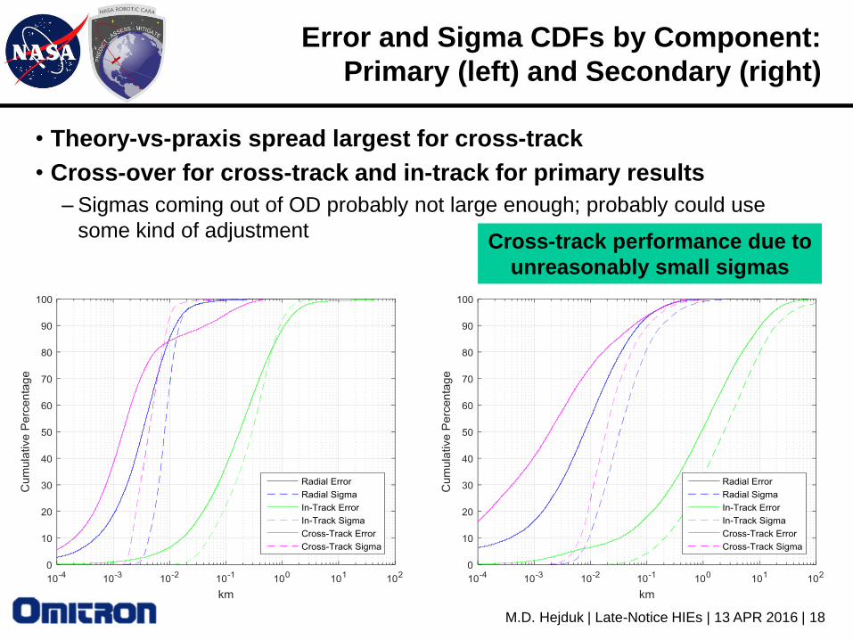
Error and Sigma CDFs by Component:
Primary (left) and Secondary (right)
• Theory-vs-praxis spread largest for cross-track
• Cross-over for cross-track and in-track for primary results
– Sigmas coming out of OD probably not large enough; probably could use
some kind of adjustmentCross-track performance due to
unreasonably small sigmas

M.D. Hejduk | Late-Notice HIEs | 13 APR 2016 | 19
CORRELATION INVESTIGATIONS
Primary and Secondary Treated Individually

M.D. Hejduk | Late-Notice HIEs | 13 APR 2016 | 20
Correlation Indices
• Correlation tests indicate the degree to which two variables are
correlated
– Range of values is -1 to 1
– 1 indicates perfect correlation;
-1 indicates perfect inverse correlation;
0 indicates no correlation
• Three correlation indices in general use
– Pearson correlation coefficient: tests for linear correlation
• What most people learn in statistics class
• Evaluates how well two datasets exhibit a linear relationship
– Kendall’s tau and Spearman’s rho: test for rank correlation
• Much less frequently taught but more powerful
• Evaluate how well two datasets move in the same (or opposite) directions
• All three used in present analysis to examine data correlations

M.D. Hejduk | Late-Notice HIEs | 13 APR 2016 | 21
Pearson Correlation Coefficient
• Evaluates the degree of a linear relationship between two variables
• Usually evaluated by the formula (s is sample standard deviation),
with range of interesting and often not helpful outcomes
• Some interpretive guidance via relationship to r2 value from linear
regression: square of Pearson = regression r2
– Pearson value of 0.5 would equate to r2 of 0.25—not very impressive
• Really would like something that reveals even non-linear correlation
y
in
i x
i
s
yy
s
xx
nr
11
1
M.D. Hejduk | Late-Notice HIEs | 13 APR 2016 | 22
Kendall’s Tau
• Rank correlation test
– With two vectors of data X and Y, compares (Xi,Yi) to every other (Xj,Yj)
– Pair is concordant if, when Xi>Xj, Yi>Yj; discordant if the opposite
– Parameter is (# concordant pairs - # discordant pairs) / (total pairs)
• So same range of values (-1 to 1) with same meaning
• Much more robust test
– Will find both linear and nonlinear correlation
– Computationally expensive [~O(n2)], but computers are doing the work
• Tied situations create problems
– In present analysis, arises when comparing continuous to discrete distribution
• e.g., ε/σ to tracking levels (because tracking levels are counting numbers, so can
have multiple ε/σ values aligned with same tracking level)
– Even more computationally expensive modifications to adjust for ties
– Spot-checked these and saw no difference in computed result

M.D. Hejduk | Late-Notice HIEs | 13 APR 2016 | 23
Spearman’s Rho
• Test of monotonicity, computed by summing squares of differences
in rank
– Mapped into same -1 to 1 range of values, with same interpretation
• Computational formula
• Computationally easier but more vulnerable to outlier data
• Usually larger than Kendall’s tau
• Included here for consistency/contrast
1
6
12
1
2
nn
dn
i
i
Main factor to consult is Kendall’s Tau
M.D. Hejduk | Late-Notice HIEs | 13 APR 2016 | 24
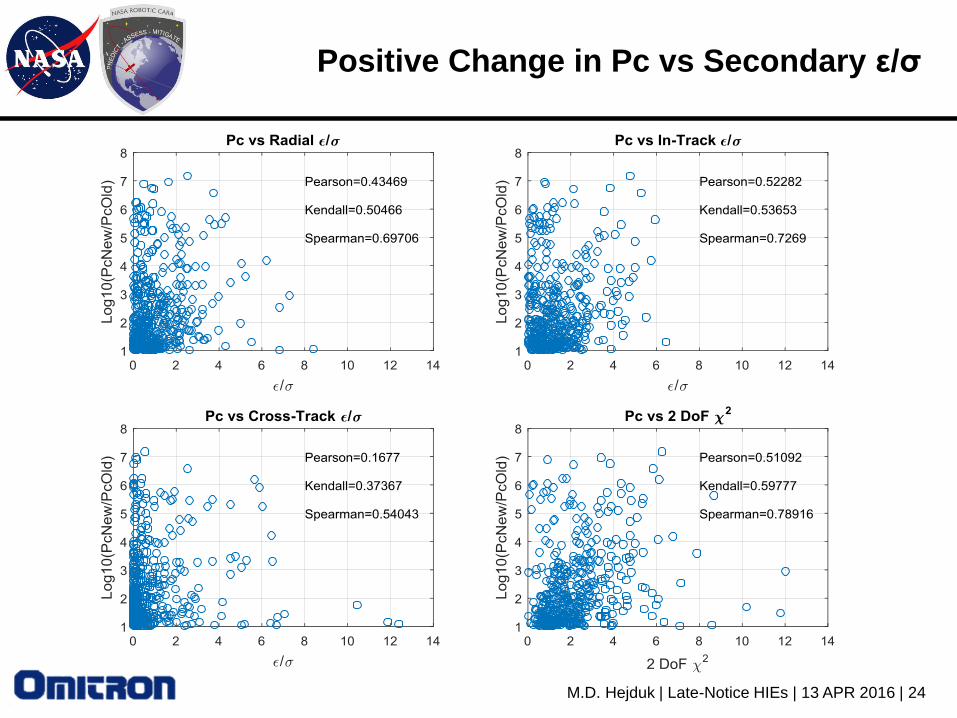
Positive Change in Pc vs Secondary ε/σ
M.D. Hejduk | Late-Notice HIEs | 13 APR 2016 | 25
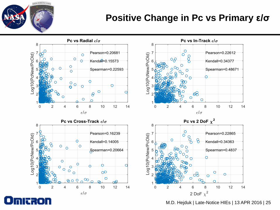
Positive Change in Pc vs Primary ε/σ

M.D. Hejduk | Late-Notice HIEs | 13 APR 2016 | 26
Positive Pc change vs ε/σ:
Summary
• Summary table (Kendall’s Tau):
• Pc correlation with large state changes in primary not very strong
• Pc correlation with large state changes in secondary of some
significance, but still not overwhelming
Radial In-Track Cx-Track Chi-Sq
Primary 0.15 0.34 0.14 0.34
Secondary 0.50 0.54 0.37 0.60
Large state changes in the secondary do correlate
to large changes in Pc, but not all that strongly

M.D. Hejduk | Late-Notice HIEs | 13 APR 2016 | 27
ε/σ vs # of Tracks in Secondary OD:
All Data

M.D. Hejduk | Late-Notice HIEs | 13 APR 2016 | 28
ε/σ vs # of Tracks in Secondary OD:
Radial or In-Track abs(ε/σ) > 3

M.D. Hejduk | Late-Notice HIEs | 13 APR 2016 | 29
ε/σ vs # of Tracks in Secondary OD:
Radial or In-Track abs(ε/σ) > 5
M.D. Hejduk | Late-Notice HIEs | 13 APR 2016 | 30
ε/σ vs # of Tracks in Secondary OD:
Interpretation
• Correlations low, even for high-change events
• More tellingly, should produce inverse correlation but instead see
positive correlation
• Difficult to conclude that unexpectedly large errors are associated
with light tracking
Sparse tracking for secondary
does not correlate with large state errors

M.D. Hejduk | Late-Notice HIEs | 13 APR 2016 | 31
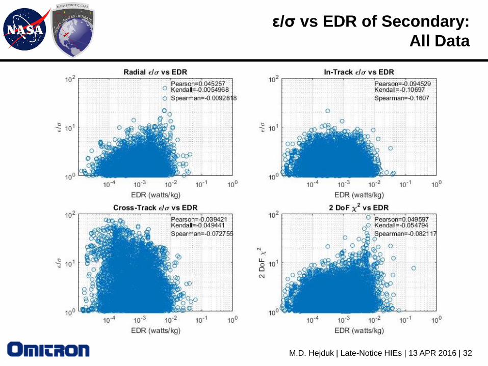
Energy Dissipation Rate
• In 2001 study, Omitron investigated single-value representation of
effect of atmospheric drag
• Proposed concept of the energy dissipation rate (EDR)
– Dot product of inertial drag acceleration vector and inertial velocity vector
– Units of watts per kilogram
– Represents amount of energy being removed from the orbit
– Occasionally amount of energy being added to orbit, such as by solar wind
• EDR can serve as single-value encapsulation of ballistic coefficient
and atmospheric density
VAtEDR D
)(
M.D. Hejduk | Late-Notice HIEs | 13 APR 2016 | 32
ε/σ vs EDR of Secondary:
All Data

M.D. Hejduk | Late-Notice HIEs | 13 APR 2016 | 33
ε/σ vs EDR of Secondary :
Radial or In-Track abs(ε/σ) > 3
M.D. Hejduk | Late-Notice HIEs | 13 APR 2016 | 34
ε/σ vs EDR of Secondary:
Radial or In-Track abs(ε/σ) > 5

M.D. Hejduk | Late-Notice HIEs | 13 APR 2016 | 35
ε/σ vs EDR of Secondary:
Interpretation
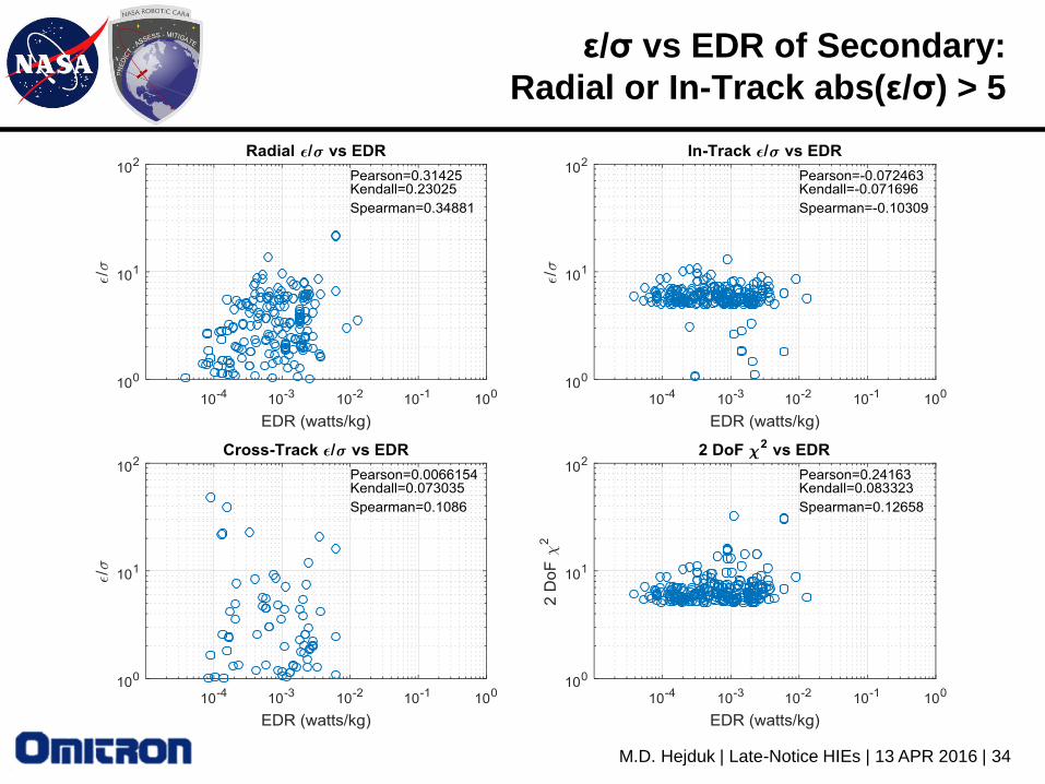
• Correlation rather weak
• Somewhat stronger correlation when dataset limited to the higher
ε/σ values, but even then not significant
Higher EDR values for secondary
do not correlate with larger state errors

M.D. Hejduk | Late-Notice HIEs | 13 APR 2016 | 36
STATE-CHANGE FREQUENCY AND
COMPARISON TO THEORY
Combined Situation

M.D. Hejduk | Late-Notice HIEs | 13 APR 2016 | 37
Frequency of Large State Changes:
Miss vs Combined Sigma
M.D. Hejduk | Late-Notice HIEs | 13 APR 2016 | 38
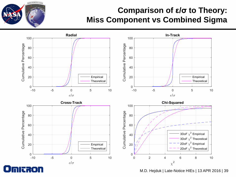
Frequency of Large State Changes:
Tabular Summary
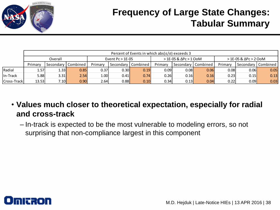
• Values much closer to theoretical expectation, especially for radial
and cross-track
– In-track is expected to be the most vulnerable to modeling errors, so not
surprising that non-compliance largest in this component
Primary Secondary Combined Primary Secondary Combined Primary Secondary Combined Primary Secondary Combined
Radial 1.57 1.33 0.85 0.37 0.30 0.19 0.09 0.08 0.06 0.08 0.06 0.05
In-Track 5.88 3.31 2.54 1.00 0.41 0.74 0.26 0.16 0.16 0.23 0.15 0.13
Cross-Track 13.53 7.10 0.90 2.64 0.88 0.10 0.34 0.13 0.04 0.22 0.09 0.03
> 1E-05 & ΔPc > 2 OoMOverall Event Pc > 1E-05 > 1E-05 & ΔPc > 1 OoM
Percent of Events in which abs(ε/σ) exceeds 3
M.D. Hejduk | Late-Notice HIEs | 13 APR 2016 | 39
Comparison of ε/σ to Theory:
Miss Component vs Combined Sigma
M.D. Hejduk | Late-Notice HIEs | 13 APR 2016 | 40
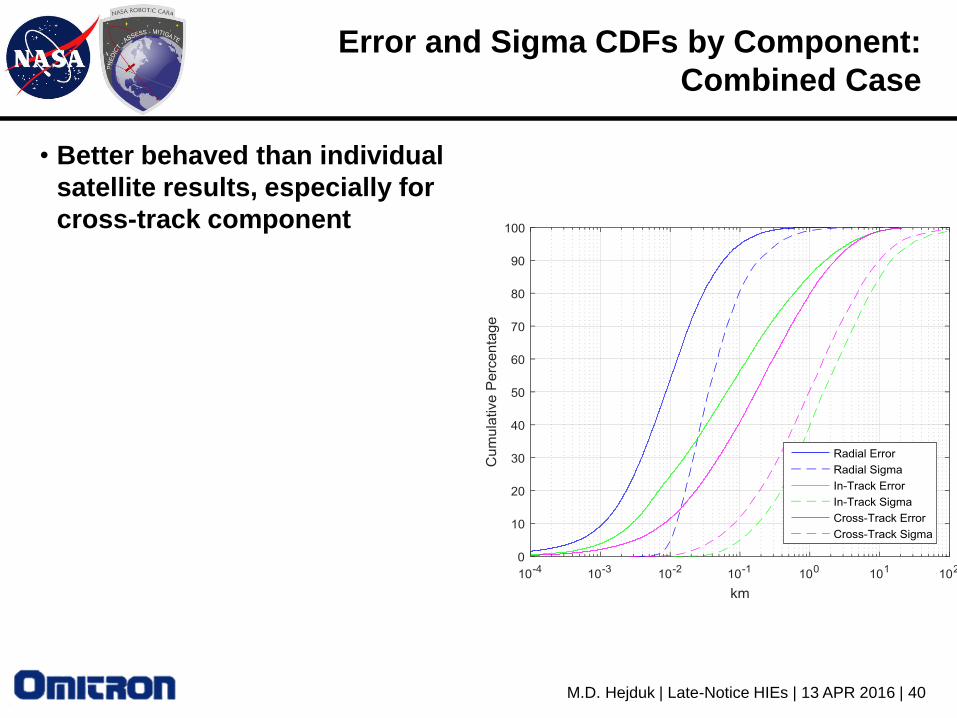
Error and Sigma CDFs by Component:
Combined Case
• Better behaved than individual
satellite results, especially for
cross-track component
M.D. Hejduk | Late-Notice HIEs | 13 APR 2016 | 41
CORRELATION INVESTIGATIONS
Combined Situation

M.D. Hejduk | Late-Notice HIEs | 13 APR 2016 | 42
Positive Change in Pc vs ε/σ
M.D. Hejduk | Late-Notice HIEs | 13 APR 2016 | 43
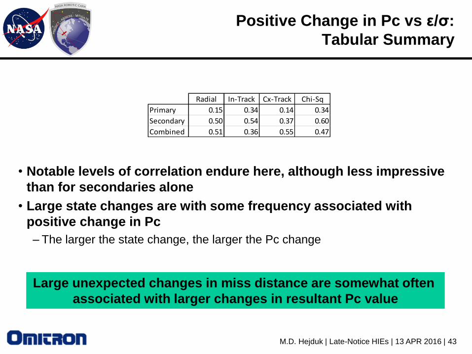
Positive Change in Pc vs ε/σ:
Tabular Summary
• Notable levels of correlation endure here, although less impressive
than for secondaries alone
• Large state changes are with some frequency associated with
positive change in Pc
– The larger the state change, the larger the Pc change
Radial In-Track Cx-Track Chi-Sq
Primary 0.15 0.34 0.14 0.34
Secondary 0.50 0.54 0.37 0.60
Combined 0.51 0.36 0.55 0.47
Large unexpected changes in miss distance are somewhat often
associated with larger changes in resultant Pc value
M.D. Hejduk | Late-Notice HIEs | 13 APR 2016 | 44
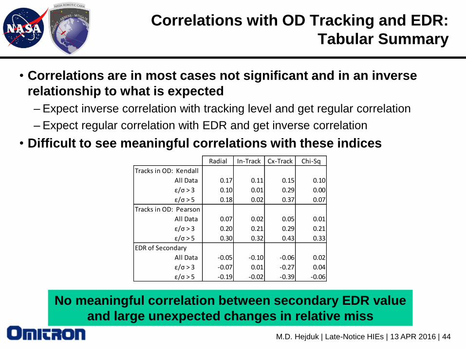
Correlations with OD Tracking and EDR:
Tabular Summary
• Correlations are in most cases not significant and in an inverse
relationship to what is expected
– Expect inverse correlation with tracking level and get regular correlation
– Expect regular correlation with EDR and get inverse correlation
• Difficult to see meaningful correlations with these indices
Radial In-Track Cx-Track Chi-Sq
Tracks in OD: Kendall
All Data 0.17 0.11 0.15 0.10
ε/σ > 3 0.10 0.01 0.29 0.00
ε/σ > 5 0.18 0.02 0.37 0.07
Tracks in OD: Pearson
All Data 0.07 0.02 0.05 0.01
ε/σ > 3 0.20 0.21 0.29 0.21
ε/σ > 5 0.30 0.32 0.43 0.33
EDR of Secondary
All Data -0.05 -0.10 -0.06 0.02
ε/σ > 3 -0.07 0.01 -0.27 0.04
ε/σ > 5 -0.19 -0.02 -0.39 -0.06
No meaningful correlation between secondary EDR value
and large unexpected changes in relative miss

M.D. Hejduk | Late-Notice HIEs | 13 APR 2016 | 45
Correlations with Solar Activity
• Elevated levels of solar activity can produce an unstable
atmosphere whose density is difficult to model
– More strongly true with geomagnetic storms (Dst, Ap)
– Can also be observed with EUV (F10, M10, S10, Y10, &c.)
• Different possibilities for essence of the problem
– Higher solar activity simpliciter
– Mismatch between predicted and realized solar activity
• Will investigate the former with correlation studies
– Median F10 and Ap over prediction interval
– Peak Ap over prediction interval
• Will investigate the latter with case studies

M.D. Hejduk | Late-Notice HIEs | 13 APR 2016 | 46
Combined ε/σ vs Median F10:
All Data
M.D. Hejduk | Late-Notice HIEs | 13 APR 2016 | 47
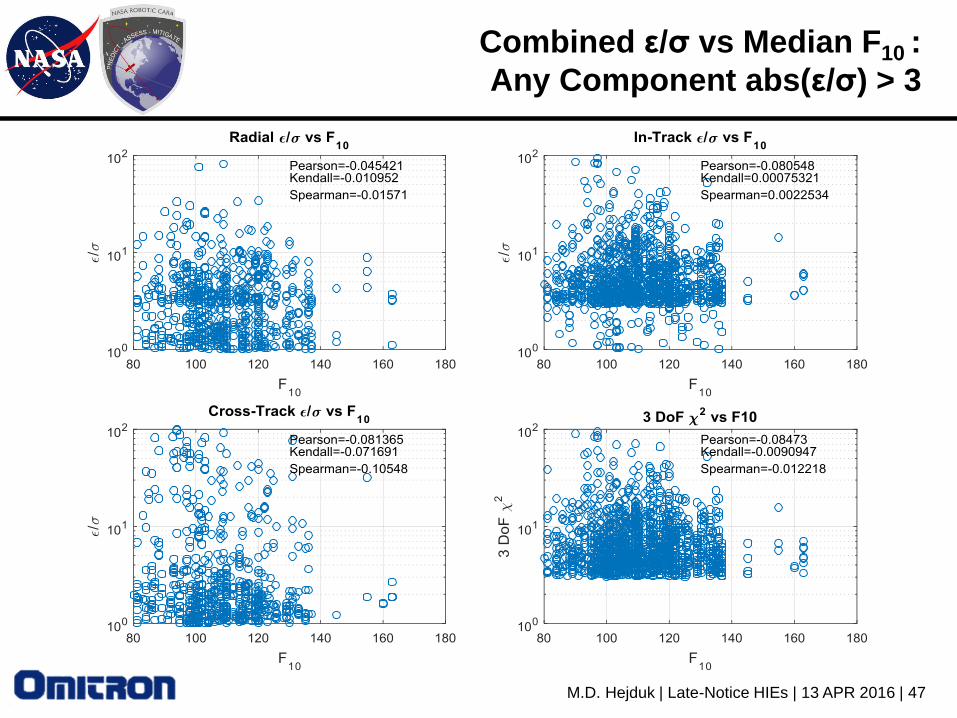
Combined ε/σ vs Median F10 :
Any Component abs(ε/σ) > 3
M.D. Hejduk | Late-Notice HIEs | 13 APR 2016 | 48
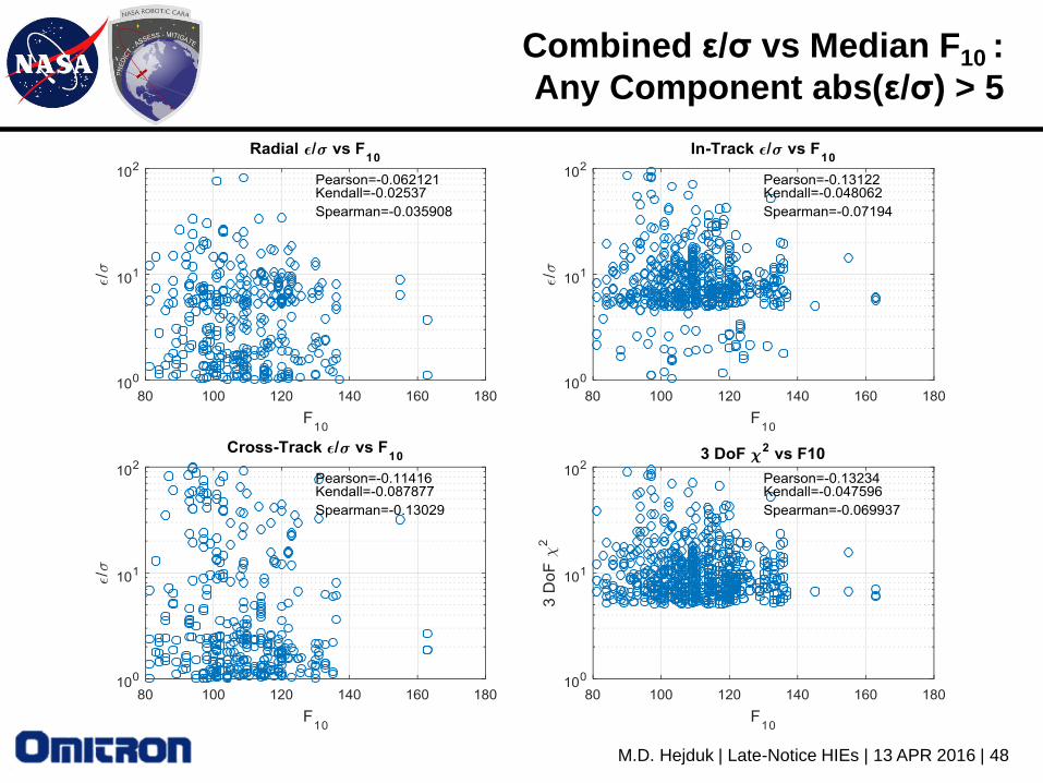
Combined ε/σ vs Median F10 :
Any Component abs(ε/σ) > 5
M.D. Hejduk | Late-Notice HIEs | 13 APR 2016 | 49
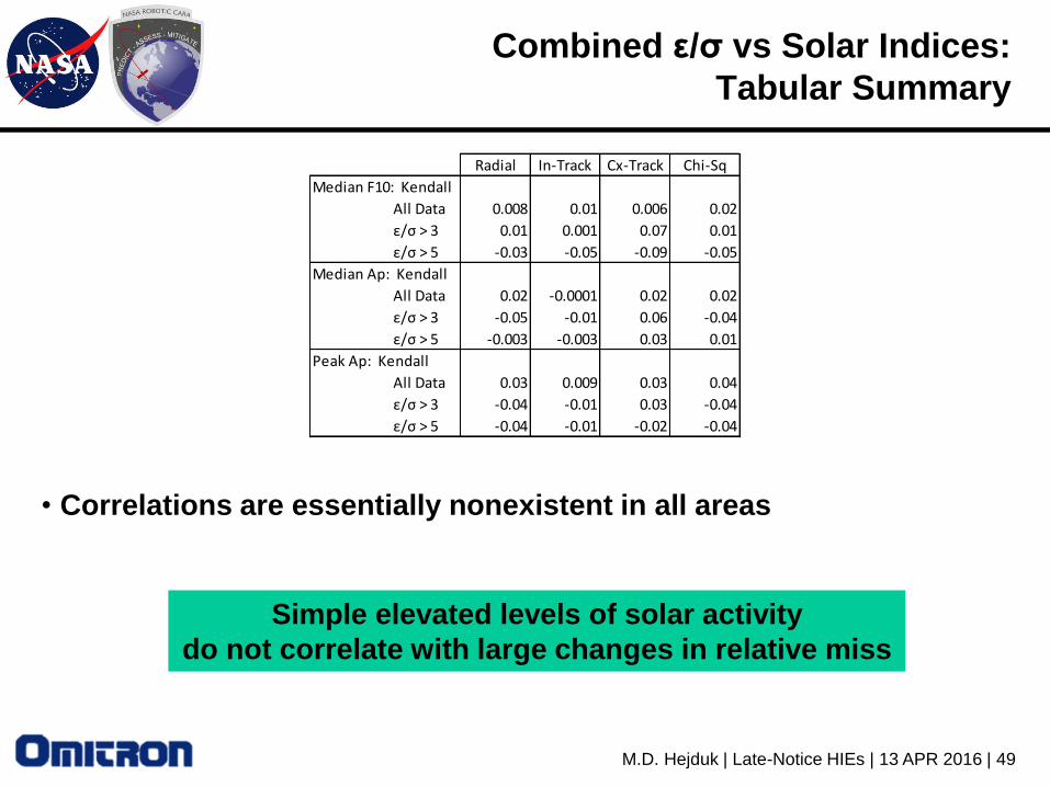
Combined ε/σ vs Solar Indices:
Tabular Summary
• Correlations are essentially nonexistent in all areas
Radial In-Track Cx-Track Chi-Sq
Median F10: Kendall
All Data 0.008 0.01 0.006 0.02
ε/σ > 3 0.01 0.001 0.07 0.01
ε/σ > 5 -0.03 -0.05 -0.09 -0.05
Median Ap: Kendall
All Data 0.02 -0.0001 0.02 0.02
ε/σ > 3 -0.05 -0.01 0.06 -0.04
ε/σ > 5 -0.003 -0.003 0.03 0.01
Peak Ap: Kendall
All Data 0.03 0.009 0.03 0.04
ε/σ > 3 -0.04 -0.01 0.03 -0.04
ε/σ > 5 -0.04 -0.01 -0.02 -0.04
Simple elevated levels of solar activity
do not correlate with large changes in relative miss
M.D. Hejduk | Late-Notice HIEs | 13 APR 2016 | 50
CASE STUDIES

M.D. Hejduk | Late-Notice HIEs | 13 APR 2016 | 51
Late-Notice HIE Case Studies
• Examined four late-notice events that fell within data investigation
period of current study
– 1 MAY 2015 to 1 FEB 2016
• Events examined
– Terra vs 38192, TCA 24 JUN 201
– Aura vs 89477; TCA 29 AUG 2015
– Terra vs 37131; TCA 19 DEC 2015
– GPM vs 28685; TCA 5 SEP 2015
• Will look at
– ε/σ vs time (same as Δ position to uncertainty
plots from daily/HIE report, like at right)
– Pc vs time (same as from daily/HIE report)
– Dst and Ap; prediction vs actual
• Segmented by what is available in support
of each update

M.D. Hejduk | Late-Notice HIEs | 13 APR 2016 | 52
JSpOC Space Weather Information Files:
Delivery Information
• Calculated externally at two different
sites, through an arrangement with
SET
• Forwarded three times a day to JSpOC
• Nominally at 0600, 1500, and 2100 Zulu
• Delivery goals met most of the time,
but not always
– Occasionally files late or missing, as shown
in graph at right
– 4.7% of file spacings deviate from nominal
cadence of 9 hrs, 9 hrs, and 6 hrs
M.D. Hejduk | Late-Notice HIEs | 13 APR 2016 | 53
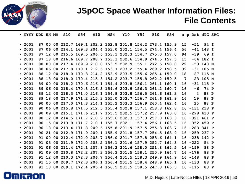
JSpOC Space Weather Information Files:
File Contents
• YYYY DDD HH MM S10 S54 M10 M54 Y10 Y54 F10 F54 a_p Dst dTC SRC
• 2001 87 00 00 212.7 169.1 202.2 152.8 201.8 154.2 273.4 155.9 15 -51 94 I
• 2001 87 06 00 214.1 169.3 204.4 153.0 202.1 154.5 274.4 156.4 56 -41 148 I
• 2001 87 12 00 215.5 169.5 206.6 153.1 202.3 154.7 275.0 157.0 94 -39 69 I
• 2001 87 18 00 216.6 169.7 208.7 153.3 202.6 154.9 274.5 157.5 15 -64 182 I
• 2001 88 00 00 217.4 169.9 210.8 153.5 202.9 155.1 272.5 158.0 22 -53 148 N
• 2001 88 06 00 217.8 170.1 212.6 153.7 203.2 155.4 269.2 158.5 39 -31 105 N
• 2001 88 12 00 218.0 170.3 214.2 153.9 203.5 155.6 265.4 159.0 18 -27 115 N
• 2001 88 18 00 218.0 170.4 215.3 154.2 203.7 155.8 262.2 159.5 7 -23 105 N
• 2001 89 00 00 218.2 170.6 216.1 154.4 203.8 156.1 261.1 160.1 16 -31 115 P
• 2001 89 06 00 218.4 170.8 216.3 154.6 203.9 156.3 261.2 160.7 16 -6 74 P
• 2001 89 12 00 218.3 171.0 216.1 154.8 203.8 156.5 261.6 161.3 16 4 88 P
• 2001 89 18 00 217.9 171.2 215.3 155.0 203.7 156.7 261.6 161.9 16 19 88 P
• 2001 90 00 00 217.0 171.3 214.1 155.2 203.3 156.9 260.4 162.4 16 35 88 P
• 2001 90 06 00 215.8 171.5 212.5 155.4 202.8 157.1 258.8 162.8 16 -131 218 P
• 2001 90 09 00 215.1 171.6 211.7 155.5 202.5 157.2 257.9 163.0 16 -298 410 P
• 2001 90 12 00 214.5 171.7 210.9 155.6 202.3 157.3 257.0 163.3 16 -321 461 P
• 2001 90 15 00 213.9 171.7 210.1 155.7 202.1 157.4 256.1 163.5 16 -352 459 P
• 2001 90 18 00 213.4 171.8 209.6 155.8 201.9 157.5 255.3 163.7 16 -283 341 P
• 2001 90 21 00 212.9 171.9 209.1 155.9 201.8 157.7 254.5 163.9 16 -259 237 P
• 2001 91 00 00 212.4 172.0 208.7 156.0 201.7 157.8 253.6 164.1 16 -238 142 P
• 2001 91 03 00 211.9 172.0 208.2 156.1 201.6 157.9 252.7 164.3 16 -222 54 P
• 2001 91 06 00 211.4 172.1 207.8 156.2 201.6 158.0 251.8 164.5 16 -199 88 P
• 2001 91 09 00 210.8 172.2 207.3 156.3 201.5 158.1 250.9 164.7 16 -176 88 P
• 2001 91 12 00 210.3 172.3 206.7 156.4 201.5 158.3 249.9 164.9 16 -148 88 P
• 2001 91 15 00 209.7 172.3 206.1 156.4 201.5 158.4 248.9 165.1 16 -133 88 P
• 2001 91 18 00 209.1 172.4 205.4 156.5 201.5 158.5 247.8 165.3 16 -115 88 P

M.D. Hejduk | Late-Notice HIEs | 13 APR 2016 | 54
JSpOC Space Weather Information Files:
Data Currency
• Three types of data in file
– “Issued” – definitive values for the solar/geomagnetic index, subjected to full
availability of feeder data and consistency tests
– “Nowcast” – initial observations of values, hand-scaled and not subject to
consistency tests
• Measurements stay in “nowcast” status for typically 24 hours
– “Predicted” – values are predicted
• EUV predicted values from 54- and sometimes 108-day autoregression analyses of
past data
• Geomagnetic indices are predicted from observed solar activity earlier in the solar
rotation (and thus expected to become georelevant at a given future time)
• Data type timing
– Issued/Nowcast data used in propagating states from epoch to current time
• Scaled/debiased with HASDM results
– Predicted data used in propagating states from current time to TCA
– Accuracy of predicted data can influence propagated result substantially
M.D. Hejduk | Late-Notice HIEs | 13 APR 2016 | 55
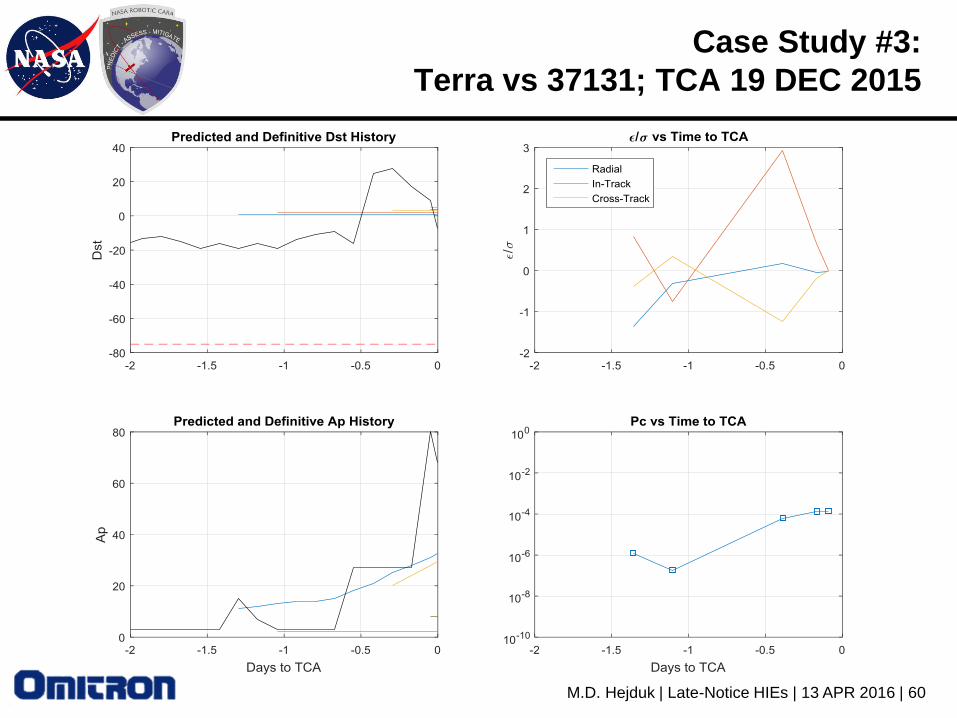
Space Weather Evolution Charts
• Upper left shows Dst; lower left shows Ap
• Black line is “issued” (definitive) data
• Colored lines are predicted data
– Each line begins when a given OD update executed
– Each line shows predicted values of the geomagnetic index of choice
• When Dst lines move to small positive value, prediction stops (zeroes in file)
• When Ap lines move to small negative value, prediction stops (ones in file)
• Dst threshold for solar storm compensation engagement also shown
• Upper right shows ε/σ for each component
– Miss distance vs combined covariance
• Lower right shows Pc vs time

M.D. Hejduk | Late-Notice HIEs | 13 APR 2016 | 56
Case Study #1:
Terra vs 38192, TCA 24 JUN 2015

M.D. Hejduk | Late-Notice HIEs | 13 APR 2016 | 57
Space Weather Trade-Space Result:
61 Hours to TCA
• About half a day before spike in
Ap/Dst begins
– Some predicted increased Dst
activity, but not of severity actually
realized
– Predictions at very end of storm
over-predict Dst
– Final prediction and shrinking
covariance produces Pc dropoff
• SWTS indicates conjunction
vulnerable to large Pc changes
due to density mismodeling
• Bottom line: missed solar storm
and subsequent prediction
failures produced late changes

M.D. Hejduk | Late-Notice HIEs | 13 APR 2016 | 58
Case Study #2:
Aura vs 89477; TCA 29 AUG 2015
M.D. Hejduk | Late-Notice HIEs | 13 APR 2016 | 59
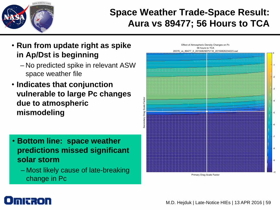
Space Weather Trade-Space Result:
Aura vs 89477; 56 Hours to TCA
• Run from update right as spike
in Ap/Dst is beginning
– No predicted spike in relevant ASW
space weather file
• Indicates that conjunction
vulnerable to large Pc changes
due to atmospheric
mismodeling
• Bottom line: space weather
predictions missed significant
solar storm
– Most likely cause of late-breaking
change in Pc
M.D. Hejduk | Late-Notice HIEs | 13 APR 2016 | 60
Case Study #3:
Terra vs 37131; TCA 19 DEC 2015
M.D. Hejduk | Late-Notice HIEs | 13 APR 2016 | 61
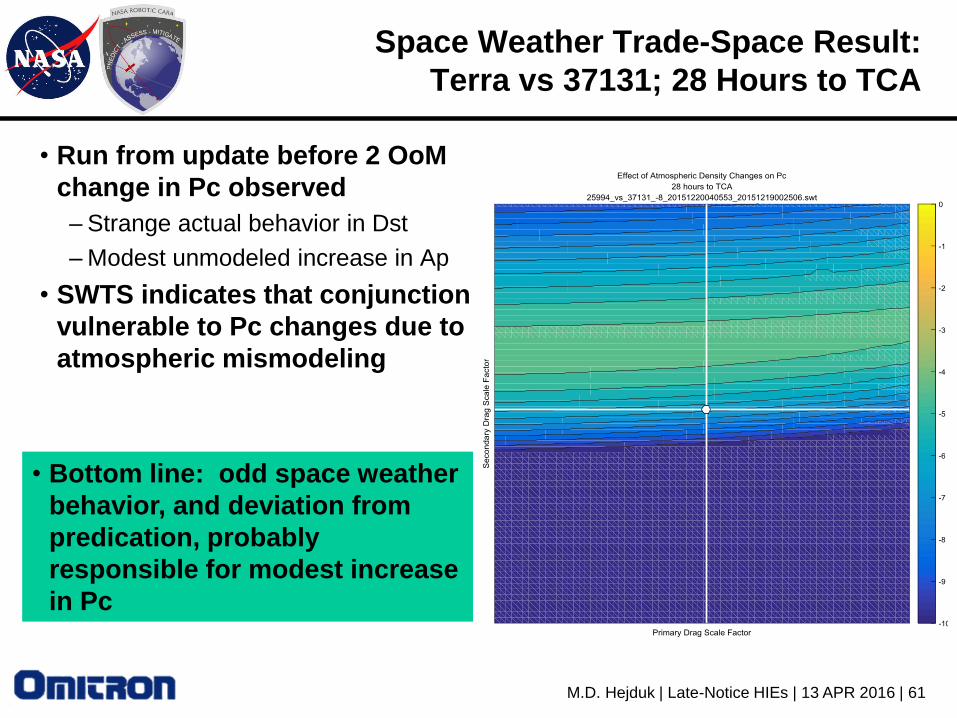
Space Weather Trade-Space Result:
Terra vs 37131; 28 Hours to TCA
• Run from update before 2 OoM
change in Pc observed
– Strange actual behavior in Dst
– Modest unmodeled increase in Ap
• SWTS indicates that conjunction
vulnerable to Pc changes due to
atmospheric mismodeling
• Bottom line: odd space weather
behavior, and deviation from
predication, probably
responsible for modest increase
in Pc

M.D. Hejduk | Late-Notice HIEs | 13 APR 2016 | 62
Case Study #4:
GPM vs 28685; TCA 5 SEP 2015
M.D. Hejduk | Late-Notice HIEs | 13 APR 2016 | 63
Case Study #4:
Situation
• No particular space weather anomalies here
• Rather, simply a late-notice event
• When did this event first appear in the screenings?
– Because of ongoing screening-volume study, results from “large screening”
experiment available during this period
• 50 x 250 x 250
– Can see how object fared against operational screening volume

M.D. Hejduk | Late-Notice HIEs | 13 APR 2016 | 64
Case Study #4:
Screening Results (TCA on 09/05)
M.D. Hejduk | Late-Notice HIEs | 13 APR 2016 | 65
Case Study #4:
Screening Results Discussion
• Late-notice situation here mostly bad luck
– R and C components within screening volume ~6 days before TCA
– In-track component above threshold for several days, barely above threshold
two days before TCA, and violates it about 17 hours before TCA
– CDM appears to have been generated as part of run subsequent to screening
• Increased speed of current processes will improve this situation
somewhat in future
– 3 screenings/day will find such edge cases faster
– Faster processing will get CDM out faster after conjunction discovery
M.D. Hejduk | Late-Notice HIEs | 13 APR 2016 | 66
SUMMARY AND WAY FORWARD
M.D. Hejduk | Late-Notice HIEs | 13 APR 2016 | 67
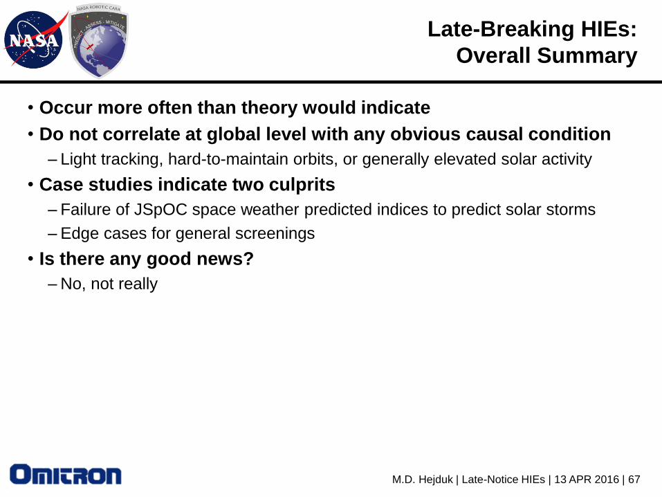
Late-Breaking HIEs:
Overall Summary
• Occur more often than theory would indicate
• Do not correlate at global level with any obvious causal condition
– Light tracking, hard-to-maintain orbits, or generally elevated solar activity
• Case studies indicate two culprits
– Failure of JSpOC space weather predicted indices to predict solar storms
– Edge cases for general screenings
• Is there any good news?
– No, not really

M.D. Hejduk | Late-Notice HIEs | 13 APR 2016 | 68
Solar Storm Predictions:
What are we Doing? (1 of 2)
• CARA member of NASA LWS space weather expert panel
– Dr. Matt Hejduk as CA expert panel representative
– Dr. Yihua Zheng as GSFC space physics representative, also representing
mission interests
• Purpose of panel to recommend NASA research investments to
improve prediction and modeling
– Will issue formal report of recommendations by December, as well as
accompanying journal article
– Will attempt to focus at least part of recommendation to address JSpOC
situation
• Hope to leverage report to push state of the art at JSpOC
– However, from their perspective, a large investment was just made in
atmospheric density prediction modeling; need to focus on other items

M.D. Hejduk | Late-Notice HIEs | 13 APR 2016 | 69
Solar Storm Predictions:
What are we Doing? (2 of 2)
• Will investigate whether file update frequency can be accelerated
– Brief JSpOC on these results to show the problems that latencies create
• See if there are mechanisms to improve efficiencies
– Use SWTS function to determine whether such intervention is needed
• Events that are not vulnerable to atmospheric density mismodeling would not require
out-of-cycle updates
– Would not have helped cases investigated here, as entire solar storms were
missed
• However, probably a fairly long time before there is much
improvement with such scenarios

M.D. Hejduk | Late-Notice HIEs | 13 APR 2016 | 70
Screening Volume Sizing:
What are we Doing?
• First, must recognize that edge cases will exist with any volume size
• Study of proper screening volume sizing presently in work
– Preliminary results set briefed to JSpOC in March
– Set of refinements presently being performed; expect to issue a definitive
update in next couple of months
• Certain philosophical issues need to be adjudicated
– e.g., increasing screening volume size to produce a large number of additional
events, all with a Pc of 0, does nothing to provide better situational awareness
• In the end, two changes will probably take place
– Screening volume sizes will increase
– Some sort of additional winnowing test on captured candidates will be
performed in order to identify events worthy of increased attention/tasking
• Stay tuned!

N. Sabey | ERB | 18 Jun 2013 | 71
BACKUP SLIDES
M.D. Hejduk | Late-Notice HIEs | 13 APR 2016 | 72
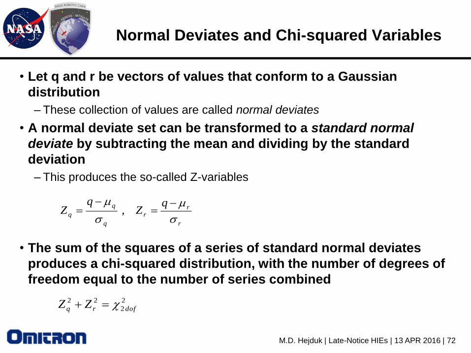
Normal Deviates and Chi-squared Variables
• Let q and r be vectors of values that conform to a Gaussian
distribution
– These collection of values are called normal deviates
• A normal deviate set can be transformed to a standard normal
deviate by subtracting the mean and dividing by the standard
deviation
– This produces the so-called Z-variables
• The sum of the squares of a series of standard normal deviates
produces a chi-squared distribution, with the number of degrees of
freedom equal to the number of series combined
r
rr
q
q
q
qZ
qZ
,
2
2
22
dofrq ZZ
M.D. Hejduk | Late-Notice HIEs | 13 APR 2016 | 73
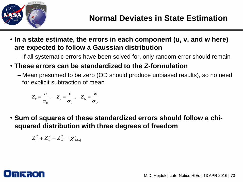
Normal Deviates in State Estimation
• In a state estimate, the errors in each component (u, v, and w here)
are expected to follow a Gaussian distribution
– If all systematic errors have been solved for, only random error should remain
• These errors can be standardized to the Z-formulation
– Mean presumed to be zero (OD should produce unbiased results), so no need
for explicit subtraction of mean
• Sum of squares of these standardized errors should follow a chi-
squared distribution with three degrees of freedom
w
w
v
v
u
u
wZ
vZ
uZ
,,
2
3
222
dofwvu ZZZ

M.D. Hejduk | Late-Notice HIEs | 13 APR 2016 | 74
State Estimation Example Calculation
• Let us presume we have a precision ephemeris, state estimate, and
covariance about the state estimate
– For the present, further presume covariance aligns perfectly with uvw frame
(no off-diagonal terms)
• Error vector ε is position difference between state estimate and
precision ephemeris, and covariance consists only of variances
along the diagonal
– Inverse of covariance matrix is straightforward
• Resultant simple formula for chi-squared variables
• Extension to case with off-diagonal terms straightforward
2
2
2
00
00
00
,
w
v
u
w
v
u
C
2
2
2
1
100
010
001
w
v
u
C
2
32
2
2
2
2
21
dof
w
u
v
v
u
uTC


