
Orbital Mechanics!Space System Design, MAE 342, Princeton University!
Robert Stengel
Copyright 2016 by Robert Stengel. All rights reserved. For educational use only.http://www.princeton.edu/~stengel/MAE342.html
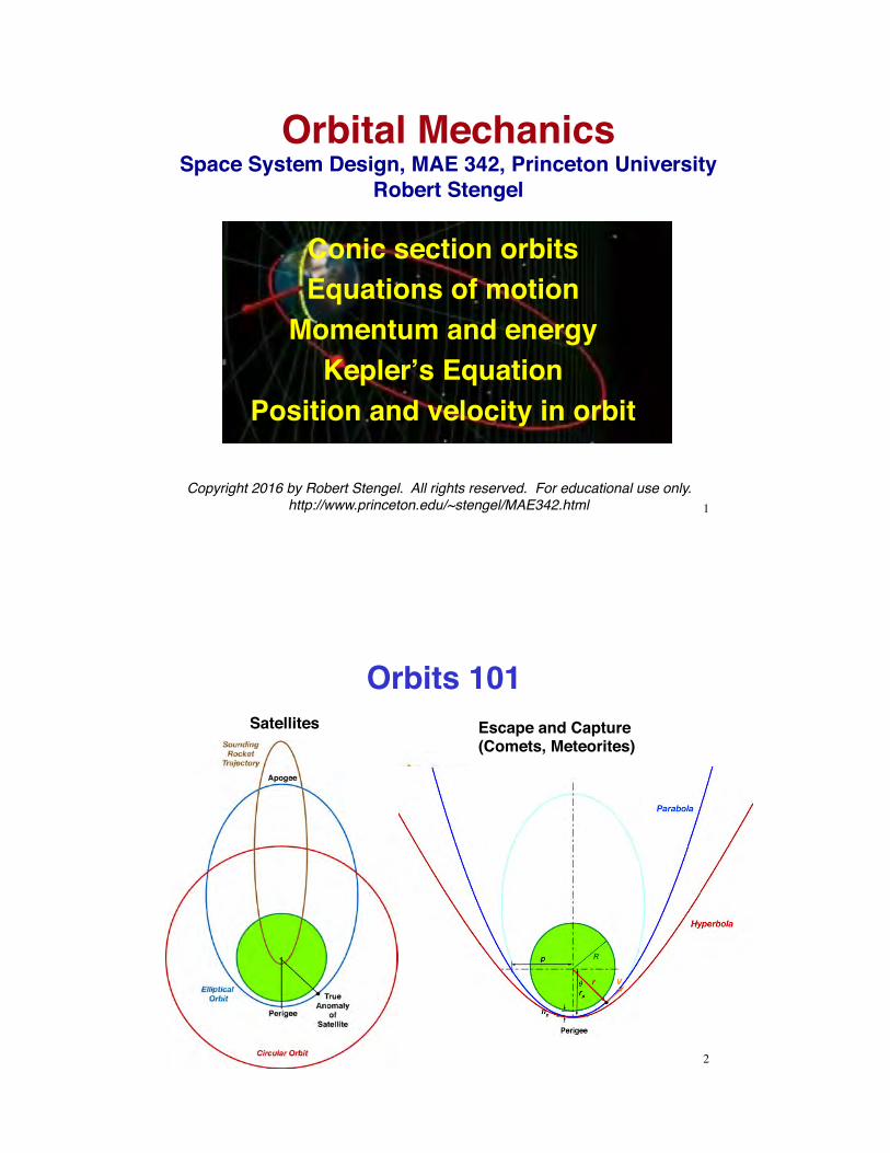
Conic section orbitsEquations of motion
Momentum and energyKepler’s Equation
Position and velocity in orbit
1
Orbits 101 Satellites Escape and Capture
(Comets, Meteorites)
2

Two-Body Orbits are Conic Sections
3
Classical Orbital ElementsDimension and Time
Orientation
a : Semi-major axise : Eccentricity
t p: Time of perigee passage
! :Longitude of the Ascending/Descending Nodei : Inclination of the Orbital Plane
" : Argument of Perigee
4
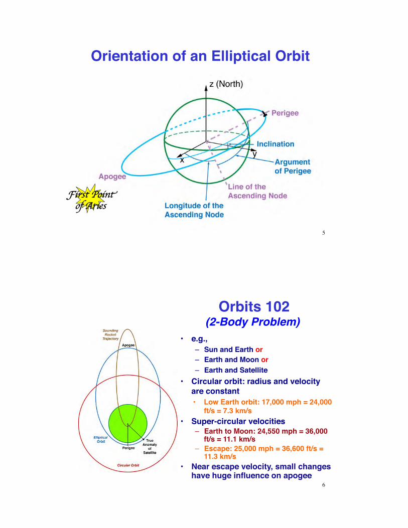
Orientation of an Elliptical Orbit
5
!!iirrsstt PPooiinn"" ooff AArriieess
Orbits 102(2-Body Problem)
•! e.g., –! Sun and Earth or–! Earth and Moon or–! Earth and Satellite
•! Circular orbit: radius and velocity are constant•! Low Earth orbit: 17,000 mph = 24,000
ft/s = 7.3 km/s•! Super-circular velocities
–! Earth to Moon: 24,550 mph = 36,000 ft/s = 11.1 km/s
–! Escape: 25,000 mph = 36,600 ft/s = 11.3 km/s
•! Near escape velocity, small changes have huge influence on apogee
6

!! Particle of fixed mass (also called a point mass) acted upon by a force changes velocity with !! acceleration proportional to and in direction of force
!! Inertial reference frame !! Ratio of force to acceleration is the mass of the
particle: F = m a
Newton’s 2nd Law
ddt
mv t( )!" #$ = mdv t( )dt
= ma t( ) = F
F =
fxfyfz
!
"
%%%%
#
$
&&&&
= force vectorm ddt
vx t( )vy t( )vz t( )
!
"
####
$
%
&&&&
=
fxfyfz
!
"
####
$
%
&&&&
7
Equations of Motion for a Particle
dv t( )dt
= !v t( ) = 1mF =
fx mfy m
fz m
!
"
####
$
%
&&&&
=
axayaz
!
"
####
$
%
&&&&
Integrating the acceleration (Newton’s 2nd Law) allows us to solve for the velocity of the particle
v T( ) = dv t( )dt
dt0
T
! + v 0( ) = a t( )dt0
T
! + v 0( ) = 1mFdt
0
T
! + v 0( )
vx T( )vy T( )vz T( )
!
"
####
$
%
&&&&
=
ax t( )ay t( )az t( )
!
"
####
$
%
&&&&
dt0
T
' +
vx 0( )vy 0( )vz 0( )
!
"
####
$
%
&&&&
=
fx t( ) mfy t( ) mfz t( ) m
!
"
####
$
%
&&&&
dt0
T
' +
vx 0( )vy 0( )vz 0( )
!
"
####
$
%
&&&&
3 components of velocity
8

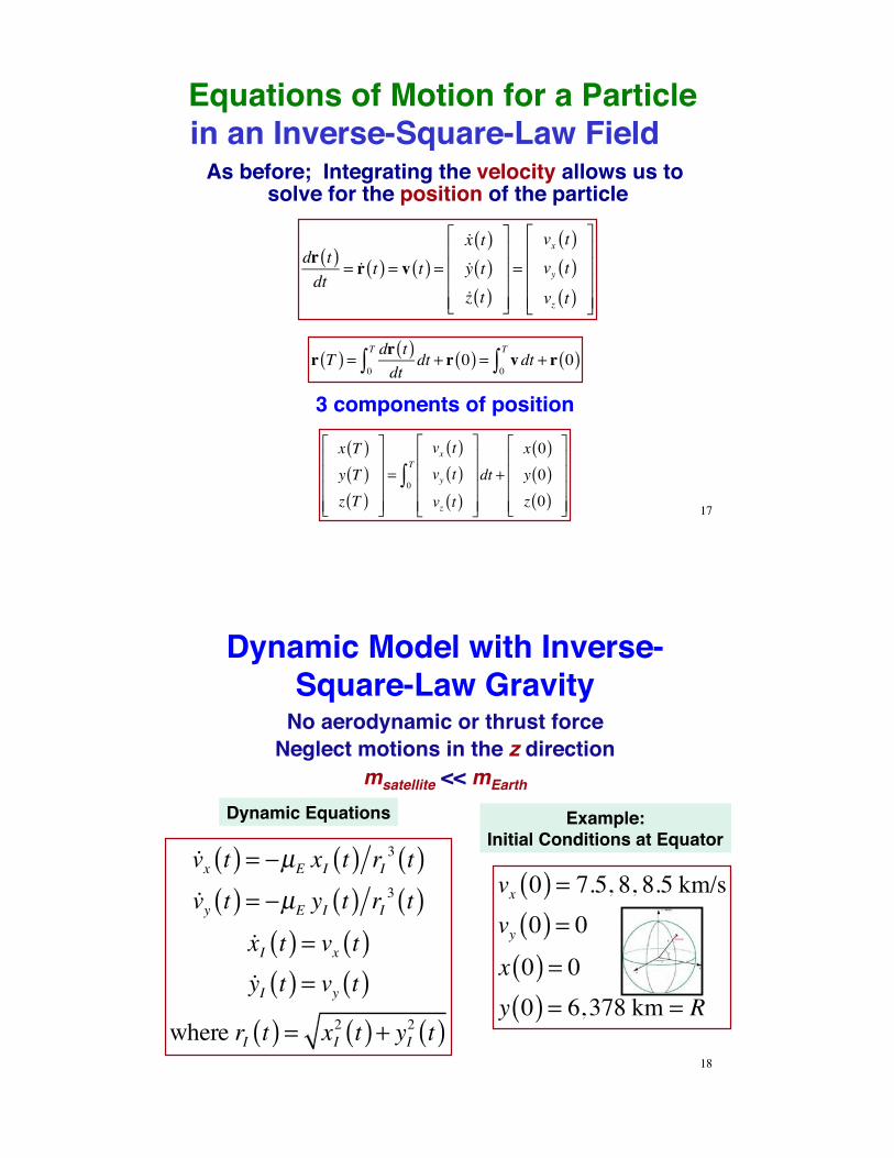
Equations of Motion for a Particle
dr t( )dt
= !r t( ) = v t( ) =!x t( )!y t( )!z t( )
!
"
####
$
%
&&&&
=
vx t( )vy t( )vz t( )
!
"
####
$
%
&&&&
Integrating the velocity allows us to solve for the position of the particle
r T( ) = dr t( )dt
dt0
T
! + r 0( ) = vdt0
T
! + r 0( )
x T( )y T( )z T( )
!
"
####
$
%
&&&&
=
vx t( )vy t( )vz t( )
!
"
####
$
%
&&&&
dt0
T
' +
x 0( )y 0( )z 0( )
!
"
####
$
%
&&&&
3 components of position
9
Spherical Model of the Rotating Earth
RE =xoyozo
!
"
###
$
%
&&&E
=cosLE cos'E
cosLE sin'E
sinLE
!
"
###
$
%
&&&R
Spherical model of earth s surface, earth-fixed (rotating) coordinates
LE : Latitude (from Equator), deg!E : Longitude (from Prime Meridian), degR : Radius (from Earth's center), deg
Earth's rotation rate, ! , is 15.04 deg/hr10

Non-Rotating (Inertial) Reference Frame for the Earth
Celestial longitude, !C, measured from First Point of Aries on the
Celestial Sphere at Vernal Equinox
!C = !E +" t # tepoch( ) = !E +" $t
11
Transformation Effects of Rotation
RE =cos!"t sin!"t 0#sin!"t cos!"t 0
0 0 1
$
%
&&&
'
(
)))R I =
cos!"t sin!"t 0#sin!"t cos!"t 0
0 0 1
$
%
&&&
'
(
)))
xoyozo
$
%
&&&
'
(
)))I
rE =cosLE cos!E
cosLE sin!E
sinLE
"
#
$$$
%
&
'''R + Altitude( ); rI =
cosLE cos!CcosLE sin!CsinLE
"
#
$$$
%
&
'''R + Altitude( )
Transformation from inertial frame, I, to Earth’s rotating frame, E
Location of satellite, rotating and inertial frames
Orbital calculations generally are made in an inertial frame of reference
12
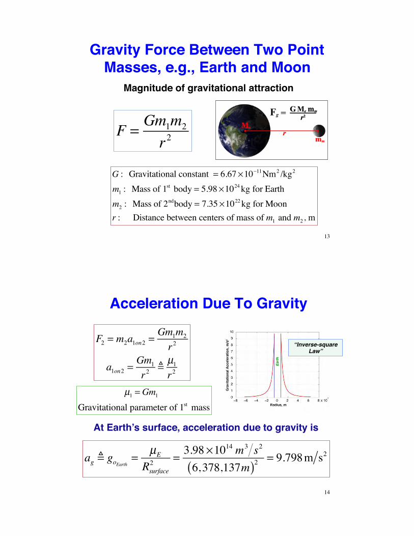
Gravity Force Between Two Point Masses, e.g., Earth and Moon
Magnitude of gravitational attraction
G : Gravitational constant = 6.67 !10"11Nm2 /kg2
m1 : Mass of 1st body = 5.98 !1024 kg for Earthm2 : Mass of 2ndbody = 7.35 !1022 kg for Moonr : Distance between centers of mass of m1 and m2, m
F = Gm1m2
r2
13
Acceleration Due To Gravity
F2 = m2a1on2 =Gm1m2
r2
a1on2 =Gm1
r2!µ1r2
At Earth’s surface, acceleration due to gravity is
ag ! goEarth =
µE
Rsurface2 = 3.98 !10
14 m3 s2
6,378,137m( )2= 9.798m s2
µ1 = Gm1 Gravitational parameter of 1st mass
14
“Inverse-square Law”

Gravitational Force Vector of the Spherical Earth
Force always directed toward the Earth’s center
rIrI
=
xyz
!
"
###
$
%
&&&I
xI2 + yI
2 + zI2=
cosLE cos'I
cosLE sin'I
sinLE
!
"
###
$
%
&&&
Fg = !m µE
rI2rIrI
"
#$%
&'= !m µE
rI3
xyz
(
)
***
+
,
---I
(vector), as rI = rI
(x, y, z) establishes the direction of the local vertical
15
Equations of Motion for a Particle in an Inverse-Square-Law Field
dv t( )dt
= !v t( ) = 1mFg = ! µE
rI2rIrI
"
#$%
&'= ! µE
rI3
xyz
(
)
***
+
,
---
Integrating the acceleration (Newton’s 2nd Law) allows us to solve for the velocity of the particle
v T( ) = dv t( )dt
dt0
T
! + v 0( ) = a t( )dt0
T
! + v 0( ) = 1mFdt
0
T
! + v 0( )
vx T( )vy T( )vz T( )
!
"
####
$
%
&&&&
= 'µE
x rI3
y rI3
z rI3
!
"
####
$
%
&&&&
dt0
T
( +
vx 0( )vy 0( )vz 0( )
!
"
####
$
%
&&&&
3 components of velocity
16
Equations of Motion for a Particle in an Inverse-Square-Law Field
dr t( )dt
= !r t( ) = v t( ) =!x t( )!y t( )!z t( )
!
"
####
$
%
&&&&
=
vx t( )vy t( )vz t( )
!
"
####
$
%
&&&&
As before; Integrating the velocity allows us to solve for the position of the particle
r T( ) = dr t( )dt
dt0
T
! + r 0( ) = vdt0
T
! + r 0( )
x T( )y T( )z T( )
!
"
####
$
%
&&&&
=
vx t( )vy t( )vz t( )
!
"
####
$
%
&&&&
dt0
T
' +
x 0( )y 0( )z 0( )
!
"
####
$
%
&&&&
3 components of position
17
Dynamic Model with Inverse-Square-Law Gravity
No aerodynamic or thrust forceNeglect motions in the z direction
msatellite << mEarth
!vx t( ) = !µE xI t( ) rI 3 t( )!vy t( ) = !µE yI t( ) rI 3 t( )
!xI t( ) = vx t( )!yI t( ) = vy t( )
where rI t( ) = xI2 t( ) + yI2 t( )
vx 0( ) = 7.5, 8, 8.5 km/svy 0( ) = 0x 0( ) = 0y 0( ) = 6,378 km = R
Dynamic Equations Example:Initial Conditions at Equator
18

19
Equatorial Orbits Calculated with Inverse-Square-Law Model
Work“Work” is a scalar measure of change in energy
With constant force,In one dimension
W12 = F r2 ! r1( ) = F"r
With varying force, work is the integral
W12 = FT drr1
r2
! = fxdx + fydy + fzdz( )r1
r2
! , dr =dxdydz
"
#
$$$
%
&
'''
In three dimensionsW12 = F
T r2 ! r1( ) = FT"r
20

Conservative Force!! Assume that the 3-D force
field is a function of position
F = F r( )
Iron FilingsAround Magnet
Force Emanating from Source
!! The force field is conservative if
FT r( )drr1
r2
! + FT r( )drr2
r1
! = 0
… for any path between r1 and r2 and back
21
Gravitational Force is Gradient of a Potential, V(r)
Gravity potential, V(r), is a function only of position
Fg = !m µE
rI3 rI =
""r
m µE
r#$%
&'(!
""rV r( )
22

Gravitational Force FieldGravitational force field
Gravitational force field is conservative because
… for any path between r1 and r2 and back
Fg = !m µE
rI3 rI
23
!!rV r( )drI
r1
r2
" # !!rV r( )drI
r2
r1
" =
# m µE
rI3 rI drI
r1
r2
" + m µE
rI3 rI drI
r1
r2
" = 0
Potential Energy in Gravitational Force Field
Potential energy, V or PE, is defined with respect to a reference point, r0
!PE !V r2( )"V r1( ) = " m µ
r2+V0
#$%
&'(+ m µ
r1+V0
#$%
&'(= "m µ
r2+m µ
r1
PE r0( ) =V r0( ) =V0 ! "U0( )
24
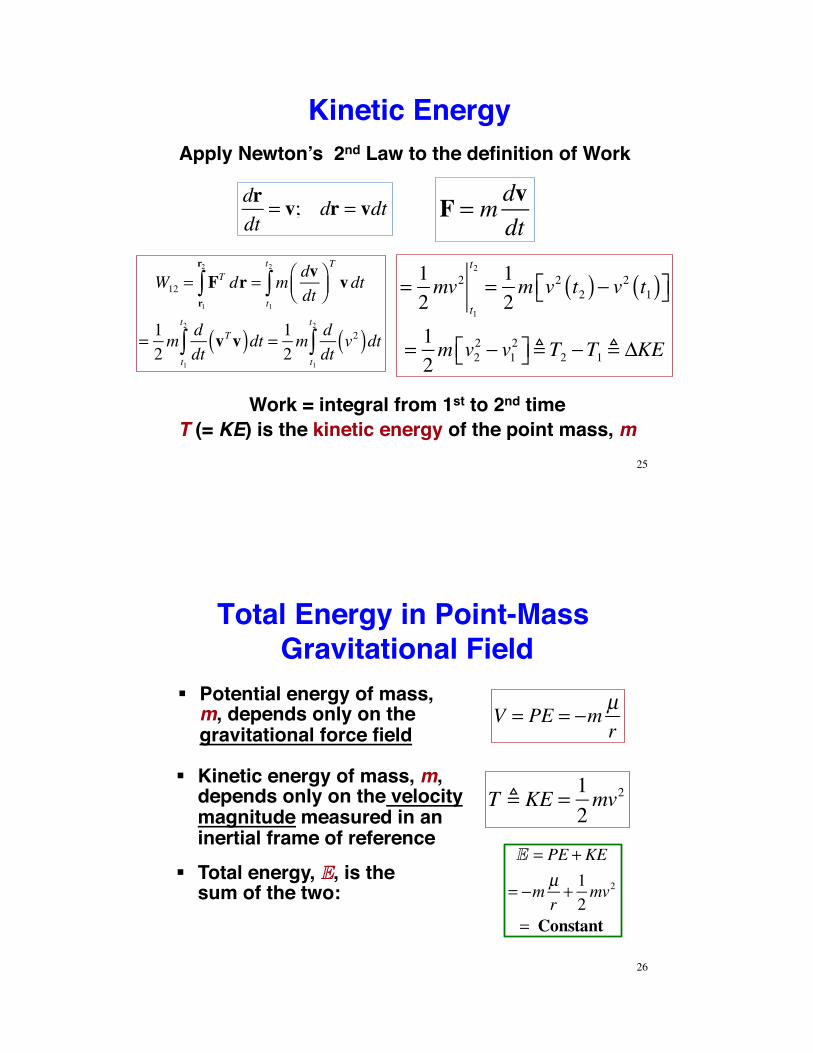
Kinetic EnergyApply Newton’s 2nd Law to the definition of Work
drdt
= v; dr = vdt F = m dvdt
W12 = FT drr1
r2
! = m dvdt
"#$
%&'T
vdtt1
t2
!
= 12m d
dtvTv( )dt
t1
t2
! = 12m d
dtv2( )dt
t1
t2
!
= 12mv2
t1
t2
= 12m v2 t2( )! v2 t1( )"# $%
= 12m v2
2 ! v12"# $% ! T2 !T1 ! &KE
Work = integral from 1st to 2nd timeT (= KE) is the kinetic energy of the point mass, m
25
Total Energy in Point-Mass Gravitational Field
!! Potential energy of mass, m, depends only on the gravitational force field
T ! KE = 1
2mv2
!! Total energy, E, is the sum of the two:
!! Kinetic energy of mass, m, depends only on the velocity magnitude measured in an inertial frame of reference
V = PE = !m µr
E = PE + KE
= !m µr+ 1
2mv2
= Constant
26

Interchange Between Potential and Kinetic Energy in a Conservative System
!m µr2+m µ
r1
"#$
%&'= 12mv2
2 ! 12mv1
2"#$
%&'
PE2 ! PE1 = KE2 ! KE1P1
P2
27
E 2 !E1 = 0
!m µr2+ 12mv2
2"#$
%&'! !m µ
r1+ 12mv1
2"#$
%&'= 0
Specific Energy…Energy per unit of the satellite’s mass
E S = PES + KES
= 1m
! mµr
+ 12mv2"
#$%&'
= ! µr+ 12v2
P1
P2
28
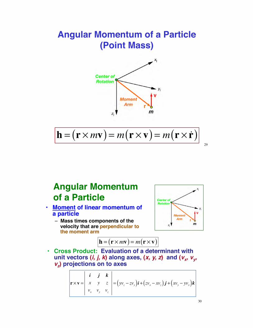
Angular Momentum of a Particle (Point Mass)
h = r !mv( ) = m r ! v( ) = m r ! !r( )29
Angular Momentum of a Particle
•! Moment of linear momentum of a particle–! Mass times components of the
velocity that are perpendicular to the moment arm
•! Cross Product: Evaluation of a determinant with unit vectors (i, j, k) along axes, (x, y, z) and (vx, vy, vz) projections on to axes
r ! v =i j kx y zvx vy vz
= yvz " zvy( )i + zvx " xvz( ) j + xvy " yvx( )k
h = r !mv( ) = m r ! v( )
30

Cross Product in Column Notation
r ! v =i j kx y zvx vy vz
= yvz " zvy( )i + zvx " xvz( ) j + xvy " yvx( )k
r ! v =
yvz " zvy( )zvx " xvz( )xvy " yvx( )
#
$
%%%%%
&
'
(((((
Column notation
Cross product identifies perpendicular components of r and v
31
=0 !z yz 0 !x!y x 0
"
#
$$$
%
&
'''
vxvyvz
"
#
$$$$
%
&
''''
Angular Momentum Vector is Perpendicular to Both Moment
Arm and Velocity
h = mr ! v = m
yvz " zvy( )zvx " xvz( )xvy " yvx( )
#
$
%%%%%
&
'
(((((
= m0 "z yz 0 "x"y x 0
#
$
%%%
&
'
(((
vxvyvz
#
$
%%%%
&
'
((((
= m!rv
32

Specific Angular Momentum Vector of a Satellite
hS =
mmr ! v = r ! v = r ! !r
… is the angular momentum per unit of the satellite’s mass, referenced to the center of attraction
Perpendicular to the orbital plane
33
Acceleration is
a t( ) = !v t( ) = !!r t( ) = ! µ
r2 t( )rI t( )r t( )
"
#$%
&'= ! µ
r3 t( ) r t( )
… or
!!r + µ
r3r = 0
Equations of Motion for a Particle in an Inverse-Square-Law Field
34

Cross Products of Radius and Radius Rate
Then
… because they are parallel
r ! !!r + µ
r3r"
#$%&'= 0
r ! r = 0 !r ! !r = 0
ddtr ! !r( ) = !r ! !r( ) + r ! !!r( ) = r ! !!r( )Chain Rule for Differentiation
35
Specific Angular Momentum
Consequently
r ! !!r + µ
r3r"
#$%&'= r ! !!r( ) + µ
r3r ! r( )
hS = Constant
hS ! h = r ! "r( ) (Perpendicular to the plane of motion)
Orbital plane is fixed in inertial space
= ddtr ! !r( ) = dhS
dt= 0
36
0

Eccentricity Vector is a Constant of Integration
With triple vector product identity (see Supplement)
!!r + µ
r3r!
"#$%&' h = !!r ' h+ µ
r3r ' h = 0
e = Eccentricity vector Constant of integration( )
!!r ! h = " µ
r3r ! h = " µ
r3r ! r ! !r( )
!!r ! h = " µ
r3r ! r ! !r( ) = " µ
r2!rr " r!r( ) = µ d
dtrr
#$%
&'(
Integrating
!!r ! h( )dt" = !r ! h = µ r
r+ e#
$%&'(
37
Significance of Eccentricity Vector
!r ! h" µ r
r+ e#
$%&'(
)*+
,-.
T
h = 0 because !r ! h" µ rr+ e#
$%&'(
)*+
,-.= 0
! !r " h( )T h# µrTh
r# µeTh = 0
!"µeTh = 0
0 0
!! e is perpendicular to angular momentum,
!! which means it lies in the orbital plane!! Its angle provides a reference direction
for the perigee38

General Polar Equation of a Conic Section
rT !r ! h" µ r
r+ e#
$%&'(
)*+
,-.= 0
39
1st term is angular momentum squared
rT !r ! h( ) = hT r ! !r( ) = hTh = h2
Then
h2 ! µ rTrr
+ rTe"#$
%&'= 0 h2 = µ r + rTe( ) = µ r + recos!( ) = 0
r = h2 µ1+ ecos!
r = p1+ e cos!
= h2 µ1+ e cos!
, m or km
! : True Anomaly =Angle from perigee direction, deg or rad
40
Elliptical Planetary Orbits!! Assume satellite mass is negligible
compared to Earth’s mass!! Then
!! Center of mass of the 2 bodies is at Earth’s center of mass
!! Center of mass is at one of ellipse’s focal points
!! Other focal point is “vacant”

Properties of Elliptical Orbits
e =ra ! rpra + rp
=ra ! rp2a
rp = a / 1! e( ) ra = a / 1+ e( )
a =ra + rp2
Semi-major axis is the average of the two
41
Eccentricity can be determined from apogee and perigee radii
Properties of Elliptical Orbits
b = rarp
p = h2 µ = a 1! e2( )
A = ! a b = !a2 1" e2 , m2
!! Semi-latus rectum, p, can be expressed as a function of h or a and e
!! Semi-minor axis, b, can be expressed as a function of ra and rp
!! Area of the ellipse, A, is
42

!rp = 0 and v = rp !! p
E S " E = 12rp !! p( )2
" µrp
= 12h2
rp2 " µ
rp
At the periapsis, rp
Energy is Inversely Proportional to the Semi-Major Axis
43
p = h2 µ = a 1! e2( )
rp = a 1! e( )
E = 12rp
2 µp ! 2µrp( ) = µ2a 1! e( )2
1! e2( )! 2 1! e( )"# $%
= !µ 1! e( )2a 1! e( )
E = ! µ
2a
Classification of Conic Section Orbits
44
Orbit Shape Eccentricity, e Energy, E! Semi-Major Axis, a
Semi-Latus Rectum, p
Circle 0 < 0 > 0 a
Ellipse 0 < e < 1 < 0 > 0 a(1– e2)
Parabola 1 0 Undefined("!)
2rp
Hyperbola >1 > 0 < 0 a(1– e2)

!! Specific total energy, E, is inversely proportional to the semi-major axis
12v2 = µ
r+E
v = µ 2r! 1a
"#$
%&'
Velocity is a function of radius and specific energy
E = ! µ
2a
“Vis Viva (Living Force) Integral”
!! Velocity is a function of radius and semi-major axis
v = 2 µ
r+E!
"#$%&
45
vp = µ 2rp! 1a
"
#$%
&'= µ 2
a 1! e( ) !1a
"#$
%&'
= µa1+ e( )1! e( )
Velocity at periapsis
Maximum and Minimum Velocities on an Ellipse
46
va = µ 2ra! 1a
"#$
%&'= µ
a1! e( )1+ e( )
Velocity at apoapsis
vp = µ 2rp! 1a
"
#$%
&'
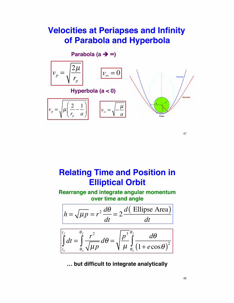
Hyperbola (a < 0)
Velocities at Periapses and Infinity of Parabola and Hyperbola
47
vp =2µrp
Parabola (a "" ")
v! = 0
v! = " µa
Relating Time and Position in Elliptical Orbit
Rearrange and integrate angular momentum over time and angle
h = µp = r2 d!dt
= 2 d Ellipse Area( )dt
48
dtto
t f
! = r2
µpd"
"o
" f
! = p3
µd"
1+ ecos"( )2"o
" f
!
… but difficult to integrate analytically
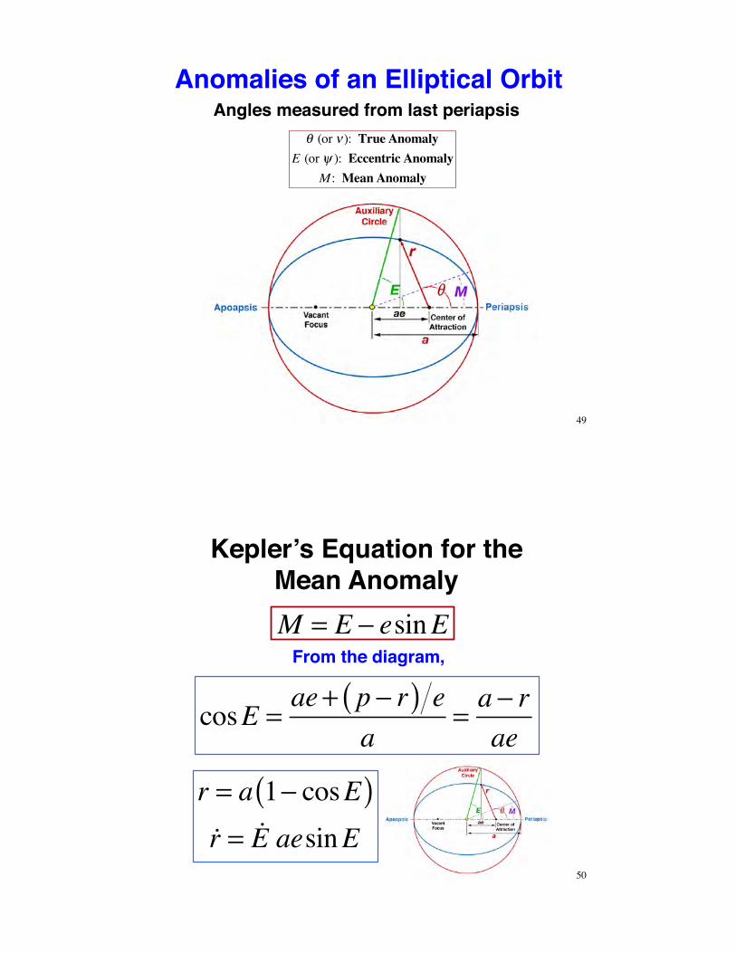
Anomalies of an Elliptical OrbitAngles measured from last periapsis
49
! (or " ): True AnomalyE (or # ): Eccentric Anomaly
M : Mean Anomaly
50
Kepler’s Equation for the Mean AnomalyM = E ! esinE
cosE =ae+ p ! r( ) e
a= a ! r
ae
r = a 1! cosE( )!r = !E aesinE
From the diagram,
51
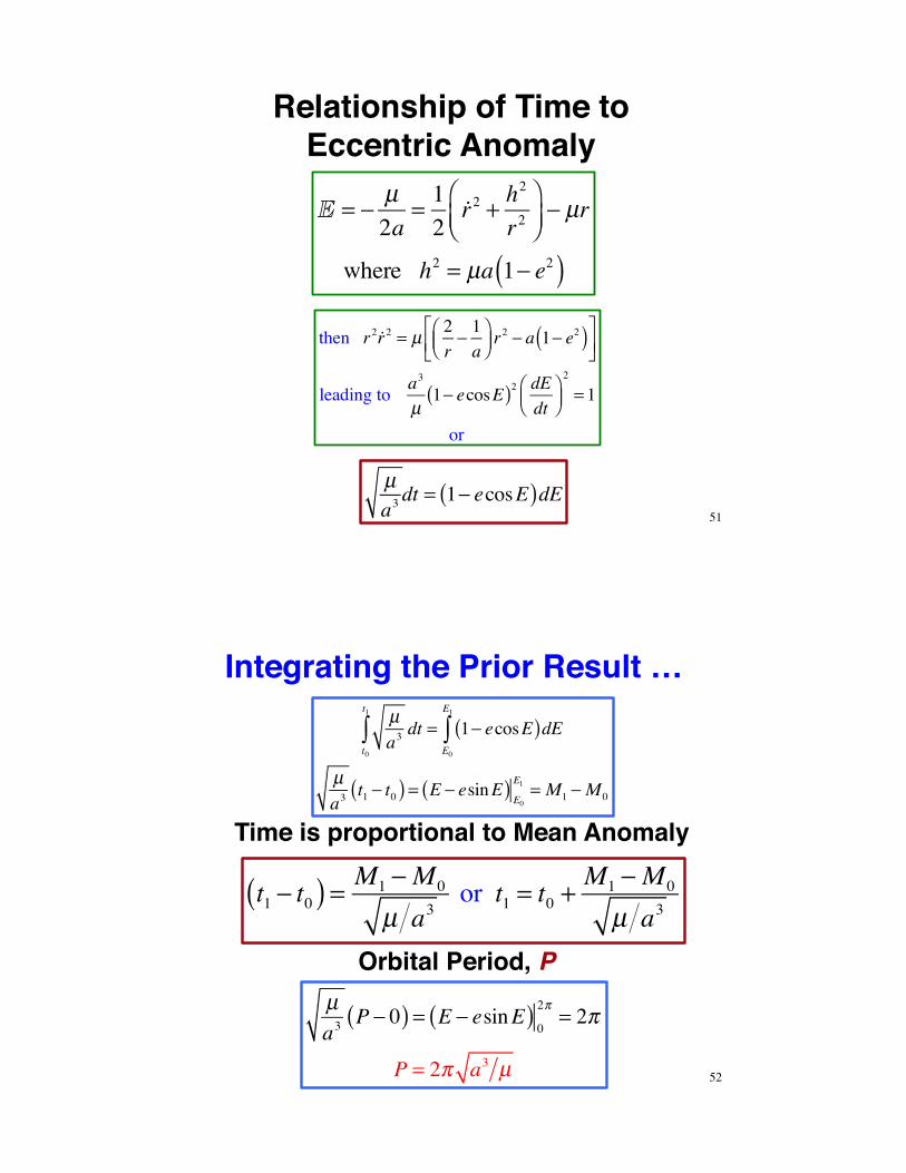
Relationship of Time to Eccentric Anomaly
E = ! µ2a
= 12!r2 + h
2
r2
"#$
%&'! µr
where h2 = µa 1! e2( )
then r2 !r2 = µ 2r! 1a
"#$
%&' r
2 ! a 1! e2( )()*
+,-
leading to a3
µ1! ecosE( )2 dE
dt"#$
%&'
2
= 1
or
µa3dt = 1! ecosE( )dE
52
Integrating the Prior Result …µa3dt
t0
t1
! = 1" ecosE( )dEE0
E1
!µa3
t1 " t0( ) = E " esinE( ) E0E1 = M1 "M 0
t1 ! t0( ) = M1 !M 0
µ a3 or t1 = t0 +
M1 !M 0
µ a3
µa3
P ! 0( ) = E ! esinE( ) 02"
= 2"
P = 2" a3 µ
Orbital Period, P
Time is proportional to Mean Anomaly

Orbital Period
Orbital period is related to the total energy
P = 2! a3
µ= ! "µ2
2E 3 where E < 0 for an ellipse
53
Mean Motion, n, is the inverse of the Period
P = 2! a3
µ!
2!n
where n is the Mean Motion
Position and Velocity in Orbit at Time, tMean Anomaly, given time from perigee passage, tp
54
M t( ) = µa3
t ! t p( )Eccentric Anomaly, E(t), given Mean Anomaly, M(t)
E t( )! esinE t( ) = M t( )
Eo t( ) = M t( ) + esinM t( )Iterate until !Mi < Tolerance
!Mi = M t( )" Ei t( )" esinEi t( )#$ %&!Ei+1 = !Mi 1" ecosEi t( )#$ %&
Ei+1 t( ) = Ei t( ) + !Ei+1
Newton’s method of successive approximation, using M(t) as starting guess for E(t)

Position and Velocity in Orbit at Time, tCalculate True Anomaly, given Eccentric Anomaly
55
! t( ) = 2 tan"1 1+ e1" e
tan E t( )2
#
$%
&
'(
Compute magnitude of radius
r t( ) = a 1! e2( )1+ ecos" t( )
Position and Velocity in Orbit at Time, t
56
Radius vector, in the orbital plane
r t( ) =x t( )y t( )
!
"##
$
%&&=
r t( )cos' t( )r t( )sin' t( )
!
"##
$
%&&
Velocity vector, in the orbital plane
v t( ) =vx t( )vy t( )
!
"
##
$
%
&&= µ
p'sin( t( )e+ cos( t( )
!
"##
$
%&&
see Weisel, Spaceflight Dynamics, 1997, pp. 64-66

!!eexxtt TTiimmee::""llaanneettaarryy DDeeffeennssee
57
##uupppplleemmeennttaall MMaa$$rriiaall
58

First Point of Aries!(Ecliptic Intercept at Right)"
59
Dimension of energy?"
Dimension of linear momentum?"
Dimension of angular momentum?"
Scalar (1 x 1)"
Vector (3 x 1)"
Vector (3 x 1)"60

Sub-Orbital (Sounding) Rockets 1945 - Present
NASA Wallops Island Control Center
CanadianBlack Brant XII
LTVScout
61
MATLAB Code for Flat-Earth Trajectories
Script for Analytic Solution
g = 9.8; t = 0:0.1:40; vx0 = 10; vz0 = 100; x0 = 0; z0 = 0; vx1 = vx0; vz1 = vz0 – g*t; x1 = x0 + vx0*t; z1 = z0 + vz0*t - 0.5*g*t.* t;
Script for Numerical Solution
tspan = 40; % Time span, sxo = [10;100;0;0]; % Init. Cond.[t1,x1] = ode45('FlatEarth',tspan,xo);
Function for Numerical Solution
function xdot = FlatEarth(t,x) % x(1) = vx% x(2) = vz% x(3) = x% x(4) = z g = 9.8; xdot(1) = 0; xdot(2) = -g; xdot(3) = x(1); xdot(4) = x(2); xdot = xdot';end 62

Trajectories Calculated with Flat-Earth Model
!! Constant gravity, g, is the only force in the model, i.e., no aerodynamic or thrust force
!! Can neglect motions in the y direction
vx t( ) = vx0
!vz t( ) = !g z positive up( )!x t( ) = vx t( )!z t( ) = vz t( )
vx 0( ) = vx0vz 0( ) = vz0x 0( ) = x0z 0( ) = z0
Dynamic Equations
Initial Conditions
vx T( ) = vx0vz T( ) = vz0 ! gdt
0
T
" = vz0 ! gT
x T( ) = x0 + vx0T
z T( ) = z0 + vz0T ! gt dt0
T
" = z0 + vz0T ! gT 2 2
Analytic (Closed-Form) Solution
63
Trajectories Calculated with Flat-Earth Model
vx 0( ) = 10m / svz 0( ) = 100,150, 200m / sx 0( ) = 0z 0( ) = 0
64

MATLAB Code for Spherical-Earth Trajectories
Script for Numerical Solution R = 6378; % Earth Surface Radius, km tspan = 6000; % seconds options = odeset('MaxStep', 10) xo = [7.5;0;0;R]; [t1,x1] = ode15s('RoundEarth',tspan,xo,options); for i = 1:length(t1) v1(i) = sqrt(x1(i,1)*x1(i,1) + x1(i,2)*x1(i,2)); r1(i) = sqrt(x1(i,3)*x1(i,3) + x1(i,4)*x1(i,4)); end
function xdot = RoundEarth(t,x)% x(1) = vx% x(2) = vy% x(3) = x% x(4) = y mu = 3.98*10^5; % km^2/s^2 r = sqrt(x(3)^2 + x(4)^2); xdot(1) = -mu * x(3) / r^3; xdot(2) = -mu * x(4) / r^3; xdot(3) = x(1); xdot(4) = x(2); xdot = xdot';end
Function for Numerical Solution
65
x2
a2 +y2
b2 = 1
a : Semi - major axis, m or kmb : Semi - minor axis, m or km
x !( ) = a cos !( )y !( ) = b sin !( )
! : Angle from x - axis (origin at center) rad
Equations that Describe Ellipses
a ob
yx
66
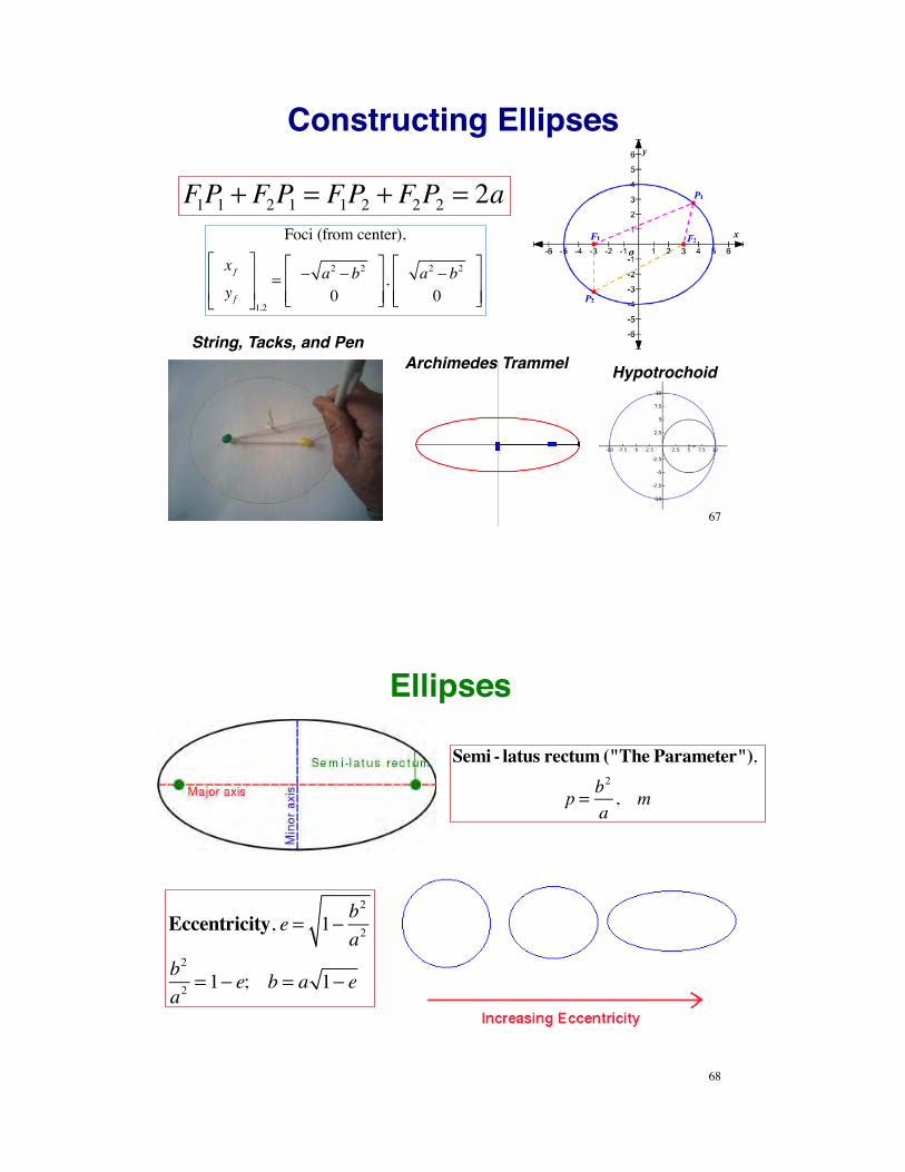
Constructing Ellipses
F1P1 + F2P1 = F1P2 + F2P2 = 2a
String, Tacks, and Pen
HypotrochoidArchimedes Trammel
Foci (from center),
x fy f
!
"##
$
%&&
1,2
= ' a2 ' b2
0
!
"##
$
%&&, a2 ' b2
0
!
"##
$
%&&
67
Ellipses
Eccentricity, e = 1! b2
a2
b2
a2= 1! e; b = a 1! e
Semi - latus rectum ("The Parameter"),
p = b2
a, m
68

How Do We Know that Gravitational Force is Conservative?
Because the force is the derivative (with respect to r) of a scalar function of r called
the potential, V(r):
V r( ) = !m µr+Vo = !m µ
rTr( )1 2+Vo
!V r( )!r
=!V !x!V !y!V !z
"
#
$$$
%
&
'''= m µ
r3
xyz
"
#
$$$
%
&
'''= (Fg
This derivative is also called the gradient of V with respect to r 69
Conservation of EnergyEnergy is conserved in an elastic collision, i.e. no
losses due to friction, air drag, etc.“Newton’s Cradle” illustrates interchange of
potential and kinetic energy in a gravitational field
70

Examples of Circular Orbit Periods for Earth and Moon
Period, minAltitude above
Surface, km Earth Moon0 84.5 108.5
100 86.5 1181000 105.1 214.610000 347.7 1905
71
Typical Satellite Orbits
Sun-Synchronous
Orbit
GPS Constellation
26,600 km
72
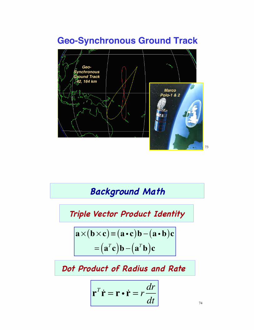
Geo-Synchronous Ground Track
Geo-Synchronous Ground Track
42, 164 km
Marco Polo-1 & 2
73
Background Math"
a ! b ! c( ) " a i c( )b # a ib( )c= aTc( )b # aTb( )c
Triple Vector Product Identity"
rT !r = r i !r = r dr
dt
Dot Product of Radius and Rate "
74


