

Learning From DataLecture 9
Logistic Regression and Gradient Descent
Logistic RegressionGradient Descent
M. Magdon-IsmailCSCI 4100/6100
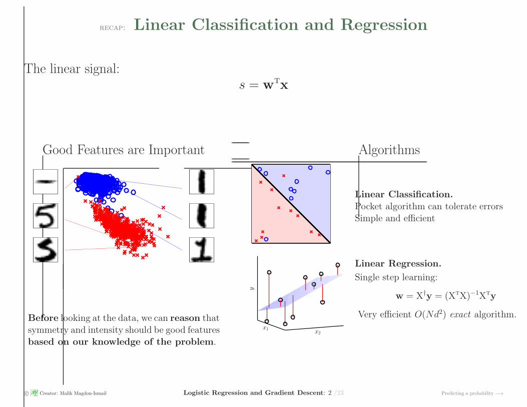
recap: Linear Classification and Regression
The linear signal:s = wtx
Good Features are Important Algorithms
Before looking at the data, we can reason thatsymmetry and intensity should be good featuresbased on our knowledge of the problem.
Linear Classification.
Pocket algorithm can tolerate errorsSimple and efficient
x1x2
y
Linear Regression.
Single step learning:
w = X†y = (XtX)−1Xty
Very efficient O(Nd2) exact algorithm.
c© AML Creator: Malik Magdon-Ismail Logistic Regression and Gradient Descent: 2 /23 Predicting a probability −→

Predicting a Probability
Will someone have a heart attack over the next year?
age 62 years
gender male
blood sugar 120 mg/dL40,000
HDL 50
LDL 120
Mass 190 lbs
Height 5′ 10′′
. . . . . .
Classification: Yes/No
Logistic Regression: Likelihood of heart attack logistic regression ≡ y ∈ [0, 1]
h(x) = θ
(d∑
i=0
wixi
)
= θ(wtx)
c© AML Creator: Malik Magdon-Ismail Logistic Regression and Gradient Descent: 3 /23 What is θ? −→

Predicting a Probability
Will someone have a heart attack over the next year?
age 62 years
gender male
blood sugar 120 mg/dL40,000
HDL 50
LDL 120
Mass 190 lbs
Height 5′ 10′′
. . . . . .
Classification: Yes/No
Logistic Regression: Likelihood of heart attack logistic regression ≡ y ∈ [0, 1]
h(x) = θ
(d∑
i=0
wixi
)
= θ(wtx)θ(s)
1
0 s
θ(s) =es
1 + es=
1
1 + e−s
.
θ(−s) =e−s
1 + e−s
=1
1 + es= 1− θ(s).
c© AML Creator: Malik Magdon-Ismail Logistic Regression and Gradient Descent: 4 /23 Data is binary ±1 −→
The Data is Still Binary, ±1
D = (x1, y1 = ±1), · · · , (xN , yN = ±1)
xn ← a person’s health information
yn = ±1 ← did they have a heart attack or not
We cannot measure a probability.
We can only see the occurence of an event and try to infer a probability.
c© AML Creator: Malik Magdon-Ismail Logistic Regression and Gradient Descent: 5 /23 f is noisy −→
The Target Function is Inherently Noisy
f(x) = P[y = +1 | x].
The data is generated from a noisy target function:
P (y | x) =
f(x) for y = +1;
1− f(x) for y = −1.
c© AML Creator: Malik Magdon-Ismail Logistic Regression and Gradient Descent: 6 /23 When is h good? −→

What Makes an h Good?
‘fitting’ the data means finding a good h
h is good if:
h(xn) ≈ 1 whenever yn = +1;
h(xn) ≈ 0 whenever yn = −1.
A simple error measure that captures this:
Ein(h) =1
N
N∑
n=1
(h(xn)−
12(1 + yn)
)2.
Not very convenient (hard to minimize).
c© AML Creator: Malik Magdon-Ismail Logistic Regression and Gradient Descent: 7 /23 Cross entropy error −→

The Cross Entropy Error Measure
Ein(w) =1
N
N∑
n=1
ln(1 + e−yn·wtx)
It looks complicated and ugly (ln, e(·), . . .),
But,– it is based on an intuitive probabilistic interpretation of h.
– it is very convenient and mathematically friendly (‘easy’ to minimize).
Verify: yn = +1 encourages wtxn ≫ 0, so θ(wtxn) ≈ 1; yn = −1 encourages wtxn ≪ 0, so θ(wtxn) ≈ 0;
c© AML Creator: Malik Magdon-Ismail Logistic Regression and Gradient Descent: 8 /23 Probabilistic interpretation −→

The Probabilistic Interpretation
Suppose that h(x) = θ(wtx) closely captures P[+1|x]:
P (y | x) =
θ(wtx) for y = +1;
1− θ(wtx) for y = −1.
c© AML Creator: Malik Magdon-Ismail Logistic Regression and Gradient Descent: 9 /23 1− θ(s) = θ(−s) −→

The Probabilistic Interpretation
So, if h(x) = θ(wtx) closely captures P[+1|x]:
P (y | x) =
θ(wtx) for y = +1;
θ(−wtx) for y = −1.
c© AML Creator: Malik Magdon-Ismail Logistic Regression and Gradient Descent: 10 /23 Simplify to one equation −→

The Probabilistic Interpretation
So, if h(x) = θ(wtx) closely captures P[+1|x]:
P (y | x) =
θ(wtx) for y = +1;
θ(−wtx) for y = −1.
. . . or, more compactly,P (y | x) = θ(y ·wtx)
c© AML Creator: Malik Magdon-Ismail Logistic Regression and Gradient Descent: 11 /23 The likelihood −→
The Likelihood
P (y | x) = θ(y ·wtx)
Recall: (x1, y1), . . . , (xN , yN) are independently generated
Likelihood:The probability of getting the y1, . . . , yN in D from the corresponding x1, . . . ,xN :
P (y1, . . . , yN | x1, . . . ,xn) =N∏
n=1
P (yn | xn).
The likelihood measures the probability that the data were generated if f were h.
c© AML Creator: Malik Magdon-Ismail Logistic Regression and Gradient Descent: 12 /23 Maximize the likelihood −→

Maximizing The Likelihood (why?)
max∏N
n=1P (yn | xn)
⇔ max ln(∏N
n=1P (yn | xn))
≡ max∑N
n=1 lnP (yn | xn)
⇔ min − 1N
∑Nn=1 lnP (yn | xn)
≡ min 1N
∑Nn=1 ln
1P (yn|xn)
≡ min 1N
∑Nn=1 ln
1θ(yn·wtxn)
← we specialize to our “model” here
≡ min 1N
∑Nn=1 ln(1 + e−yn·w
txn)
Ein(w) =1
N
N∑
n=1
ln(1 + e−yn·wtxn)
c© AML Creator: Malik Magdon-Ismail Logistic Regression and Gradient Descent: 13 /23 How to minimize Ein(w) −→

How To Minimize Ein(w)
Classification – PLA/Pocket (iterative)
Regression – pseudoinverse (analytic), from solving ∇wEin(w) = 0.
Logistic Regression – analytic won’t work.
Numerically/iteratively set ∇wEin(w)→ 0.
c© AML Creator: Malik Magdon-Ismail Logistic Regression and Gradient Descent: 14 /23 Hill analogy −→

Finding The Best Weights - Hill Descent
Ball on a complicated hilly terrain
— rolls down to a local valley
↑this is called a local minimum
Questions:
How to get to the bottom of the deepest valey?
How to do this when we don’t have gravity?
c© AML Creator: Malik Magdon-Ismail Logistic Regression and Gradient Descent: 15 /23 Our Ein is convex −→

Our Ein Has Only One Valley
Weights, w
In-sam
pleError,E
in
. . . because Ein(w) is a convex function of w. (So, who care’s if it looks ugly!)
c© AML Creator: Malik Magdon-Ismail Logistic Regression and Gradient Descent: 16 /23 How to roll down? −→

How to “Roll Down”?
Assume you are at weights w(t) and you take a step of size η in the direction v̂.
w(t + 1) = w(t) + ηv̂
We get to pick v̂ ← what’s the best direction to take the step?
Pick v̂ to make Ein(w(t + 1)) as small as possible.
c© AML Creator: Malik Magdon-Ismail Logistic Regression and Gradient Descent: 17 /23 The gradient −→

The Gradient is the Fastest Way to Roll Down
Approximating the change in Ein
∆Ein = Ein(w(t+ 1))− Ein(w(t))
= Ein(w(t) + ηv̂)− Ein(w(t))
= η∇Ein(w(t))tv̂
︸ ︷︷ ︸
minimized at v̂ = − ∇Ein(w(t))|| ∇Ein(w(t)) ||
+O(η2) (Taylor’s Approximation)
>≈ −η||∇Ein(w(t)) || ←attained at v̂ = − ∇Ein(w(t))
|| ∇Ein(w(t)) ||
The best (steepest) direction to move is the negative gradient:
v̂ = −
∇Ein(w(t))
|| ∇Ein(w(t)) ||
c© AML Creator: Malik Magdon-Ismail Logistic Regression and Gradient Descent: 18 /23 Iterate the gradient −→

“Rolling Down” ≡ Iterating the Negative Gradient
w(0)↓ ← negative gradient
w(1)↓ ← negative gradient
w(2)↓ ← negative gradient
w(3)↓ ← negative gradient
... η = 0.5; 15 steps
c© AML Creator: Malik Magdon-Ismail Logistic Regression and Gradient Descent: 19 /23 What step size? −→

The ‘Goldilocks’ Step Size
η too small η too large variable ηt – just right
Weights, w
In-sam
pleError,E
in
Weights, w
In-sam
pleError,E
in
Weights, w
In-sam
pleError,E
in
large η
small η
η = 0.1; 75 steps η = 2; 10 steps variable ηt; 10 steps
c© AML Creator: Malik Magdon-Ismail Logistic Regression and Gradient Descent: 20 /23 Fixed learning rate gradient descent −→

Fixed Learning Rate Gradient Descent
ηt = η · || ∇Ein(w(t)) ||
|| ∇Ein(w(t)) || → 0 when closer to the minimum.
v̂ = −ηt ·∇Ein(w(t))
||∇Ein(w(t)) ||
= −η · ||∇Ein(w(t)) || ·∇Ein(w(t))
||∇Ein(w(t)) ||
v̂ = −η · ∇Ein(w(t))
1: Initialize at step t = 0 to w(0).2: for t = 0, 1, 2, . . . do
3: Compute the gradient
gt = ∇Ein(w(t)). ←− (Ex. 3.7 in LFD)
4: Move in the direction vt = −gt.5: Update the weights:
w(t+ 1) = w(t) + ηvt.
6: Iterate ‘until it is time to stop’.7: end for
8: Return the final weights.
Gradient descent can minimize any smooth function, for example
Ein(w) =1
N
N∑
n=1
ln(1 + e−yn·wtx) ← logistic regression
c© AML Creator: Malik Magdon-Ismail Logistic Regression and Gradient Descent: 21 /23 Stochastic gradient descent −→

Stochastic Gradient Descent (SGD)
A variation of GD that considers only the error on one data point.
Ein(w) =1
N
N∑
n=1
ln(1 + e−yn·wtx) =
1
N
N∑
n=1
e(w,xn, yn)
• Pick a random data point (x∗, y∗)
• Run an iteration of GD on e(w,x∗, y∗)
w(t + 1)← w(t)− η∇we(w,x∗, y∗)
1. The ‘average’ move is the same as GD;
2. Computation: fraction 1N
cheaper per step;
3. Stochastic: helps escape local minima;
4. Simple;
5. Similar to PLA.
Logistic Regression:
w(t + 1)← w(t) + y∗x∗
(η
1 + ey∗wtx∗
)
(Recall PLA: w(t+ 1)← w(t) + y∗x∗)
c© AML Creator: Malik Magdon-Ismail Logistic Regression and Gradient Descent: 22 /23 GD versus SGD, a picture −→

Stochastic Gradient Descent
GD SGD
η = 610 stepsN = 10
η = 230 steps
c© AML Creator: Malik Magdon-Ismail Logistic Regression and Gradient Descent: 23 /23


