

Learning in ArtificialSensorimotor Systems
Daniel D. Lee
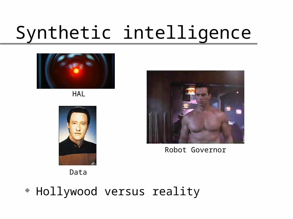
Synthetic intelligence
Hollywood versus reality
Data
HAL
Robot Governor
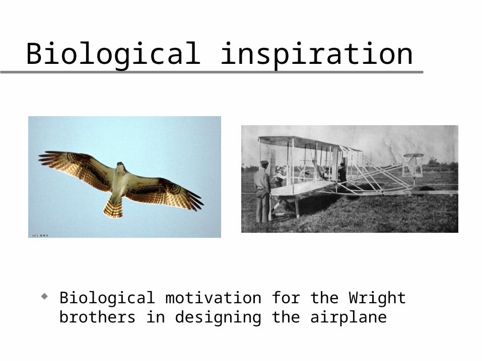
Biological inspiration
Biological motivation for the Wright brothers in designing the airplane

Robot dogs
Platforms for testing sensorimotor machine learning algorithms
Custom built version Sony Aibos
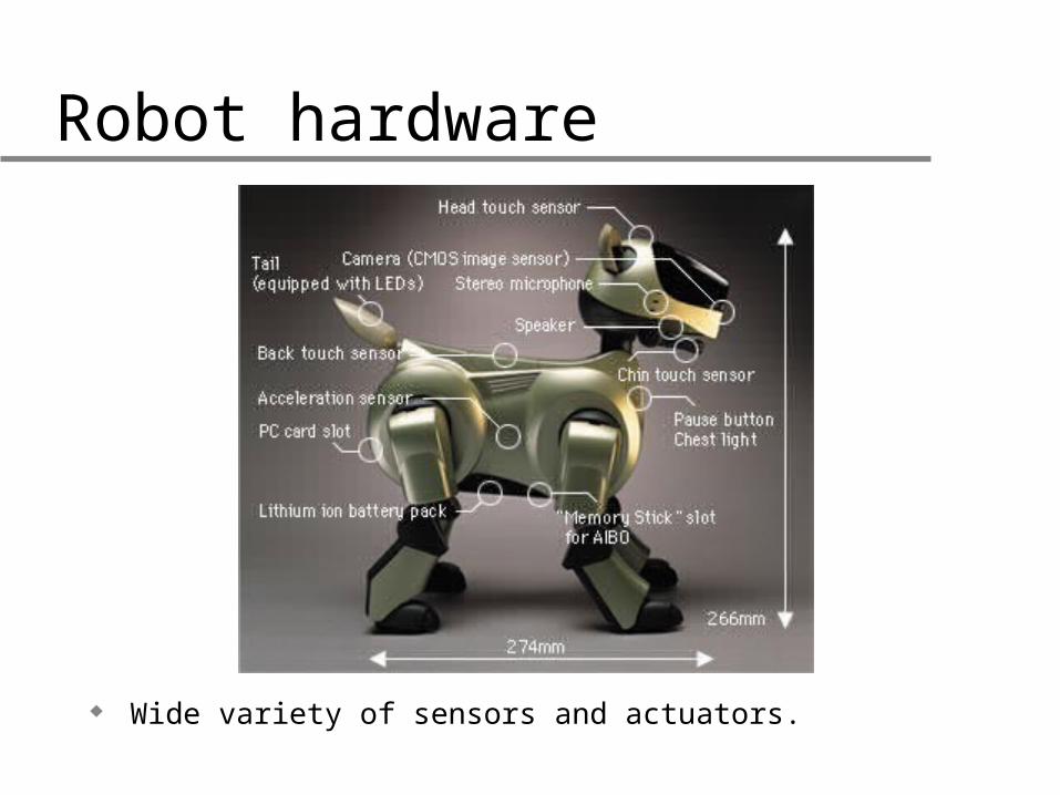
Robot hardware
Wide variety of sensors and actuators.

Robocup
Grand challenge for robotics community
Legged league Humanoid league
Middle size leagueSmall size league
Simulation league

Legged league
Recently implemented larger field and wireless communications among robots.
Each team consists of 4 Sony Aibo robot dogs (one is a designated goalie), with WiFi communications.
Field is 3 by 5 meters, with orange ball and specially colored markers.
Game played in two halves, each 10 minutes in duration. Teams change uniform color at half-time.
Human referees govern kick-off formations, holding, penalty area violations, goalie charging, etc.
Penalty kick shootout in case of ties in elimination round.

Upennalizers in action
GOOAAALLL! 2nd place in 2003.

Robot software architecture
Cognition(Plan)
Action(Actuators)
Perception(Sensors)
Sense-Plan-Act cycle.

Perception
View from Penn’somnidirectional camera

Robot vision
Color segmentation: estimate P(Y,Cb,Cr | ORANGE) from training images
Region formation: run length encoding, union find algorithm
Distance calibration: bounding box size and elevation angle
Camera geometry: transformation from camera to body centered coordinates
Tracking objects in structured environment at 25 fps
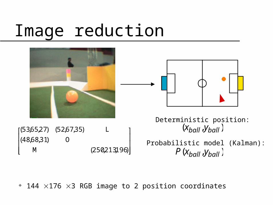
Image reduction
144 176 3 RGB image to 2 position coordinates
€
(53,65,27) (52,67,35) L
(48,68,31) O
M (250,213,196)
⎡
⎣
⎢ ⎢ ⎢
⎤
⎦
⎥ ⎥ ⎥
€
(xball , yball )
€
P(xball , yball )
Deterministic position:
Probabilistic model (Kalman):

Image manifolds
Variation in pose and illumination give rise to low dimensional manifold structure
Pixel vector
€
0.0
0.5
0.7
1.0
M
0.8
0.2
0.0
⎡
⎣
⎢ ⎢ ⎢ ⎢ ⎢ ⎢ ⎢ ⎢ ⎢ ⎢
⎤
⎦
⎥ ⎥ ⎥ ⎥ ⎥ ⎥ ⎥ ⎥ ⎥ ⎥

Learning nonlinear manifolds
Many recent algorithms for nonlinear manifolds.
Kernel PCA, Isomap, LLE, Laplacian Eigenmaps, etc.

Locally linear embedding
LLE solves two quadratic optimizations using eigenvector methods (Roweis & Saul).
€
E(W ) =r X i − Wij
r X j
j∑
2
i∑
€
Φ(Y ) =r Y i − Wij
r Y j
j∑
2
i∑

Translational invariance
Application of LLE for translational invariance.

Action
M. Raibert’s hoppingrobot (1983)

Inverse kinematics
QuickTime™ and aTIFF (Uncompressed) decompressor
are needed to see this picture.
Degenerate solutions with many articulators.
€
H = R(θ1)oT (l1)oR(θ2 )oT (l2 )oR(θ3)oT (l3)
€
θ1
€
θ2
€
θ3
€
l1
€
l2
€
l3

Gaits
4-legged animal gaits

Walking
Parameters tuned by optimization techniques
Inverse kinematics to calculate joint angles in shoulder and knee

Behavior
SRI’s Shakey (1970)

Probabilistic localization
∑==
iii yxPP
PyxP
yxP
)|,()(
)()|,(
),,(
θθ
θθ
θ
Particle filter Kalman filter
Kalman and particle filters used to represent pose
x,y

Finite state machine
Event driven state machine.
Search forball
Goto ballposition
Kick ball
Seeball
Closeto ball
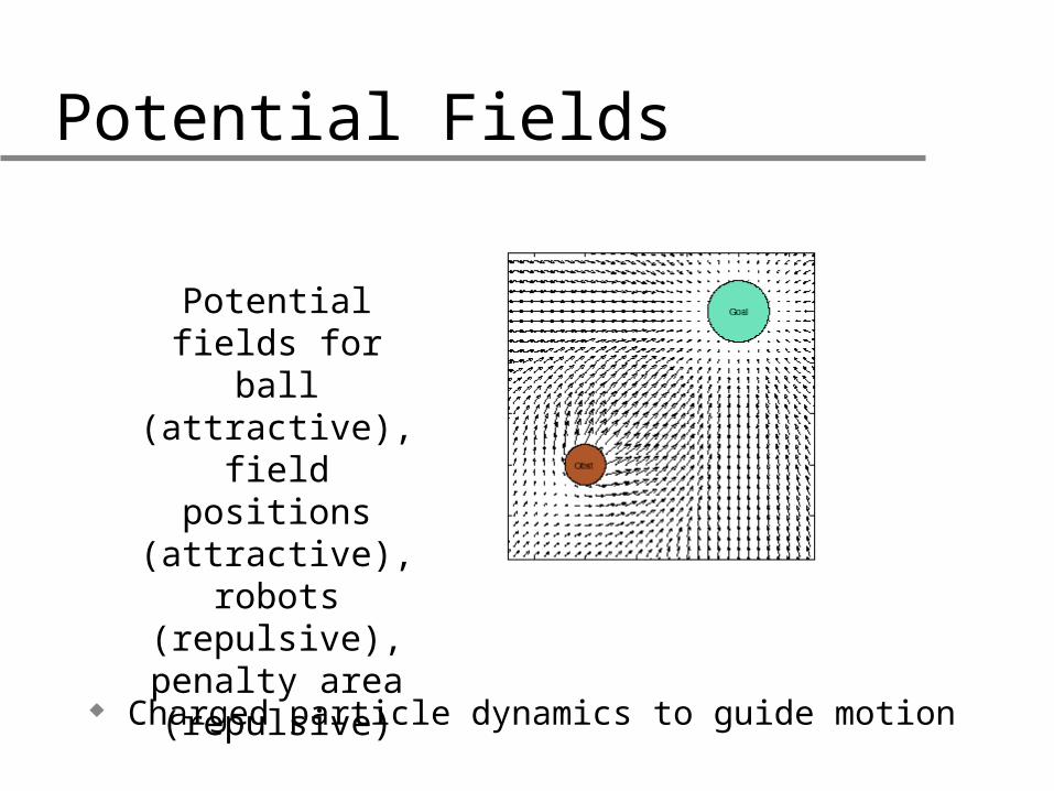
Potential Fields
Charged particle dynamics to guide motion
Potential fields forball (attractive), field positions
(attractive), robots (repulsive), penalty
area (repulsive)

Learning behaviors
Reinforcement learning for control parameters
AttackSupport
Defend
Goalie
Potential field parametersState selectionRole switchingAdaptive strategies

Reactive behaviors
“Behavior-based” robotics maps sensors to actuators without complex reasoning

Stimulus-response mapping
Stimulus space Response space
Construct low dimensional representations for mapping stimulus to response
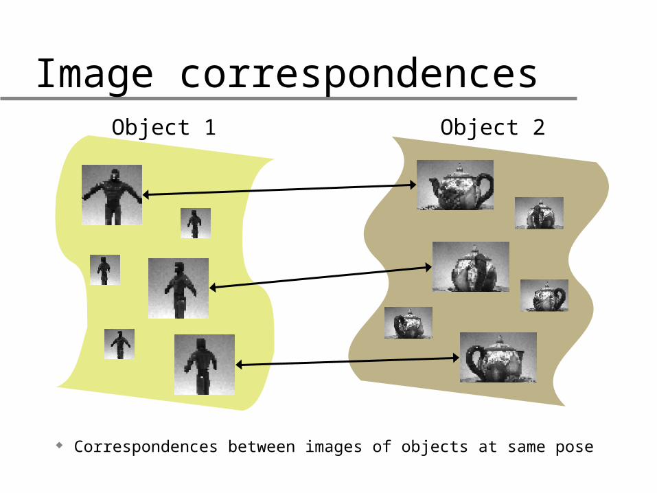
Image correspondencesObject 1 Object 2
Correspondences between images of objects at same pose
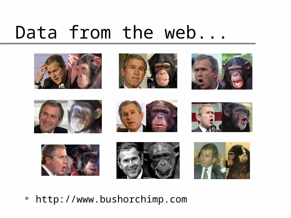
Data from the web...
http://www.bushorchimp.com

Learning from examplesGiven Data (X1,X2):
n labeledcorrespondences
N1 examplesof object 1
(D1 dimensions)
N2 examplesof object 2
(D2 dimensions)
Matrix formulation (n << N1, N2 )
?
?D1N1D1n
D2n
D2N
2
X1
X2

Supervised learning
Problem overfitting with small amount of labeled data
Fill in the blanks:
(D1 +D2 ) n labeled dataD1 D2 parameters
?
?D1N1D1n
D2n
D2N
2
TrainingData
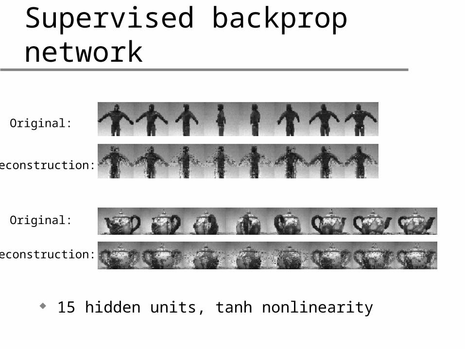
Supervised backprop network
Original:
Reconstruction:
Original:
Reconstruction:
15 hidden units, tanh nonlinearity

Missing data
Treat as missing data problem using EM algorithm
EM algorithm:
Iteratively fills in missing data statistics, reestimatesparameters for PCA, factor analysis
?
?D1N1D1n
D2n
D2N
2
D1+D2
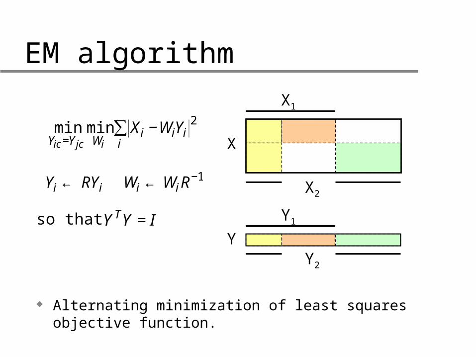
EM algorithm
€
minYic=Yjc
minWi
Xi −WiYii
∑ 2
€
Yi ← RYi
Alternating minimization of least squares objective function.
€
Y TY = I Y1
Y2
X
Yso that
€
Wi ←WiR−1
X1
X2

PCA with correspondences
15 dimensional subspace, 200 images of each object, 10 in correspondence
Original:
Original:

Factor analysis
Original:
Original:
15 dimensional subspace with diagonal noise covariance

Common embedding space
Two input spaces Common low dimensional space

LLE with correspondences
Quadratic optimization with constraints is solved with spectral decomposition
Correspondences:
€
E(W1) =r X i
1 − Wij1 r X j
1
j∑
2
i∑
€
E(W 2 ) =r X i
2 − Wij2 r X j
2
j∑
2
i∑
€
Φ(Y1,Y 2 ) =r Y i
1 − Wij1 r Y j
1
j∑
2
i∑
€
+r Y i
2 − Wij2 r Y j
2
j∑
2
i∑
€
i∈Sc :r Y i
1 =r Y i
2
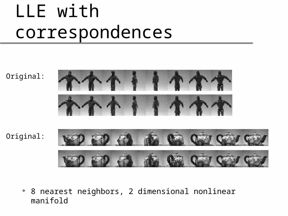
LLE with correspondences
Original:
Original:
8 nearest neighbors, 2 dimensional nonlinear manifold

Quantitative comparison
Incorporating manifold structure improves reconstruction error.
Correspondence fraction
Nor
mal
ized
err
or

Summary
Adaptation and learning in biological systems for sensorimotor processing.
Many sensory and motor activations are described by an underlying manifold structure.
Development of learning algorithms that can incorporate this low dimensional manifold structure.
Still much room for improvement…


