
Stanford 2010 Trevor Hastie, Stanford Statistics 1
Learning with SparsityConstraints
Trevor Hastie
Stanford University
recent joint work with Rahul Mazumder, Jerome Friedman and Rob Tibshirani
earlier work with Brad Efron, Ji Zhu, Saharon Rosset, Hui Zou and Mee-Young Park
Stanford 2010 Trevor Hastie, Stanford Statistics 2
Linear Models in Data Mining
As datasets grow wide—i.e. many more predictors than
samples—linear models have regained popularity.
Document classification: bag-of-words can leads to p = 20K
features and N = 5K document samples.
Image deblurring, classification: p = 65K pixels are features,
N = 100 samples.
Genomics, microarray studies: p = 40K genes are measured
for each of N = 100 subjects.
Genome-wide association studies: p = 500K SNPs measured
for N = 2000 case-control subjects.
In all of these we use linear models — e.g. linear regression, logistic
regression, Cox model. Since p≫ N , we have to regularize.
Stanford 2010 Trevor Hastie, Stanford Statistics 3
Forms of Regularization
We cannot fit linear models with p > N without some constraints.
Common approaches are
Forward stepwise adds variables one at a time and stops when
overfitting is detected. This is a greedy algorithm, since the
model with say 5 variables is not necessarily the best model of
size 5.
Best-subset regression finds the subset of each size k that fits the
model the best. Only feasible for small p around 35.
Ridge regression fits the model subject to constraint∑p
j=1 β2j ≤ t. Shrinks coefficients toward zero, and hence
controls variance. Allows linear models with arbitrary size p to
be fit, although coefficients always in row-space of X .
Stanford 2010 Trevor Hastie, Stanford Statistics 4
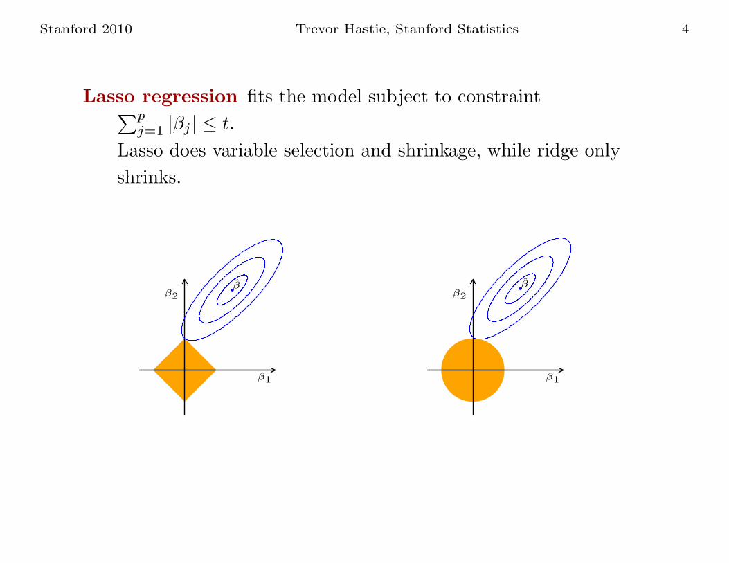
Lasso regression fits the model subject to constraint∑p
j=1 |βj | ≤ t.
Lasso does variable selection and shrinkage, while ridge only
shrinks.
β2
β1
ββ2
β1
β
Stanford 2010 Trevor Hastie, Stanford Statistics 5
Brief History of ℓ1 Regularization
minβ
N∑
i=1
(yi − β0 −
p∑
j=1
xijβj)2 subject to
p∑
j=1
|βj | ≤ t
• Wavelet Soft Thresholding (Donoho and Johnstone 1994) in
orthonormal setting.
• Tibshirani introduces Lasso for regression in 1995.
• Same idea used in Basis Pursuit (Chen, Donoho and Saunders
1996).
• Extended to many linear-model settings e.g. Survival models
(Tibshirani, 1997), logistic regression, and so on.
• Gives rise to a new field Compressed Sensing (Donoho 2004,
Candes and Tao 2005)—near exact recovery of sparse signals in
very high dimensions. In many cases ℓ1 a good surrogate for ℓ0.
Stanford 2010 Trevor Hastie, Stanford Statistics 6
0.0 0.2 0.4 0.6 0.8 1.0
−50
00
500
52
110
84
69
0 2 3 4 5 7 8 10
||β(λ)||1/||β(0)||1
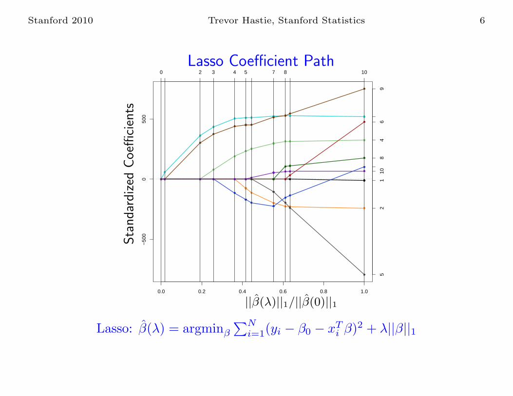
Lasso Coefficient Path
Sta
ndard
ized
Coeffi
cie
nts
Lasso: β(λ) = argminβ
∑Ni=1(yi − β0 − xT
i β)2 + λ||β||1
Stanford 2010 Trevor Hastie, Stanford Statistics 7
History of Path Algorithms
Efficient path algorithms for β(λ) allow for easy and exact
cross-validation and model selection.
• In 2001 the LARS algorithm (Efron et al) provides a way to
compute the entire lasso coefficient path efficiently at the cost
of a full least-squares fit.
• 2001 – present: path algorithms pop up for a wide variety of
related problems: Grouped lasso (Yuan & Lin 2006),
support-vector machine (Hastie, Rosset, Tibshirani & Zhu
2004), elastic net (Zou & Hastie 2004), quantile regression (Li
& Zhu, 2007), logistic regression and glms (Park & Hastie,
2007), Dantzig selector (James & Radchenko 2008), ...
• Many of these do not enjoy the piecewise-linearity of LARS,
and seize up on very large problems.
Stanford 2010 Trevor Hastie, Stanford Statistics 8
Coordinate Descent
• Solve the lasso problem by coordinate descent: optimize each
parameter separately, holding all the others fixed. Updates are
trivial. Cycle around till coefficients stabilize.
• Do this on a grid of λ values, from λmax down to λmin
(uniform on log scale), using warms starts.
• Can do this with a variety of loss functions and additive
penalties.
Coordinate descent achieves dramatic speedups over all
competitors, by factors of 10, 100 and more.
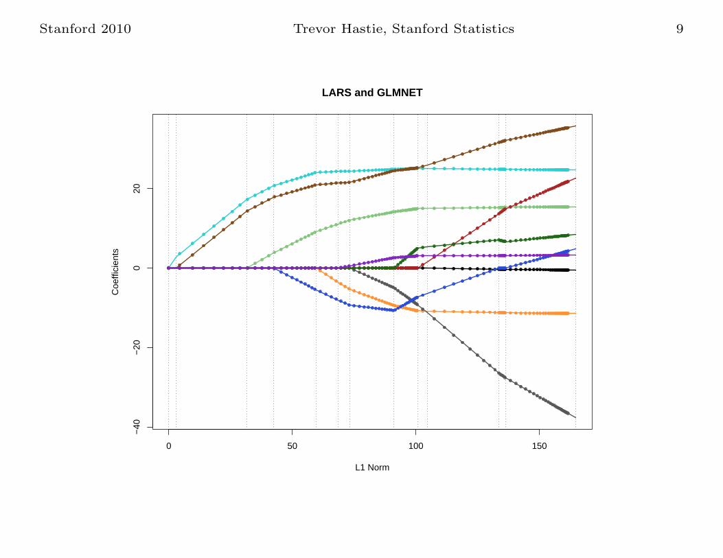
Stanford 2010 Trevor Hastie, Stanford Statistics 9
0 50 100 150
−40
−20
020
L1 Norm
Coe
ffici
ents
LARS and GLMNET
Stanford 2010 Trevor Hastie, Stanford Statistics 10
Speed Trials on Large Datasets
Competitors:
glmnet Fortran based R package using coordinate descent. Covers
GLMs and Cox model.
l1logreg Lasso-logistic regression package by Koh, Kim and Boyd,
using state-of-art interior point methods for convex
optimization.
BBR/BMR Bayesian binomial/multinomial regression package by
Genkin, Lewis and Madigan. Also uses coordinate descent to
compute posterior mode with Laplace prior—the lasso fit.
Stanford 2010 Trevor Hastie, Stanford Statistics 11
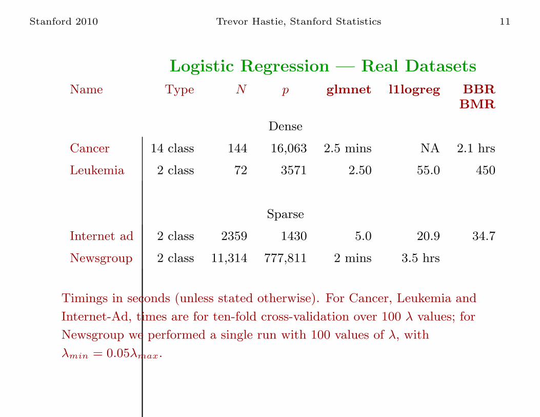
Logistic Regression — Real Datasets
Name Type N p glmnet l1logreg BBR
BMR
Dense
Cancer 14 class 144 16,063 2.5 mins NA 2.1 hrs
Leukemia 2 class 72 3571 2.50 55.0 450
Sparse
Internet ad 2 class 2359 1430 5.0 20.9 34.7
Newsgroup 2 class 11,314 777,811 2 mins 3.5 hrs
Timings in seconds (unless stated otherwise). For Cancer, Leukemia and
Internet-Ad, times are for ten-fold cross-validation over 100 λ values; for
Newsgroup we performed a single run with 100 values of λ, with
λmin = 0.05λmax.

Stanford 2010 Trevor Hastie, Stanford Statistics 12
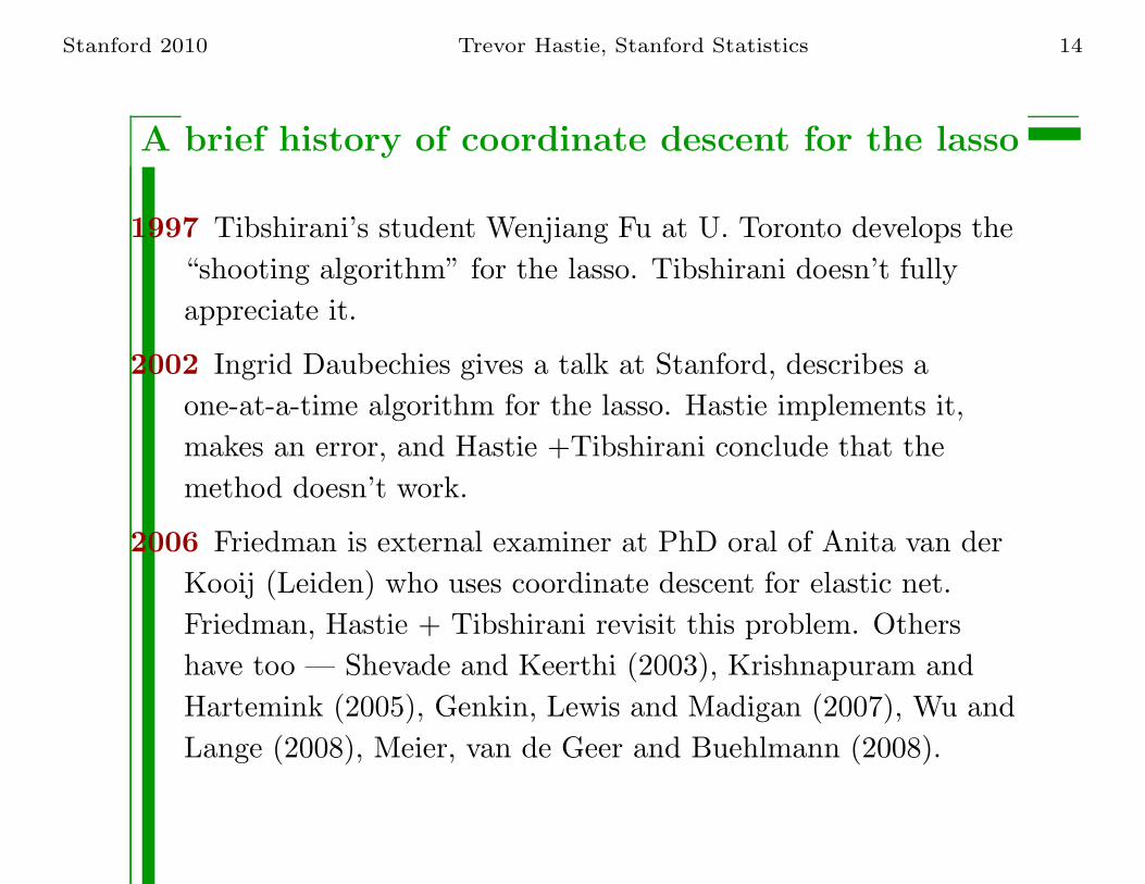
A brief history of coordinate descent for the lasso
1997 Tibshirani’s student Wenjiang Fu at U. Toronto develops the
“shooting algorithm” for the lasso. Tibshirani doesn’t fully
appreciate it.
.
Stanford 2010 Trevor Hastie, Stanford Statistics 13
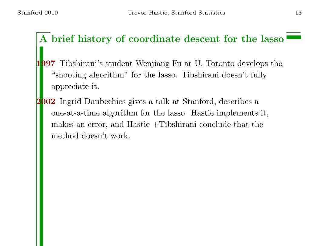
A brief history of coordinate descent for the lasso
1997 Tibshirani’s student Wenjiang Fu at U. Toronto develops the
“shooting algorithm” for the lasso. Tibshirani doesn’t fully
appreciate it.
2002 Ingrid Daubechies gives a talk at Stanford, describes a
one-at-a-time algorithm for the lasso. Hastie implements it,
makes an error, and Hastie +Tibshirani conclude that the
method doesn’t work.
.
Stanford 2010 Trevor Hastie, Stanford Statistics 14
A brief history of coordinate descent for the lasso
1997 Tibshirani’s student Wenjiang Fu at U. Toronto develops the
“shooting algorithm” for the lasso. Tibshirani doesn’t fully
appreciate it.
2002 Ingrid Daubechies gives a talk at Stanford, describes a
one-at-a-time algorithm for the lasso. Hastie implements it,
makes an error, and Hastie +Tibshirani conclude that the
method doesn’t work.
2006 Friedman is external examiner at PhD oral of Anita van der
Kooij (Leiden) who uses coordinate descent for elastic net.
Friedman, Hastie + Tibshirani revisit this problem. Others
have too — Shevade and Keerthi (2003), Krishnapuram and
Hartemink (2005), Genkin, Lewis and Madigan (2007), Wu and
Lange (2008), Meier, van de Geer and Buehlmann (2008).
Stanford 2010 Trevor Hastie, Stanford Statistics 15
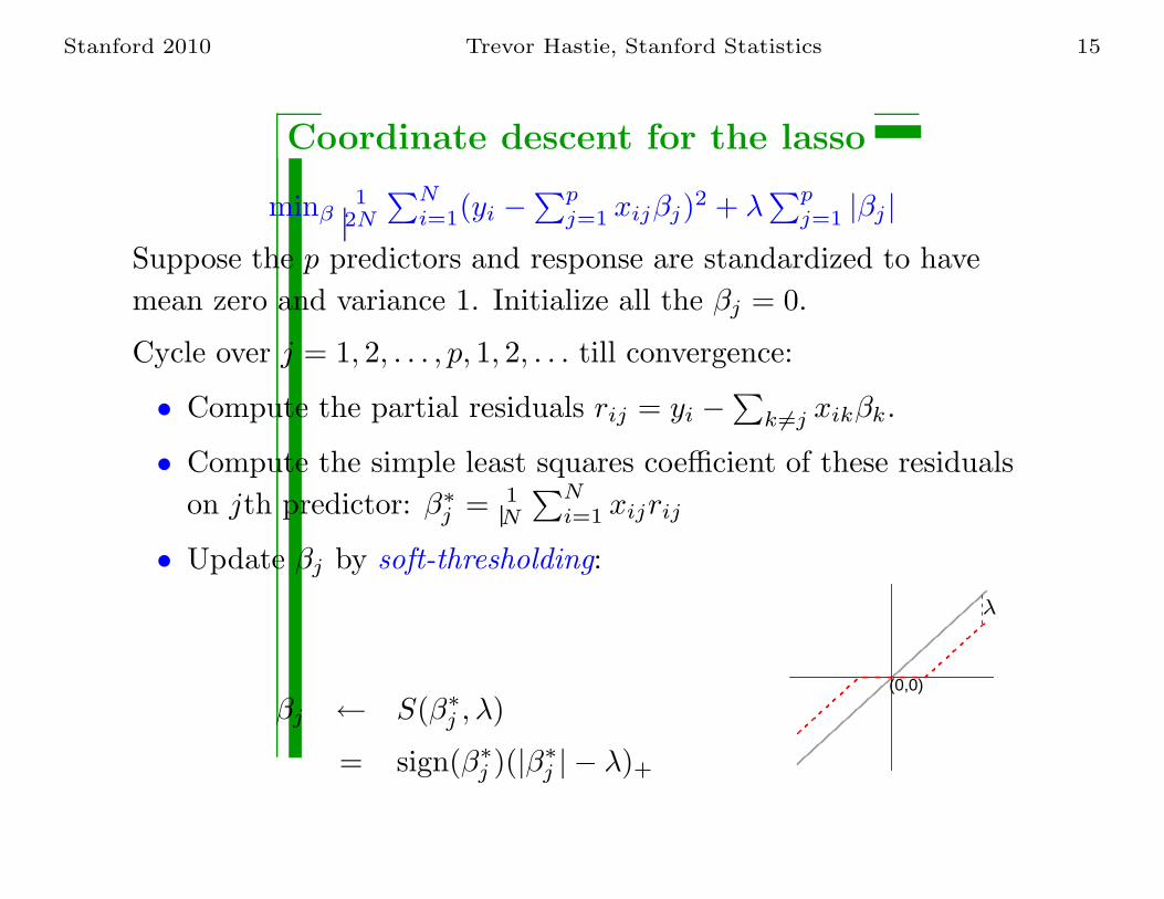
Coordinate descent for the lasso
minβ1
2N
∑Ni=1(yi −
∑pj=1 xijβj)
2 + λ∑p
j=1 |βj |
Suppose the p predictors and response are standardized to have
mean zero and variance 1. Initialize all the βj = 0.
Cycle over j = 1, 2, . . . , p, 1, 2, . . . till convergence:
• Compute the partial residuals rij = yi −∑
k 6=j xikβk.
• Compute the simple least squares coefficient of these residuals
on jth predictor: β∗j = 1
N
∑N
i=1 xijrij
• Update βj by soft-thresholding:
βj ← S(β∗j , λ)
= sign(β∗j )(|β∗
j | − λ)+
(0,0)
λ
Stanford 2010 Trevor Hastie, Stanford Statistics 16
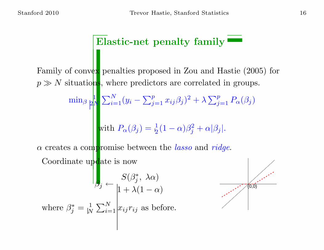
Elastic-net penalty family
Family of convex penalties proposed in Zou and Hastie (2005) for
p≫ N situations, where predictors are correlated in groups.
minβ1
2N
∑Ni=1(yi −
∑pj=1 xijβj)
2 + λ∑p
j=1 Pα(βj)
with Pα(βj) = 12 (1− α)β2
j + α|βj |.
α creates a compromise between the lasso and ridge.
Coordinate update is now
βj ←S(β∗
j , λα)
1 + λ(1− α)
where β∗j = 1
N
∑Ni=1 xijrij as before.
(0,0)

Stanford 2010 Trevor Hastie, Stanford Statistics 17
glmnet: coordinate descent for elastic net family
Friedman, Hastie and Tibshirani 2008
2 4 6 8 10
−0.
10.
00.
10.
20.
3
Step
Coe
ffici
ents
2 4 6 8 10
−0.
10.
00.
10.
20.
3
Step
Coe
ffici
ents
2 4 6 8 10
−0.
10.
00.
10.
20.
3
Step
Coe
ffici
ents
Lasso Elastic Net (0.4) Ridge
Leukemia Data, Logistic regression, N=72, p=3571, first 10 steps shown.
New version of R glmnet package includes Gaussian, Poisson,
Binomial, Multinomial and Cox models.
Stanford 2010 Trevor Hastie, Stanford Statistics 18
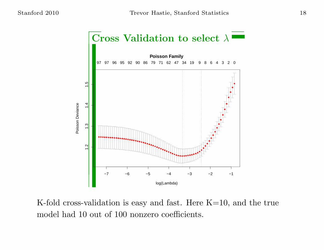
Cross Validation to select λ
−7 −6 −5 −4 −3 −2 −1
1.2
1.3
1.4
1.5
log(Lambda)
Poi
sson
Dev
ianc
e
97 97 96 95 92 90 86 79 71 62 47 34 19 9 8 6 4 3 2 0
Poisson Family
K-fold cross-validation is easy and fast. Here K=10, and the true
model had 10 out of 100 nonzero coefficients.
Stanford 2010 Trevor Hastie, Stanford Statistics 19
Problem with Lasso
When p is large and the number of relevant variables is small:
• to screen out spurious variables, λ should be large, causing bias
in retained variables.
• decreasing λ to reduce bias floods the model with spurious
variables.
Many approaches to modify the lasso to address this problem. Here
we focus on concave penalties.
Stanford 2010 Trevor Hastie, Stanford Statistics 20
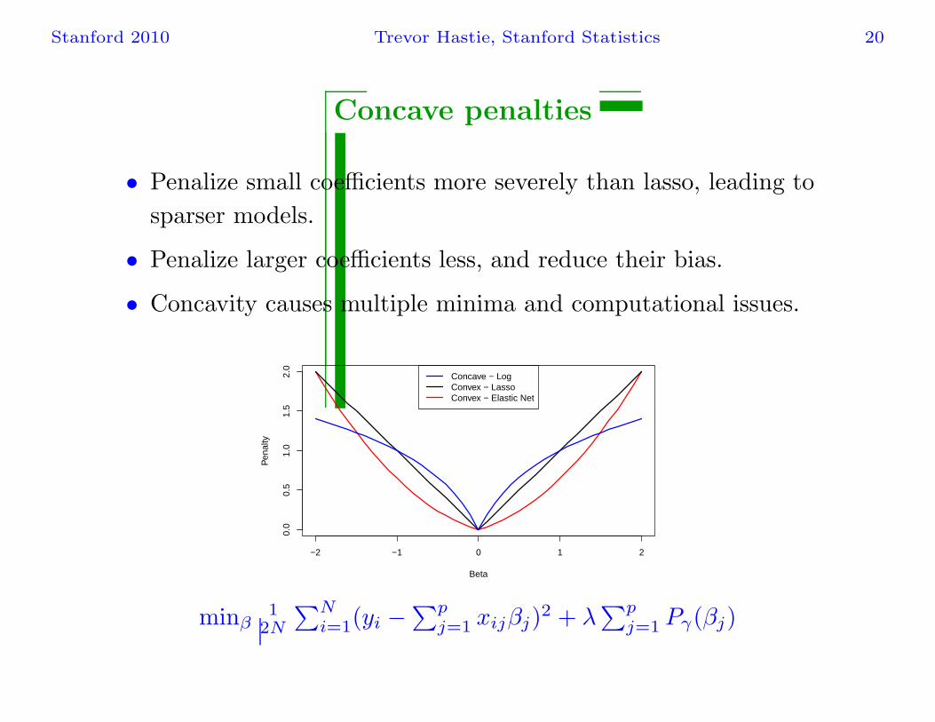
Concave penalties
• Penalize small coefficients more severely than lasso, leading to
sparser models.
• Penalize larger coefficients less, and reduce their bias.
• Concavity causes multiple minima and computational issues.
−2 −1 0 1 2
0.0
0.5
1.0
1.5
2.0
Beta
Pen
alty
Concave − LogConvex − LassoConvex − Elastic Net
minβ1
2N
∑Ni=1(yi −
∑pj=1 xijβj)
2 + λ∑p
j=1 Pγ(βj)
Stanford 2010 Trevor Hastie, Stanford Statistics 21
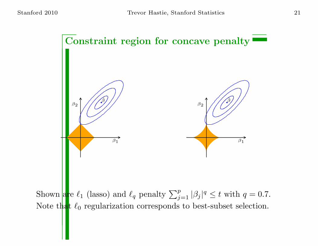
Constraint region for concave penalty
β2
β1
ββ2
β1
β
Shown are ℓ1 (lasso) and ℓq penalty∑p
j=1 |βj |q ≤ t with q = 0.7.
Note that ℓ0 regularization corresponds to best-subset selection.
Stanford 2010 Trevor Hastie, Stanford Statistics 22
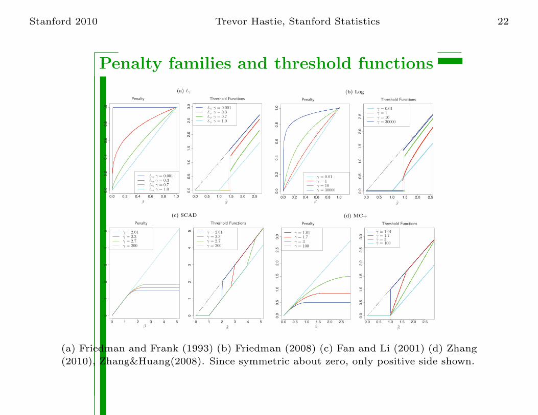
Penalty families and threshold functions
(a) ℓγ
0.0 0.2 0.4 0.6 0.8 1.0
0.0
0.2
0.4
0.6
0.8
1.0
0.0 0.5 1.0 1.5 2.0 2.5
0.0
0.5
1.0
1.5
2.0
2.5
3.0
Penalty Threshold Functions
ℓγ, γ = 0.001
ℓγ, γ = 0.001
ℓγ , γ = 0.3
ℓγ , γ = 0.3
ℓγ , γ = 0.7
ℓγ , γ = 0.7
ℓγ , γ = 1.0
ℓγ , γ = 1.0
β β
(b) Log
0.0 0.2 0.4 0.6 0.8 1.0
0.0
0.2
0.4
0.6
0.8
1.0
0.0 0.5 1.0 1.5 2.0 2.5
0.0
0.5
1.0
1.5
2.0
2.5
Penalty Threshold Functions
β β
γ = 0.01
γ = 0.01
γ = 1
γ = 1
γ = 10
γ = 10
γ = 30000
γ = 30000
(c) SCAD
0 1 2 3 4 5
01
23
45
0 1 2 3 4 5
01
23
45
Penalty Threshold Functions
β β
γ = 2.01γ = 2.01
γ = 2.3γ = 2.3γ = 2.7γ = 2.7γ = 200γ = 200
(d) MC+
0.0 0.5 1.0 1.5 2.0 2.5
0.0
0.5
1.0
1.5
2.0
2.5
3.0
0.0 0.5 1.0 1.5 2.0 2.5
0.0
0.5
1.0
1.5
2.0
2.5
3.0
Penalty Threshold Functions
β β
γ = 1.01γ = 1.01γ = 1.7γ = 1.7γ = 3
γ = 3 γ = 100γ = 100
(a) Friedman and Frank (1993) (b) Friedman (2008) (c) Fan and Li (2001) (d) Zhang
(2010), Zhang&Huang(2008). Since symmetric about zero, only positive side shown.
Stanford 2010 Trevor Hastie, Stanford Statistics 23
sparsenet: coordinate descent for concave families
Mazumder, Friedman and Hastie (2009)
• Start with lasso family and obtain regularization path by
coordinate descent.
• Move down family to slightly concave penalty, using lasso
solutions as warm starts.
• Continue in this fashion till close to best subset penalty.
Results in regularization surface for concave penalty families.
Related ideas in She (2008) using threshold functions, but not coordinate
descent.
Stanford 2010 Trevor Hastie, Stanford Statistics 24
0.0 0.5 1.0 1.5 2.0 2.5 3.0
0.0
0.5
1.0
1.5
2.0
2.5
3.0
0.0 0.5 1.0 1.5 2.0 2.5 3.0
0.0
0.5
1.0
1.5
2.0
2.5
3.0
before calibration after calibration
ββ
γ = 1.01γ = 1.01
γ = 1.7γ = 1.7γ = 3γ = 3
γ = 100γ = 100
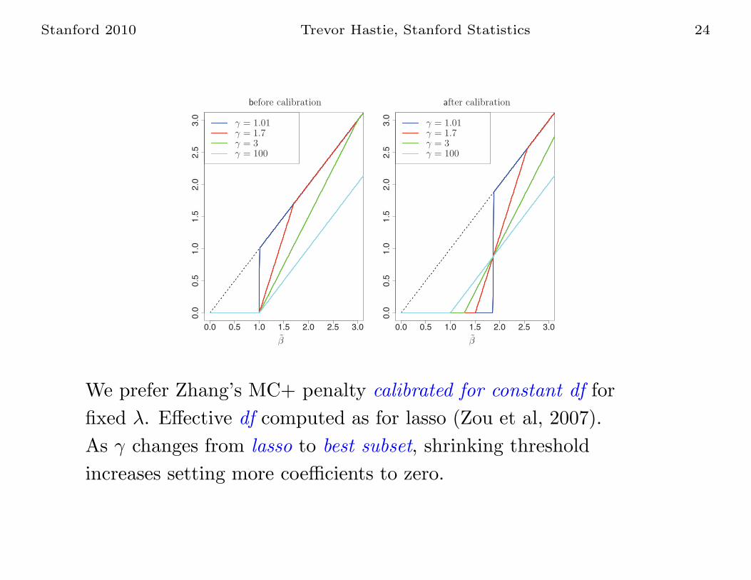
We prefer Zhang’s MC+ penalty calibrated for constant df for
fixed λ. Effective df computed as for lasso (Zou et al, 2007).
As γ changes from lasso to best subset, shrinking threshold
increases setting more coefficients to zero.
Stanford 2010 Trevor Hastie, Stanford Statistics 25
Properties
• Threshold functions are continuous in γ.
• Univariate optimization problems are convex over sufficient
range of γ to cover lasso to subset regression, resulting in
unique coordinate solutions.
• Monotonicity in shrinking threshold.
• Algorithm provably converges to (local) minimum of penalized
objective.
• Empirically outperforms other algorithms for optimizing
concave penalized problems.
• Inherits all theoretical properties of MC+ penalized solutions
(Zhang, 2010, to appear AoS).
Stanford 2010 Trevor Hastie, Stanford Statistics 26
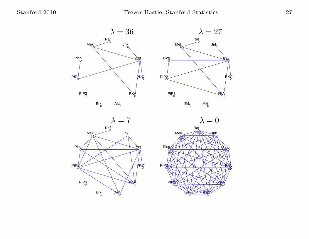
Other Applications using ℓ1 Regularization
Undirected Graphical Models — learning dependence
structure via the lasso. Model the inverse covariance Θ in the
Gaussian family with L1 penalties applied to elements.
maxΘ
log detΘ− Tr(SΘ)− λ||Θ||1
Modified block-wise lasso algorithm, which we solve by
coordinate descent (FHT 2007). Algorithm is very fast, and
solve moderately sparse graphs with 1000 nodes in under a
minute.
Example: flow cytometry - p = 11 proteins measured in N = 7466
cells (Sachs et al 2003) (next page)
Stanford 2010 Trevor Hastie, Stanford Statistics 27
RafMek
Plcg
PIP2
PIP3
Erk Akt
PKA
PKC
P38
JnkRaf
Mek
Plcg
PIP2
PIP3
Erk Akt
PKA
PKC
P38
Jnk
RafMek
Plcg
PIP2
PIP3
Erk Akt
PKA
PKC
P38
JnkRaf
Mek
Plcg
PIP2
PIP3
Erk Akt
PKA
PKC
P38
Jnk
λ = 0λ = 7
λ = 27λ = 36
Stanford 2010 Trevor Hastie, Stanford Statistics 28
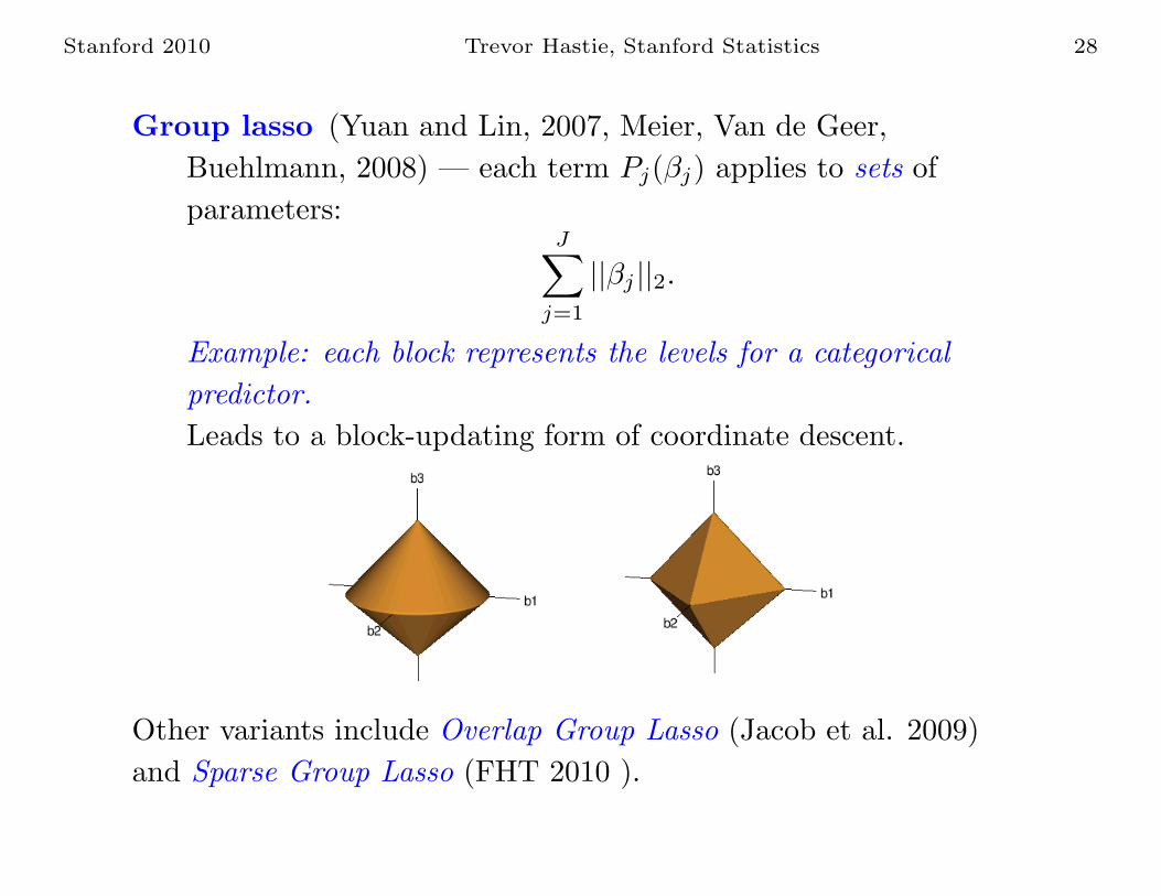
Group lasso (Yuan and Lin, 2007, Meier, Van de Geer,
Buehlmann, 2008) — each term Pj(βj) applies to sets of
parameters:J
∑
j=1
||βj ||2.
Example: each block represents the levels for a categorical
predictor.
Leads to a block-updating form of coordinate descent.
Other variants include Overlap Group Lasso (Jacob et al. 2009)
and Sparse Group Lasso (FHT 2010 ).
Stanford 2010 Trevor Hastie, Stanford Statistics 29
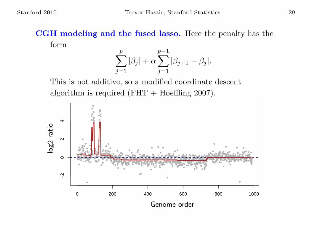
CGH modeling and the fused lasso. Here the penalty has the
formp
∑
j=1
|βj |+ α
p−1∑
j=1
|βj+1 − βj |.
This is not additive, so a modified coordinate descent
algorithm is required (FHT + Hoeffling 2007).
0 200 400 600 800 1000
−2
02
4
Genome order
log2
ratio
Stanford 2010 Trevor Hastie, Stanford Statistics 30
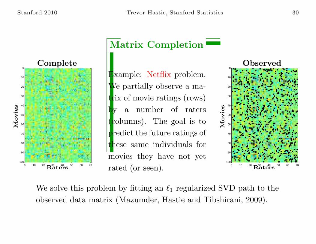
Matrix Completion
0 10 20 30 40 50 60 70
0
10
20
30
40
50
60
70
80
90
100
Complete
Movie
s
Raters
Example: Netflix problem.
We partially observe a ma-
trix of movie ratings (rows)
by a number of raters
(columns). The goal is to
predict the future ratings of
these same individuals for
movies they have not yet
rated (or seen).0 10 20 30 40 50 60 70
0
10
20
30
40
50
60
70
80
90
100
Observed
Movie
s
Raters
We solve this problem by fitting an ℓ1 regularized SVD path to the
observed data matrix (Mazumder, Hastie and Tibshirani, 2009).
Stanford 2010 Trevor Hastie, Stanford Statistics 31
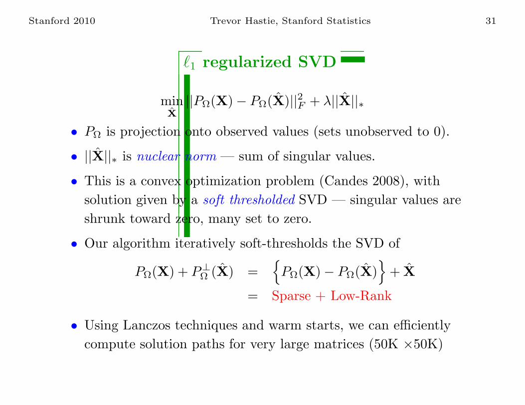
ℓ1 regularized SVD
minX||PΩ(X)− PΩ(X)||2F + λ||X||∗
• PΩ is projection onto observed values (sets unobserved to 0).
• ||X||∗ is nuclear norm — sum of singular values.
• This is a convex optimization problem (Candes 2008), with
solution given by a soft thresholded SVD — singular values are
shrunk toward zero, many set to zero.
• Our algorithm iteratively soft-thresholds the SVD of
PΩ(X) + P⊥Ω (X) =
PΩ(X)− PΩ(X)
+ X
= Sparse + Low-Rank
• Using Lanczos techniques and warm starts, we can efficiently
compute solution paths for very large matrices (50K ×50K)
Stanford 2010 Trevor Hastie, Stanford Statistics 32
Summary
• ℓ1 regularization (and variants) has become a powerful tool
with the advent of wide data.
• Coordinate descent is fastest known algorithm for solving many
of these problems—along a path of values for the tuning
parameter.


![Compression of Deep Convolutional Neural Networks under ... · arXiv:1805.08303v2 [cs.CV] 29 Oct 2018 Compression of Deep Convolutional Neural Networks under Joint Sparsity Constraints](https://static.documents.pub/doc/80x56/5feec481d43bab7eb61c7645/compression-of-deep-convolutional-neural-networks-under-arxiv180508303v2-cscv.jpg)