

Lecture 6:
Association Mapping
Michael Gore lecture notes
Tucson Winter Institute
version 18 Jan 2013

Association Pipeline

Phenotypic Outliers
Outliers are “unusual” data points that
substantially deviate from the mean and
strongly influence parameter estimates
Should ALWAYS check for outliers in
your data sets
Do NOT ignore outliers if detected

Phenotypic Outliers
Outliers can…
1) increase error variance
2) reduce the power of statistical tests
3) distort estimates
4) decrease normality if non-randomly
distributed
“Not all outliers are illegitimate contaminants,
and not all illegitimate scores show up as
outliers.” (Barnett & Lewis, 1994)

Potential Causes of Outliers
Human errors in data collection,
recording, or entry
Technical errors from faulty or
non-calibrated phenotyping equipment
Intentional or motivated mis-reporting
such as “speed” phenotyping in a hot field
environment
Osborne, Jason W. & Amy Overbay (2004)

Phenotyping Tools
Barcoded tools, barcoded tags on plants, barcode
scanners, radio-frequency identification (RFID)
tags, smartphones, hand-held mobile computer…

More Potential Causes of Outliers
Sampling error such as
underrepresentation of a subpopulation
Incorrect assumption about the
distribution (e.g., temporal trend not
accounted for in experimental design)
Real biological outlier – 1% chance of
getting an outlier that is 3 standard
deviations from the mean Osborne, Jason W. & Amy Overbay (2004)

Evaluate Data for Outliers
Histogram
Box-plot (Box and Whisker plot)
Quantile-Quantile plot – graphical
method for comparing two probability
distributions to assess goodness-of-fit
Get to know your data!

Histogram

Box-plot

Box-plot
Center line - median
Central plus sign - mean
25% data
25% data
50% data
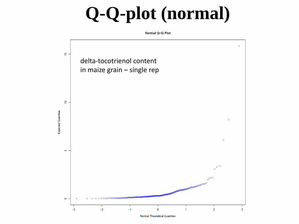
Q-Q-plot (normal)
delta-tocotrienol content in maize grain – single rep

Statistical Identification of Outliers
Cook’s distance – measures influence
of a data point. Data points that
substantially change effect estimates.
Deleted studentized residuals –
measures leverage of a data point. Data
points that affect least squares fit.
Two of several possible methods

Removal of Outliers
Removing anomalous data points from
data sets is controversial to some folks.
My two cents…If outliers are not
removed, inferences made from the fitted
model may not be representative of the
population under study.
If you remove outliers, then be sure to
report it in the manuscript.

Q-Q-plot (normal)
delta-tocotrienol content in maize grain – single rep
Outliers removed based on
deleted studentized residuals

Non-Normal Trait Data
When fitting a mixed model, two very
important assumptions are that the error
terms follow a normal distribution and that
there is a constant variance.
When data are non-normal, these two
assumptions in particular could be
violated.

Analysis of Non-Normal Trait Data
Generalized linear mixed models can
be used to analyze non-normal data
The Box-Cox procedure can be used to
find the most appropriate transformation
that corrects for non-normality of the error
terms and unequal variances.
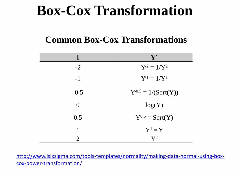
Box-Cox Transformation
Common Box-Cox Transformations
l Y’
-2 Y-2 = 1/Y2
-1 Y-1 = 1/Y1
-0.5 Y-0.5 = 1/(Sqrt(Y))
0 log(Y)
0.5 Y0.5 = Sqrt(Y)
1 Y1 = Y
2 Y2
http://www.isixsigma.com/tools-templates/normality/making-data-normal-using-box-cox-power-transformation/

Q-Q-plot (normal)
delta-tocotrienol content in maize grain – two reps
Outliers removed based on
deleted studentized residuals;
Box-Cox Transformed BLUPs

Association Pipeline

Population structure—allele frequency
differences among individuals due to local
adaptation or diversifying selection
Familial relatedness—allele frequency
differences among individuals due to
recent co-ancestry
If not properly controlled both can cause
spurious associations in GWAS

Fitch-Margoliash tree for 260 maize inbred lines using the log-transformed proportion of
shared alleles distance from 94 SSR markers
Liu et al. 2003 Genetics 165:2117-2128
Maize Population Structure

Structured Association (Q)
A set of random markers is used to
estimate population structure
Estimates are incorporated into a
statistical analysis to control for genetic
structure
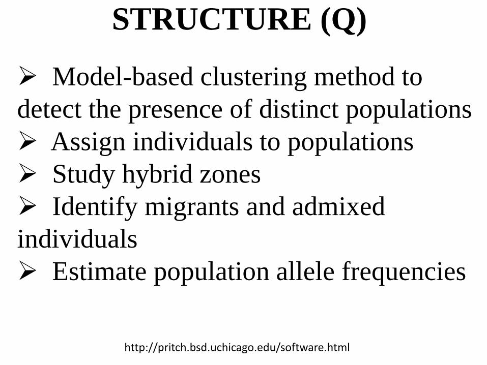
STRUCTURE (Q)
Model-based clustering method to
detect the presence of distinct populations
Assign individuals to populations
Study hybrid zones
Identify migrants and admixed
individuals
Estimate population allele frequencies
http://pritch.bsd.uchicago.edu/software.html
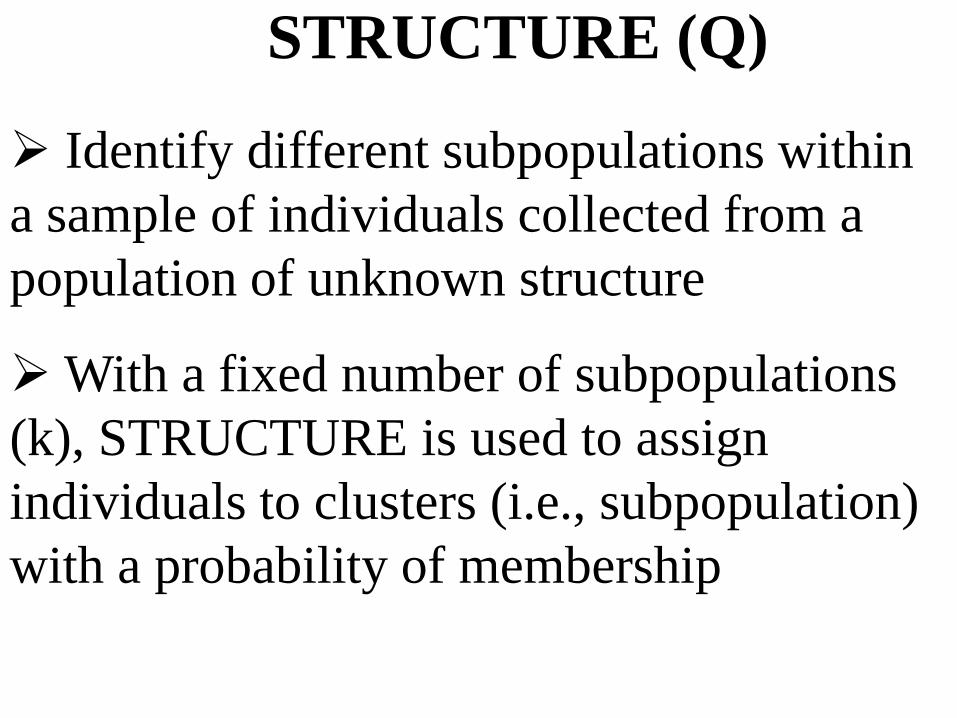
STRUCTURE (Q)
Identify different subpopulations within
a sample of individuals collected from a
population of unknown structure
With a fixed number of subpopulations
(k), STRUCTURE is used to assign
individuals to clusters (i.e., subpopulation)
with a probability of membership

Estimated ln(probability of the data; blue) and Var[ln(probability of
the data; pink)] for k from 2 to 5. Values are from STRUCTURE
run three times at each value of k using 89 SSRs
STRUCTURE (Q)
Hamblin et al. 2007 PLoS ONE 2:e1367
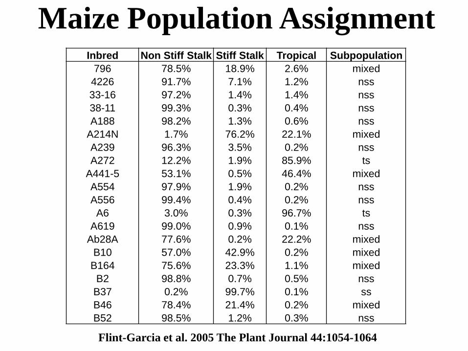
Maize Population AssignmentInbred Non Stiff Stalk Stiff Stalk Tropical Subpopulation
796 78.5% 18.9% 2.6% mixed
4226 91.7% 7.1% 1.2% nss
33-16 97.2% 1.4% 1.4% nss
38-11 99.3% 0.3% 0.4% nss
A188 98.2% 1.3% 0.6% nss
A214N 1.7% 76.2% 22.1% mixed
A239 96.3% 3.5% 0.2% nss
A272 12.2% 1.9% 85.9% ts
A441-5 53.1% 0.5% 46.4% mixed
A554 97.9% 1.9% 0.2% nss
A556 99.4% 0.4% 0.2% nss
A6 3.0% 0.3% 96.7% ts
A619 99.0% 0.9% 0.1% nss
Ab28A 77.6% 0.2% 22.2% mixed
B10 57.0% 42.9% 0.2% mixed
B164 75.6% 23.3% 1.1% mixed
B2 98.8% 0.7% 0.5% nss
B37 0.2% 99.7% 0.1% ss
B46 78.4% 21.4% 0.2% mixed
B52 98.5% 1.2% 0.3% nss
Flint-Garcia et al. 2005 The Plant Journal 44:1054-1064

STRUCTURE (Q)
Determination of the number of subpopulations k based on
STRUCTURE and 359 SSR markers using the ad hoc
criterion Δ K of Evanno et al. 2005 Mol. Ecol. 14:2611-2620
Van Inghelandt et al. 2010 Theoretical Applied Genetics 120:1289-1299

Principle Component Analysis
Fast and effective approach to
diagnose population structure
PCA summarizes variation observed
across all markers into a smaller
number of underlying component
variables

Principle Component Analysis
PCs relate to separate, unobserved
subpopulations from which genotyped
individuals originated
Loading of each individual on each
PC describe population membership

Principle Component Analysis
EINGENSTRAT software package is used
to estimate PCs of the marker data

Principle Component Analysis
Scree plot –
shows the
fraction of total
variance in the
data explained
by each PC

A kinship coefficient (F) is the
probability that two homologous genes are
identical by descent
Kinship from genetic markers is an
estimate of relative kinship that is based
on probabilities of identical by state
Even with pedigrees, marker-based
kinship has higher accuracy
Kinship Coefficient (K)

Marker-based Relative Kinship (K)
Fij = (Qij-Qm)/(1-Qm) ≅ Θij ,
where Qij is the probability of identity by state
for random genes from i and j, and Qm is the
average probability of identity by state for
genes coming from random individuals in the
population from which i and j where drawn.

SPAGeDi software package with
Loiselle (Loiselle et al., 1995) kinship
coefficient can be used to generate the
relative kinship matrix
Negative values between individuals
should be set to zero. These individuals
are less related than random individuals
(i.e., degree of genetic covariance caused
by polygenic effects is defined to be 0)
Marker-based Relative Kinship (K)

The original kinship matrix for mixed
models is an additive numerator
relationship matrix calculated from
pedigree
Diagonals have values between 1 and 2
(1 plus inbreeding coefficient) and off
diagonals have values between 0 and 1
(kinship)
Marker-based Relative Kinship (K)
Therefore, A-matrix is twice the co-
ancestry matrix used in population
genetics
Multiplication of K by 2 for inbred
lines does not change BLUEs and
BLUPs but affects the ratios of VC
estimates
Marker-based Relative Kinship (K)

Number of Background Markers
Needed for Estimating Relationships
Yu et al. 2009 The Plant Genome 2:63-77
Likelihood-based model fitting can be
used to quantify robustness of genetic
relatedness derived from markers
Kinship is more sensitive than
population structure to marker number
Number of Background Markers
Needed for Estimating Relationships
Yu et al. 2009 The Plant Genome 2:63-77
Robustness of relationship estimate can
be tested by fitting multiple phenotypic
traits with different subsets of markers
Number required for biallelic SNPs is
higher than multiallelic SSRs (e.g., maize
– 100 SSRs; 1000 SNPs)

Model Fit with the Mixed Model
Bayesian information criterion (BIC)
can be used to determine the optimal
number of principal components to
include in the GWAS model
The goodness-of-fit among GWAS
models can be assessed with a likelihood-
ratio-based R2 statistic, denoted R2LR
Sun et al. 2010 Heredity 105:333-340

Model Fit with the Mixed Model
R2LR considers the change of likelihood
between models with different fixed and
random effects
R2LR is easily computed and has a
monotonic nondecreasing property
Sun et al. 2010 Heredity 105:333-340

Computation with Mixed Models
Large numbers of individuals is
computationally intensive for mixed
models
Computing time for solving MLM
increases with the cube of the number of
individuals fit as a random effect
Computing time is further increased
because iteration is needed to estimate
parameters such as variance components
Zhang et al. 2010 Nature Genetics 42:355-360
Efficient Computation
Compression – reduce the size of the
random genetic effect in the absence of
pedigree information by clustering
individuals into groups
Population parameters previously
determined (P3D) – eliminate iterations to
re-estimate variance components for each
marker

Zhang et al. 2010 Nature Genetics 42:355-360
Compression and P3D
The joint use of compression MLM and
P3D greatly reduces computing time and
maintains or increases statistical power
no compression, no P3D – GWAS with
1,315 individuals and 1 million markers
takes 26 years
compression with P3D – takes 2.7 days
for GWAS with the same data set

Correcting for Multiple Testing
Bonferroni correction – procedure to
control the family-wise error rate (i.e.,
probability of making one or more type I
errors)
Simplest and most conservative method
to control FWER
Calculated as α/n, when n is number of
hypotheses (i.e., SNPs tested)

Correcting for Multiple Testing
False Discovery Rate– procedure to
control the expected proportion of false
discoveries
Less stringent than Bonferroni
q-value is the FDR analogue of p-value
e.g., q=0.10 is 10 false discoveries/100 tests
Benjamini–Hochberg procedure is often
used in GWAS
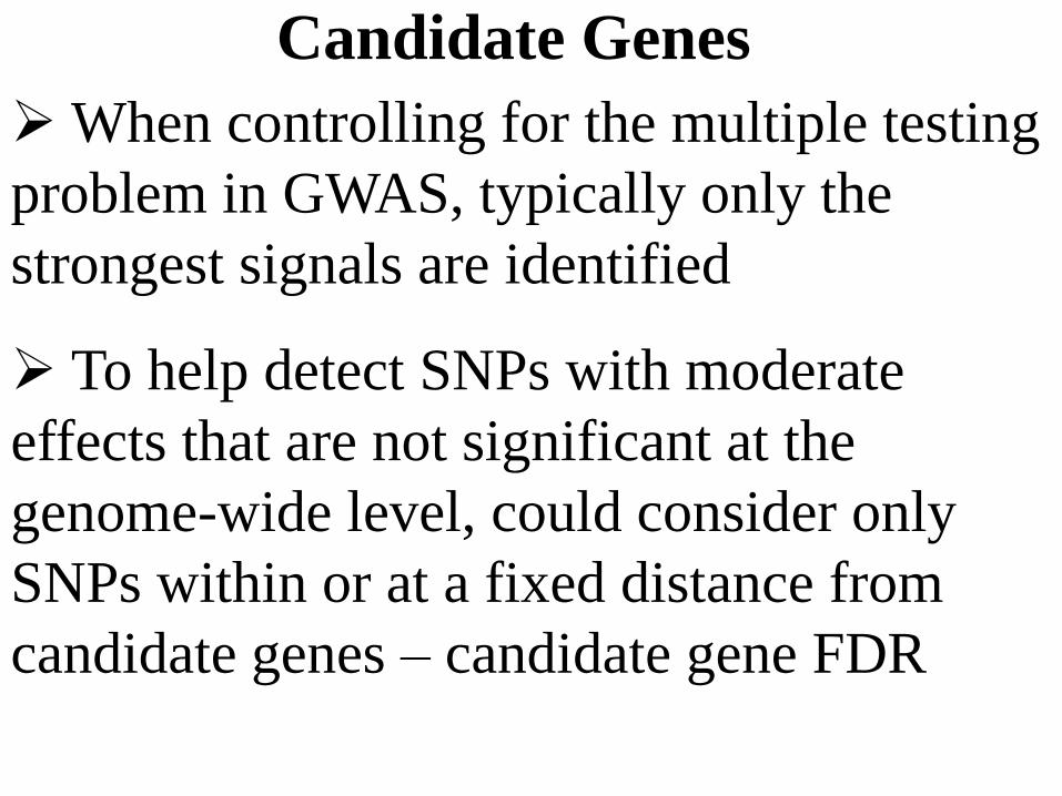
Candidate Genes
When controlling for the multiple testing
problem in GWAS, typically only the
strongest signals are identified
To help detect SNPs with moderate
effects that are not significant at the
genome-wide level, could consider only
SNPs within or at a fixed distance from
candidate genes – candidate gene FDR
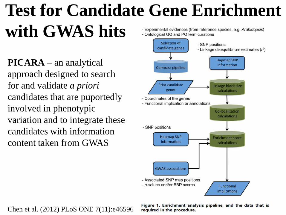
Test for Candidate Gene Enrichment
with GWAS hits
PICARA – an analytical
approach designed to search
for and validate a priori
candidates that are puportedly
involved in phenotypic
variation and to integrate these
candidates with information
content taken from GWAS
Chen et al. (2012) PLoS ONE 7(11):e46596

Rare Variants in GWAS
GWAS typically identify common
variants but rare variants are important
Most NGS-GWAS are severely
underpowered for testing rare variants
SNPs with a very low MAF (<0.05) may
not have Type I error rates at nominal levels
Need very large sample sizes

Rare Variant GWAS Methods
Power of single marker tests is poor, thus
collapsing rare variants across a region
creates a more common aggregate (Li and
Leal, 2008).
Weighting of alleles on criteria such as
MAF or biological function (Madsen and
Browning, 2009)
Ladouceur et al. (2012) The Empirical Power of Rare Variant Association Methods:
Results from Sanger Sequencing in 1,998 Individuals. PLoS Genet 8: e1002496
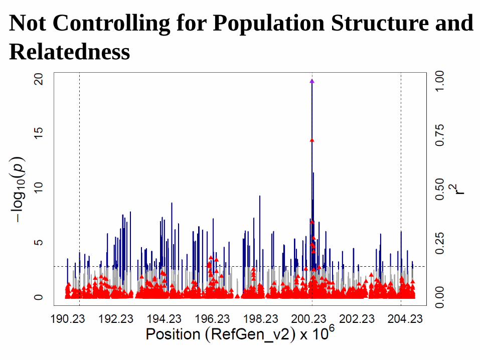
Not Controlling for Population Structure and
Relatedness

Controlling for Population Structure and
Relatedness
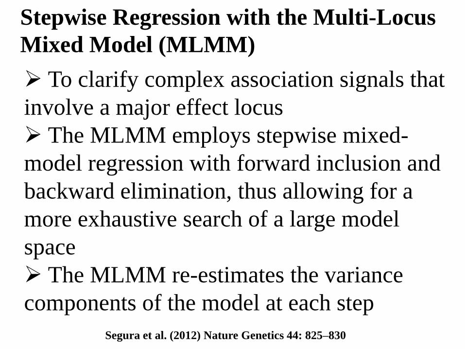
Stepwise Regression with the Multi-Locus
Mixed Model (MLMM)
Segura et al. (2012) Nature Genetics 44: 825–830
To clarify complex association signals that
involve a major effect locus
The MLMM employs stepwise mixed-
model regression with forward inclusion and
backward elimination, thus allowing for a
more exhaustive search of a large model
space
The MLMM re-estimates the variance
components of the model at each step
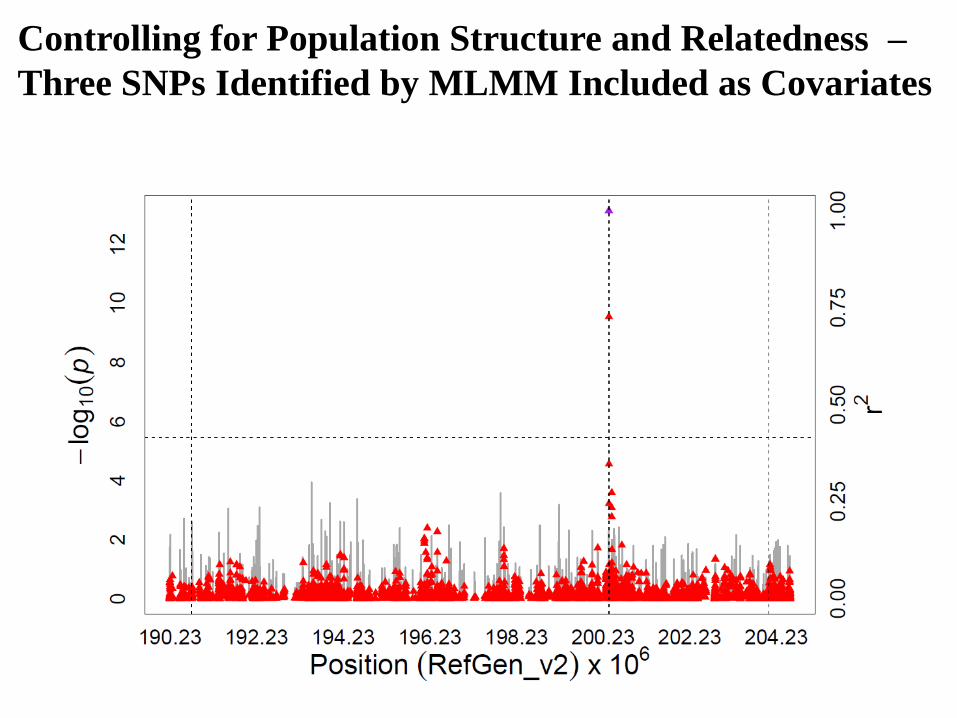
Controlling for Population Structure and Relatedness –
Three SNPs Identified by MLMM Included as Covariates
Software for Genome-Wide Association and
Genomic Selection
http://www.maizegenetics.net/gapit
GAPIT - Genome Association and Prediction Integrated Tool
TASSEL - Trait Analysis by aSSociation, Evolution and Linkage
http://www.maizegenetics.net/bioinformatics


