
Lecture 6: Value Function Approximation
Lecture 6: Value Function Approximation
David Silver

Lecture 6: Value Function Approximation
Outline
1 Introduction
2 Incremental Methods
3 Batch Methods
Lecture 6: Value Function Approximation
Introduction
Outline
1 Introduction
2 Incremental Methods
3 Batch Methods

Lecture 6: Value Function Approximation
Introduction
Large-Scale Reinforcement Learning
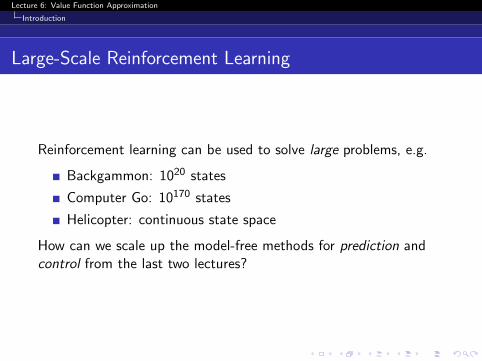
Reinforcement learning can be used to solve large problems, e.g.
Backgammon: 1020 states
Computer Go: 10170 states
Helicopter: continuous state space
How can we scale up the model-free methods for prediction andcontrol from the last two lectures?
Lecture 6: Value Function Approximation
Introduction
Large-Scale Reinforcement Learning
Reinforcement learning can be used to solve large problems, e.g.
Backgammon: 1020 states
Computer Go: 10170 states
Helicopter: continuous state space
How can we scale up the model-free methods for prediction andcontrol from the last two lectures?
Lecture 6: Value Function Approximation
Introduction
Value Function Approximation
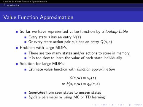
So far we have represented value function by a lookup table
Every state s has an entry V (s)Or every state-action pair s, a has an entry Q(s, a)
Problem with large MDPs:
There are too many states and/or actions to store in memoryIt is too slow to learn the value of each state individually
Solution for large MDPs:
Estimate value function with function approximation
v̂(s,w) ≈ vπ(s)
or q̂(s, a,w) ≈ qπ(s, a)
Generalise from seen states to unseen statesUpdate parameter w using MC or TD learning

Lecture 6: Value Function Approximation
Introduction
Types of Value Function Approximation
s s sa
v(s,w) q(s,a,w) q(s,a1,w) q(s,am,w)…
w w w
^ ^ ^ ^
Lecture 6: Value Function Approximation
Introduction
Which Function Approximator?
There are many function approximators, e.g.
Linear combinations of features
Neural network
Decision tree
Nearest neighbour
Fourier / wavelet bases
...

Lecture 6: Value Function Approximation
Introduction
Which Function Approximator?
We consider differentiable function approximators, e.g.
Linear combinations of features
Neural network
Decision tree
Nearest neighbour
Fourier / wavelet bases
...
Furthermore, we require a training method that is suitable fornon-stationary, non-iid data
Lecture 6: Value Function Approximation
Incremental Methods
Outline
1 Introduction
2 Incremental Methods
3 Batch Methods

Lecture 6: Value Function Approximation
Incremental Methods
Gradient Descent
Gradient Descent
Let J(w) be a differentiable function ofparameter vector w
Define the gradient of J(w) to be
∇wJ(w) =
∂J(w)∂w1
...∂J(w)∂wn
To find a local minimum of J(w)
Adjust w in direction of -ve gradient
∆w = −1
2α∇wJ(w)
where α is a step-size parameter
!"#$%"&'(%")*+,#'-'!"#$%%" (%")*+,#'.+/0+,#
!"#$%&'('%$&#()&*+$,*$#&&-&$$$$."'%"$'*$%-/0'*,('-*$.'("$("#$1)*%('-*$,22&-3'/,(-& %,*$0#$)+#4$(-$%&#,(#$,*$#&&-&$1)*%('-*$$$$$$$$$$$$$
!"#$2,&(',5$4'11#&#*(',5$-1$("'+$#&&-&$1)*%('-*$$$$$$$$$$$$$$$$6$("#$7&,4'#*($%,*$*-.$0#$)+#4$(-$)24,(#$("#$'*(#&*,5$8,&',05#+$'*$("#$1)*%('-*$,22&-3'/,(-& 9,*4$%&'('%:;$$$$$$
<&,4'#*($4#+%#*($=>?
Lecture 6: Value Function Approximation
Incremental Methods
Gradient Descent
Value Function Approx. By Stochastic Gradient Descent
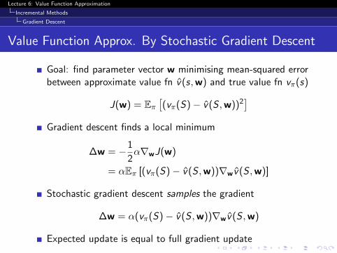
Goal: find parameter vector w minimising mean-squared errorbetween approximate value fn v̂(s,w) and true value fn vπ(s)
J(w) = Eπ[(vπ(S)− v̂(S ,w))2
]Gradient descent finds a local minimum
∆w = −1
2α∇wJ(w)
= αEπ [(vπ(S)− v̂(S ,w))∇wv̂(S ,w)]
Stochastic gradient descent samples the gradient
∆w = α(vπ(S)− v̂(S ,w))∇wv̂(S ,w)
Expected update is equal to full gradient update
Lecture 6: Value Function Approximation
Incremental Methods
Linear Function Approximation
Feature Vectors
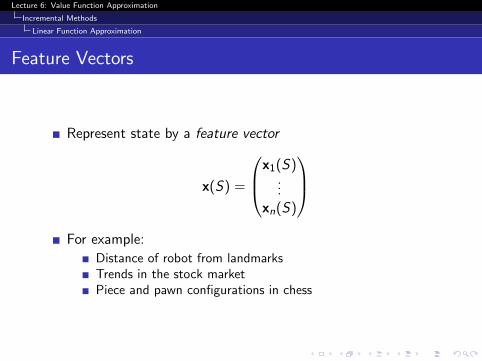
Represent state by a feature vector
x(S) =
x1(S)...
xn(S)
For example:
Distance of robot from landmarksTrends in the stock marketPiece and pawn configurations in chess

Lecture 6: Value Function Approximation
Incremental Methods
Linear Function Approximation
Linear Value Function Approximation
Represent value function by a linear combination of features
v̂(S ,w) = x(S)>w =n∑
j=1
xj(S)wj
Objective function is quadratic in parameters w
J(w) = Eπ[(vπ(S)− x(S)>w)2
]Stochastic gradient descent converges on global optimum
Update rule is particularly simple
∇wv̂(S ,w) = x(S)
∆w = α(vπ(S)− v̂(S ,w))x(S)
Update = step-size × prediction error × feature value
Lecture 6: Value Function Approximation
Incremental Methods
Linear Function Approximation
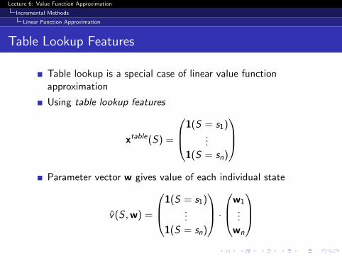
Table Lookup Features
Table lookup is a special case of linear value functionapproximation
Using table lookup features
xtable(S) =
1(S = s1)...
1(S = sn)
Parameter vector w gives value of each individual state
v̂(S ,w) =
1(S = s1)...
1(S = sn)
·w1
...wn

Lecture 6: Value Function Approximation
Incremental Methods
Incremental Prediction Algorithms
Incremental Prediction Algorithms
Have assumed true value function vπ(s) given by supervisor
But in RL there is no supervisor, only rewards
In practice, we substitute a target for vπ(s)
For MC, the target is the return Gt
∆w = α(Gt − v̂(St ,w))∇wv̂(St ,w)
For TD(0), the target is the TD target Rt+1 + γv̂(St+1,w)
∆w = α(Rt+1 + γv̂(St+1,w)− v̂(St ,w))∇wv̂(St ,w)
For TD(λ), the target is the λ-return Gλt
∆w = α(Gλt − v̂(St ,w))∇wv̂(St ,w)
Lecture 6: Value Function Approximation
Incremental Methods
Incremental Prediction Algorithms
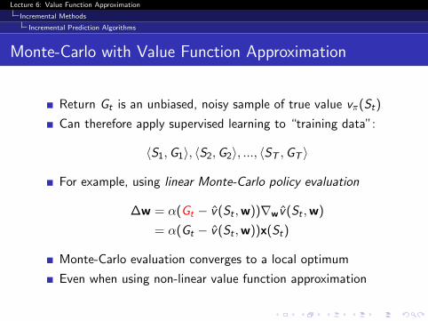
Monte-Carlo with Value Function Approximation
Return Gt is an unbiased, noisy sample of true value vπ(St)
Can therefore apply supervised learning to “training data”:
〈S1,G1〉, 〈S2,G2〉, ..., 〈ST ,GT 〉
For example, using linear Monte-Carlo policy evaluation
∆w = α(Gt − v̂(St ,w))∇wv̂(St ,w)
= α(Gt − v̂(St ,w))x(St)
Monte-Carlo evaluation converges to a local optimum
Even when using non-linear value function approximation
Lecture 6: Value Function Approximation
Incremental Methods
Incremental Prediction Algorithms
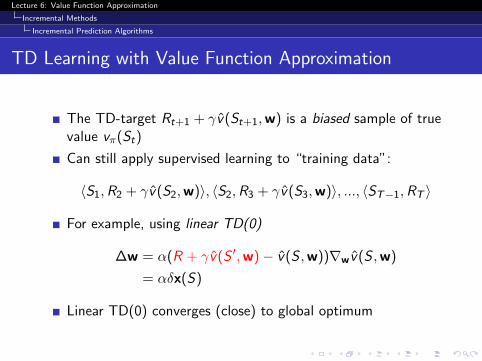
TD Learning with Value Function Approximation
The TD-target Rt+1 + γv̂(St+1,w) is a biased sample of truevalue vπ(St)
Can still apply supervised learning to “training data”:
〈S1,R2 + γv̂(S2,w)〉, 〈S2,R3 + γv̂(S3,w)〉, ..., 〈ST−1,RT 〉
For example, using linear TD(0)
∆w = α(R + γv̂(S ′,w)− v̂(S ,w))∇wv̂(S ,w)
= αδx(S)
Linear TD(0) converges (close) to global optimum
Lecture 6: Value Function Approximation
Incremental Methods
Incremental Prediction Algorithms
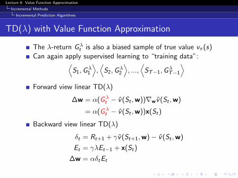
TD(λ) with Value Function Approximation
The λ-return Gλt is also a biased sample of true value vπ(s)
Can again apply supervised learning to “training data”:⟨S1,G
λ1
⟩,⟨S2,G
λ2
⟩, ...,
⟨ST−1,G
λT−1
⟩Forward view linear TD(λ)
∆w = α(Gλt − v̂(St ,w))∇wv̂(St ,w)
= α(Gλt − v̂(St ,w))x(St)
Backward view linear TD(λ)
δt = Rt+1 + γv̂(St+1,w)− v̂(St ,w)
Et = γλEt−1 + x(St)
∆w = αδtEt
Forward view and backward view linear TD(λ) are equivalent

Lecture 6: Value Function Approximation
Incremental Methods
Incremental Prediction Algorithms
TD(λ) with Value Function Approximation
The λ-return Gλt is also a biased sample of true value vπ(s)
Can again apply supervised learning to “training data”:⟨S1,G
λ1
⟩,⟨S2,G
λ2
⟩, ...,
⟨ST−1,G
λT−1
⟩Forward view linear TD(λ)
∆w = α(Gλt − v̂(St ,w))∇wv̂(St ,w)
= α(Gλt − v̂(St ,w))x(St)
Backward view linear TD(λ)
δt = Rt+1 + γv̂(St+1,w)− v̂(St ,w)
Et = γλEt−1 + x(St)
∆w = αδtEt
Forward view and backward view linear TD(λ) are equivalent
Lecture 6: Value Function Approximation
Incremental Methods
Incremental Control Algorithms
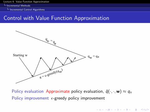
Control with Value Function Approximation
qw = qπ
Starting w
π = ε-greedy(q w)
qw ≈ q*
Policy evaluation Approximate policy evaluation, q̂(·, ·,w) ≈ qπ
Policy improvement ε-greedy policy improvement

Lecture 6: Value Function Approximation
Incremental Methods
Incremental Control Algorithms
Action-Value Function Approximation
Approximate the action-value function
q̂(S ,A,w) ≈ qπ(S ,A)
Minimise mean-squared error between approximateaction-value fn q̂(S ,A,w) and true action-value fn qπ(S ,A)
J(w) = Eπ[(qπ(S ,A)− q̂(S ,A,w))2
]Use stochastic gradient descent to find a local minimum
−1
2∇wJ(w) = (qπ(S ,A)− q̂(S ,A,w))∇wq̂(S ,A,w)
∆w = α(qπ(S ,A)− q̂(S ,A,w))∇wq̂(S ,A,w)
Lecture 6: Value Function Approximation
Incremental Methods
Incremental Control Algorithms
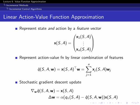
Linear Action-Value Function Approximation
Represent state and action by a feature vector
x(S ,A) =
x1(S ,A)...
xn(S ,A)
Represent action-value fn by linear combination of features
q̂(S ,A,w) = x(S ,A)>w =n∑
j=1
xj(S ,A)wj
Stochastic gradient descent update
∇wq̂(S ,A,w) = x(S ,A)
∆w = α(qπ(S ,A)− q̂(S ,A,w))x(S ,A)

Lecture 6: Value Function Approximation
Incremental Methods
Incremental Control Algorithms
Incremental Control Algorithms
Like prediction, we must substitute a target for qπ(S ,A)For MC, the target is the return Gt
∆w = α(Gt − q̂(St ,At ,w))∇wq̂(St ,At ,w)
For TD(0), the target is the TD target Rt+1 + γQ(St+1,At+1)
∆w = α(Rt+1 + γq̂(St+1,At+1,w)− q̂(St ,At ,w))∇wq̂(St ,At ,w)
For forward-view TD(λ), target is the action-value λ-return
∆w = α(qλt − q̂(St ,At ,w))∇wq̂(St ,At ,w)
For backward-view TD(λ), equivalent update is
δt = Rt+1 + γq̂(St+1,At+1,w)− q̂(St ,At ,w)
Et = γλEt−1 +∇wq̂(St ,At ,w)
∆w = αδtEt

Lecture 6: Value Function Approximation
Incremental Methods
Mountain Car
Linear Sarsa with Coarse Coding in Mountain Car

Lecture 6: Value Function Approximation
Incremental Methods
Mountain Car
Linear Sarsa with Radial Basis Functions in Mountain Car
Lecture 6: Value Function Approximation
Incremental Methods
Mountain Car
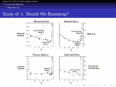
Study of λ: Should We Bootstrap?
Lecture 6: Value Function Approximation
Incremental Methods
Convergence
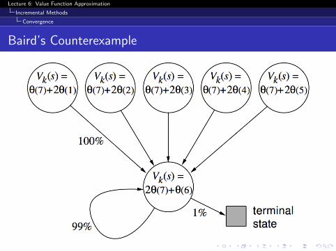
Baird’s Counterexample
Lecture 6: Value Function Approximation
Incremental Methods
Convergence
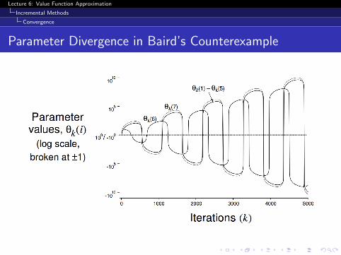
Parameter Divergence in Baird’s Counterexample

Lecture 6: Value Function Approximation
Incremental Methods
Convergence
Convergence of Prediction Algorithms
On/Off-Policy Algorithm Table Lookup Linear Non-Linear
On-PolicyMC 3 3 3
TD(0) 3 3 7
TD(λ) 3 3 7
Off-PolicyMC 3 3 3
TD(0) 3 7 7
TD(λ) 3 7 7
Lecture 6: Value Function Approximation
Incremental Methods
Convergence
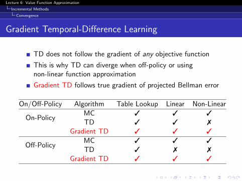
Gradient Temporal-Difference Learning
TD does not follow the gradient of any objective function
This is why TD can diverge when off-policy or usingnon-linear function approximation
Gradient TD follows true gradient of projected Bellman error
On/Off-Policy Algorithm Table Lookup Linear Non-Linear
On-PolicyMC 3 3 3
TD 3 3 7
Gradient TD 3 3 3
Off-PolicyMC 3 3 3
TD 3 7 7
Gradient TD 3 3 3
Lecture 6: Value Function Approximation
Incremental Methods
Convergence
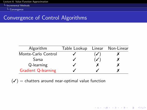
Convergence of Control Algorithms
Algorithm Table Lookup Linear Non-Linear
Monte-Carlo Control 3 (3) 7
Sarsa 3 (3) 7
Q-learning 3 7 7
Gradient Q-learning 3 3 7
(3) = chatters around near-optimal value function
Lecture 6: Value Function Approximation
Batch Methods
Outline
1 Introduction
2 Incremental Methods
3 Batch Methods

Lecture 6: Value Function Approximation
Batch Methods
Batch Reinforcement Learning
Gradient descent is simple and appealing
But it is not sample efficient
Batch methods seek to find the best fitting value function
Given the agent’s experience (“training data”)

Lecture 6: Value Function Approximation
Batch Methods
Least Squares Prediction
Least Squares Prediction
Given value function approximation v̂(s,w) ≈ vπ(s)
And experience D consisting of 〈state, value〉 pairs
D = {〈s1, vπ1 〉, 〈s2, vπ2 〉, ..., 〈sT , vπT 〉}
Which parameters w give the best fitting value fn v̂(s,w)?
Least squares algorithms find parameter vector w minimisingsum-squared error between v̂(st ,w) and target values vπt ,
LS(w) =T∑t=1
(vπt − v̂(st ,w))2
= ED[(vπ − v̂(s,w))2
]

Lecture 6: Value Function Approximation
Batch Methods
Least Squares Prediction
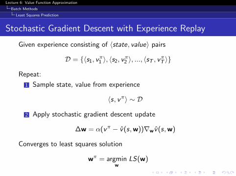
Stochastic Gradient Descent with Experience Replay
Given experience consisting of 〈state, value〉 pairs
D = {〈s1, vπ1 〉, 〈s2, vπ2 〉, ..., 〈sT , vπT 〉}
Repeat:
1 Sample state, value from experience
〈s, vπ〉 ∼ D
2 Apply stochastic gradient descent update
∆w = α(vπ − v̂(s,w))∇wv̂(s,w)
Converges to least squares solution
wπ = argminw
LS(w)
Lecture 6: Value Function Approximation
Batch Methods
Least Squares Prediction
Stochastic Gradient Descent with Experience Replay
Given experience consisting of 〈state, value〉 pairs
D = {〈s1, vπ1 〉, 〈s2, vπ2 〉, ..., 〈sT , vπT 〉}
Repeat:
1 Sample state, value from experience
〈s, vπ〉 ∼ D
2 Apply stochastic gradient descent update
∆w = α(vπ − v̂(s,w))∇wv̂(s,w)
Converges to least squares solution
wπ = argminw
LS(w)

Lecture 6: Value Function Approximation
Batch Methods
Least Squares Prediction
Experience Replay in Deep Q-Networks (DQN)
DQN uses experience replay and fixed Q-targets
Take action at according to ε-greedy policy
Store transition (st , at , rt+1, st+1) in replay memory DSample random mini-batch of transitions (s, a, r , s ′) from DCompute Q-learning targets w.r.t. old, fixed parameters w−
Optimise MSE between Q-network and Q-learning targets
Li (wi ) = Es,a,r ,s′∼Di
[(r + γ max
a′Q(s ′, a′;w−i )− Q(s, a;wi )
)2]
Using variant of stochastic gradient descent

Lecture 6: Value Function Approximation
Batch Methods
Least Squares Prediction
DQN in Atari
End-to-end learning of values Q(s, a) from pixels s
Input state s is stack of raw pixels from last 4 frames
Output is Q(s, a) for 18 joystick/button positions
Reward is change in score for that step
Network architecture and hyperparameters fixed across all games

Lecture 6: Value Function Approximation
Batch Methods
Least Squares Prediction
DQN Results in Atari

Lecture 6: Value Function Approximation
Batch Methods
Least Squares Prediction
How much does DQN help?
Replay Replay No replay No replayFixed-Q Q-learning Fixed-Q Q-learning
Breakout 316.81 240.73 10.16 3.17
Enduro 1006.3 831.25 141.89 29.1
River Raid 7446.62 4102.81 2867.66 1453.02
Seaquest 2894.4 822.55 1003 275.81
Space Invaders 1088.94 826.33 373.22 301.99

Lecture 6: Value Function Approximation
Batch Methods
Least Squares Prediction
Linear Least Squares Prediction
Experience replay finds least squares solution
But it may take many iterations
Using linear value function approximation v̂(s,w) = x(s)>w
We can solve the least squares solution directly
Lecture 6: Value Function Approximation
Batch Methods
Least Squares Prediction
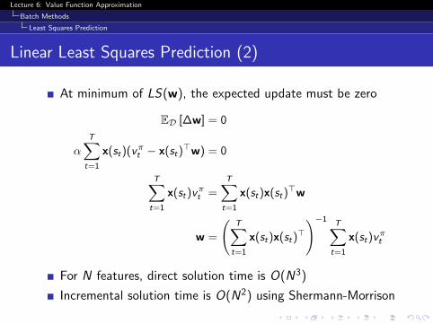
Linear Least Squares Prediction (2)
At minimum of LS(w), the expected update must be zero
ED [∆w] = 0
α
T∑t=1
x(st)(vπt − x(st)
>w) = 0
T∑t=1
x(st)vπt =
T∑t=1
x(st)x(st)>w
w =
(T∑t=1
x(st)x(st)>
)−1 T∑t=1
x(st)vπt
For N features, direct solution time is O(N3)
Incremental solution time is O(N2) using Shermann-Morrison
Lecture 6: Value Function Approximation
Batch Methods
Least Squares Prediction
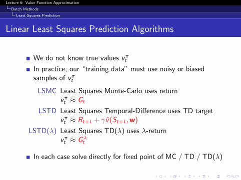
Linear Least Squares Prediction Algorithms
We do not know true values vπt
In practice, our “training data” must use noisy or biasedsamples of vπt
LSMC Least Squares Monte-Carlo uses returnvπt ≈ Gt
LSTD Least Squares Temporal-Difference uses TD targetvπt ≈ Rt+1 + γv̂(St+1,w)
LSTD(λ) Least Squares TD(λ) uses λ-returnvπt ≈ Gλ
t
In each case solve directly for fixed point of MC / TD / TD(λ)
Lecture 6: Value Function Approximation
Batch Methods
Least Squares Prediction
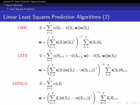
Linear Least Squares Prediction Algorithms (2)
LSMC 0 =T∑t=1
α(Gt − v̂(St ,w))x(St)
w =
(T∑t=1
x(St)x(St)>
)−1 T∑t=1
x(St)Gt
LSTD 0 =T∑t=1
α(Rt+1 + γv̂(St+1,w)− v̂(St ,w))x(St)
w =
(T∑t=1
x(St)(x(St)− γx(St+1))>
)−1 T∑t=1
x(St)Rt+1
LSTD(λ) 0 =T∑t=1
αδtEt
w =
(T∑t=1
Et(x(St)− γx(St+1))>
)−1 T∑t=1
EtRt+1

Lecture 6: Value Function Approximation
Batch Methods
Least Squares Prediction
Convergence of Linear Least Squares Prediction Algorithms
On/Off-Policy Algorithm Table Lookup Linear Non-Linear
On-Policy
MC 3 3 3
LSMC 3 3 -TD 3 3 7
LSTD 3 3 -
Off-PolicyMC 3 3 3
LSMC 3 3 -TD 3 7 7
LSTD 3 3 -

Lecture 6: Value Function Approximation
Batch Methods
Least Squares Control
Least Squares Policy Iteration
Starting w
π = greedy(q w)
qw = qπ
qw ≈ q*
Policy evaluation Policy evaluation by least squares Q-learning
Policy improvement Greedy policy improvement

Lecture 6: Value Function Approximation
Batch Methods
Least Squares Control
Least Squares Action-Value Function Approximation
Approximate action-value function qπ(s, a)
using linear combination of features x(s, a)
q̂(s, a,w) = x(s, a)>w ≈ qπ(s, a)
Minimise least squares error between q̂(s, a,w) and qπ(s, a)
from experience generated using policy π
consisting of 〈(state, action), value〉 pairs
D = {〈(s1, a1), vπ1 〉, 〈(s2, a2), vπ2 〉, ..., 〈(sT , aT ), vπT 〉}

Lecture 6: Value Function Approximation
Batch Methods
Least Squares Control
Least Squares Control
For policy evaluation, we want to efficiently use all experience
For control, we also want to improve the policy
This experience is generated from many policies
So to evaluate qπ(S ,A) we must learn off-policy
We use the same idea as Q-learning:
Use experience generated by old policySt ,At ,Rt+1,St+1 ∼ πoldConsider alternative successor action A′ = πnew (St+1)Update q̂(St ,At ,w) towards value of alternative actionRt+1 + γq̂(St+1,A
′,w))

Lecture 6: Value Function Approximation
Batch Methods
Least Squares Control
Least Squares Q-Learning
Consider the following linear Q-learning update
δ = Rt+1 + γq̂(St+1, π(St+1),w)− q̂(St ,At ,w)
∆w = αδx(St ,At)
LSTDQ algorithm: solve for total update = zero
0 =T∑t=1
α(Rt+1 + γq̂(St+1, π(St+1),w)− q̂(St ,At ,w))x(St ,At)
w =
(T∑t=1
x(St ,At)(x(St ,At)− γx(St+1, π(St+1)))>
)−1 T∑t=1
x(St ,At)Rt+1
Lecture 6: Value Function Approximation
Batch Methods
Least Squares Control
Least Squares Policy Iteration Algorithm
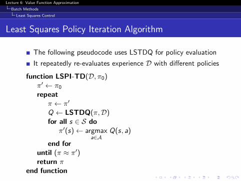
The following pseudocode uses LSTDQ for policy evaluation
It repeatedly re-evaluates experience D with different policies
function LSPI-TD(D, π0)π′ ← π0repeat
π ← π′
Q ← LSTDQ(π,D)for all s ∈ S do
π′(s)← argmaxa∈A
Q(s, a)
end foruntil (π ≈ π′)return π
end function
Lecture 6: Value Function Approximation
Batch Methods
Least Squares Control
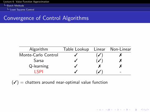
Convergence of Control Algorithms
Algorithm Table Lookup Linear Non-Linear
Monte-Carlo Control 3 (3) 7
Sarsa 3 (3) 7
Q-learning 3 7 7
LSPI 3 (3) -
(3) = chatters around near-optimal value function

Lecture 6: Value Function Approximation
Batch Methods
Least Squares Control
Chain Walk ExampleLeast-Squares Policy Iteration
1 2 3 4R R R
LLLL
R
0.9 0.9 0.9
0.9
0.90.90.9
0.9
0.1
0.1 0.1 0.1
0.1
0.10.10.1
r=0 r=1 r=1 r=0
Figure 9: The problematic MDP.
where s is the state number. LSPI was applied on the same problem using the same basisfunctions repeated for each of the two actions so that each action gets its own parameters:10
!(s, a) =
!
""""""#
I(a = L) ! 1I(a = L) ! sI(a = L) ! s2
I(a = R) ! 1I(a = R) ! sI(a = R) ! s2
$
%%%%%%&.
LSPI typically finds the optimal policy for this problem in 4 or 5 iterations. Samples foreach run were collected in advance by choosing actions uniformly at random for about 25(or more) steps and the same sample set was used throughout all LSPI iterations in the run.Figure 10 shows the iterations of one run of LSPI on a training set of 50 samples. Statesare shown on the horizontal axis and Q values on the vertical axis. The approximationsare shown with solid lines, whereas the exact values are connected with dashed lines. Thevalues for action L are marked with " and for action R with #. LSPI finds the optimalpolicy by the 2nd iteration, but it does not terminate until the 4th iteration, at which pointthe successive parameters (3rd and 4th iterations) are approximately equal. Notice thatthe approximations capture the qualitative structure of the value function, although thequantitative error is fairly big. The state visitation distribution for this training set was(0.24, 0.14, 0.28, 0.34). Although it was not perfectly uniform, it was “flat” enough toprevent an extremely uneven allocation of approximation errors over the state-action space.
LSPI was also tested on variants of the chain walk problem with more states and di!erentreward schemes to better understand and illustrate its behavior. Figure 11 shows a run ofLSPI on a 20-state chain with the same dynamics as above and a reward of +1 given onlyat the boundaries (states 1 and 20). The optimal policy in this case is to go left in states1–10 and right in states 11–20. LSPI converged to the optimal policy after 8 iterationsusing a single set of samples collected from a single episodes in which actions were chosenuniformly at random for 5000 steps. A polynomial of degree 4 was used for approximatingthe value function for each of the two actions, giving a block of 5 basis functions per action,
10. I is the indicator function: I(true) = 1 and I(false) = 0.
1131
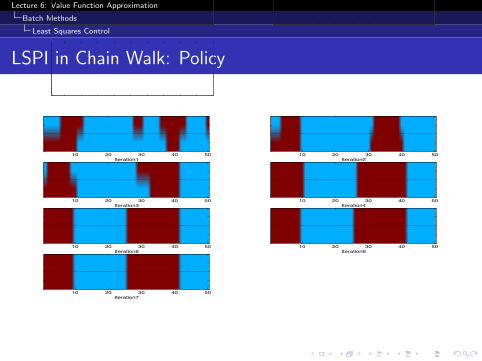
Consider the 50 state version of this problem
Reward +1 in states 10 and 41, 0 elsewhere
Optimal policy: R (1-9), L (10-25), R (26-41), L (42, 50)
Features: 10 evenly spaced Gaussians (σ = 4) for each action
Experience: 10,000 steps from random walk policy

Lecture 6: Value Function Approximation
Batch Methods
Least Squares Control
LSPI in Chain Walk: Action-Value FunctionLeast-Squares Policy Iteration
5 10 15 20 25 30 35 40 45 500
0.5
1
1.5
Iteration15 10 15 20 25 30 35 40 45 50
−0.50
0.51
1.5
Iteration2
5 10 15 20 25 30 35 40 45 500
2
4
Iteration35 10 15 20 25 30 35 40 45 50
0
2
4
Iteration4
5 10 15 20 25 30 35 40 45 500
2
4
Iteration55 10 15 20 25 30 35 40 45 50
0
2
4
Iteration6
5 10 15 20 25 30 35 40 45 500
2
4
Iteration7
Iteration110 20 30 40 50
Iteration210 20 30 40 50
Iteration310 20 30 40 50
Iteration410 20 30 40 50
Iteration510 20 30 40 50
Iteration610 20 30 40 50
Iteration710 20 30 40 50
Figure 13: LSPI iterations on a 50-state chain with a radial basis function approximator(reward only in states 10 and 41). Top: The state-action value function of thepolicy being evaluated in each iteration (LSPI approximation - solid lines; exactvalues - dotted lines). Bottom: The improved policy after each iteration (Raction - dark/red shade; L action - light/blue shade; LSPI - top stripe; exact -bottom stripe).
1135
Lecture 6: Value Function Approximation
Batch Methods
Least Squares Control
LSPI in Chain Walk: Policy
Least-Squares Policy Iteration
5 10 15 20 25 30 35 40 45 500
0.5
1
1.5
Iteration15 10 15 20 25 30 35 40 45 50
−0.50
0.51
1.5
Iteration2
5 10 15 20 25 30 35 40 45 500
2
4
Iteration35 10 15 20 25 30 35 40 45 50
0
2
4
Iteration4
5 10 15 20 25 30 35 40 45 500
2
4
Iteration55 10 15 20 25 30 35 40 45 50
0
2
4
Iteration6
5 10 15 20 25 30 35 40 45 500
2
4
Iteration7
Iteration110 20 30 40 50
Iteration210 20 30 40 50
Iteration310 20 30 40 50
Iteration410 20 30 40 50
Iteration510 20 30 40 50
Iteration610 20 30 40 50
Iteration710 20 30 40 50
Figure 13: LSPI iterations on a 50-state chain with a radial basis function approximator(reward only in states 10 and 41). Top: The state-action value function of thepolicy being evaluated in each iteration (LSPI approximation - solid lines; exactvalues - dotted lines). Bottom: The improved policy after each iteration (Raction - dark/red shade; L action - light/blue shade; LSPI - top stripe; exact -bottom stripe).
1135
Lecture 6: Value Function Approximation
Batch Methods
Least Squares Control
Questions?


