
Unit Root DF P-P Stationarity Tests Variance Ratio Structural Break UC
Lecture: Non-stationary Time Series
222061-1617: Time Series Econometrics
Spring 2021
Jacek Suda
222061-1617: Time Series Econometrics Lecture: Non-stationary Time Series

Unit Root DF P-P Stationarity Tests Variance Ratio Structural Break UC
Outline
Outline:
1 Unit Root
2 Structural Break
3 Unobserved Component Model and Trend/Cycle Decomposition
222061-1617: Time Series Econometrics Lecture: Non-stationary Time Series

Unit Root DF P-P Stationarity Tests Variance Ratio Structural Break UC Random Walk Statistical issues AR Tests
UNIT ROOT
222061-1617: Time Series Econometrics Lecture: Non-stationary Time Series
Unit Root DF P-P Stationarity Tests Variance Ratio Structural Break UC Random Walk Statistical issues AR Tests
Random Walk - Example
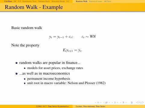
Basic random walk
yt = yt−1 + εt; εt ∼ WN
Note the propertyEtyt+1 = yt.
random walks are popular in finance...models for asset prices, exchange rates
...as well as in macroeconomicspermanent income hypothesisunit root in macro variable: Nelson and Plosser (1982)
222061-1617: Time Series Econometrics Lecture: Non-stationary Time Series
Unit Root DF P-P Stationarity Tests Variance Ratio Structural Break UC Random Walk Statistical issues AR Tests
Random Walk: Properties
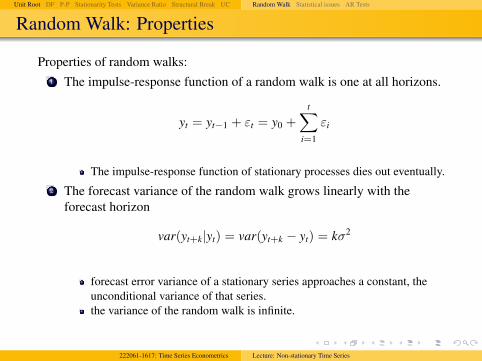
Properties of random walks:1 The impulse-response function of a random walk is one at all horizons.
yt = yt−1 + εt = y0 +
t∑i=1
εi
The impulse-response function of stationary processes dies out eventually.2 The forecast variance of the random walk grows linearly with the
forecast horizon
var(yt+k|yt) = var(yt+k − yt) = kσ2
forecast error variance of a stationary series approaches a constant, theunconditional variance of that series.the variance of the random walk is infinite.
222061-1617: Time Series Econometrics Lecture: Non-stationary Time Series
Unit Root DF P-P Stationarity Tests Variance Ratio Structural Break UC Random Walk Statistical issues AR Tests
Random Walk: Properties
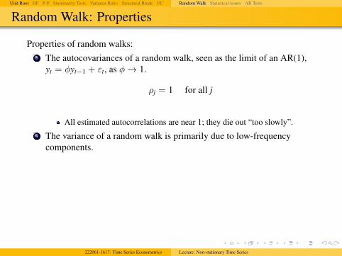
Properties of random walks:3 The autocovariances of a random walk, seen as the limit of an AR(1),
yt = φyt−1 + εt, as φ→ 1.
ρj = 1 for all j
All estimated autocorrelations are near 1; they die out “too slowly”.4 The variance of a random walk is primarily due to low-frequency
components.
222061-1617: Time Series Econometrics Lecture: Non-stationary Time Series
Unit Root DF P-P Stationarity Tests Variance Ratio Structural Break UC Random Walk Statistical issues AR Tests
Statistical issues: Distribution of AR(1) estimates
Recallyt = yt−1 + εt; εt ∼ WN
Dickey and Fuller:Test for a random walks by running yt = φyt−1 + εt and testing whetherφ = 1 not correct:
1 OLS estimates are biased down (towards stationarity)2 OLS standard errors are tighter than the actual standard errors
Many series thought to be stationary based on OLS regressions couldbe in fact generated by random walks.
222061-1617: Time Series Econometrics Lecture: Non-stationary Time Series
Unit Root DF P-P Stationarity Tests Variance Ratio Structural Break UC Random Walk Statistical issues AR Tests
Statistical issues: Inappropriate detrending
Suppose the real model is
yt = c + yt−1 + εt; εt ∼ WN
Suppose you detrend by OLS, and then estimate an AR(1), i.e., fit themodel
yt = α+ β · t + φyt−1 + εt
OLS estimate φ even more biased downward and standard errors moremisleading.
Why?In a relatively small sample, the random walk is likely to drift up ordown;Drift could well be (falsely) modeled by a linear (or nonlinear,“breaking” , etc. ) trend.
222061-1617: Time Series Econometrics Lecture: Non-stationary Time Series

Unit Root DF P-P Stationarity Tests Variance Ratio Structural Break UC Random Walk Statistical issues AR Tests
Statistical issues: Spurious regression
Suppose two series are generated by independent random walks,
xt = xt−1 + εt
yt = yt−1 + νt
E(εtνs) = 0 for all t, s
Suppose we run yt on xt by OLS,
yt = α+ βxt + υt
Assumptions behind the usual distribution theory are violated.We find statistically significant β more often than the we should.
222061-1617: Time Series Econometrics Lecture: Non-stationary Time Series

Unit Root DF P-P Stationarity Tests Variance Ratio Structural Break UC Random Walk Statistical issues AR Tests
Autoregressive Unit Root Tests
ARMA(p, q) process:
φ(L)yt = θ(L)εt, εt ∼ WN
Consider φ(z) = 0, where φ(z) is a characteristic equation.
φ(L) = 1− φ1L− φ2L2 − . . .− φpLp
φ(z) = 0⇒ 1− φ1z− φ2z2 − . . .− φpzp = 0
⇒ (1− 1λ1
z)(1− 1λ2
z) · · · (1− 1λp
z) = 0
H0 : φ(z) = 0 has (at least) one root on unit circle.
222061-1617: Time Series Econometrics Lecture: Non-stationary Time Series
Unit Root DF P-P Stationarity Tests Variance Ratio Structural Break UC Random Walk Statistical issues AR Tests
Unit Root in ARMA
If one of the roots is equal to one, it can be factored out
φ(z) = (1− z)φ∗(z),
⇒ φ∗(z) = 0 has roots outside unit circle
⇒ φ∗(L)(1− L)yt = φ(L)εt
∆yt = φ∗(L)−1θ(L)εt
∆yt = Ψ∗(L)εt
∆yt = ut, ut = Ψ∗(L)εt ∼ I(0)
n in I(n) denotes order of integration.I(0) denotes covariance stationary process.
222061-1617: Time Series Econometrics Lecture: Non-stationary Time Series

Unit Root DF P-P Stationarity Tests Variance Ratio Structural Break UC Random Walk Statistical issues AR Tests
Unit Root in ARMA
Thenyt = yt−1 + ut,
and, given y0,
yt = y0 +
t−1∑j=0
ut−j ∼ I(1).
Shocks do not die out.An alternative for H0 is
H1 : φ(z) = 0 has all roots outside unit circleyt = φ(L)−1θ(L)εt
yt = Ψ(L)εt = ut ∼ I(0)
Shocks will die out over time.
222061-1617: Time Series Econometrics Lecture: Non-stationary Time Series

Unit Root DF P-P Stationarity Tests Variance Ratio Structural Break UC Brownian Motion D-F 1 D-F 2 D-F 3 ADF
Brownian Motion
A Wiener process (Brownian motion) W(·) is a continuous-time stochasticprocess, associating each date r ∈ [0, 1] a scalar random variable W(r) thatsatisfies:
1 W(0) = 02 For any dates 0 ≤ t1 ≤ . . . ≤ tk ≤ 1, the changes
W(t2)−W(t1),W(t3)−W(t2), . . . ,W(tk)−W(tk−1) are independentnormal with
W(s)−W(t) ∼ N(0, (s− t))
3 W(s) is continuous in s.Intuition: A Wiener process is the scaled continuous time limit of a randomwalk.Properties:
W(r) ∼ N(0, r)
σW(r) ∼ N(0, σ2r)
W(r)2 ∼ rχ2(1)
222061-1617: Time Series Econometrics Lecture: Non-stationary Time Series
Unit Root DF P-P Stationarity Tests Variance Ratio Structural Break UC Brownian Motion D-F 1 D-F 2 D-F 3 ADF
Dickey-Fuller: Case 1
Consider AR(1):
yt = φyt−1 + εt, εt ∼ WN
φ(L) = 1− φL
Then
H0 : φ(z) = 0 has unit root ⇔ φ = 1H1 : φ(z) = 0 has roots outside unit circle ⇔ |φ| < 1
Standard test statistics:
tφ =φ− φSE(φ)
,
where φ comes from OLS on yt = φyt−1 + εt.
222061-1617: Time Series Econometrics Lecture: Non-stationary Time Series

Unit Root DF P-P Stationarity Tests Variance Ratio Structural Break UC Brownian Motion D-F 1 D-F 2 D-F 3 ADF
Dickey-Fuller Result
Testing for any φ 6= 1
tφ=0.9 =φ− 0.9
SE(φ)∼ t − distribution→ N(0, 1)
Testing for φ = 1:
tφ=1 =φ− 1
SE(φ)∼ DF
DF d−→∫ 1
0 W(r)dW(r)
(∫ 1
0 W(r)2dr)1/2
It is based on continuous time random walk processBoth numerator and denominator are functions of r,W
It is theoretical result: the distribution can be found numerically bysimulation
222061-1617: Time Series Econometrics Lecture: Non-stationary Time Series
Unit Root DF P-P Stationarity Tests Variance Ratio Structural Break UC Brownian Motion D-F 1 D-F 2 D-F 3 ADF
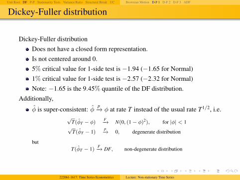
Dickey-Fuller distribution
Dickey-Fuller distributionDoes not have a closed form representation.Is not centered around 0.5% critical value for 1-side test is −1.94 (−1.65 for Normal)1% critical value for 1-side test is −2.57 (−2.32 for Normal)Note: −1.65 is the 9.45% quantile of the DF distribution.
Additionally,
φ is super-consistent: φp−→ φ at rate T instead of the usual rate T1/2, i.e.
√T(φT − φ)
F−→ N(0, (1− φ)2), for |φ| < 1√
T(φT − 1)p−→ 0, degenerate distribution
butT(φT − 1) F−→ DF, non-degenerate distribution
222061-1617: Time Series Econometrics Lecture: Non-stationary Time Series

Unit Root DF P-P Stationarity Tests Variance Ratio Structural Break UC Brownian Motion D-F 1 D-F 2 D-F 3 ADF
Superconsistency
Note that yt = ε1 + . . . εT ∼ N(0, σ2t)
φT =
∑Tt=1 yt−1yt∑Tt=1 y2
t−1
=⇒ φT − 1 =
∑Tt=1 yt−1εt∑T
t=1 y2t−1
, y0 = 0.
Since
y2t = (yt−1 + εt)
2 =⇒ yt−1εt =12(y2
t − y2t−1 − ε
2t ),
thenT∑
t=1
yt−1εt =12(y2
T − y20)−
12
T∑t=1
ε2t
Therefore, dividing the numerator by σ2T , we get
1σ2T
T∑t=1
yt−1εt =12
(yT
σ√
T
)2
−1
2σ2
1T
T∑t=1
ε2t
F−→12(X − 1)
where
X =
(yT
σ√
T
)2
∼ χ2(1),
1T
T∑t=1
ε2t
p−→ σ2
222061-1617: Time Series Econometrics Lecture: Non-stationary Time Series

Unit Root DF P-P Stationarity Tests Variance Ratio Structural Break UC Brownian Motion D-F 1 D-F 2 D-F 3 ADF
Superconsistency
Since yt−1 ∼ N(0, (t − 1)σ2), the mean of the denominator,∑T
t=1 y2t−1,
E
(T∑
t=1
y2t−1
)= σ2
T∑t=1
(t − 1) = σ2T(T − 1).
For∑T
t=1 y2t−1 to have convergent distribution, it has to be divided by T2.
Therefore,
T(φT − φ) =1T
∑Tt=1 yt−1εt
1T2
∑Tt=1 y2
t−1
to converge.
222061-1617: Time Series Econometrics Lecture: Non-stationary Time Series

Unit Root DF P-P Stationarity Tests Variance Ratio Structural Break UC Brownian Motion D-F 1 D-F 2 D-F 3 ADF
Nuisance parameter
Assumeyt = c + φyt−1 + εt
For H0 : φ = 0,
tφ=0 =φ− 0
SE(φ)
A∼ N(0, 1)
Asymptotically, the distribution is always N(0, 1), no matter what c andσ2 are.If the test statistics does not depend asymptotically on other parameters(nuisance parameter) it is pivotal.Note: It may not be pivotal for small sample; for example, for t = 100it may depend on c and/or σ2.
222061-1617: Time Series Econometrics Lecture: Non-stationary Time Series

Unit Root DF P-P Stationarity Tests Variance Ratio Structural Break UC Brownian Motion D-F 1 D-F 2 D-F 3 ADF
Nuisance parameter in DF
DF statistics, even asymptotically, depends on c: c is a nuisanceparameter.Dickey and Fuller shows that if φ = 1 nuisance parameters areimportant not only in small sample but also in asymptotic distribution(it’s no longer pivotal testing).The small-sample distribution for DF converges to asymptoticdistribution much faster than in normal case: even for t = 100 it willlook very much like asymptotical distribution; if φ = 0.9 it will requirea lot of observations to get to normal distribution.
222061-1617: Time Series Econometrics Lecture: Non-stationary Time Series
Unit Root DF P-P Stationarity Tests Variance Ratio Structural Break UC Brownian Motion D-F 1 D-F 2 D-F 3 ADF
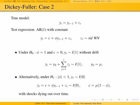
Dickey-Fuller: Case 2
True model:yt = yt−1 + εt
Test regression: AR(1) with constant
yt = c + φyt−1 + εt, εt ∼ iid WN
Under H0 : φ = 1 and c = 0, yt ∼ I(1) without drift
yt = y0 +
t∑j=1
εj ∼ I(1), y0 = µ,
Alternatively, under H1 : |φ| < 1, yt ∼ I(0)
yt = c + φyt−1 + εt ∼ I(0), c = µ(1− φ),
with shocks dying out over time.
222061-1617: Time Series Econometrics Lecture: Non-stationary Time Series

Unit Root DF P-P Stationarity Tests Variance Ratio Structural Break UC Brownian Motion D-F 1 D-F 2 D-F 3 ADF
Dickey-Fuller distribution
The t−statistics is
tµφ=1 =φ− 1
SE(φ)
from OLS regression yt = c + φyt−1 + εt,Dickey-Fuller shows that, under H0 : φ = 1, it is
tµφ=1d−→ DFµ =
∫ 10 Wµ(r)dW(r)
(∫ 1
0 Wµ(r)2dr)1/2,
with
Wµ(r) = W(r)−∫ 1
0W(r)dr
the “de-meaned” Wiener process,∫ 1
0 Wµ(r) = 0.
222061-1617: Time Series Econometrics Lecture: Non-stationary Time Series

Unit Root DF P-P Stationarity Tests Variance Ratio Structural Break UC Brownian Motion D-F 1 D-F 2 D-F 3 ADF
Remarks
If y0 = µ 6= 0, it converge to DFµ, if µ = 0 then DF, but it doesn’tmatter what value of y0 is.The asymptotic distributions of these test statistics are influenced by thepresence (but not the value) of the constant in the test regressionThe inclusion of a constant pushes the distributions of tµφ=1 to the left:
5% critical value for 1-side test is −2.86 (−1.65 for Normal)1% critical value for 1-side test is −3.43 (−2.32 for Normal)1.65 is the 45.94% quantile of the DFµ distribution!
222061-1617: Time Series Econometrics Lecture: Non-stationary Time Series

Unit Root DF P-P Stationarity Tests Variance Ratio Structural Break UC Brownian Motion D-F 1 D-F 2 D-F 3 ADF
Dickey-Fuller: Case 3
The test regression is
yt = c + β · t + φyt−1 + εt
and includes a constant and deterministic time trend to capture thedeterministic trend under the alternative.
222061-1617: Time Series Econometrics Lecture: Non-stationary Time Series

Unit Root DF P-P Stationarity Tests Variance Ratio Structural Break UC Brownian Motion D-F 1 D-F 2 D-F 3 ADF
Hypothesis
H0 : φ = 1, β = 0 : yt ∼ I(1) with drift
yt = y0 + c · t +
t∑j=1
εj ∼ I(1) with drift,
where y0 + c · t denotes deterministic component, and∑t
j=1 εj therandom walk component.H1 : |φ| < 1: yt ∼ I(0) with deterministic time trend
yt = c + β · t + φyt−1 + εt ∼ Trend stationaryyt − β · t ∼ I(0)
222061-1617: Time Series Econometrics Lecture: Non-stationary Time Series

Unit Root DF P-P Stationarity Tests Variance Ratio Structural Break UC Brownian Motion D-F 1 D-F 2 D-F 3 ADF
Test statistics
Test statistics
tβφ=1 =φ− 1
SE(φ)
where φ is from OLS regression
yt = c + β · t + φyt−1 + εt.
Both β and c are nuisance parameters.Under H0 : φ = 1
tβφ=1d−→ DFβ =
∫ 10 Wβ(r)dW(r)
(∫ 1
0 Wβ(r)2dr)1/2,
with
Wβ(r) = Wµ(r)− 12(
r − 12
)∫ 1
0
(s− 1
2
)W(s)ds,
222061-1617: Time Series Econometrics Lecture: Non-stationary Time Series

Unit Root DF P-P Stationarity Tests Variance Ratio Structural Break UC Brownian Motion D-F 1 D-F 2 D-F 3 ADF
Test statistics
De-meaned and detrended Wiener process.The inclusion of a constant and trend in the test regression further shiftsthe distribution of tβφ=1to the left.
5% critical value for 1-side test is −3.41 (−1.65 for Normal)1% critical value for 1-side test is −3.96 (−2.32 for Normal)1.65 is the 77.52% quantile of the DFβ distribution!
Test DFµ has more power than DFβ if β = 0.
222061-1617: Time Series Econometrics Lecture: Non-stationary Time Series

Unit Root DF P-P Stationarity Tests Variance Ratio Structural Break UC Brownian Motion D-F 1 D-F 2 D-F 3 ADF
Extending DF
The previous unit root tests are valid if the time series yt is wellcharacterized by an AR(1) with white noise errors.Many economic and financial time series have a more complicateddynamic structure than is captured by a simple AR(1) model.Said and Dickey (1984) augment the basic autoregressive unit root testto accommodate general ARMA(p, q) models with unknown orders andtheir test is referred to as the augmented Dickey-Fuller (ADF) test
222061-1617: Time Series Econometrics Lecture: Non-stationary Time Series

Unit Root DF P-P Stationarity Tests Variance Ratio Structural Break UC Brownian Motion D-F 1 D-F 2 D-F 3 ADF
Hypothesis
Basic AR(p) model
φ(L)yt = εt, εt ∼ WN
φ(L) = 1− φ1L− . . .− φpLp
Hypothesis
H0 : φ(z) = 0 has one unit rootφ(z) = (1− z)φ∗(z), φ∗(z) has no unit root.
H1 : φ(z) = 0 has all roots outside unit circle.
222061-1617: Time Series Econometrics Lecture: Non-stationary Time Series

Unit Root DF P-P Stationarity Tests Variance Ratio Structural Break UC Brownian Motion D-F 1 D-F 2 D-F 3 ADF
Transformation
Tranform φ(L)
yt = ρyt−1 + φ∗1∆yt−1 + φ∗2∆yt−2 + . . .+ φ∗p−1∆yt−p−1 + εt,
where
ρ = φ1 + φ2 + . . . φp
φ∗j = −p∑
k=j+1
φk
It’s just different representation of AR(p) process.Example: AR(2):
yt = φ1yt−1 + φ2yt−2 + εt
= φ1yt−1 + φ2yt−1 − φ2yt−1 + φ2yt−2 + εt
= (φ1 + φ2)yt−1 − φ2∆yt−1 + εt
= ρyt−1 + φ∗1∆yt−1 + εt.
222061-1617: Time Series Econometrics Lecture: Non-stationary Time Series

Unit Root DF P-P Stationarity Tests Variance Ratio Structural Break UC Brownian Motion D-F 1 D-F 2 D-F 3 ADF
Hypothesis restated
The hypothesis can be simply restated as
H0 : ρ = 1⇔ unit rootH1 : |ρ| < 1⇔ I(0)
in equationyt = ρyt−1 + ut, ut ∼ I(0)
with ut containing lagged differences to capture serial correlation in ut.
222061-1617: Time Series Econometrics Lecture: Non-stationary Time Series

Unit Root DF P-P Stationarity Tests Variance Ratio Structural Break UC Brownian Motion D-F 1 D-F 2 D-F 3 ADF
ADF
Augmented Dickey-Fuller Test (ADF Test)
tρ=1 =ρ− 1
SE(ρ)
from OLS regression
yt = ρyt−1 + φ∗1∆yt−1 + . . .+ φ∗p−1∆yt−p−1 + εt.
The distribution of t-statistics is
tρ=1d−→ DF
tµρ=1d−→ DFµ
tβρ=1d−→ DFβ .
222061-1617: Time Series Econometrics Lecture: Non-stationary Time Series

Unit Root DF P-P Stationarity Tests Variance Ratio Structural Break UC Brownian Motion D-F 1 D-F 2 D-F 3 ADF
Intuition
Re-parameterize AR(2) model
yt = ρyt−1 + φ∗1∆yt−1 + εt
ρ = φ1 + φ2
φ∗1 = −φ2
yt−1 ∼ I(1) ⇒ ρ has a non-normal, asymptotic “unit root”distribution;∆yt−1 ∼ I(0)⇒ φ∗1 has an asymptotic normal distribution
222061-1617: Time Series Econometrics Lecture: Non-stationary Time Series

Unit Root DF P-P Stationarity Tests Variance Ratio Structural Break UC Brownian Motion D-F 1 D-F 2 D-F 3 ADF
Remarks
Remarks:If φ(L)yt = θ(L)εt, ADF works asymptotically as p grows with samplesize at rate T1/3.If p unknown: choose large enough p to eliminate serial correlation inut in yt = ρyt−1 + ut.If p is too small then the remaining serial correlation in the errors willbias the test.If p is too large then the power of the test will suffer.Monte Carlo experiments suggest it is better to error on the side ofincluding too many lags.Choose max lag (e.g. 12 for monthly data). Test last lag with|tφ∗ | > 1.645Backward selection procedure.
222061-1617: Time Series Econometrics Lecture: Non-stationary Time Series

Unit Root DF P-P Stationarity Tests Variance Ratio Structural Break UC Statistics Phillips-Perron Unit-Root Test
Phillips-Perron Unit-Root Test
Model
∆yt = ρyt−1 + ut, ut– serially correlated residuals
We do not specify how it is correlated, do not put any parametricapproach.If∑φ∗ is close to −1, ADF has terrible size.
Phillips-Perron addresses this issue
222061-1617: Time Series Econometrics Lecture: Non-stationary Time Series

Unit Root DF P-P Stationarity Tests Variance Ratio Structural Break UC Statistics Phillips-Perron Unit-Root Test
Phillips-Perron Unit-Root Test
The PP tests correct for any serial correlation and heteroskedasticity inthe errors ut of the test regression.It directly modifies the test statistics tρ=0:
Zt =
(σ2
λ2
)1/2
tρ=0 −12
(λ2 − σ2
λ2
)(T · SE(ρ)
σ2
)
tρ=0 =ρ
SE(ρ)
222061-1617: Time Series Econometrics Lecture: Non-stationary Time Series

Unit Root DF P-P Stationarity Tests Variance Ratio Structural Break UC Statistics Phillips-Perron Unit-Root Test
Phillips-Perron Unit-Root Test
Terms σ2 and λ2 are consistent estimates of the variance parameters
σ2 = limT→∞
T−1T∑
t=1
E(u2t )
λ2 = limT→∞
T∑t=1
E(T−1S2T) = “long run variance”
ST =
T∑t=1
ut.
Result: Under the null hypothesis that ρ = 0, the PP Zt statistic has thesame asymptotic distributions as the ADF t-statistic.
222061-1617: Time Series Econometrics Lecture: Non-stationary Time Series

Unit Root DF P-P Stationarity Tests Variance Ratio Structural Break UC Statistics Phillips-Perron Unit-Root Test
Phillips-Perron Unit-Root Test
The sample variance of the least squares residual ut is a consistentestimate of σ2.The Newey-West long-run variance estimate of ut using ut is aconsistent estimate of λ2.
λ2 = γ0 + 2m∑
j=1
[1− j
m + 1
]γ∗j
γ0 =1T
T∑t=1
u2t
γ∗j =1T
T∑t=j+11
utut−j
222061-1617: Time Series Econometrics Lecture: Non-stationary Time Series

Unit Root DF P-P Stationarity Tests Variance Ratio Structural Break UC UC Model Unit MA root KPSS Test
Stationarity Tests
Nelson-Plosser found that most macro variables have unit roots.They failed to reject H0 of the presence of unit root (we may reject itbecause of the low power of the test).H0 in unit root test is that there is unit root and N-P fails to reject it.We want to reverse the problem and test if the series is stationary so thatunit root would make that we reject stationary H0.Kwiatkowski, Phillips, Schmidt and Shin (KPSS), 1992 JoE - nonparametric approach;Leybourne and McCabe (1994, JEBS) - parametric approach.
222061-1617: Time Series Econometrics Lecture: Non-stationary Time Series

Unit Root DF P-P Stationarity Tests Variance Ratio Structural Break UC UC Model Unit MA root KPSS Test
Unobserved Components Model
Unobserved Components Model
yt = µt + εt,
where
µt = µt−1 + ut ut ∼ iid(0, σ2u), µ0 = constant,
εt ∼ I(0) (i.e. φ(L)εt = θ(L)ηt)
µt is unobserved component.it takes both cases of unit root and stationarityµt = local mean + unobserved component: it changes every time.Even though we don’t observe this shock we can still recover it.
222061-1617: Time Series Econometrics Lecture: Non-stationary Time Series

Unit Root DF P-P Stationarity Tests Variance Ratio Structural Break UC UC Model Unit MA root KPSS Test
Stationarity Tests (KPSS)
Hypotheses:
H0 : σ2u = 0 =⇒ yt ∼ I(0)
H1 : σ2u > 0 =⇒ yt ∼ I(1)
Test is equivalent to testing for unit MA root in ∆yt.How to estimate variance σ2
u = 0, in model that is already difficult toestimate?
222061-1617: Time Series Econometrics Lecture: Non-stationary Time Series

Unit Root DF P-P Stationarity Tests Variance Ratio Structural Break UC UC Model Unit MA root KPSS Test
Unit MA root
So far we talked about AR unit root: σ2u > 0.
There is alternative approach MA unit root.
Unit MA root:
yt = µt + εt apply (1− L)
(1− L)yt = (1− L)µt + (1− L)εt
∆yt = ut + εt − εt−1
We never observe the shock (unless ut = 0).Under H0 : σ2
u = 0, ut = 0 so if there is a shock today then tomorrowwill exactly offset it => no accumulation of permanent shocks.So unit MA root implies no permanent effect of shock.
222061-1617: Time Series Econometrics Lecture: Non-stationary Time Series

Unit Root DF P-P Stationarity Tests Variance Ratio Structural Break UC UC Model Unit MA root KPSS Test
Granger representation
If εt ∼ iid, Granger representation theorem implies that
∆yt = et + θet−1,
where et is unobservable forecast error.If cov(ut, εt) = 0
cov(∆yt,∆yt−1) = cov(ut + εt − εt−1, ut−1 + εt−1 − εt−2) = −σ2ε
andcov(∆yt,∆yt−j) = 0, ∀j > 1
The same autocovariance structure as in MA(1) process.
222061-1617: Time Series Econometrics Lecture: Non-stationary Time Series

Unit Root DF P-P Stationarity Tests Variance Ratio Structural Break UC UC Model Unit MA root KPSS Test
Autocovariances
Compute autocovariances for both representationFor
∆yt = ut + εt − εt−1
the autocovariances are
γ0 = var(∆yt) = var(ut + εt − εt) = σ2u + 2σ2
ε
γ1 = cov(∆yt,∆yt−1) = −σ2ε
γj = 0, j > 1.
For∆yt = et + θet−1
the autocovariances are
γ∗0 = (1 + θ2)σ2e
γ∗1 = θσ2e
γ∗j = 0, j > 1.
222061-1617: Time Series Econometrics Lecture: Non-stationary Time Series

Unit Root DF P-P Stationarity Tests Variance Ratio Structural Break UC UC Model Unit MA root KPSS Test
Autocorrelations
Determine the mapping from UC-ARIMA parameters to reduced formARMA(0,1) model
Define q =σ2
uσ2ε
— signal-to-noise ratio1st-order autocorrelations:
ρ1 =γ1
γ0=−1
q + 2,
ρ∗1 =θ
1 + θ2
Set ρ1 = ρ∗1 and solve for θ
θ =−(q + 2)±
√(q + 2)2 − 4
2.
Note two values of θ consistent with original model.Choose the invertible solution, |θ| < 1.
222061-1617: Time Series Econometrics Lecture: Non-stationary Time Series

Unit Root DF P-P Stationarity Tests Variance Ratio Structural Break UC UC Model Unit MA root KPSS Test
MA(1) representation
∆yt = et + θet−1,
For σεu = 0
θ =−(q + 2) +
√q2 + 4q
2, q =
σ2u
σ2ε
.
q is the signal-to-noise ration.As q→ 0 we have unit MA root→ we have permanent shock but theyare very very small.If σ2
u = 0 then
q = 0 =⇒ θ =−22
= −1
so Ψ∗(L) = 1 + θL has unit root.
222061-1617: Time Series Econometrics Lecture: Non-stationary Time Series
Unit Root DF P-P Stationarity Tests Variance Ratio Structural Break UC UC Model Unit MA root KPSS Test
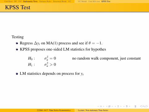
KPSS Test
TestingRegress ∆yt on MA(1) process and see if θ = −1.KPSS proposes one-sided LM statistics for hypothes
H0 : σ2u = 0 no random walk component, just constant
H1 : σ2u > 0
LM statistics depends on process for yt
222061-1617: Time Series Econometrics Lecture: Non-stationary Time Series

Unit Root DF P-P Stationarity Tests Variance Ratio Structural Break UC UC Model Unit MA root KPSS Test
KPSS: Case 1
Case 1: constant term only
yt = µt + εt
µt = µt−1 + ut, µ0 = constant
Test regressionyt = α+ εt =⇒ εt = yt − y
LM test:
ηµ =1
T2
T∑t=1
S2t
Λ2 ,
whereSt =
∑tj=1 εj is a partial sum over time of residuals, and
Λ2, spectral density at frequency 0
Sum up sample residual over time −→ under H0 they should not be abig number, they should cancel out. Otherwise, (under alternative) theyshould get larger and larger.
222061-1617: Time Series Econometrics Lecture: Non-stationary Time Series

Unit Root DF P-P Stationarity Tests Variance Ratio Structural Break UC UC Model Unit MA root KPSS Test
KPSS: Case 1
Under H0 : σ2u = 0
ηµd−→∫ 1
0V(r)2dr
where
V(r) = W(r)− rW(1) = standard Brownian Bridge
Reject at 5% if ηµ > 0.463.To do it need to estimate Λ2, spectral density at frequency 0.KPSS proposes against Bartlet kernel approach:
depending how you choose the bandwidth you get different statisticsdepending on what bandwidth you choose -> big sample size distortions.Some people suggest using parametric approach to construct test statistics.
222061-1617: Time Series Econometrics Lecture: Non-stationary Time Series

Unit Root DF P-P Stationarity Tests Variance Ratio Structural Break UC UC Model Unit MA root KPSS Test
KPSS: Case 2
Case 2: constant + trend
yt = τ · t + µt + εt, εt ∼ I(0)
µt = µt−1 + ut, ut ∼ iid(0, σ2u)
Test regressionyt = α+ τ · t + εt
LM test:
ηµ =1
T2
T∑t=1
S2t
Λ2 ,
Reject H0 at 5% if ητ > 0.146.
222061-1617: Time Series Econometrics Lecture: Non-stationary Time Series

Unit Root DF P-P Stationarity Tests Variance Ratio Structural Break UC UC Model Unit MA root KPSS Test
Testing
Now we have unit root and stationarity test: apply both.1 Unit root test: you can’t reject H0;
KPSS test: reject H0.Both imply that series has unit root.
2 If we can’t reject both test: data give not enough observations.3 Reject unit root, reject stationarity: both hypothesis are component
hypothesis – heteroskedasticity in series may make a big difference; ifthere is structural break it will affect inference.
Power problem: if there is small random walk component (smallvariance σ2
u), we can’t reject unit root and can’t reject stationarity.Economics: if the series is highly persistence we can’t reject H0 (unitroot) – highly persistent may be even without unit root but it also meanswe shouldn’t treat/take data in levels.If we want to quantify how important the unit root is, we should useVariance Ratio Test.
222061-1617: Time Series Econometrics Lecture: Non-stationary Time Series

Unit Root DF P-P Stationarity Tests Variance Ratio Structural Break UC Idea Variance Example Result
Variance ratio: Idea
Cochrane, 1988non-paramteric measure of “economic” importance of unit root
Idea
0 5 10 15 20 25 300
5
10
15
20
25
30
0 5 10 15 20 25 300
5
10
15
20
25
30
Variance of random walk grows linearly with horizon (no unconditionalvariance)Variance of trend stationary process is finite(it may grow over short horizon but it will finally settle down)
Test the behavior of variance.
222061-1617: Time Series Econometrics Lecture: Non-stationary Time Series

Unit Root DF P-P Stationarity Tests Variance Ratio Structural Break UC Idea Variance Example Result
Variance
LetVk = (1/k)var(Yt+k − Yt − kµ)
Vk the variance of kth period difference,µ is deterministic trend that does not affect the variance.
If there is no random walk it should converge to zero as variance isconverging to constant and k is growing.Rewrite it as
Vk =1k
E [(∆yt+1 − µ) + (∆yt+2 − µ) + . . .+ (∆yt+k − µ)]2
= γ∗0 + 2k−1∑j=1
(k − j
k
)γ∗j
= weighted average of auto-covariances γ∗j = cov(∆yt,∆yt+j)
Auto-covariances are important because everything about thecovariance-stationary series is in auto-covariance generating function.If model reduced to covariances, we can do analysis non-parametrically– just use sample auto-covariances.
222061-1617: Time Series Econometrics Lecture: Non-stationary Time Series

Unit Root DF P-P Stationarity Tests Variance Ratio Structural Break UC Idea Variance Example Result
Variance ratio
Compute variance ratio
VRk =Vk
V1, V1 = γ∗0
Result
limk→∞
Vk =
∞∑k=−∞
γ∗k = Λ2
(spectral density at frequency 0 for ∆y)
222061-1617: Time Series Econometrics Lecture: Non-stationary Time Series

Unit Root DF P-P Stationarity Tests Variance Ratio Structural Break UC Idea Variance Example Result
Example: Random Walk
Random walk
yt = yt−1 + εt, εt ∼ N(0, σ2ε)
Then
yt = y0 +
t∑j=1
εj, yt+k = y0 +
t+k∑j=1
εj
yt+k − yt =
t+k∑j=t+1
εj
Variance
var(yt+1 − yt) = σ2ε, var(yt+k − yt) = kσ2
ε
V1 = σ2ε; Vk =
1k
var(yt+k − yt) = σ2ε ∀k
Variance ratio:
VRk =Vk
V1=σ2ε
σ2ε
= 1, ∀k.
shock today has effect on series today and on series in the future.222061-1617: Time Series Econometrics Lecture: Non-stationary Time Series

Unit Root DF P-P Stationarity Tests Variance Ratio Structural Break UC Idea Variance Example Result
Example: White Noise
White noiseyt = εt, εt ∼ N(0, σ2
ε)
Variance
var(yt+1 − yt) = 2σ2ε
var(yt+k − yt) = 2σ2ε
Vk =2σ2
ε
k∀k
Variance ratioVRk =
1k→ 0 as k→∞
So for different type of process the variance ratio behaves differently.In practice, we have to estimate VRk.Cochrane estimates VRk using Newey-West Λ2
NW , γ∗0 , γ∗j .
222061-1617: Time Series Econometrics Lecture: Non-stationary Time Series

Unit Root DF P-P Stationarity Tests Variance Ratio Structural Break UC Idea Variance Example Result
Implications
1 If VRk → 1
1k0
1
VRk
random walk, all shocks are permanent
2 If VRk → 0
1k0
1
VRk
trend stationary I(0) process
222061-1617: Time Series Econometrics Lecture: Non-stationary Time Series

Unit Root DF P-P Stationarity Tests Variance Ratio Structural Break UC Idea Variance Example Result
Implications
If k too large you get spurious “mean reversion”.In sample it always the case that
γ0 +
T−1∑h=1
γ∗h = 0
so mean reversion has to appear.Which k to use? : balance the two effects.Non parametric approach makes problem in small sample.At long horizon GDP has neither VR→ 0 not VR→ 1, it’s between.With standard errors, though, you can’t reject any of them.
222061-1617: Time Series Econometrics Lecture: Non-stationary Time Series

Unit Root DF P-P Stationarity Tests Variance Ratio Structural Break UC Structural Breaks Trend Test statistics Perron (1989) Criticism
STRUCTURAL BREAK
222061-1617: Time Series Econometrics Lecture: Non-stationary Time Series
Unit Root DF P-P Stationarity Tests Variance Ratio Structural Break UC Structural Breaks Trend Test statistics Perron (1989) Criticism
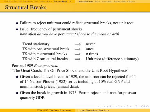
Structural Breaks
Failure to reject unit root could reflect structural breaks, not unit rootIssue: frequency of permanent shockshow often do you have permanent shock to the mean or drift
Trend stationary =⇒ neverTS with one structural break =⇒ onceTS with n structural breaks =⇒ n timesTS with T structural breaks =⇒ Unit root (difference stationary)
Perron, 1989 Econometrica,“The Great Crash, The Oil Price Shock, and the Unit Root Hypothesis”
Given a level a level break in 1929, the unit root can be rejected for 11of 14 Nelson-Plosser (1982) series including at 10% real GNP andnominal stock prices. (annual data).Given the break in growth in 1973, Perron rejects unit root for postwarquarterly GDP.
222061-1617: Time Series Econometrics Lecture: Non-stationary Time Series
Unit Root DF P-P Stationarity Tests Variance Ratio Structural Break UC Structural Breaks Trend Test statistics Perron (1989) Criticism
Model A: The “Great Crash” Model
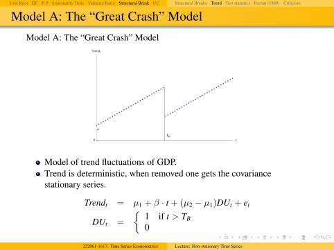
Model A: The “Great Crash” Model
TB
m
t0
Trendt
Model of trend fluctuations of GDP.Trend is deterministic, when removed one gets the covariancestationary series.
Trendt = µ1 + β · t + (µ2 − µ1)DUt + et
DUt =
{1 if t > TB
0
222061-1617: Time Series Econometrics Lecture: Non-stationary Time Series

Unit Root DF P-P Stationarity Tests Variance Ratio Structural Break UC Structural Breaks Trend Test statistics Perron (1989) Criticism
Model B: The “Oil Shock” Model
Model B: The “Oil Shock” Model
TB
m
Slope b1
Slope b2
t0
Trendt
Trendt = µ+ β1 · t + (β2 − β1)DT∗t + et
DT∗t =
{t − TB if t > TB
0
222061-1617: Time Series Econometrics Lecture: Non-stationary Time Series

Unit Root DF P-P Stationarity Tests Variance Ratio Structural Break UC Structural Breaks Trend Test statistics Perron (1989) Criticism
Model C: The “Combo” Model
Model C: The “Combo” Model
TB
Slope b2
Slope b1
m1
t0
Trendt
Trendt = µ1 + β1 · t + (µ2 − µ1)DUt + (β2 − β1)DT∗t + et
DUt =
{1 if t > TB
0
DT∗t =
{t − TB if t > TB
0
Model of nominal stock prices222061-1617: Time Series Econometrics Lecture: Non-stationary Time Series

Unit Root DF P-P Stationarity Tests Variance Ratio Structural Break UC Structural Breaks Trend Test statistics Perron (1989) Criticism
Test statistics
Maybe there is more structural breaks but only one big.Perron: do unit root test as always, OLS:
yt = ρyt−1 + Trendt(λ) +
p−1∑k=1
φ∗k ∆yt−k + εt
λ = TBT denotes location of break date.
Lagged difference to capture serial correlation.The t-statistics
tρ=1(λ) =ρ(λ)− 1
SE(ρ(λ))
We have more nuisance parameters that affect distribution
tρ=1(λ)A∼∫ 1
0 Wλ(r)dWλ(r)(∫ 10 Wλ(r)2dr
)1/2 ,
Wλ is demeaned, detrended, dedummied Brownian motion.The distribution is shifted further left than ADF.
222061-1617: Time Series Econometrics Lecture: Non-stationary Time Series

Unit Root DF P-P Stationarity Tests Variance Ratio Structural Break UC Structural Breaks Trend Test statistics Perron (1989) Criticism
Perron (1989)
222061-1617: Time Series Econometrics Lecture: Non-stationary Time Series

Unit Root DF P-P Stationarity Tests Variance Ratio Structural Break UC Structural Breaks Trend Test statistics Perron (1989) Criticism
Perron (1989)
222061-1617: Time Series Econometrics Lecture: Non-stationary Time Series

Unit Root DF P-P Stationarity Tests Variance Ratio Structural Break UC Structural Breaks Trend Test statistics Perron (1989) Criticism
Perron (1989)
222061-1617: Time Series Econometrics Lecture: Non-stationary Time Series

Unit Root DF P-P Stationarity Tests Variance Ratio Structural Break UC Structural Breaks Trend Test statistics Perron (1989) Criticism
Criticism
Data mining: How did Perron know the structural break was in 1929?He looked into data.λ must be chosen independently of the data for the correct size of thetest (or else there is bias against unit root, Zivot and Andrews, 1992JBES)
size: if H0 true how often you reject itpower: if H1 is true (H0 false) how often do you rejectSmall size and large power is optimal. We normally fix size (e.g.5% sizeand make test as powerful as possible.
t5% = −3.8 critical valueλ chosen after looking at data: choosing λ so that it generates thelargest t-statistics–test distributions is ever ore shifted so actual sizemight be bigger. Actual size might be 30% even though was set to 5%.
222061-1617: Time Series Econometrics Lecture: Non-stationary Time Series

Unit Root DF P-P Stationarity Tests Variance Ratio Structural Break UC Structural Breaks Trend Test statistics Perron (1989) Criticism
Criticism: Zivot and Andrews, 1992
Need a model of break date selection procedure (Zivot and Andrews,1992)λINF = break dates that produces the largest value of |tρ=1(λ)| over allλs in the sample.
tρ=1(λINF) = infλ∈Λ{tρ=1(λ)}
Zivot and Andrews find that for 8 of 14 Nelson-Plosser series (includingGNP) λINF = 1929 are stationary and the t-statistics is distributed as
tρ=1(λINF)A∼ infλ∈Λ
∫ 1
0 Wλ(r)d Wλ(r)(∫ 10 Wλ(r)2dr
)1/2
.
It shifts distribution further left of Perron’s.
222061-1617: Time Series Econometrics Lecture: Non-stationary Time Series

Unit Root DF P-P Stationarity Tests Variance Ratio Structural Break UC Detrending Trend/Cycle Example Estimation State-Space MNZ
UNOBSERVED COMPONENT
MODEL
222061-1617: Time Series Econometrics Lecture: Non-stationary Time Series
Unit Root DF P-P Stationarity Tests Variance Ratio Structural Break UC Detrending Trend/Cycle Example Estimation State-Space MNZ
Detrending
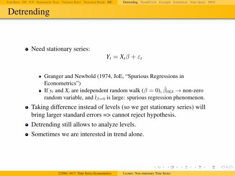
Need stationary series:Yt = Xtβ + εt
Granger and Newbold (1974, JoE, “Spurious Regressions inEconometrics”)If yt and Xt are independent random walk (β = 0), βOLS → non-zerorandom variable, and tβ=0 is large: spurious regression phenomenon.
Taking difference instead of levels (so we get stationary series) willbring larger standard errors => cannot reject hypothesis.Detrending still allows to analyze levels.Sometimes we are interested in trend alone.
222061-1617: Time Series Econometrics Lecture: Non-stationary Time Series
Unit Root DF P-P Stationarity Tests Variance Ratio Structural Break UC Detrending Trend/Cycle Example Estimation State-Space MNZ
Trend/Cycle
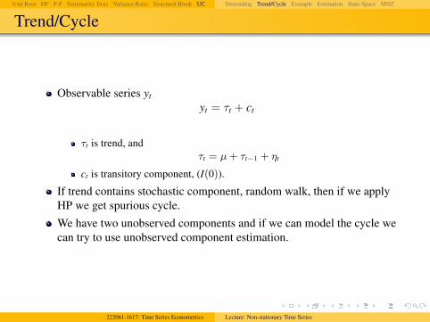
Observable series yt
yt = τt + ct
τt is trend, andτt = µ+ τt−1 + ηt
ct is transitory component, (I(0)).
If trend contains stochastic component, random walk, then if we applyHP we get spurious cycle.We have two unobserved components and if we can model the cycle wecan try to use unobserved component estimation.
222061-1617: Time Series Econometrics Lecture: Non-stationary Time Series

Unit Root DF P-P Stationarity Tests Variance Ratio Structural Break UC Detrending Trend/Cycle Example Estimation State-Space MNZ
Unobserved Components Approach
Watson (1986, JME), Clark (1987, QJE), Morley, Nelson, Zivot (2003,ReStat)Approach: parametric model for ct
Model (“Structural")
yt = τt + ct
τt = µ+ τt−1 + ηt, ηt ∼ iidN(0, σ2η)
φ(L)ct = εt, εt ∼ iidN(0, σ2ε),
cov(ηt, εt) = σεη
222061-1617: Time Series Econometrics Lecture: Non-stationary Time Series

Unit Root DF P-P Stationarity Tests Variance Ratio Structural Break UC Detrending Trend/Cycle Example Estimation State-Space MNZ
Problem: Identification
We have 1 observable series and 2 unobservable components.To get 2 unobservable components, we need some identificationassumptions.
Identification:If ct = εt or ct = φct−1 + εt, then σεη is not identified from the data.There can be infinitely many values of σεη that would produce the sameautocovariance generating function for the first series.However, that does not mean that all values of σεη are equal.If it is set to zero, it imposes restriction on autocovariance generatingfunction of 1st differences.
222061-1617: Time Series Econometrics Lecture: Non-stationary Time Series

Unit Root DF P-P Stationarity Tests Variance Ratio Structural Break UC Detrending Trend/Cycle Example Estimation State-Space MNZ
Example: AR(1)
Example: AR(1)
yt = τt + ct
τt = µ+ τt−1 + ηt
ct = φct−1 + εt
Structural model: 5 parameters: µ, σ2η, σ
2ε, φ, σεη .
How many parameters can be identified from data?Reduced-Form
First-difference equation
yt = τt + ct
(1− L)yt = (1− L)τt + (1− L)ct
∆yt = µ+ ηt + (1− L)(1− φL)−1εt
222061-1617: Time Series Econometrics Lecture: Non-stationary Time Series

Unit Root DF P-P Stationarity Tests Variance Ratio Structural Break UC Detrending Trend/Cycle Example Estimation State-Space MNZ
Example: AR(1)
Multiply both sides by (1− φL):
(1− φL)∆yt = (1− φL)µ+ (1− φL)ηt + (1− L)εt
= c + ηt − φηt−1 + εt − εt−1, c = (1− φ)µ.
They are unobserved but we have a sum of two iid series
ηt + εt + (−φ)ηt−1 + (−1)εt−1
The sum of two white noise processes = white noise: same moments asMA(1).So this model is observationally equivalent to
∆yt = c + φ∆yt−1 + et + θet−1
ARMA(1,1) =⇒ 4 parameters: c, φ, θ, σ2e , that’s how many we can
estimate.We have 5 parameters but only 4 observed. So far estimates assumesone of parameters fixed.
222061-1617: Time Series Econometrics Lecture: Non-stationary Time Series

Unit Root DF P-P Stationarity Tests Variance Ratio Structural Break UC Detrending Trend/Cycle Example Estimation State-Space MNZ
Estimation
Assume σεη = 0 (Watson, Harvey, Clark).=> shocks that drive transitory movements are not correlated with thosethat drive long-run behavior.With this assumption the model can be estimated:
1 Find match (functional) of observed/estimated parameters with the onesfrom structural model, or
2 Cast the model in a state space form and estimate via Kalman Filter:
222061-1617: Time Series Econometrics Lecture: Non-stationary Time Series

Unit Root DF P-P Stationarity Tests Variance Ratio Structural Break UC Detrending Trend/Cycle Example Estimation State-Space MNZ
State-Space Form
Observation equation
yt =[
1 1] [ τt
ct
]yt = Hβt
State equation[τt
ct
]=
[µ0
]+
[1 00 φ
] [τt−1ct−1
]+
[ηt
εt
],
βt = µ+ Fβt−1 + et, et ∼ N(0,Q),
Q =
[σ2η 0
0 σ2ε
]
222061-1617: Time Series Econometrics Lecture: Non-stationary Time Series

Unit Root DF P-P Stationarity Tests Variance Ratio Structural Break UC Detrending Trend/Cycle Example Estimation State-Space MNZ
Kalman Filter: Results
Kalman Filter does not care about how we came up with state form.KF: τt|t and ct|t, τt|T , ct|T .We say τt and ct are uncorrelated with each other, by assumption.corr(ηt|t, εt|t) = −1 even though we assume corr(ηt, εt) = 0.In classical approach corr(xt, εt) = 0 by construction, even though truerelationship is corr(xt, εt) 6= 0.Estimates of correlation rather than sample correlation of estimates.Identification: If we estimate the model without assuming σεη Gausswill not converge as there is∞ many numbers of σεη for whichlikelihood doesn’t decrease.
222061-1617: Time Series Econometrics Lecture: Non-stationary Time Series

Unit Root DF P-P Stationarity Tests Variance Ratio Structural Break UC Detrending Trend/Cycle Example Estimation State-Space MNZ
Morley, Nelson and Zivot (2003)
RW + AR(2) makes model identified.
Why?AR(1) cycles is not observationally different from RW.AR(2) has this feature that cannot be proxied by RW.
Morley, Nelson and Zivot (2003):σεη identified for ct ∼ ARMA(p, q), with p ≥ q + 2.
222061-1617: Time Series Econometrics Lecture: Non-stationary Time Series

Unit Root DF P-P Stationarity Tests Variance Ratio Structural Break UC Detrending Trend/Cycle Example Estimation State-Space MNZ
Example: AR(2)
Model:
yt = τt + ct
τt = µ+ τt−1 + ηt
ct = φ1ct−1 + φ2ct−2 + εt
6 parameters: µ, φ1, φ2, σ2η, σ
2ε, σεη .
Pre-multiplying both sides with (1− L):
∆yt = (1− L)τt + (1− L)ct
= µ+ ηt + (1− L)(1− φ1L− φ2L2)−1εt
(1− φ1L− φ2L2)∆yt = (1− φ1 − φ2)µ+ ηt − φ1ηt−1 − φ2ηt−2 + εt − εt−1
The model is observationally equivalent to ARMA(2,2) model:∆yt ∼ ARMA(2, 2) with 6 parameters: c, φ1, φ2, θ1, θ2, σ
2e .
222061-1617: Time Series Econometrics Lecture: Non-stationary Time Series

Unit Root DF P-P Stationarity Tests Variance Ratio Structural Break UC Detrending Trend/Cycle Example Estimation State-Space MNZ
Results
We can map parameters of ARMA(2,2) to our structural model orestimate KF with.
Q =
[σ2η σεη
σεη σ2ε
]For US real GDP, setting σεη = 0 can be rejected: ρεη = −0.9 .τt is volatileStructural model with AR(3) has 7 structural parameters but isobservationally equivalent to reduced-form version ARMA(3,3) with 8parameters: overidentification.Not such a big problem; ρεη < 0 still holds.
222061-1617: Time Series Econometrics Lecture: Non-stationary Time Series


