
Lecture Notes 2004
Sergiu Klainerman
Department of Mathematics, Princeton University, Princeton NJ 08544
E-mail address: [email protected]

CHAPTER 1
Basic Tools of Analysis
1. Distribution Theory
This is a very short summary of distribution theory, for more exposure to thesubject I suggest F.G. Friedlander and M. Joshi’s excellent book “ Introductionto the theory of distributions” in Cambridge university press. Hormander’s firstvolume of “ the analysis of linear PDE” in Springer can also be useful.
Notation. Throughout these notes we use the notation A . B to mean a ≤ cBwhere c is a numerical constant, independent of A,B.
1.1. Test Functions. Distributions. We start with some standard nota-tion. We denote vectors in Rn by x = (x1, . . . , xn) and set λx = (λx1, . . . , λxn),x+ y = (x1 + y1, . . . , xn + yn). We denote by x · y the standard scalar product andby |x| = (x · x) 1
2 the Euclidean length of x. Given a function f : Ω → C we denoteby supp(f) the closure in Ω of the set where f(x) 6= 0. We denote by Ck(Ω) the setof complex valued functions on Ω which are k times continuously differentiable andby Ck0 (Ω) the subset of those which are also compactly supported. We also denoteby C∞(Ω) = ∩k∈NCk(Ω) the space of infinitely differentiable functions; C∞0 (Ω) thesubset of those which also have compact support. The latter plays a particularlyimportant role in the theory of distributions; it is called the space of test functionson Ω.
Let Ω ⊂ Rn and f ∈ C∞(Ω). We denote by ∂if the partial derivative ∂f∂xi
, i =1, . . . , n. For derivatives of higher order we use the standard multi-index notation.A multi-index α is an n-tuple α = (α1, . . . , αn) of nonnegative integers with length|α| = α1+· · ·+αn. Set α+β = (α1+β1, . . . , αn+βn). We denote by α! the productof factorials α1! · · ·αn!. Now set ∂αf = ∂α1
1 · · · ∂αnn f . Clearly ∂α+βf = ∂α∂βf .
Given two smooth functions u, v we have the Leibnitz formula,
∂α(u · v) =∑
β+γ=α
α!β!γ!
∂βu∂γv.
Taylor’s formula, around the origin, for a smooth function f : Rn → C can bewritten as follows,
f(x) =∑|α|≤k
1α!∂αf(0)xα +O(|x|k+1) as x→ 0.
Here xα denotes the monomial xα = xα11 · · ·xαn
n .
3
4 1. BASIC TOOLS OF ANALYSIS
Proposition 1.2. Let f ∈ Ck0 (Rn), 0 ≤ k < ∞. Let ρ be a test function, i.e.ρ ∈ C∞0 (Rn) with supp(ρ) ⊂ B(0, 1), the ball centered at the origin of radius 1, and∫ρ(x)dx = 1. We set ρε(x) = ε−nρ(x/ε) and let
fε(x) = f∗ρε(x) = ε−n∫f(y)ρ(
x− y
ε)dy =
∫f(x− εz)ρ(z)dz.
We have:
(1) The functions fε are in C∞0 (Rn) and supp(f) ⊂ supp(f) +B(0, ε).(2) We have ∂αfε−→∂αf uniformly as ε→ 0.
Proof : The first part of the proposition follows immediately from the definitionsince the statement about supports is immediate and, by integration by parts, wecan transfer all derivatives of fε on the smooth part of the integrand ρε. To provethe second statement we simply write,
∂αfε(x)− ∂αf(x) =∫ (
∂αf(x− εz)− ∂αf(x))ρ(z)dz.
Therefore, for |α| ≤ k,
|∂αfε(x)− ∂αf(x)| ≤∫|∂αf(x− εz)− ∂αf(x)|ρ(z)|dz
≤∫|ρ(z)|dz sup
|y|≤ε|∂αf(x− εz)− ∂αf(x)|
. sup|y|≤ε
|∂αf(x− εz)− ∂αf(x)|
The proof follows now easily in view of the uniform continuity of the functions ∂αf .
As a corollary of the Proposition one can easily check that the space of test functionsC∞0 (Ω) is dense in the spaces Ck(Ω) as well as Lp(Ω), 1 ≤ p <∞.
Definition 1.3. A distribution u ∈ D′(Ω) is a linear functional u : C∞0 (Ω) → Cverifying the following property:
For any compact set K ⊂ Ω there exists an integer N and a constant C = CK,Nsuch that for all φ ∈ C∞0 (Ω), with supp(φ) ⊂ K we have
| < u, φ > | ≤ C∑|α|≤N
sup |∂αφ|.
Equivalently a distribution u is a linear functional u : C∞0 (Ω) → C which is con-tinuous if the space of test functions is endowed with the standard Frechet spacestructure1. In this topology a sequence φj converges to 0 in C∞0 (Ω) if all the sup-ports of φj are included in a compact subset of Ω and, for each multi-index α,
1This is the topology induced by the countable family of seminorms φ 7→ supKi|∂(α)φ|, where
Ki is a countable family of compact sets exhausting Ω, and α ranges over all natural multi-indices.
We do not need however the precise definition.
1. DISTRIBUTION THEORY 5
∂αφj → 0 in the uniform norm. We have in fact the following characterization ofdistributions:
Proposition 1.4. A linear form u : C∞0 (Ω) −→ C is a distribution in D′(Ω) ifflimj→∞ u(φj) = 0 for every sequence of test functions φj which converges to 0, inC∞0 (Ω), as j →∞.
Example 1: Any locally integrable function f ∈ L1loc(Ω) defines a distribution,
< f, φ >=∫fφ, ∀φ ∈ C∞0 (Ω).
We can thus identify L1loc(Ω) as a subspace of D′(Ω). This is true in particular for
the space C∞(Ω) ⊂ L1loc(Ω).
Example 2: The Dirac measure with mass 1 supported at x0 ∈ Rn is definedby,
< δx0 , φ >= φ(x0).
Remark: We shall often denote the action of a distribution u on a test functionby u(φ) instead of < u, φ >. Thus δx0(φ) = φ(x0).
Definition 1.5. A sequence of distributions uj ∈ D′(Ω) is said to converge, weakly,to a distribution u ∈ D′(Ω) if, uj(φ) → u(φ) for all φ ∈ C∞0 (Ω).
For example the sequence um = eimx converges weakly to 0 in D′(R) as m → ∞.Also if f ∈ L1(Rn), with
∫Rn f(x)dx = 1, the family of functions fλ(x) = λnf(λx)
converges weakly to δ0 as λ→∞.
1.6. Operations with distributions. The advantage of working with thespace of distributions is that while this space is much larger than the space ofsmooth functions most important operations on test functions can be carried overto distributions.
1. Multiplication with smooth functions: Given u ∈ D′(Ω) and f ∈ C∞(Ω)we define,
< fu, φ >=< u, fφ >, ∀φ ∈ C∞0 (Ω).
It is easily verified that multiplication with a smooth function is a continuousendomorphism of the space of distributions.
2. Convolution with a test-function: Consider, u ∈ D′(Rn), φ ∈ C∞0 (Rn).Generalizing the convolution of 2 functions in a natural way, we define
u∗φ(x) =< uy, φ(x− y) >,
the subscript specifying that u is understood to be acting on functions of the variabley. Observe that the definition coincides, indeed, with the usual one if u is a locallyintegrable function, u ∈ L1
loc(Rn).
6 1. BASIC TOOLS OF ANALYSIS
Remark: Observe that for every distribution u ∈ D′(Rn) and φ ∈ C∞0 (Rn) wehave u∗φ ∈ C∞(Rn). Indeed, e.g. letting ek denote a standard unit vector,
u∗φ(x+ hek)− u∗φ(x)h
= h−1 < uy, φ(x+ hek − y)− φ(x− y) >
= < uy,
∫ 1
0
∂kφ(x+ thek − y)dt > .
Now if x ∈ K, for some compact set K ⊂ Rn, then for every sequence hi → 0,the associated sequence of functions y 7→
∫ 1
0∂kφ(x + thiek − y)dt, together with
all its derivatives, converge uniformly toward ∂kφ(x − y) and its correspondingderivatives. Moreover they are all compactly supported with supports contained insome compact set K ′. Therefore,
limh→0
u∗φ(x+ hek)− u∗φ(x)h
= u∗∂kφ(x).
and thus u∗φ has continuous partial derivatives. We can continue in this mannerand conclude that in fact u∗φ ∈ C∞(Rn).
3. Differentiation of distributions: For every distribution u ∈ D′(Ω) we define
< ∂αu, φ >= (−1)|α| < u, ∂αφ > .
Again, it is easily verified that we have thus defined a continuous endomorphismof the space of distributions. Of course, the operations above were defined so as toextend the usual operations on smooth functions.
We can now define the action of a general linear partial differential operator ondistributions. Indeed let,
P (x, ∂) =∑|α|≤m
aα∂α, aα ∈ C∞(Ω),
be such an operator. Then,
< P (x, ∂)u, φ >=< u,P (x, ∂)†φ >,
where P (x, ∂)† is the formal adjoint operator,
P (x, ∂)†v =∑|α|≤m
(−1)|α|∂α(aαv).
Observe that if uj ∈ D′(Ω) converges weakly to u ∈ D′(Ω) then P (x, ∂)uj convergesweakly to P (x, ∂)u.
Exercise. Show that for all u ∈ D′(Ω) there exists a sequence uj ∈ C∞0 (Ω) suchthat uj → u as j → ∞ in the sense of distributions( weak convergence). ThusC∞0 (X) is dense in D′(Ω), with respect to the weak topology of the latter.
1.7. Example of distributions on the real line.
1.) The simplest nontrivial distribution is the Dirac function δ0 = δ0(x), definedby < δ0(x), φ >= φ(0).
1. DISTRIBUTION THEORY 7
2.) Another simple example is the Heavyside function H(x) equal to 1 for x > 0and zero for x ≤ 0. Or, using the standard identification between locally integrablefunctions and distributions,
< H(x), φ >=∫ ∞
0
φ(x)dx.
Observe that H ′(x) = δ0(x).3.) A more elaborate example is pv( 1
x ), or simply 1x , called the principal value
distribution,
<1x, φ >= lim
ε→0
( ∫ −ε
−∞
1xφ(x)dx+
∫ ∞
ε
1xφ(x)dx
).
Observe that log |x| is locally integrable and thus distribution by the standard iden-tification. It is easy to check that d
dx log |x| = pv( 1x ).
Exercise. Let, for z ∈ C with 0 < arg(z) < π, log z = log |z|+ iarg(z). We canregard x → log z = log(x + iy) as a family of distributions depending on y ∈ R+.For x 6= 0 we have limy→0+ log z = log |x| + iπ
(1 −H(x)
). Show that as y → 0 in
R+, ∂x log z converges weakly to a distribution 1x+i0 and,
1x+ i0
= x−1 − iπδ0(x).
We now define an important family of distributions χz+, with z ∈ C, by analyticcontinuation. For this we first recall the definition of the Gamma function,
Definition 1.8. For Re(z) > 0 we define
Γ(z) =∫ ∞
0
e−ttz−1dt (1)
as well as the Beta function,
B(a, b) =∫ 1
0
sa−1(1− s)b−1ds (2)
Clearly Γ(a) = aΓ(a− 1) and Γ(0) = 1. Thus Γ(n) = n!. Recall that the followingidentity holds:
B(a, b) =Γ(a) · Γ(b)Γ(a+ b)
(3)
We also record for future applications,
Γ(a)Γ(1− a) = B(a, 1− a) =π
sin(πa)(4)
In particular Γ(1/2) = π1/2.
Exercise. Prove formulas (3) and (4). For help see Hormander section 3.4.
Definition 1.9. For Re(a) < 0, we denote by ja(λ) the locally integrable functionwhich is identically zero for λ < 0 and
ja(λ) =1
Γ(a)λa−1, λ > 0. (5)
8 1. BASIC TOOLS OF ANALYSIS
The following proposition is well known,
Proposition 1.10. For all a, b, Re(a), Re(b) > 0,
ja ∗ jb = ja+b
Proof : We have,
ja ∗ jb(λ) =1
Γ(a)1
Γ(b)
∫ λ
0
µa−1(λ− µ)b−1dµ
=1
Γ(a)1
Γ(b)λa+b−1
∫ 1
0
sa−1(1− s)b−1ds
=B(a, b)
Γ(a) · Γ(b)λa+b−1 =
1Γ(a+ b)
λa+b−1 = ja+b(λ)
Proposition 1.11. There exists a family of distribution ja, defined for all a ∈ C,which coincide with the functions ja for Re(a) > 0, such that, ja ∗ jb = ja+b,ddλja(λ) = ja−1(λ) and j0 = δ0, the Dirac delta function at the origin. Moreoverfor all positive integers m, j−m(x) = ∂mx δ0(x).
Proof : The proof is based on the observation that ddλja(λ) = ja−1(λ). Thus, for
a test function φ, ∫Rja−1(λ)φ(λ)dλ = −
∫Rja(λ)φ′(λ)dλ
Based on this observation we define, for every a ∈ C such that Re(a) +m > 0 asdistribution
< ja, φ >= (−1)m∫ ∞
0
ja+m(λ)φ(m)(λ)dλ
In particular,
< j0, φ >= −∫ ∞
0
j1(λ)φ′(λ)dλ = −∫ ∞
0
φ′(λ)dλ = φ(0)
Hence j0 = δ0. It is also easy to see that ja∗jb = ja+b for all a, b ∈ C.
Remark: In applications one often sees the family of distributions χa+ = ja+1.Clearly χa+ ∗χb+ = χa+b+1
+ and χ−1+ = δ0. Observe also that χa+ is homogeneous of
degree a, i.e. , χa+(tλ) = taχa+(λ), for any positive constant t. This clearly makessense for Re(a) > −1 when χa+ is a function. Can you also make sense of it for alla ∈ C ?
1.12. Support of a distribution. The support of a distribution can be easilyderived as follows:
Definition 1.13. For u ∈ D′(Ω), we define the complement of the support of u,
Ω\supp(u) = x ∈ Ω |∃Vx 3 x open, such that < u, φ >= 0 ∀φ ∈ C∞0 (Vx).
1. DISTRIBUTION THEORY 9
Lemma 1.14. If u ∈ D′(Ω) and φ is a test function with supp(φ) ⊂ Ω\ supp(u),then < u, φ >= u(φ) = 0.
Proof : Follows easily by a partition of unity argument.
Proposition 1.15. A distribution u ∈ D′(Rn) has compact support K ⊂ Rn iffthere exists N ∈ N such that ,∀φ ∈ C∞0 (Rn) we have
|u(φ)| ≤ C supx∈U
∑|α|≤N
|∂αφ(x)|,
where U is an arbitrary open neighborhood of K.
Proof : This is seen by using a cutoff function which is identically 1 on the supportof the distribution.
Remark: Note that if we endow C∞(Rn) with the Frechet topology induced by thefamily of seminorms given by φ→ supKi
|∂αφ|, with α ∈ Nn and Ki running overa countable collection of compact sets exhausting Rn, then the space of compactlysupported distributions can be identified with C∞(Rn)∗, i.e. the space dual toC∞(Rn).
We have the following useful fact concerning the structure of distributions supportedat one point.
Proposition 1.16. Let u ∈ D′(Rn) and assume that supp(u) ⊂ 0. Then wehave u =
∑|α|≤N aα∂
α(δ0), for some integer N , complex numbers aα and δ0 theDirac measure in Rn supported at 0.
Proof : See book by Friedlander, or Hormander.
In this context, it is important to observe that the convolution of two distributionscannot be defined in general, but only when certain conditions on the support ofthe distributions are satisfied. We note in particular the fact that if u1, u2 ∈ D′(Rn)one of which is compactly supported, then the convolution u1∗u2 can be defined.Indeed, assuming u2 to be compactly supported, we simply define,
< u1∗u2, φ >=< u1, u2∗φ >, ∀φ ∈ C∞0 (Rn).Here, supp(u2∗φ) ⊂ x + y : x ∈ supp(u2), y ∈ supp(φ), hence a compact set.This definition extends the classical convolution for functions.
1.17. Pull back of distributions. Consider first the case of a C∞ diffeomor-phism f : Ω → Ω′ and let u a distribution on Ω′. Then the pull-back f∗u is adistribution in Ω defined by,
< f∗u, φ >=< u(y), g∗φ(y)|det Jg(y)| >, φ ∈ C∞0 (Ω)
where g = f−1 and g∗φ(y) = φ(g(y)) and Jg(y) is the jacobian of the map y →g(y). It is easy to see that this definition is meaningful and that it coincides with
10 1. BASIC TOOLS OF ANALYSIS
the standard change of variable rule when u is a smooth function. Moreover thederivatives of f∗u can be computed by the standard chain rule.
Next we consider the pull back corresponding to a function f : Ω → R. Thisprocedure allows us to use the definition of some distributions on the real line toobtain interesting distributions in Rn.
Definition 1.18. Let f : Rn → R be a smooth map with surjective differentialeverywhere. If u ∈ D′(R) we can define its pull-back f∗(u) as follows:
Let x ∈ Rn such that2 ∂x1f(x) 6= 0 on a neighborhood U 3 x. Hence the mapy ∈ U → (f(y1, y′), y′) ∈ Rn, with y′ = (y2, . . . , yn), is a local diffeomorphism.Now we set, for every test function φ supported in U,
f∗(u)(φ) = uy1( ∫
φ(f(y1, y′), y′)|∂y1f(y1, y′)|−1dy′),
In this definition, uy1 indicates that u operates on functions depending on the y1-variable. Since we can proceed in this fashion for every point in Rn, we can definethe pullback of u via f globally by patching the local definitions together via apartition of unity.
Example: If f is as above, then we can explicitly obtain the pullback of thedelta function δ0, namely f∗(δ0) = 1
|∇f |dσ. Here, dσ denotes the canonical surfacemeasure on the embedded sub-manifold f−1(0) ⊂ Rn and ∇f denoted the gradientof f .
In connection with the above example, it is useful to observe that if f , g aretwo smooth functions on Rn with non-vanishing differential everywhere, then thefollowing equality holds in the sense of distributions for all a, b ∈ Rn:∫
δ0(f(a)− x)δ0(g(b)− x)dx = δ0(f(a)− g(b)).
Both sides are to be interpreted as distributions on Rn×Rn. To check this, one com-pletes the map (a, b) ∈ Rn × Rn → f(a)− g(b) ∈ R to a local diffeomorphism, e.g.assuming that ∂a1f(a) 6= 0, ∂b1g(b) 6= 0, as follows: (a, b) → (f(a)−g(b), g(b), a′, b′),where a′, b′ denote (a2, . . . , an), (b2, . . . , bn). Using the above definition of the pull-back of distributions and the fact that the determinant of the Jacobian of this mapis the product of the Jacobians of the maps a→ (f(a), a′), b→ (g(b), b′), the claimeasily follows.
Remark. One cannot defined, in general, a meaningful, associative, product ofdistributions. Why ? Produce an example of three distributions o the real linewhose product, if it would exist, could not be associative.
1.19. Fundamental solutions. Given a linear partial differential operatorwith constant coefficients P (∂) =
∑|α|≤k aα∂
α, with aα ∈ C, we say that a dis-tribution E is a fundamental solution if it verifies P (∂)E = δ0. If this is the case
2by surjectivity of the differential, we may assume always assume this.
1. DISTRIBUTION THEORY 11
then we can always find solution of the equation P (∂)u = f , where f ∈ D′(Rn)is a compactly supported distribution, by setting u = E∗f . This follows easilyfrom the following proposition together with the observation that δ0∗u = u for anyu ∈ D′(Rn).
Proposition 1.20. Assume u, v ∈ D′(Rn) one of which is compactly supported.Then,
P (∂)(u∗v) = P (∂)u∗v = u∗P (∂)v.
I what follows we shall calculate the fundamental solution for some special im-portant differential operators such as the Laplacean ∆ =
∑ni=1 ∂
2i in Rn, and the
D’Alembertian = −∂2t + ∆ in Rn+1. We also consider the Heat operator ∂t −∆
and Schrodinger operator i∂t + ∆.
1.) Laplace Operator ∆. The Laplace operator ∆ is invariant under translationsand rotations, that is the group of rigid motions. In polar coordinates x = rω, r >0, |ω| = 1, it takes the form,
∆ = ∂2r +
n− 1r
∂r + r−2∆Sn−1 ,
where ∆Sn−1 is the Laplace -Beltrami operator on the unit sphere Sn−1. We denoteby dSω the area element of the hypersurface Sn−1 and by ωn the total area of theunit sphere.
Exercise. Recall that the Laplace-Beltrami operator on a Riemannian manifoldwith metric g is given, in local coordinates xi by
∆gφ =1√|g|∂i(gij√|g|∂jφ).
Here gij are the components of the inverse metric g−1 relative to the coordi-nates xi. The volume element dSg on M is given, in local coordinates, by dSg =√|g|dx1dx2 . . . dxn. Observe that, on compact manifold M ,∫
M
∆gu vdSg =∫M
u∆gvdSg.
Exercise 2. Calculate the Laplace-Beltrami operator for the unit sphere Sn−1
and check the polar decomposition formula for ∆. For the particular case n = 3,relative to the coordinates x1 = r cos θ1, x2 = r sin θ1 cos θ2, x3 = r sin θ1 sin θ2,θ1 ∈ [0, π), θ2 ∈ [0, 2π) show that,
∆S2 = ∂2θ1 + cotanθ1 ∂θ1 +
1sin2 θ1
∂2θ2 .
Moreover the area element dSω takes the form, dSω = r2 sin θ1dθ1dθ2.
Proposition 1.21. Define, for all n ≥ 3, Kn(x) =((2− n)ωn
)−1|x|2−n while, forn = 2, K2(x) = (2π)−1 log |x|. Here wn denotes the area of the unit sphere Sn−1.Then, for all n ≥ 2,
∆Kn(x) = δ0.
12 1. BASIC TOOLS OF ANALYSIS
Proof : Observe that ∆Kn(x) = 0 for all x ∈ Rn \ 0. Thus, in the wholespace ∆Kn is supported at the origin and therefore can be expressed as a sum ofderivatives of δ0. By homogeneity considerations we can easily infer that ∆Kn(x) =cδ0 for some constant c. Now, for a smooth function φ(x) = φ(rω), in polarcoordinates r = |x|, ω ∈ Sn−1 unit sphere in Rn, that is |ω| = 1, we have
∆φ =(∂2r +
n− 1r
∂r + r−2∆Sn−1
)φ
= r−(n−1)∂r(rn−1∂rφ)
+ r−2∆Sn−1φ
where ∆Sn−1 is the Laplace -Beltrami operator on Sn−1. Thus passing to polarcoordinates x = rω, with dx = rn−1drdSω, in the integral,
< ∆Kn, φ > = < Kn,∆φ >=∫|ω|=1
∫ ∞
0
Kn(r)∂r(rn−1∂rφ
)drdSω
+∫|ω|=1
∫ ∞
0
Kn(r)∆Sn−1φdrdSω
=((2− n)ωn
)−1∫|ω|=1
∫ ∞
0
r−n+2∂r(rn−1∂rφ
)drdSω
= −∫ ∞
0
r−n+1(rn−1∂rφ
)dr = −
∫ ∞
0
∂rφ = φ(0)
we infer that, for n ≥ 3, ∆Kn = δ0 as desired. The case n = 2 can be treated inthe same manner.
Remark : Observe that, up to a constant, the expression of Kn(x) can be eas-ily guessed by looking for spherically symmetric solutions K = K(|x|). Indeed,equation ∆K = 0 reduces to the ODE, K ′′(r) + n−1
r K ′(r) = 0.
According to the general theory we can now solve the Poisson equation ∆u = f ,for any smooth compactly supported f , by the formula,
u(x) =∫
Rn
Kn(x− y)f(y)dy =∫
Rn
Kn(y)f(x− y)dy. (6)
For n ≥ 3 we observe that the solution given by (6) decays to zero as |x| → ∞.Indeed, for large |x| we can write (6) in the form
u(x) = cn|x|−(n−1)
∫Rn
(1− |y||x|
)−(n−1)f(y)dy . |x|−(n−1),
due to the fact that f has compact support. We claim that the equation ∆u = fhas a unique solutions u(x) which decays at ∞ as x → ∞ and therefore it mustbe represented by the integral formula (6). For n = 2, on the other hand, we onlyhave |u(x)| . log |x|. Observe however that
|∂iu(x)| .∫
R2|∂iK2(x− y)||f(y)|dy . |x|−1
since |∂K2(x− y)| . |x− y|−1.
1. DISTRIBUTION THEORY 13
Proposition 1.22. For any f ∈ C∞0 (Rn), n ≥ 3 the equation ∆u = f has a uniquesmooth solution which vanishes at infinity, i.e. tends to zero as |x| → ∞. Thesolution is represented by (6). For n = 2 the same equation has a unique smoothsolution u(x) with lim|x|→∞
|u(x)||x| = 0 and |∂u(x)| → 0 as |x| → ∞. The solution
is represented by (6), up to an additive constant.
Proof : By linearity it suffices to take f = 0. For n ≥ 3 we have to showthat ∆u = 0, with u vanishing at infinity, implies that u = 0. The result is aneasy consequence of Liouville’s theorem which states that every bounded harmonic3
function in Rn is constant. Liouville’s theorem follows from the maximum principlefor ∆ according to which the extreme values of a harmonic function, i.e. a solutionto ∆u = 0, in a domain D must be attained at the boundary of D. We shall returnto both Liouville’s theorem and the maximum principle later. However you can tryto prove directly the version of the maximum principle needed here. In the casen = 2 we can use the same argument to show that the derivatives of a solution u(x)of ∆u = 0, with the properties mentioned in the proposition, must vanish.
We shall now give an alternative, direct, proof of the fact that the function u(x)defined by (6) is a solution of ∆u = f . Indeed,
∆u(x) =∫
Rn
Kn(y)∆yf(x− y)dy.
We would like to integrate by parts and make use of the fact that ∆Kn(x) = 0on Rn \ 0. We cannot do it directly because the singularity at the origin. Wecircumvent this difficulty by the standard trick of decomposing the integral I(x)on the right into a regular part Rε(x) =
∫Rn\Be
Kn(y)∆yf(x− y)dy and a singularpart Sε =
∫BεKn(y)∆yf(x − y)dy where ε > 0 is an arbitrary small number and
Bε is the closed ball of radius ε centered at the origin. For the singular part Sε wehave, for n ≥ 3,
|Sε(x)| . ε2‖∂2f‖L∞
and therefore converges to zero as ε→ 0.
For the regular part,
∆Rε(x) =∫
Rn\Be
Kn(y)∆yf(x− y)dy
we are allowed to integrate by parts. Doing it carefully by keeping track of theboundary terms on ∂Bε and powers of ε we easliy infer that |∆Rε(x)− f(x)| tendsto zero as ε→ 0, for all values of x.
2.) D’Alembertian operator . We shall next look of a fundamental solution forthe wave operator,
= −∂2t + ∆ = −∂2
t + ∂2r +
n− 1r
∂r + r−2∆Sn−1
3Solutions to ∆u = 0 are called harmonic.
14 1. BASIC TOOLS OF ANALYSIS
in Rn+1. We look for solutions of the form4 φ(t, x) = f(ρ) where ρ = (t2 −|x|2)1/2, in the region |x| < t. By a simple calculation we find f ′′(ρ) + n
r f′(ρ) = 0
with solutions f(ρ) = aρ−n−1
2 + b. Therefore a good candidate for a fundamentalsolution must have the form E = (t2 − |x|2)−n−1
2 in the region t > |x|. To extendthis definition to all space Rn+1 and derive a distribution supported in the region(t, x)/|x| ≤ t we are led to look at the pull back f∗(χ−
n−12
+ ) of the one dimensional
distribution χ−n−1
2+ , where f is the map f(t, x) = t2 − |x|2. For simplicity we write
this distribution as χ−n−1
2+ (t2 − |x|2). To make sure that we have a distribution
supportedd in |x| ≤ t we set,
E(n+1)+ (t, x) = cnH(t)χ−
n−12
+ (t2 − x2), (7)
with H(t) the Heavyside function supported on t ≥ 0 and cn a normalizing constantto be determined. In fact cn = − 1
2π1−n
2 .
Proposition 1.23. The distribution E(n+1)+ is supported in |x| ≤ t and verifies
E(n+1)+ = δ0.
Proof [for n = 3]: We first prove the proposition for the particular case of dimen-sion n = 3. In that case we have to check that
E+(t, x) = −12π−1(H(t)δ0(t2 − |x|2) = − 1
4πr−1δ(t− r)
with r = |x|. Thus, since φ = −r−1(∂t + ∂r)(∂t − ∂r)(rφ) + ∆S2φ, we have withψ(t, rω) = (∂t − ∂r)
(rφ(t, rω)
),
< E+,φ > =14π
∫S2
∫ ∞
0
∫ ∞
0
δ(t− r)(∂t + ∂r)ψdtdrdSω
=14π
∫S2dSω
( ∫ ∞
0
d
drψ(r, r)dr
)= −ψ(0, 0) = φ(0)
Thus, E+ = δ0 as desired.
We shall now consider the general case. Let E(t, x) = H(t)χ−(n−1)/2+ . We write,
for an arbitrary test function φ ∈ C∞0 (Rn+1),
< E, φ >=∫ ∞
0
∫Rn
E(t, x)φdtdx = limε→0
∫ ∞
ε
∫Rn
E(t, x)φdtdx
Remark. Properly speaking the integral in the above identity does not makesense since E is not a locally integrable function. To be completely correct one hasto write,
< E, φ >=< H(t)χ−(n−1)/2+ (t2 − |x|2),φ >= lim
ε→0< H(t− ε)χ−(n−1)/2
+ (t2 − |x|2),φ >
4In other words we look for solutions invariant under Lorentz transformations. We shalldiscuss later in more details the geometric significance of the wave operator and its symmetries.
1. DISTRIBUTION THEORY 15
and then follow the same steps as below with the understanding that ∂tH(t− ε) =δ(t− ε) and, for any test function ψ,
< δ(t− ε)χ−(n−1)/2+ (t2 − |x|2), ψ(t, x) >=< χ
−(n−1)/2+ (ε2 − |x|2), ψ(ε, x) > .
We integrate by parts in the slab region [ε,∞)× Rn,∫ ∞
ε
∫Rn
E · (−∂2t +
n∑i=1
∂2i )φ = +
∫ ∞
ε
∫Rn
(∂tE∂tφ− ∂iE · ∂iφ) +∫
Rn
E∂tφ(ε, x)
=∫ ∞
ε
∫Rn
E · φ−∫
Rn
∂tEφ(ε, x) +∫
Rn
E∂tφ(ε, x)
= −∫
Rn
∂tEφ(ε, x) +∫
Rn
E∂tφ(ε, x)
since, away from from the tip t = |x| = 0, we have (χ−(n−1)/2+ (t2 − |x|2)
)= 0.
Why ?
Now, making the change of variables x = εy and using the homogeneity5 of χ−(n−1)/2+ ,∫
Rn
E∂tφ(ε, x) =∫
Rn
χ−(n−1)/2+ (ε2 − |x|2)∂tφ(ε, x)dx
=∫
Rn
χ−(n−1)/2+
(ε2(1− |y|2)
)∂tφ(ε, εy)εndy
= ε
∫Rn
χ−(n−1)/2+ (1− |y|2)∂tφ(ε, εy)dy → 0 as ε→ 0
On the other hand,
∂tχ(n+1)/2+ (t2 − |x|2) = 2tχ−(n+1)/2
+ (t2 − |x|2).Hence,∫
Rn
∂tE · φ(ε, x) = 2ε∫
Rn
χ−(n+1)/2+ (ε2 − |x|2)φ(ε, x)dx∂tφ(ε, x)dx
= 2ε∫
Rn
ε−(n+1)χ−(n+1)/2+ (1− |y|2)φ(ε, εy)εndy
= 2∫
Rn
χ−(n+1)/2+ (1− |y|2)φ(ε, εy)dy
Now observe that the distibution χ−(n+1)/2+ (1−|y|2) is supported in |y| ≤ 1. Choose
a test function ψ(y) in Rn equal to 1 for |y| ≤ 2 and supported in |y| ≤ 4. Clearly,
limε→0
∫Rn
∂tE · φ(ε, x) = 2 limε→0
∫Rn
χ−(n+1)/2+ (1− |y|2)φ(ε, εy)ψ(y)dy
= 2φ(0)∫
Rn
χ−(n+1)/2+ (1− |y|2)ψ(y)dy
Therefore we conclude that,
< E, φ >= −2Jnφ(0)
where Jn =∫
Rn χ−(n+1)/2+ (1− |y|2)ψ(y)dy. To finish we only have to calculate J .
5It is simple to check that, as distributions, χs+(λt) = λsχ+(t).
16 1. BASIC TOOLS OF ANALYSIS
Lemma 1.24. For a function ψ ∈ C∞0 which is identically 1 in a neighborhood ofthe origin, we have
Jn =∫
Rn
χ−(n+1)/2+ (1− |y|2)ψ(y)dy =
12c−1n
where cn = 1/2π(1−n)/2.
Proof : We consider the cases n = 2, n = 3. For n = 3,
J3 =∫
S2
∫ ∞
0
χ−2+ (1− r2)r2ψ(rω)dr = −2−1
∫S2
∫ ∞
0
d
dr
(χ−1
+ (1− r2))rψ(rω)dr
= 2−1
∫S2
∫ ∞
0
δ(1− r2)d
dr(rψ(rω))dr = 4−1
∫S2
∫ ∞
0
δ(1− r)d
dr(rψ(rω))dr
= π
as desired.
For n = 2, since χ−1/2+ (1 − s2) = 1
Γ(1/2) (1 − s2)−1/2 = π−1/2(1 − s2)−1/2 and thederivatives of ψ vanish for r ≤ 2,
J2 = −2−1
∫|ω|=1
∫ ∞
0
d
dr
(χ−1/2(1− r2)
)ψ(rω)dr
= 2−1 · 2π · χ−1/2(0)ψ(0) = π1/2.
3.) Heat Operator H. We consider the heat operator H = ∂t − ∆ acting onfunctions defined on R × Rn = Rn+1. It makes to loof for spherically symmetricsolutions Hu = 0, that is functions u(t, x) = u(t, |x|) = u(t, r). It is easy to findthis way the class of locally integrable solutions Ec(t, x) = cH(t) t−
n2 e−|x|
2/4t, withH(t) the heaviside function. Indeed H(Ec) = 0 for all (t,x) with t 6= 0. Weshow below that, in the whole space, H(Ec) is proportional to δ0 and that we candetermine the constant c = cn = 2−nπ−
n2 such that the corresponding E = Ec is a
fundamental solution of H, i.e. H(E) = δ0.
Indeed, if φ ∈ C∞0 (Rn+1),
< H(E), φ > = < E,Htφ >= −∫E(t, x)(∂t + ∆)φ(t, x)dtdx
= − limε→0+
∫ ∞
ε
∫Rn
E(t, x)(∂t + ∆)φ(t, x)dtdx
= limε→0+
∫ ∞
ε
∫Rn
(∂t + ∆)E(t, x)φ(t, x)dtdx+ limε→0+
∫Rn
E(ε, x)φ(x, ε)dx
= limε→0+
∫Rn
E(ε, x)φ(x, ε)dx = cn limε→0+
ε−n/2∫
Rn
e−|x|2/4εφ(x, ε)dx
We now perform the change of variables x = 2ε1/2y,
< H(E), φ > = 2ncn limε→0+
∫Rn
φ(ε, 2ε1/2y)e−|y|2dy = 2ncnφ(0, 0)
∫Rn
e−|y|2dy
= φ(0, 0)
2. FOURIER TRANSFORM 17
Exercise. Check that∫
Rn e−|y|2dy = πn/2.
This proves that
E(t, x) = (4πt)−n/2H(t) t−n2 e−|x|
2/4t (8)
is a fundamental solution for H.
4.) Schrodinger equation S. The Schrodinger operator, S = i∂t + ∆ has a funda-mental solution which looks, superficially, exactly like that of the Heat operator,
E(t, x) = (4πit)−n/2H(t) ei|x|2/4t (9)
Yet, of course, the presence of i in the exponential factor e−i|x|2/4t makes a world
of difference.
Exercise Show that the locally integrable function E is indeed a fundamentalsolution for S.
2. Fourier transform
2.1. Basic properties. Recall that if f ∈ L1(Rn), then the Fourier transformF(f) = f is defined as
f(ξ) =∫f(x)e−ixξdx (10)
In case that f ∈ L1(Rn), we have the inversion formula
f(x) = (2π)−n∫f(ξ)eixξdξ, (11)
whose proof we shall indicate later. The inversion formula takes particularly con-crete form in the case of the gaussian function G(x) = e−|x|
2/2.
Lemma 2.2. The following calculation holds true for functions of one variable anda, b ∈ R, b > 0, ∫ ∞
−∞eiaxe−bx
2=(πb
)1/2e−a
2/4b (12)
Thus in Rn, for t > 0 ∫Rn
eix·ye−ty2
=(πt
)n/2e−|x|
2/4t (13)
In particular F(G)(ξ) = (2π)n/2G(ξ)
Proof : Make the change of variables in the complex domain, z = b1/2x− a2b1/2 i,
and denote by Γ the contour Im(z) = − a2b1/2 ,∫ ∞
−∞eiaxe−bx
2dx =
e−a2/4b
b1/2
∫Γ
e−z2dz =
e−a2/4b
b1/2
∫ ∞
−∞e−x
2dx
18 1. BASIC TOOLS OF ANALYSIS
by a standard contour deformation argument. Now recall6 that the integral J =∫∞−∞ e−x
2dx = π1/2 which proves (12). Formula (13) follows now immediately from,
The Fourier transform is linear and verifies the following simple properties:
• Fourier transform takes translations in physical space Tx0f(x) = f(x−x0)into modulations in frequency space F(Tx0f)(ξ) = e−iξ·x0 f(ξ).
• Fourier transform takes modulations in physical spaceMξ0f(x) = eix·ξ0f(x)into translation in frequency space F(Mξ0f)(ξ) = f(ξ − ξ0).
• Fourier transform takes scaling in physical space Sλf(x) = f(λx) intoa dual scaling in Fourier space, F(Sλf)(ξ) = λ−nf(ξ/λ). Observe thatSλ(f) preserves size, i.e. ‖Sλf‖L∞ = ‖f‖L∞ while the dual scaling S∗λf =λ−nf(x/λ) preserves mass, that is ‖S∗λf‖L1 = ‖f‖L1 .
• Fourier transform takes conjugation in physical space into conjugationand reflection in frequency, i.e. F(f)(ξ) = f(−ξ).
• Fourier transform takes convolution in physical space into multiplicationin frequency space, f∗g = f g.
• Fourier transform takes partial derivatives in physical space into multipli-cation in frequency space, F(∂xj
f)(ξ) = iξj f(ξ).• Fourier transform takes multiplication by xj in physical space into the
partial derivative ∂ξjin frequency space, F(xjf)(ξ) = i∂ξj
f(ξ).• We also have the simple self duality relation,∫
f(x)g(x)dx =∫f(x)g(x)dx.
Let Gλ,x0,ξ0(x) = eix·ξ0G((x−x0)/√λ) be a translated, modulated, rescaled Gauss-
ian. Then,
F(Gλ,x0,ξ0)(ξ) = λn/2e−i(ξ−ξ0)·x0
∫e−i
√λy·(ξ−ξ0)G(y)dy
= (πλ)n/2G(√λ(ξ − ξ0)
)We can interpret this result as saying that Gλ,x0,ξ0 is localized at spatial positionx0, with spatial spread ∆x ≈
√λ, and at frequency position ξ0 with frequency
spread δξ = 1/√λ. Observe that ∆x · ∆ξ ≈ 1, corresponding to the uncertainty
principle.
Proposition 2.3 (Riemann Lebesgue). Given an arbitrary f ∈ L1(Rn) we have,‖f‖L∞ . ‖f‖L1 . Moreover, f(ξ) → 0 as |ξ| → ∞.
Proof : Only the last statement requires an argument. Observe that if f ∈C∞0 (Rn), then we can use integration by parts to conclude that f decays rapidly.
6For a quick proof of this observe that J2 =RR2 e
−|x|2dx = π by passing to polar coordinates.
2. FOURIER TRANSFORM 19
Indeed for any multi-index α, |α| = n ∈ N,
ξαf(ξ) = in∫∂αx e
−ixξf(x)dx = (−i)n∫e−ixξ∂αx f(x)dx
|ξαf(ξ)| .∫|∂αx f(x)dx| ≤ Cα
for some constant Cα. Thus, |f(ξ)| . (1 + |ξ|)−n which proves the statement inthis case. For general f ∈ L1(Rn), given ε > 0, we can choose g ∈ C∞0 such that||f − g||L1 ≤ ε
2 . From the preceding, we know that |g(ξ)| ≤ ε2 if |ξ| > M sufficiently
large and therefore,
sup|ξ|>M
|f(ξ)| ≤ ‖f − g‖L1(Rn) + sup|ξ|>M
|g(ξ)| ≤ ε
The Fourier transform converts constant coefficient linear partial differential opera-tors into multiplication with polynomials, as immediate consequence of the relations∂xj
f(ξ) = iξj f(ξ), xjf(ξ) = i∂ξjf(ξ). We would like to extend Fourier transforms
to distributions. However, since the space of test functions, i.e. C∞0 , is not preservedby the Fourier transform, we need to restrict ourselves to a more limited class ofdistributions, namely the dual of a space of test functions that is preserved underthe Fourier transform.
Definition 2.4. A function φ ∈ C∞(Rn) is said to be rapidly decreasing if for allmulti indices α, β we have
supx∈Rn
|xα∂βφ(x)| <∞.
This so-called Schwarz space S(Rn) of rapidly decreasing functions is endowed inthe usual way with a natural Frechet topology. A sequence of functions φj convergesto zero in this topology if, for all multi-indices α, β, xα∂βφj converges uniformly tozero. Note that S(Rn) contains the compactly supported functions C∞0 (Rn). Sincethis is dense in the Lp(Rn) spaces, for 1 ≤ p < ∞, so is S(Rn). It is also easy tocheck that C∞0 (Rn) is dense in S(Rn).
We have the following important fact, which is the reason for considering theSchwarz space in our context:
Proposition 2.5. The Fourier transform is an isomorphism of S(Rn) onto itselfwith inverse given by the inversion formula (11). Moreover we have the Plancherelidentity, for all f, g ∈ S(Rn),
(f, g)L2 =∫
Rn
f(x)g(x)dx = (2π)−n(f , g)L2 (14)
In particular we have the Parseval identity ‖f‖L2 = (2π)−n/2‖F(f)‖L2 .
Proof : Observe that |ξα∂βφ(ξ)| = | ˆxβ∂αφ| and that ∂αφ(x) decays faster than|x|−|β|−n−1. Thus we easily infer that F maps S(Rn) into itself. Let Rf(x) =
20 1. BASIC TOOLS OF ANALYSIS
f(−x) and define T = RF2. Observe that T commutes with partial derivatives ∂jand multiplications by xj . Indeed, for all j = 1, . . . n,
T (∂jf) = ∂j(Tf), T (xjf) = xj(Tf) (15)
Lemma 2.6. An linear, continuous7, operator T : S(Rn) −→ S(Rn) which verifies(15) must be of the form Tφ = cφ for some constant c.
Proof : Exercise.
To determine the constants we only have to remark that, in view of lemma 2.2 wehave T (G) =
((2π)n/2
)G = (2π)nG. Hence the constant c = (2π)n which ends
the proof of the inversion formula, and the proposition, for Schwartz functions.The constant could also be determined directly by observing that G(x) = e−|x|
2/2
verifies the equation (xj + ∂xj )G = 0 and therefore also (ξj + ∂ξj )G = 0. Hence,by uniqueness, G(ξ) = aG(ξ) for some constant a. Therefore, a = G(0) = (2π)n/2.The Plancherel and Parseval identities are immediate consequences of the inversionformula.
Corollary 2.7. The following properties hold for all functions in S:.∫φψdx =
∫φψdx∫
φψdx = (2π)−n∫φ
¯ψdx
φ∗ψ = φψ
φψ = (2π)−nφ∗ψ
As a corollary to the Parseval and Plancherel formulas we can extend our definitionof Fourier to L2(Rn) functions by a simple density argument. Indeed for any u ∈ L2
we can choose a sequence of S(Rn) ⊂ L1 functions uj converging gto u in the L2
norm. By Plancherel, ‖F(uj)−F(uk)‖L2 . ‖uj−uk‖L2 . Hence the sequence F(uj)forms a Cauchy sequence in L2 and therefore converges to a limit which we may callu. Clearly this definition does not depend on the particular sequence. Moreoverone can easily check that the Parseval identity extends to all L2 functions. Thusthe Fourier transform is an isometry of the Hilbert space L2(Rn) into itself.
We can extend the Fourier transform even further to a special class of distributionsdefined on Rn.
Definition. We define a tempered distribution to be an element in the dual spaceof the Schwarz space. Note that the tempered distributions embed continuouslyinto the space of ordinary distributions defined earlier. In analogy to the propertiesof ordinary distributions, for every tempered distribution u, there exists a naturalnumber N and a constant C such that
| < u, φ > | ≤ C∑
|α|, |β|≤N
sup |xα∂βφ|, φ ∈ S(Rn)
7That is T (φj) → 0 whenever φj → 0 in S(Rn)
2. FOURIER TRANSFORM 21
We can now easily define the Fourier transform of a tempered distribution, namely,
< u, φ >=< u, φ > .
One easily checks that this defines a tempered distribution u for every tempered u.Moreover all the properties of the Fourier transform, which have been verified forSchwartz functions in S(Rn) can be easily extended to all tempered distributions.The following simple, and very useful, formulas for the Fourier transform of theDirac measure δ0 make now sense:
F(δ0) = 1, F(1) = (2π)nδ0 (16)
Observe also that if we denote by sign(x) the one dimensional tempered distributiongiven by the locally integrable function x
|x| we have,
sign(ξ) = −2ipv(ξ) (17)
Indeed sign′(x) = 2δ0. Hence, iξ sign(ξ) = 2. Therefore, for any rapidly decreasingφ, we have
i
∫sign(x)xφ(x)dx = 2φ(0) = 2
∫φ(x)dx.
Also, observe that sign(x) is an odd distribution in the sense that if φ is even,φ(x) = φ(−x), then < sign, φ >= 0. Now given a general test function φ, writeφ = 1
2 (φ(x) + φ(−x)) + 12 (φ(x)− φ(−x)) = φev + φodd. Hence, from the preceding,
we infer that
< sign, φ >=< sign, x( 1xφodd
)>= −2i < pv(
1x
), φ >
as desired.
2.8. Uncertainty principle and localization. On the real line let the op-erators X,D defined by,
Xf(t) = tf(t), Df(t) = −if ′(t)Observe that,
[D,X]f = DXf −XDf = −ifThis lack of commutation is responsible for the following:
Proposition 2.9 (Heisenberg uncertainty principle). The following inequality holds,
‖Xf‖L2 · ‖Df‖L2 ≥ 12‖f‖2L2
Proof : Observe, using the commutator relation above,
0 ≤ ‖(aX + ibD)f‖2L2 = a2‖Xf‖2L2 + b2‖Df‖2L2 − ab‖f‖2L2
Now, pick a = ‖Df‖L2 and b = ‖Xf‖L2 .
The uncertainty principle, which can informally described as ∆x ·∆ξ ≥ 1/2 placesa limit on how accurately we can localize a function, or any other relevant object,simultaneously in both space and frequency. Let us investigate these localizationsin more details.
22 1. BASIC TOOLS OF ANALYSIS
1.) Physical space localization. If we want to localize a function f to a domainD ⊂ Rn we may simply multiply f by the characteristic function χD. The problemwith this localization is that the resulting function χDf is not smooth even if fis. To correct for this we choose φD ∈ C∞0 (D) in such a way that φD is not toodifferent from χD. In the particular case when D is a ball B(x0, R) centered at x0
we can choose χD to be 1 on the ball B(x0, R) and zero outside the ball B(x0, 2R).This leads to the following bounds for the derivatives of φD,
|∂αφD| . R−|α|.
In general given a domain D to which we can associate a length scale R ( such asits diameter or distance from a fixed point in its interior), we can find a functionφD ∈ C∞0 (D) such that,
|∂αφD| . R−|α|, (18)
for all multi-indices α ∈ Nn.
2.) Frequency space localization. Just like before we can localize a function to adomain D ⊂ Rn in frequency space by F−1(χDf). Once more, it often pays to usea smoother version of cut-off, thus we set,
PDf(ξ) = φDf(ξ).
PD is an example of a Fourier multiplier operator, that is an operator of the type:
Tmf(ξ) = m(ξ)f(ξ). (19)
with m = m(ξ) a given function called the symbol of the operator. Clearly,
Tmf(x) = f∗K(x) =∫f(x− y)K(y)dy (20)
where K, the kernel of T , is the inverse Fourer transform of K,
K(x) = (2π)−n∫eix·ξm(ξ)dξ.
Clearly and linear differential operator P (∂) is a multiplier with symbol P (iξ).
To compare the action, in physical space, between rough and smooth cut-off oper-ators it suffices to look at the corresponding kernels K. Let I = [−1, 1] ⊂ R andχI the rough cut-off. The corresponding kernel
K(x) =∫ 1
−1
eix·ξdξ = 2sinx
x
decays very slowly as |x| → ∞. Because of this the operator
F−1(χI f)(x) = 2∫sin(x− y)
(x− y)f(y)dy
has very poor localization properties. Indeed the operator spreads around to thewhole R any function supported in some set J ⊂ R. This situation correspondsto a perfect localization in frequency space a very bad one in physical space. Theexact opposite situation occurs when we do the rough cut-off localization χIf inphysical space.
2. FOURIER TRANSFORM 23
Now let us consider the frequency cut-off operator PIf = F−1(φIf) whose kernelis
K(x) =∫
Reix·ξφI(ξ)dξ.
Though we cannot explicitly calculate K(x), as before, we can nevertheless get agood handle on its properties. Clearly, to start with, K(x) . 1. This bound is asgood as we expect for |x| . 1. For |x| ≥ 1 we can do much better by exploiting therapid oscillations of the phase function eix·ξ and the smoothness of φI . Integratingby parts, for |x| ≥ 1,
K(x) =∫
R
( 1ix
)j( ddξ
)jeix·ξφI(ξ)dξ =
∫R
(−1ix
)jeix·ξ
( ddξ
)jφI(ξ)dξ
Thus, since all derivatives of φI are bounded, see(18), we have for all positive j,
|K(x)| . |x|−j .
that is K(x) is rapidly decreasing , unlike our previous case of the rough cut-off.Returning to PIf we can now prove the following:
Lemma 2.10. Let I = [−1, 1], φI a smooth cut-off on I and PIf = F−1(φIf).Then, if f is any L2 function supported on a set D ⊂ R,
|PI(f)(x)| . Cj‖f‖L1
(1 + dist(x,D)
)−jfor all j ∈ N .
Thus PI spreads the support of any function f by a distance O(1) plus a rapidlydecreasing tail.
Exercise. Show that there exists no non-trivial function φ such that both φ andF(φ) are compactly supported.
The above discussion can be easily extended to higher dimensions. In particularwe can get a qualitative description of functions in Rn whose fourier support isrestricted to a ball BR = B(0, R) centered at the origin. Let φR be a smoothcut-off for BR, that is supξ |∂αξ φR(ξ)| . R−|α| for any multi-index α. Observe thatwe can in fact first pick φ a smooth cut-off for B1 and define φR(ξ) = φ(ξ/R) If fis a function whose support is restricted to BR then f = φRf . Hence,
f(x) =∫
Rn
f(y)KR(x− y)dy (21)
where K(x) = F−1(φD) i.e.,
KR(x) =∫
Rn
eix·ξφR(ξ)dξ =∫
Rn
(−1ix
)α∂αξ (eix·ξ)φR(ξ)dξ
=∫
Rn
( 1ix
)αeix·ξ∂αξ φR(ξ)dξ
Thus, for |α| = N , denoting by |BR| = cnRn the volume of BR,
|x|N |KR(x)| .∫
Rn
|∂αξ φR(ξ)| . R−N |BR| . R−N+n
24 1. BASIC TOOLS OF ANALYSIS
Hence, |KR(x)| ≤ CNRn(|x|R)−N , for some constant CN which may depend on N .
On the other hand, for |x| . R−1, |KR(x)| . Rn. Hence, for every N ∈ N,
|KR(x)| . CNRn(1 + |x|R)−N .
It is easy to check also that each derivative of KR costs us a factor of R, that is,
|∂αxKR(x)| . CNR|α|Rn(1 + |x|R)−N , α ∈ Nn (22)
Now back to (21) we have, for |α| = N ,
|∂αf(x)| = |∫
Rn
f(y) ∂αKR(x− y)dy| . R|α|+n∫
Rn
|f(y)|(1 +R|x− y|)−Ndy
. R|α|+n‖f‖L1
Also, by Cauchy -Scwartz with 1p + 1
p′ = 1,
|∂αf(x)| . ‖f‖Lp‖∂αKR‖Lp′ . R|α|RnR−n/p′‖f‖Lp
. R|α|+n/p‖f‖Lp
We have just proved the following version (Lp−L∞ version) of the very importantBernstein inequality,
Proposition 2.11. Assue that f is an Lp function which has its fourier transformsupported in the ball BR = B(0, R). Then f has infinitely many derivatives boundedin L∞ and we have,
‖∂αf‖L∞(Rn) . Rn/p+|α|‖f‖Lp .
Remark. Observe that the proposition could have been proved by reducing itto the particular case of R = 1. More precisely assume that the result is truefor R = 1 and consider a function f whose Fourier transform is supported in BR.Let g(x) = R−nf(R−1x) and observe that, supp g(ξ) = supp f(Rξ) ⊂ B1 andtherefore we have, ‖∂αg‖L∞(Rn) . ‖g‖L1 = R−nRn/p‖f‖Lp . Thus, ‖∂αf‖L∞(Rn) .Rn/p+|α|‖f‖Lp .
3. Basic interpolation theory
3.1. Introduction. Consider the Fourier transform as a linear operator F :S(Rn) → S(Rn). According to the Plancherel identity we have ‖F(f)‖L2 ≤2πn/2‖f‖L1 . On the other hand, we have ‖F(f)‖L∞ ≤ ‖f‖L2 . Can we get otherbounds of the type ‖F(f)‖Lq . ‖f‖Lp ? It turns out that such estimates canbe easily established by interpolating between the two estimates mentioned above.Complex interpolation allows us to conclude an Lp to Lq estimate for any values ofp and q such that p−1+q−1 = 2−1 and q ≥ 2. This is known as the Young-Hausdorffinequality. Interpolation theory is particularly useful for linear multiplier operatorsof the form
Tmf(ξ) = m(ξ)f(ξ)with bounded multipler m. In view of Parseval’s identity it is very easy to checkthe L2 − L2 estimate, ‖Tmf‖L2 . ‖f‖L2 . To obtain additional estimates we usentypically, the integral representation (20) Tmf(x) = f∗K(x) =
∫f(x − y)K(y)dy
3. BASIC INTERPOLATION THEORY 25
where K is the inverse Fourier transform of m. If, for example, we can establishthat K ∈ L1 than we easily deduce that ‖Tmf‖L1 . ‖f‖L1 , since ‖f∗K‖L1 ≤‖f‖L1 · ‖K‖L1 . We thus have both L1 − L1 and L2 − L2 estimates for Tm. andit is tempting to conclude we might have an Lp − Lp estimate for all 1 ≤ p ≤ 2.Such an estimate is indeed true and follows by interpolation. If on the other handwe can establish that K ∈ L∞ then ‖f∗K‖L∞ . ‖f‖L1 and thus can prove, byinterpolation, the same Lp − Lq estimate as in the Hausdorff-Young inequality.
3.2. Review of Lp spaces. Given a measurable subset Ω ⊂ Rn the spaceLp(Ω), 1 ≤ p < ∞, consists in all measurables functions f : Ω → C with finite Lp
norm,
‖f‖Lp =(∫
Ω
|f(x)|p dx)1/p
<∞.
The space L∞(Ω) consists of all measurable functions, bounded almost everywhere,that is,
‖f‖L∞ = ess supx∈Ω |f(x)| <∞.
For all values of 1 ≤ p ≤ ∞ the spaces Lp(Ω) are Banach spaces. The following iscalled Holder’s inequality
‖fg‖Lp ≤ ‖f‖Lq ‖g‖Lr , (23)
whenever 1/p = 1/q + 1/r. In particular, for p = 1,
‖fg‖L1 ≤ ‖f‖Lq ‖g‖Lq′
where q′ verifying 1q′ = 1 − 1
q is the exponent dual to q. For all 1 ≤ q < ∞ thespace Lq
′(Ω) is dual to Lq(Ω) while the dual of L∞(Ω) consists on the space of
finite Borel masures on Ω, which includes L1(Ω).
Exercise. Show that C∞0 (Ω) is dense in Lp(Ω) for all 1 ≤ p <∞.
Given a measurable function f and a positive number α, denote by Λ(f, α) thedistribution function of f defined by
Λ(f, α) = |x ∈ Ω : |f(x)| > α| .
For 1 ≤ p <∞ we have the obvious Chebyschev’s inequality
Λ(f, α) ≤ α−p ‖f‖pLp . (24)
We can write the Lp norm of f in terms of its distribution function. Indeed, theintegral
∫|f |p is the measure of the set (β, x) : 0 < β < |f(x)|p, hence∫
|f(x)|pdx =∫ ∞
0
Λ(|f |p, β)dβ = p
∫ ∞
0
αp−1Λ(f, α)dα, (25)
where the last integral is obtained from the substitution β = αp.
A measurable function f : Ω → C is said to be simple if its range consists of a finitenumber of points in C, that is f =
∑Ni=1 aiχAi for ai ∈ C and Ai ⊂ Ω measurable.
In this section we denote by S(Ω) the set of all simple functions in Ω. Recall thatS(Ω) is dense in Lp(Ω) for all 1 ≤ p ≤ ∞.
26 1. BASIC TOOLS OF ANALYSIS
Exercise. Let f(x, y) be a measurable function on Ω1 × Ω2 ⊂ Rn1 × Rn2 . Provethe following version of the Minkowski’s inequality,∥∥∥∥∫
Ω2
f(x, y)dy∥∥∥∥Lp
x(Ω1)
≤∫
Ω2
‖f(x, y)‖Lpx(Ω1)
dy,
for 1 ≤ p ≤ ∞.
3.3. Three lines lemma. The method of analytic interpolation, for linearoperators acting on Lp spaces, is based on a variant of the maximum modulustheorem for a strip-like domain called the three lines lemma. Consider the strip-like domain,
D = z ∈ C : 0 < Re(z) < 1 .We will denote by ABC the set of bounded continuous functions on the closure ofD which are analytic on D.
Lemma 3.4 (Three lines lemma). Let f ∈ ABC such that
|f(0 + ib)| ≤M0, |f(1 + ib)| ≤M1,
for all b ∈ R. Then for all 0 < a < 1 and b ∈ R,
|f(a+ ib)| ≤M1−a0 Ma
1 .
Proof : We may assume that M0,M1 > 0. Let ε > 0 and define the analyticfunction
Fε(z) = e−ε(1−z)zf(z)
M1−z0 Mz
1
.
Because of the exponential factor, Fε(z) decays rapidly to 0 as Im(z) → ±∞,uniformly in D; it is then possible to find L = L(ε) > 0 such that |Fε(z)| ≤ 1when |Im(z)| ≥ L. Since we also have |Fε(z)| ≤ 1 when Re(z) = 0 or Re(z) = 1,it follows, from the maximum modulus principle applied to the rectangle DL =D ∩ |Im(z)| ≤ L, that |Fε(z)| ≤ 1 for every z ∈ DL and therefore in D. Thismeans
|f(z)| ≤∣∣∣eε(1−z)zM1−z
0 Mz1
∣∣∣ = eεRe((1−z)z)M1−Re(z)0 M
Re(z)1 .
but f is independent of ε and when ε→ 0 we obtain the result.
3.5. Stein-Riesz-Thorin interpolation.
Definition 3.6. We say that a family of linear operators Tz, indexed by z ∈ D, isan analytic family of operators if,
(1) Tz maps simple functions into measurable functions;(2) For any pair of simple functions f, g ∈ S(Ω), the map z 7→
∫g(x)Tzf(x)dx
belongs to ABC .
Remark 3.7. The reason for choosing simple functions as test functions in theprevious definition is because they are easy to manipulate and they make a denseset in Lp for every p ∈ [1,∞[.
3. BASIC INTERPOLATION THEORY 27
Theorem 3.8. Let Tz be an analytic family of operators and assume there arepositive constants M0,M1 such that, for every b ∈ R,
‖Tibf‖Lq0 ≤M0 ‖f‖Lp0 , ‖T1+ibf‖Lq1 ≤M1 ‖f‖Lp1 ,
with 1 ≤ q0, p0, q1, p1 ≤ ∞. Then, for z = a + ib ∈ D, Tz extends to a boundedoperator from Lp to Lq and
‖Tzf‖Lq ≤M1−a0 Ma
1 ‖f‖Lp ,
where1p
=1− a
p0+
a
p1,
1q
=1− a
q0+
a
q1.
Proof : Adopting a bilinear formulation we have to prove that∣∣∣∣∫ g(x)Tzf(x)dx∣∣∣∣ ≤M1−a
0 Ma1 , (26)
for every pair of simple functions f, g with ‖f‖Lp = ‖g‖Lq′ = 1. Fix such a pairf, g and consider the related (analytic) families of simple functions
fz(x) = |f(x)|p
p(z)−1f(x), gz(x) = |g(x)|q′
q′(z)−1g(x),
with the exponents,
1p(z)
=1− z
p0+
z
p1,
1q′(z)
=1− z
q′0+
z
q′1.
We can easily check that
|fib| ≤ |f |p/p0 , |f1+ib| ≤ |f |p/p1 , |gib| ≤ |g|q′/q′0 , |g1+ib| ≤ |g|q
′/q′1 .
Here we use the convention that 1/∞ = 0, and in particular if p0 = p1 = ∞ thenp = p(z) = ∞ and fz ≡ f , similarly q′0 = q′1 = ∞ then q′ = q′(z) = ∞ and gz ≡ g.It is immediate to verify that ‖fz‖
LRe(p(z))= ‖f‖Lp = 1 and ‖gz‖
LRe(q′(z))=
‖g‖Lq′ = 1.
Now consider the map defined on D,
h(z) =∫gz(x)Tzfz(x)dx.
It is not difficult to see from our construction and the linearity and analyticityproperties of Tz, that h ∈ ABC . By hypothesis we have that |h(ib)| ≤ M0 and|h(1 + ib)| ≤ M1 for every b ∈ R. It follows from the three-lines lemma that
|h(z)| ≤M1−Re(z)0 M
Re(z)1 and in particular (26).
3.9. Young inequality. We often need to estimate integral operators of theform
Tf(x) =∫k(x, y)f(y)dy, (27)
The simplest result of this type is given by Young’s theorem below.
28 1. BASIC TOOLS OF ANALYSIS
Theorem 3.10 (Young). Let k(x, y) be a measurable function and assume that forsome 1 ≤ r ≤ ∞ we have
supx‖k(x, · )‖Lr . 1, sup
y‖k( · , y)‖Lr . 1.
Then, for 1 ≤ p ≤ r′ and
1 +1q
=1r
+1p, (28)
we have
‖Tf‖Lq ≤ ‖f‖Lp . (29)
Proof : By Holder inequality,
‖Tf‖L∞ ≤ ‖f‖Lr′ . (30)
On the other hand the dual operator T ∗ has the same form as T ,
T ∗g(y) =∫k(x, y)g(x)dx,
and hence,‖T ∗g‖L∞ ≤ ‖g‖Lr′ ,
which by duality gives the other endpoint
‖Tf‖Lr ≤ ‖f‖L1 . (31)
Now, we can use Theorem 3.8, with Tz ≡ T , to interpolate between (30) and (31)and obtain (29).
As an immediate consequence, when k is translation invariant, k(x, y) = k(x− y),we obtain the well known estimate for convolutions:
‖k ∗ f‖Lq ≤ ‖k‖Lr ‖f‖Lp , (32)
whenever the exponents 1 ≤ p, q, r ≤ ∞ satisfy (28).
Exercise. Prove, using complex interpolation, the Hausdorff-Young inequality forthe Fourier transform F ,
‖F(f)‖Lq . ‖f‖Lp , for all q ≥ 2, 1/q + 1/p = 1.
3.11. Marcinkiewicz interpolation. A slightly weaker condition than Lp
integrability for a function f is the so called weak-Lp property.
Definition 3.12. For 1 ≤ p < ∞, we say that f belongs to weak-Lp if Λ(f, α) .α−p, for every α > 0. If p = ∞ we let weak-L∞ coincide with L∞.
By Chebyschev’s inequality (24), any function in Lp is also in weak-Lp. The follow-ing is the simplest example of real interpolation. It applies to sublinear operators,that is,
|T (f + g)(x)| . |Tf(x)|+ |Tg(x)| ,
4. MAXIMAL FUNCTION, FRACTIONAL INTEGRATION AND APPLICATIONS 29
Theorem 3.13. Consider a sublinear operator T mapping measurable functions onX to measurable functions on Y . Assume that T maps Lpi(X) into weak-Lpi(Y ),with bound
Λ(Tf, α) . α−pi ‖f‖pi
Lpi ,
for i = 1, 2 and 1 ≤ p1 < p2 ≤ ∞. Then, for any p, p1 < p < p2, T maps Lp(X)into Lp(Y ), with the bound
‖Tf‖Lp . ‖f‖Lp ,
.
Proof : Given f ∈ Lp(X) and α > 0 we write f = fα + fα, where fα(x) = f(x)if |f(x)| > α and fα(x) = f(x) if |f(x)| ≤ α. In particular fα ∈ Lp1 and fα ∈ Lp2 .
Consider first the case p2 <∞. By our assumptions on T we have
Λ(Tf, 2α) . Λ(Tfα, α) + Λ(Tfα, α) . α−p1 ‖fα‖p1Lp1 + α−p2 ‖fα‖p2Lp2 . (33)
Using formula (25) and Fubini’s theorem, we infer that∫|Tf(x)|p dx .
∫∫0<α<|f(x)|
|f(x)|p1αp−p1−1dαdx+∫∫
|f(x)|≤α|f(x)|p2αp−p2−1dαdx.
But∫ |f(x)|0
αp−p1−1dα ' |f(x)|p−p1 , since p−p1−1 > −1, and∫∞|f(x)| α
p−p2−1dα '|f(x)|p−p2 , since p− p2 − 1 < −1, and the conclusion follows.
In the case of p2 = ∞ the proof is actually simpler. We only have to observe that|Tf(x)| α implies |Tfα(x)| α, since |Tfα(x)| . ‖fα‖L∞ ≤ α. Hence we canreplace (33) by
Λ(Tf,Cα) . Λ(Tfα, α) . α−p1 ‖fα‖p1Lp1 ,
where C is some positive constant, and the proof proceeds as before.
4. Maximal function, fractional integration and applications
4.1. Maximal Function. A function f which is in Lp(Rn), for some 1 ≤ p ≤∞, may possess very bad regularity properties. Given α > 0, the set of points xwhere |f(x)| > α may merely be any measurable set (with finite measure if p <∞).It is often desirable to replace f with a positive function which has (almost) thesame integrability properties of f but better local regularity. This is achieved byconsidering maximal averages of f .
Definition 4.2. Given a measurable function on Rn we define its maximal functionby
Mf(x) = supx∈B
1|B|
∫B
|f(y)|dy.
Here the supremum is taken over all possible euclidean balls B containing x.
30 1. BASIC TOOLS OF ANALYSIS
Remark 4.3. It follows immediately from the definition that Mf is lower semicon-tinuous. Indeed, for every α ≥ 0, the sets Eα = x ∈ Rn : Mf(x) > α are alwaysopen: if x ∈ Eα then there exists a ball B containing x such that
1|B|
∫B
|f(y)|dy > α, (34)
and this also means that Mf(y) > α for every y ∈ B, hence B ⊂ Eα.
By the triangle inequality we also see that f 7→ Mf is a subadditive operator,
M(f + g)(x) ≤Mf(x) +Mg(x). (35)
The averaging process may improve local regularity, but, because of the supremum,it is not clear whether Mf preserves the integrability properties of f . If f isessentially bounded, then Mf is bounded and
‖Mf‖L∞ ≤ ‖f‖L∞ . (36)
But, if f is an integrable function, it doesn’t follow that Mf is integrable. Takefor example f = χB ∈ L1, the characteristic function of a ball, then Mf(x) &(1 + |x|)−n which barely fails to be in L1. Fortunately, the maximal function stillretains most of the information about the integrability properties of f .
Theorem 4.4. If f ∈ L1 then Mf is weakly in L1, in the sense that for α > 0 wehave
|Eα| = Λ(Mf(x), α) .1α‖f‖L1 , α > 0. (37)
If f ∈ Lp with 1 < p ≤ ∞ then Mf ∈ Lp and we have
‖Mf‖Lp . ‖f‖Lp . (38)
Proof : The second part of the statement follows from the first and the L∞ bound-edness of the maximal operator by Marcinkiewicz interpolation, Theorem 3.13.Hence, we only need to prove (37).
Let f ∈ L1 and fix α > 0. By the discussion in Remark 4.3 we can find a familyof balls B = B, such that Eα = ∪B∈BB and each ball B satisfies (34). If theseballs were all disjoint then it would be easy to conclude, since in that case
|Eα| ≤∑B∈B
|B| < 1α
∑B
∫B
|f(y)|dy ≤ 1α
∫Rn
|f(y)|dy.
In general these balls are not disjoint and we have to be more careful.
Let K be a compact subset of Eα, then it is possibile to select a finite subfamily B′of balls in B that cover K. Using the covering lemma proved below, Lemma 4.5,we can select among the balls in B′ another finite subfamily B′′ made of disjointballs such that
|∪B′∈B′B′| .∑
B′′∈B′′|B′′|.
4. MAXIMAL FUNCTION, FRACTIONAL INTEGRATION AND APPLICATIONS 31
Then, proceeding as above, we find
|K| . 1α‖f‖L1 ,
and taking the supremum over all possible compact sets K we finally obtain (37).
Lemma 4.5. Let B1, . . . , BN be a finite collection of balls in Rn, then it is possibleto select a subcollection Bj1 , . . . , BjM , M ≤ N , of disjoint balls such that
∣∣∪Nj=1Bj∣∣ . M∑
k=1
|Bjk |.
Proof : We can assume that the balls Bj = B(xj , rj) are labeled so that the radiiare in nonincreasing order, r1 ≥ r2 ≥ · · · ≥ rN .
Take j1 = 1, so that Bj1 is the ball with largest radius. Then by induction, definejk+1 to be the minimum index among those of the balls Bj which don’t intersectwith the previously chosen balls Bj1 , . . . , Bjk ; if there are no such balls then stopat step k.
With this construction we have that each ball Bj intersects one of the chosen ballsBjk with rj ≤ rjk , hence Bj ⊂ B(xjk , 3rjk). This implies that
∣∣∪Nj=1Bj∣∣ ≤ ∣∣∪Mk=1B(xjk , 3rjk)
∣∣ ≤ 3nM∑k=1
|Bjk |.
4.6. Lebesgue differentiation theorem. If a function f is continuous then,clearly,
limr→0
1|B(x, r)|
∫B(x,r)
f(y)dy = f(x). (39)
As an application of Theorem 4.4 we can show that this property continue to holdfor locally integrable functions.
Corollary 4.7 (Lebesgue’s differentiation theorem). If f ∈ L1loc(Rn) then (39)
holds for almost every x.
Proof : Since the statement is local we can assume that f ∈ L1.
Let Ar be the averaging operator defined by Arf(x) = |B(x, r)|−1∫B(x,r)
f(y)dy.The proof consist of two steps. First we prove that Arf → f in L1 as r → 0, andthen it will be enough to show that limr→0Arf(x) exists almost everywhere.
For the first step, given ε > 0, using the density of C0 in L1, we can always find acompactly supported continuous function g which approximates f in L1 and have
32 1. BASIC TOOLS OF ANALYSIS
‖Arf −Arg‖L1 ≤ ‖f − g‖L1 < ε uniformly in r. Then by the uniformly continuityof g, we know that Arg → g in L1 as r → 0, hence there exists an rε such that
‖Arf − f‖L1 ≤ ‖Arf −Arg‖L1 + ‖Arg − g‖L1 + ‖f − g‖L1 ≤ 3ε,
for r < rε.
For the second step, we define the oscillation of an L1 function f by
Ωf(x) = lim supr→0
Arf(x)− lim infr→0
Arf(x).
The oscillation is a subadditive operator, Ω(f+g) ≤ Ωf+Ωg and is bounded by themaximal function operator, Ωf ≤ 2Mf , moreover the oscillation of a continuousfunction vanishes. If g is a continuous function which appoximate f in L1 then wehave that
Ωf ≤ Ω(f − g) + Ωg = Ω(f − g) ≤ 2M(f − g).
We can apply now the weak-L1 property of the maximal function, and for anypositive α we find that
|x : Ωf(x) > α| ≤ |x : M(f − g)(x) > α/2| . 1α‖f − g‖L1 .
Since ‖f − g‖L1 can be arbitrarily small, we infer that set of points where theoscillation of f is positive is of measure zero.
4.8. Fractional integration. Let T be an integral operator acting on func-tions defined over Rn with kernel k as in (27). If the only information that we haveon k(x, y) is a decay estimate of the type
|k(x, y)| . |x− y|−γ ,
for some γ > 0, then Young’s inequality, Theorem 3.10, does not allow us to recovera good control on Tf , since the function |x |−γ fails, barely, to be in Ln/γ . However,the convolution has smoothing properties that imply some positive results whichare contained in the following important theorem, originally proved by Hardy andLittlewood for n = 1 and then extended by Sobolev to n > 1.
Theorem 4.9 (Hardy-Littlewood-Sobolev inequality). Let 0 < γ < n and 1 < p <q <∞ such that
1− γ
n=
1p− 1q, (40)
then ∥∥| · |−γ ∗ f∥∥Lq(Rn)
. ‖f‖Lp(Rn) . (41)
Proof : We can split the convolution with the singular kernel into two parts:
Iγf(x) = | · |−γ ∗ f(x) =∫|y|≥R
f(x− y)|y|γ
dy +∫|y|<R
f(x− y)|y|γ
dy,
4. MAXIMAL FUNCTION, FRACTIONAL INTEGRATION AND APPLICATIONS 33
where the radius R is a positive constant to be chosen later We estimate the firstterm simply by Holder’s inequality,∣∣∣∣∣
∫|y|≥R
f(x− y)|y|γ
dy
∣∣∣∣∣ ≤ ‖f‖Lp
(∫|y|≥R
|y|−γp′dy
)1/p′
. Rnp′−γ ‖f‖Lp ,
where we need the integrability condition γp′ > n, which by (40) is equivalent toq <∞.
For the second part we perform a dyadic decomposition around the singularity andget an estimate in terms of the maximal function,∣∣∣∣∣
∫|y|<R
f(x− y)|y|γ
dy
∣∣∣∣∣ ≤∞∑k=0
∫2−k−1≤ |y|
R ≤2−k
|f(x− y)||y|γ
dy .
.∞∑k=0
1(2−kR)γ
∫|y|≤2−kR
|f(x− y)|dy .
.∞∑k=0
(2−kR)n−γMf(x) ' Rn−γMf(x),
where we need γ < n for the convergence of the last geometric series.
At this point we have found that for every x ∈ Rn and every R > 0,∣∣| · |−γ ∗ f(x)∣∣ . R
np′−γ ‖f‖Lp +Rn−γMf(x),
with constants independent of R and x. We optimize this inequality choosing, foreach x, a radius R = R(x) such that the two terms on the right hand side are equal,
Rnp′−γ ‖f‖Lp = Rn−γMf(x),
i.e.,
R(x) =(‖f‖Lp
Mf(x)
)p/n,
and since (n− γ)p/n = 1− p/q, we have
|Iγf(x)| . ‖f‖1−pq
Lp Mf(x)pq .
Then take the Lq norm on both sides,
‖Iγf‖Lq . ‖f‖1−pq
Lp ‖Mf‖pq
Lp .
If p > 1 we can conclude using the estimates for the maximal function (38).
Remark. The Hardy-Littlewood-Sobolev inequality has an equivalent bilinearformulation, which reads∫∫
f(x)g(y)|x− y|γ
dxdy . ‖f‖Lp1 ‖g‖Lp2 ,
for 0 < γ < n and 1 < p1, p2 <∞ such that1p′1
+1p′2
=γ
n.
34 1. BASIC TOOLS OF ANALYSIS
Remark. Using the Hardy-Littlewood-Sobolev inequality, we now show that it ispossible to give a very short proof of the Sobolev inequality,
‖f‖Lq . ‖∂f‖Lp ,
for n/q = n/p− 1, in the non sharp regime p > 1. Assume f ∈ C∞0 (Rn). For everyunit vector ω we have
f(x) = −∫ ∞
0
d
drf(x+ ωr)dr,
hence, if we integrate over the unit sphere, recalling that the volume element in Rnin polar coordinates is dy = rn−1drdσω, we find that
|f(x)| .∫
|∂f(y)||x− y|n−1
dy =(| · |1−n ∗ |∂f |
)(x).
We take the Lq norm and use (41) to get
‖f‖Lq .∥∥ | · |1−n ∗ |∂f |∥∥
Lq . ‖ ∂f ‖Lp ,
whenever p > 1 and
1− n− 1n
=1p− 1q.
Exercise. Prove the Hilber inequality,∫ ∞
0
∫ ∞
0
f(x)f(y)x+ y
dxdy . ‖f‖Lp‖g‖Lq , 1/p+ 1/q = 1, p, q 6= 1
4.10. Sobolev Inequalities. In the previous section we have seen how toestimate the Lq(Rn) borm of a function in terms of an Lp norm, 1− n−1
n = 1p −
1q ,
p > 1, of the gradient of f . We shall prove now a stronger version of this.
Theorem 4.11 (Galgliardo-Nirenberg-Sobolev). The inequality
‖f‖Lq(Rn) . ‖∂mf‖Lp(Rn) , f ∈ C∞0 (Rn), (42)
holds for
1q
=1p− m
n> 0, m ∈ N, (1 ≤ p < q <∞). (43)
While for q = ∞, we have
‖f‖L∞(Rn) .m∑k=0
∥∥∂kf∥∥Lp(Rn)
, f ∈ C∞0 (Rn), (44)
when m > n/p.
Remark. We don’t need to remember the precise condition (43); it can be deducedby a simple dimensional analysis. Since the estimate is homogeneous, it has to beinvariant under dilations, and (43) simply says that both sides in (42) have thesame scaling.
4. MAXIMAL FUNCTION, FRACTIONAL INTEGRATION AND APPLICATIONS 35
Remark. The following non-sharp version of estimate (42) also holds for all 1 ≤p < q <∞ and 1/p−m/n < 1/q,
‖f‖Lq(Rn) .∑|α|≤m
‖∂αf‖Lp f ∈ C∞0 (Rn), (45)
Exercise. Show by an example that the inequality (44) fails to be true for m =n/p. Prove (45) for m = 1, using the results of theorem 4.11.
Exercise. Show by a scaling argument that if the inequality (45) holds true for1/p = 1/q −m/n < 0 then the homogeneous inequality (42) is also true.
Proof [Proof of (42)]: We obtain the cases with m > 1 by repeated iterations ofthe case m = 1. Hence, we can assume m = 1 and, by (43),
1 ≤ p < n,n
n− 1≤ q =
np
n− p<∞.
Once we have the estimate for p = 1 and q = n/(n − 1), then we get the caseswith p > 1 and q > n/(n − 1) by simply applying Holder inequality. Indeed, letq = λn/(n− 1), for some λ > 1, then
‖f‖λLq =∥∥|f |λ∥∥
Ln
n−1.∥∥|f |λ−1∂f
∥∥L1 ≤
∥∥|f |λ−1∥∥Lp′ ‖∂f‖Lp ,
and we just have to check that
(λ− 1)p′ =n−1n q − 1
1− 1n −
1q
= q.
It only remains to prove the special case m = 1, p = 1, q = n/(n − 1). FollowingNirenberg [?], one can show that for f ∈ C∞0 (Rn) we have
‖f‖L
nn−1 (Rn)
.n∏j=1
‖∂jf‖1/nL1(Rn) . (46)
When n = 1, this comes easily from writing
f(x) =∫ x
−∞f ′(y)dy.
When n = 2, we do the same with respect to to each variable and then multiplyand integrate:∫∫
|f(x1, x2)|2dx1dx2 ≤∫∫ ∫
|∂1f(y1, x2)|dy1∫|∂2f(x1, y2)|dy2dx1dx2
= ‖∂1f‖L1 ‖∂2f‖L1 .
When n ≥ 3 things become more tricky and, to separate the variables, we have tomake a repeated use of Holder inequality. Let just look at the case n = 3. To easethe notation set fj = ∂jf and
∫φ(x)dxj =
∫jφ(xj). We start with
|f(x)| 32 ≤(∫
1
|f1(·, x2, x3)|) 1
2(∫
2
|f2(x1, ·, x3)|) 1
2(∫
3
|f3(x1, x2, ·)|) 1
2
.
36 1. BASIC TOOLS OF ANALYSIS
Then integrate with respect to x1. The first factor on the right hand side doesn’tdepend on x1, while we use Holder to separate the second from the third,∫
1
|f(·, x2, x3)|32 ≤
(∫1
|f1(·, x2, x3)|) 1
2(∫
1,2
|f2(·, ·, x3)|) 1
2(∫
1,3
|f3(·, x2, ·)|) 1
2
.
Proceed similarly with the integration with respect to x2,∫1,2
|f(·, ·, x3)|32 ≤
(∫1,2
|f1(·, ·, x3)|) 1
2(∫
1,2
|f2(·, ·, x3)|) 1
2(∫
1,2,3
|f3(·)|) 1
2
,
and finally do the same with x3,∫1,2,3
|f(·)| 32 ≤(∫
1,2,3
|f1(·)|) 1
2(∫
1,2,3
|f2(·)|) 1
2(∫
1,2,3
|f3(·)|) 1
2
.
When n > 3 the procedure is exacly the same.
Proof [Proof of (44)]: It clearly suffices to look at the case m = 1, since the casesm > 1 will follow from it applying (42). Assume thus m = 1 and p > n, we wantto prove that
|f(0)| . ‖f‖Lp + ‖Df‖Lp .
Suppose first that f has support contained in the unit ball B = |x| < 1, then
f(0) = −∫ 1
0
d
drf(rω)dr, ω ∈ Sn−1. (47)
Integrate with respect to ω and then apply Holder,
|f(0)| .∫B
|∂f(x)||x|n−1
dx . ‖∂f‖Lp
(∫B
dx|x|(n−1)p′
)1/p′
. ‖∂f‖Lp , (48)
where the integrability condition needed here is (n − 1)p′ < n, which is preciselyp > n.
In general, fix a cutoff function φ ∈ C∞0 with support in B and φ(0) = 1, then inview of the above, |f(0)| = |φ(0)f(0)| . ‖∂(φf)‖Lp . ‖f‖Lp + ‖∂f‖Lp .
4.12. Classical Sobolev spaces. The Sobolev inequalities of theorem (4.11)lead us to the introduction of Sobolev spaces.
Definition 4.13. Let Ω an open subset of Rn. Fix 1 ≤ p ≤ ∞ and let s ∈ Nnon-negative integer. The space W s,p(Rn) consists of all locally integrable, real(or complex) valued functions u on Ω such that for all multiindex α with |α| ≤ sthe weak8 derivatives ∂αu belong to Lp(Ω). These spaces come equiped with thenorms,
‖u‖W s,p(Ω) =( ∑|α|≤s
‖∂αu‖pLp(Ω)
)1/p, for 1 ≤ p <∞
‖u‖W s,∞(Ω) =∑|α|≤s
‖∂αu‖L∞(Ω)
8That is derivatives in the sense of distributions.
4. MAXIMAL FUNCTION, FRACTIONAL INTEGRATION AND APPLICATIONS 37
We also denote by W k,p0 (Ω) the closure of C∞0 (Ω) in W k,p(Ω).
In the particular case p = 2 we write Hs(Ω) = W s,2(Ω). Clearly H0(Ω) = L2(Ω).We also write Hs
0(Ω) = W s,20 (Ω).
In the particular case p = ∞ we work with the smaller space Cs(Ω) ⊂ W s,∞(Ω),the set of functions which are s times continuously differentiable and have bounded‖ ‖W s,∞ norm.
Exercise. Show that for each s ∈ N and 1 ≤ p ≤ ∞ the spaces W s,p(Ω) areBanach spaces.
There is a lot more to be said about Sobolev spaces in domains Ω ⊂ Rn. We referthe reader to Chapter 5 of the book by C. Evans on Partial Differential Equation,A.M.S. For the time being we specialize to the case Ω = Rn.
Exercise. Show that the spaces W k,p(Rn) and W k,p0 (Rn) coincide. That means
that C∞0 is dense in W k,p(Rn).
The Sobolev inequalities proved in the previous subsection can be interpreted asembedding theorems. Indeed (42) and (45) can be interpreted as saying that theSobolev space Wm,p(Rn) is included in the Lebesgue space Lq(Rn) as long as 1
p −mn ≤
1q .
Proposition 4.14. The following inclusions are continuous
Wm,p(Rn) ⊂ Lq(Rn), if1p− m
n≤ 1q.
Moreover, for q = ∞, Wm,p(Rn) embeds into the space of bounded continuousfunctions on Rn provided that m > n/p.
Proof : Follows from theorem 4.11 and the density of C∞0 (Rn) in Wm,p(Rn).
4.15. Holder spaces. Together with Sobolev spaces Holder spaces play a veryimportant role in Analysis, especially in connection to elliptic equations. Beforeintroducing these spaces we recall the definitions of the spaces Cm(Ω) of m timescontinuosly differentiable functions u : Ω → R on an open domain Ω for which theW s,∞ norm is bounded,
‖u‖Cm(Ω) =∑|α|≤m
‖∂αu(x)‖L∞(Ω) <∞.
Definition 4.16. Let Ω an open domain in Rn We say that a function u : Ω → Ris Holder continuous with exponent 0 < γ ≤ 1 if,
[u]C0,γ(Ω) = supx6=y∈Ω
|u(x)− u(y)||x− y|γ
<∞. (49)
38 1. BASIC TOOLS OF ANALYSIS
The Holder space Ck,γ(Ω) consists of all functions u ∈ Ck(Ω) for which the norm,
‖u‖Ck,γ(Ω) = ‖u‖Ck(Ω) +∑|α|=k
[∂αu]C0,γ(Ω). (50)
is finite.
Exercise. The space Ck,γ(Ω) is a Banach space.
The following stronger version of the Sobolev embedding in L∞ is important inelliptic theory.
Theorem 4.17 (Morrey’s inequality). Assume n < p ≤ ∞. Then, for all u ∈C∞0 (Rn),
‖u‖C0,γ(Rn) . ‖u‖W 1,p(Rn) (51)
provided that γ = 1− n/p.
Proof : See Evans, Partial Differential Equations
4.18. Fractional Hs- Sobolev spaces. Consider the Sobolev space
Hs(Rn) = u ∈ L2/∂au ∈ L2, ∀ |a| ≤ s.
Proposition 4.19. The Sobolev space Hs(Rn) coincides with the set of all distri-butions u ∈ S ′(RN ) for which u is locally integrable and,
‖u‖2Hs =∫
RN
(1 + |ξ|2)s|u(ξ)|2 <∞ (52)
Proof : Follows easily from the Parseval identity.
Observe that the equivalent definition of proposition 4.19 makes sense not only forpositive integers but for all real numbers s. We can thus talk about Sobolev spacesHs for all real values of s. We shall also make use of the following homogeneousSobolev norm, for all s ≥ 0,
‖u‖2Hs =
∫RN
|ξ|2s|u(ξ)|2 <∞ (53)
Exercise. For s ∈ (0, 1) the space Hs(Rn) coincides with the space of locallyintegrable functions such that,(∫
Rn
∫Rn
|u(x)− u(x+ y)|2
|y|n+2sdxdy + ‖u‖2L2(Rn)
)1/2
<∞ (54)
Exercise. Prove that, for s > n/2 the Sobolev space Hs(Rn) embedds in thespace of bounded continuous functions.
5. LITTLEWOOD-PALEY THEORY 39
5. Littlewood-Paley theory
In its simplest manifestation Littlewood-Paley theory is a systematic and very use-ful method to understand various properties of functions f , defined on Rn, bydecomposing them in infinite dyadic sums f =
∑k∈Z fk, with frequency local-
ized components fk, i.e. fk(ξ) = 0 for all values of ξ outside the dyadic annulus2k−1 ≤ |ξ| ≤ 2k+1. Such a decomposition can be easily achieved by choosing a testfunction χ(ξ) in Fourier space, supported in 1
2 ≤ |ξ| ≤ 2, and such that, for allξ 6= 0, ∑
k∈Zχ(2−kξ) = 1. (55)
Indeed choose φ(ξ) to be a real radial bump function supported in |ξ| ≤ 2 whichequals 1 on the ball |ξ| ≤ 1. Then the function χ(ξ) = φ(ξ) − φ(2ξ) verifies thedesired properties.
We now define
Pkf(ξ) = χ(ξ/2k)f(ξ) (56)
or, in physical space,
Pkf = fk = mk ∗ f (57)
where mk(x) = 2nkm(2kx) and m(x) the inverse Fourier transform of χ. Clearly,from (55)
f =∑k∈Z
Pkf (58)
as desired. Observe that the Fourier transform of Pkf is supported in the dyadicinterval 2k−1 ≤ |ξ| ≤ 2k+1 and therefore,
Pk′Pkf = 0, ∀ k, k′ ∈ Z, |k − k′| > 2.
Therefore,
Pkf =∑k′∈Z
Pk′(Pkf) =∑
|k−k′|≤1
Pk′Pkf
Thus, since Pk−1, Pk, Pk+1 do not differ much between themselves we can writePk =
∑|k−k′|≤1 Pk′Pk ≈ P 2
k . It is for this reason that the cut-off operators Pk arecalled, improperly, LP projections.
Denote PJ =∑k∈J Pk for all intervals J ⊂ Z. We write, in particular, P≤k =
P(−∞,k] and P<k = P≤k−1. Clearly, Pk = P≤k − P<k.
The following properties of these LP projections lie at the heart of the classical LPtheory:
Theorem 5.1. The LP projections verify the following properties:
40 1. BASIC TOOLS OF ANALYSIS
LP 1. Almost Orthogonality. The operators Pk are selfadjoint and verifyPk1Pk2 = 0 for all pairs of integers such that |k1 − k2| ≥ 2. In particular,
‖f‖2L2 ≈∑k
‖Pkf‖2L2 (59)
LP 2. Lp-boundedness: For any 1 ≤ p ≤ ∞, and any interval J ⊂ Z,
‖PJf‖Lp . ‖f‖Lp (60)
LP 3. Finite band property. We can write any partial derivative ∂Pkf in theform ∂Pkf = 2kPkf where Pk is a cut-off operator9 which verifies property LP2.are the LP-projections and verifies Thus, in particular, for any 1 ≤ p ≤ ∞
‖∂Pkf‖Lp . 2k‖f‖Lp (61)
2k‖Pkf‖Lp . ‖∂f‖Lp (62)
LP 4. Bernstein inequalities. For any 1 ≤ p ≤ q ≤ ∞ we have the Bernsteininequalities,
‖Pkf‖Lq . 2kn(1/p−1/q)‖f‖Lp , ∀ k ∈ Z (63)‖P≤0f‖Lq . ‖f‖Lp . (64)
In particular,
‖Pkf‖L∞ . 2kn/p‖f‖Lp .
LP5. Commutator estimates Consider the commutator
[Pk , f ] · g = Pk(f · g)− f · Pkg
with f, g ∈ C∞0 (Rn). We have,
‖ [Pk , f ] · g‖Lp . 2−k‖∇f‖L∞‖g‖Lp .
LP6. Square function inequalities. Let Sf be the vector valued function Sf =(Pkf)k∈Z. The quantity
Sf(x) = |Sf(x)| =(∑k∈Z
|Pkf(x)|2)1/2 (65)
is known as the Littlewood-Paley square function. For every 1 < p <∞ there existsa constant C = Cp such that for all f ∈ C∞0
‖f‖Lp . ‖Sf‖Lp . ‖f‖Lp (66)
9Associated with a slightly different test function χ which remains supported in 12≤ |ξ| ≤ 2,
but may fail to satisfy (55).
5. LITTLEWOOD-PALEY THEORY 41
Proof : Only the proof of LP6 is not straightforward and we postpone it untilnext section. The proof of LP1 is immediate. Indeed we only have to check (59).Clearly,
‖f‖2L2 = ‖∑k
Pkf‖2L2 =∑
|k−k′|≤1
< Pkf, Pk′f >L2≤∑
|k−k′|≤1
‖Pkf‖L2‖Pk′f‖L2
.∑k
‖Pkf‖2L2
To show that∑k ‖Pkf‖2L2 . ‖f‖2L2 we only need to use Parseval’s identity together
with the definition of the projections Pk.
It suffices to prove LP2 for intervals of the form J = (−∞, k] ⊂ Z, that is to proveLp boundedness for P≤k. If χ(ξ) = φ(ξ)− φ(2ξ) then P≤kf = φ(ξ/2k)f(ξ). Thus
P≤kf = mk∗f,where mk(x) = 2nkm(2kx) and m(x) is the inverse Fourier transform of φ. Observethat ‖mk‖L1 = ‖m‖L1 . 1. Thus, using the convolution inequality (32),
‖P≤kf‖Lp ≤ ‖mk‖L1‖f‖Lp . ‖f‖Lp
as desired.
To prove LP3 we write ∂i(Pkf) = 2k(∂im)k∗f where (∂im)k(x) = 2nk∂im(2kx).Clearly ‖(∂im)k‖L1 = ‖∂im‖L1 . 1. Hence,
‖∂i(Pkf)‖Lp . 2k‖f‖Lp
which establishes (61). To prove (62) we write f(ξ) =∑nj=1
ξj
i|ξ|2 ∂xjf(ξ). Hence,
2kPkf(ξ) =n∑j=1
2kξji|ξ|2
χ(ξ/2k)∂xjf(ξ) =
n∑j=1
ψj(ξ/2k)∂xjf(ξ)
where ψj(ξ) = ξj
i|ξ|2χ(ξ). Hence, in physical space,
2kPkf =n∑j=1
(jm)k∗∂jf
with (jm)k(x) = 2nk · jm(2kx) and jm the inverse Fourier transform of ψj . Thus,as before,
2k‖Pkf‖Lp .n∑j=1
‖∂jf‖Lp = ‖∂f‖Lp
as desired.
Property LP4 is an immediate consequence of the physical space representation(57) and the convolution inequality (32).
‖Pkf‖Lq = ‖mk∗f‖Lq . ‖mk‖Lr‖f‖Lp
where 1 + q−1 = r−1 + p−1. Now,
‖mk‖Lr = 2nk( ∫
Rn
|m(2kx)|rdx)1/r = 2nk2−nk/r‖m‖Lr . 2nk(1−1/r) . 2nk(1/p−1/q)
42 1. BASIC TOOLS OF ANALYSIS
It only remains to prove LP5. In view of (57) we can write,
Pk(fg)(x)− f(x)Pkg(x) =∫
Rn
mk(x− y)(f(y)− f(x)
)g(y)dy
On the other hand,
|f(y)− f(x)| .∣∣ ∫ 1
0
d
dsf(x+ s(y − x))ds
∣∣. |x− y|‖∂f‖L∞
Hence,
|Pk(fg)(x)− f(x)Pkg(x)| . 2−k‖∂f‖L∞∫
Rn
|mk(x− y)|g(y)|dy
where mk(x) = 2nkm(2kx) and m(x) = |x|m(x). Thus,
‖Pk(fg)− fPkg‖Lp . 2−k‖∂f‖L∞‖g‖Lp
We leave the proof of property LP6 for the next section.
Definition. We say that a Fourier multiplier operator Pk is similar to a standardLP projection Pk if its symbol χk is a bump function adapted to the dyadic region|ξ| ∼ 2k. More precisely we can write χk(ξ) = χ( ξ
2k ) for some bump function χ
supported in the region c−12k . |ξ| ≤ c2k for some fixed c > 0.
Remark. Observe that the inequality ‖Pkf‖Lp . ‖f‖Lp holds for every otheroperator Pk similar to Pk. The same holds true for the properties LP3, LP4 andLP5.
Remark: We have the following pointwise relation of the operator Pk with themaximal function:
|P≤kf | . Mf(x) (67)
Indeed we have, as before,P≤kf = mk∗f,
where mk(x) = 2nkm(2kx) and m(x) ∈ S(Rn). Therefore,
|P≤kf | . 2nk∫|f(y)|m
(2k(x− y)
)|dy
. 2nk∫|f(y)|(1 + 2k|x− y|)−n−1dy
. 2nk∫B(x,2−k)
|f(y)|+∑j>0
2nk2−(n+1)j
∫B(x,2−k+j)
|f(y)|dy
. Mf(x) +∑j>0
2nj2−(n+1)jMf(x) . Mf(x)
as desired.
Properties LP3-LP4 go a long way to explain why LP theory is such a useful toolfor partial differential equations. The finite band property allows us to replacederivatives of the dyadic components fk by multiplication with 2k. The Lp → L∞
5. LITTLEWOOD-PALEY THEORY 43
Bernstein inequality is a dyadic remedy for the failure of the embedding of theSobolev space W
np ,p(Rn) to L∞(Rn). Indeed, in view of the finite band property,
the Bernstein inequality does actually imply the desired Sobolev inequality for eachLP component fk, the failure of the Sobolev inequality for f is due to the summationf =
∑k fk.
In what follows we give a few applications of LP -calculus.
1.) Interpolation inequalities. The following inequality holds true for arbitraryfunctions in C∞0 (Rn) and any integers 0 ≤ i ≤ m:
‖∂if‖Lp . ‖f‖1−i/mLp ‖∂mf‖i/mLp (68)
To prove it we decompose f = P≤kf + P>kf = f≤k + f>k. Now, using LP2-LP4,for any fixed value of k ∈ Z,
‖∂if‖Lp ≤ ‖∂if≤k‖Lp + ‖∂if>k‖Lp
≤ 2ki‖f‖Lp + 2k(i−m)‖∂mf‖Lp
Thus,
‖∂if‖Lp ≤ λi‖f‖Lp + λi−m‖∂mf‖Lp
for any λ ∈ 2Z. To finish the proof we would like to choose λ such that the twoterms on the right hand side are equal to each other, i.e.,
λ0 =(‖∂mf‖Lp
‖f‖Lp
)1/m
since we are restricted to λ ∈ 2Z we choose the dyadic number λ ∈ 2Z such that,λ ≤ λ0 ≤ 2λ Hence,
‖∂if‖Lp ≤ λi0‖f‖Lp +( 2λ0
)m−i‖∂mf‖Lp . ‖f‖1−i/mLp ‖∂mf‖i/mLp .
2.) Non-sharp Sobolev inequalities. We shall prove the following slightly improvedversion of the inequality (45), for functions f ∈ C∞0 (Rn) and exponents 1 ≤ p <q <∞ with 1/p−m/n < 1/q,
‖f‖Lq(Rn) . ‖f‖Lp + ‖∂mf‖Lp
We decompose f = P≤0f+∑k∈N Pkf = f<0 +
∑k>0 fk. Thus, using LP4 and then
LP3,
‖f‖Lq ≤ ‖f<0‖Lq +∑k>0
‖fk‖Lq . ‖f‖Lp +∑k>0
2kn(1/p−1/q)‖f‖Lp
. ‖f‖Lp +∑k>0
2kn(m/n−ε)‖f‖Lp . ‖f‖Lp +∑k>0
2−knε‖∂mf‖Lp
. ‖f‖Lp + ‖∂mf‖Lp
3. Spaces of functions. The Littlewood -Paley theory can be used both to givealternative descriptions of Sobolev spaces and introduce new, more refined, spaces
44 1. BASIC TOOLS OF ANALYSIS
of functions. We first remark that, in view of the almost orthogonality propertyLP1,
‖f‖2L2 = ‖∑k∈Z
Pkf‖2L2 .∑k∈Z
‖Pkf‖2L2∑k∈Z
‖Pkf‖2L2 . ‖f‖L2
We can thus give an LP description of the homogeneous Sobolev norms ‖ ‖Hs(Rn)
‖f‖2Hs ≈
∑k∈Z
22ks‖Pkf‖2L2 (69)
Also for the Hs norms,
‖f‖2Hs ≈∑k∈Z
(1 + 2k)2s‖Pkf‖2L2 (70)
The Littlewood- Paley decompositions can be used to define new spaces of functionssuch as Besov spaces.
Definition: The Besov space Hs,1(Rn) is the closure of C∞0 (Rn) relative to thenorm:
‖f‖Hs,1 =∑k∈Z
(1 + 2k)s‖Pkf‖L2 (71)
The corresponding homogeneous Besov norm is defined by,
‖f‖Hs,1 =∑k∈Z
2sk‖Pkf‖L2 , (72)
One similarly define the more general Hs,q spaces by replacing the l1 norm in (71)by an lq norm. Thus, for example, the Hs norm is equivalent with the Besov normHs,2. Observe that, Hs ⊂ Hs,1. One reason way the larger space Hs,1 is useful isbecause of the following
‖f‖L∞ . ‖f‖Hn/2,1 (73)
which follows trivially from the Bernstein inequality LP4. Another reason to usethe Besov norms Hs,1 will become transparent in the next section where we discussproduct estimates.
5.2. Product estimates. The LP calculus is particularly useful for nonlinearestimates. Let f, g be two functions on Rn. Consider,
Pk(fg) =∑
k′,k′′∈ZPk′fPk′′g (74)
Now, since Pk′f has Fourier support in the set D′ = 2k′−1 ≤ |ξ| ≤ 2k
′+1 andPk′′f has Fourier support in D” = 2k
′′−1 ≤ |ξ| ≤ 2k′′+1 it follows that Pk′fPk′′g
has Fourier support in D′ + D′′. We only get a nonzero contribution in the sum(74) if D′ + D′′ intersects 2k−1 ≤ |ξ| ≤ 2k+1. Therefore, writing fk = Pkf andf<k = P<kf , and fJ = PJf for any interval J ⊂ R we derive,
5. LITTLEWOOD-PALEY THEORY 45
Lemma 5.3. Given functions f, g we have the following decomposition:
Pk(f · g) = HHk(f, g ) + LLk(f, g ) + LHk(f, g ) +HLk(f, g ) (75)
HHk(f, g ) =∑
k′,k′′>k+5,|k′−k′′|≤3
Pk(fk′ · Pk′′g
)LLk(f, g ) = Pk
(f[k−5,k+5] · g[k−5,k+5]
)LHk(f, g ) = Pk
(f≤k−5 · g[k−3,k+3]
)HLk(f, g ) = Pk
(f[k−3,k+3] · g≤k−5
)The term HHk(f, g ) corresponds to high-high interactions. That is each term inthe sum defining HHk(f, g ) have frequence ∼ 2m for some 2m >> 2k. We shallwrite schematically,
HHk(f, g ) = Pk( ∑m>k
fm · gm)
(76)
The term LLk(f, g ) consists of a finite number of terms which can be typicallyignored. Indeed they can be treated, in any estimates, like either a finite numberof HH terms or a finite number of LH and HL terms. We write, schematically,
LLk(f, g ) = 0 (77)
Finally the LHk and HLk terms consist of low high, respectively high-low, inter-actions. We shall write schematically,
LHk(f, g ) = Pk(f<k · gk
)(78)
HLk(f, g ) = Pk(fk · g<k
)(79)
Remark. In the correct expression of LHk given by (75) the terms of the formf≤k−5 · gk′′ , k′′ ∈ [k − 3, k + 3], have Fourier supports in the dyadic region ∼ 2k.Thus Pk can be safely ignored and we can write,
LHk(f, g ) ∼ f<k · gk.
We have thus established, the famous trichotomy formula,
Pk(f · g) = LHk(f, g) +HLk(f, g) +HHk(f, g) (80)
which is the basis of paradifferential calculus. In practice whenever we apply formula(80) we have to recall that formulas (77)–(79) are only appproximate; the correctdefinitions are given by (75). However in any estimates we can safely ignore theadditional terms as they are estimated precisely in the same way as the terms wekeep.
We shall now make use of the trichotomy formula to prove a product estimate.
Theorem 5.4. The following estimate holds true for all s > 0.
‖fg‖Hs . ‖f‖L∞‖g‖Hs + ‖g‖L∞‖f‖Hs (81)
Thus for all s > n/2,
‖fg‖Hs . ‖f‖Hs‖g‖Hs (82)
46 1. BASIC TOOLS OF ANALYSIS
Proof : Since s > 0 we only need to look at the positive frequencies Pk(fg) withk > 0. We need to estimate the L2 norm of the square function
(∑k>0 |2skPk(fg)|2
)1/2.Clearly,(∑k>0
|2skPk(fg)|2)1/2
.(∑k>0
|2skLHk|2)1/2 +
(∑k>0
|2skHLk|2)1/2 +
(∑k>0
|2skHHk|2)1/2
Now, using the pointwise bound (67)(∑k>0
|2skLHk|2)1/2 =
(∑k>0
|f<k|2|2skgk|2)1/2
. |Mf |(∑k>0
|2skgk|2)1/2
Hence,
‖(∑k>0
22sk|LHk|2)1/2‖L2 . ‖Mf‖L∞‖
(∑k>0
22sk|gk|2)1/2
. ‖f‖L∞‖g‖Hs
By symmetry we also have,
‖(∑k>0
22sk|HLk|2)1/2‖L2 . ‖Mg‖L∞‖
(∑k>0
22sk|fk|2)1/2
. ‖g‖L∞‖f‖Hs
It only remains to estimate the high-high term. Using the Minkowski inequality forl2 sequences,(∑
k>0
|2skHHk|2)1/2 =
(∑k>0
|2sk∑a≥0
Pk(fk+agk+a)|2)1/2
≤∑a>0
(∑k>0
|2skPk(fk+agk+a)|2)1/2
By Minkowski inequality in L2,
‖(∑k>0
|2skHHk|2)1/2‖L2 .
∑a>0
‖(∑k>0
|2skPk(fk+agk+a)|2)1/2‖L2
Now, using once more the pointwise inequality (67)
|Pk(fk+agk+a)| ≤ M(|fk+agk+a|) . M(Mf · |gk+a|
)(∑k>0
|2skPk(fk+agk+a)|2)1/2
. M(Mf ·
(∑k>0
|2skgk+a|2)1/2)
Henceforth,
‖(∑k>0
|2skHHk|2)1/2‖L2 .
∑a>0
‖M(Mf ·
(∑k>0
|2skgk+a|2)1/2)‖L2
. ‖f‖L∞∑a>0
‖(∑k>0
|2skgk+a|2)1/2‖L2
. ‖f‖L∞∑a>0
2−as‖(∑k>0
|2s(k+a)gk+a|2)1/2‖L2
. ‖f‖L∞‖g‖Hs
Therefore,
‖(∑k>0
|2skPk(fg)|2)1/2‖L2 . ‖f‖L∞‖g‖Hs + ‖g‖L∞‖f‖Hs
as desired.
5. LITTLEWOOD-PALEY THEORY 47
Exercise. Give a rigurous proof of theorem 5.4.
The proof given above can be generalized, using LP6, to W s,p spaces. In whatfollows we give a somewhat simpler proof of theorem (5.4) which is very instructive.The proof10 shows that it is sometimes better not to rely on the full decomposition(75) but rather using decompositions sparingly whenever needed. Indeed, we write,
‖fg‖Hs .∑k
22ks‖Pk(fg)‖2L2 .∑k
22ks‖Pk(f<kg)‖2L2 +∑k
22ks‖Pk(f≥kg)‖2L2
Now, ∑k
22ks‖Pk(f≥kg)‖2L2 . ‖g‖2L∞∑k
22ks ‖f≥k‖2L2
. ‖g‖2L∞∑k
∑k′≥k
2(k−k′)s‖2k′sfk′‖2L2
= ‖g‖2L∞∑k′
( ∑k≤k′
2(k−k′)s)‖2k′sfk′‖2L2
. ‖g‖2L∞‖f‖2Hs
To estimate∑k 22ks‖Pk(f≤kg)‖2L2 we shall decompose further, proceeding as in the
decomposition (75). But first observe that the term∑k 22ks‖Pk(f[k−3,k]g)‖2L2 can
be treated precisely as∑k 22ks‖Pk(f>kg)‖2L2 . Indeed we might as well estimated∑
k 22ks‖Pk(f>k−3g)‖2L2 instead. Now,
Pk(f≤k−3g) =∑k′
Pk(f≤k−3gk′) =∑
k′<k−2
Pk(f≤k−3gk′) +∑
k−2≤k′≤k+2
Pk(f≤k−3gk′)
+∑
k′>k+2
Pk(f≤k−3gk′)
Observe that the first and last term are zero, therefore,
Pk(f≤k−3g) =∑
k−2≤k′≤k+2
Pk(f≤k−3gk′) ≈ Pk(f≤k−3gk).
Often, for simplicity, we simply write,
Pk(f<kg) ≈ f<k · gk (83)
Of course this formula is not quite right, but is morally right. Now,∑k
22ks‖Pk(f<kg)‖2L2 =∑k
22ks‖f<kgk‖2L2
. ‖f‖2L∞∑k
22ks‖gk‖2L2 = ‖f‖2L∞‖g‖2Hs
as desired.
Remark. In view of (83) we have the following partial decomposition formula,
Pk(fg) = f<kgk + Pk(f≥kg) = LHk(f, g) + Pk(f≥kg) (84)
Contrast this with the full trichotomy decomposition (80).
10I thank Igor Rodnianski for pointing the argument to me.
48 1. BASIC TOOLS OF ANALYSIS
Similar estimates, easier to prove, hold in Besov spaces. Indeed, for every s > 0 wehave,
‖fg‖Hs,1 . ‖f‖L∞‖g‖Hs,1 + ‖g‖L∞‖f‖Hs,1 (85)
Exercise. Prove estimate (85).
6. Calderon-Zygmund theory
The following L2 identity ∑i,j=1,n
‖∂i∂ju‖2L2 = ‖∆u‖2L2 .
for any u ∈ C∞0 (Rn) can be easily established by integration by parts, see below in(89). Thus,
‖∂2u‖L2 . ‖∆u‖L2 (86)
It is natural to ask whether such estimate still holds true for other Lp norms. Itturns out that the problem can be reduced to that of study the Lp boundednessproperties for a very important class of linear operators called Calderon-Zygmund.
Definition 6.1. A linear operator T acting on L2(Rn) is called a Calderon-Zygmundoperator if:
(1) T is bounded from L2 to L2.(2) There exists a measurable kernel k such that for every f ∈ L2 with com-
pact support and for x 6∈ suppf , we have
Tf(x) =∫
Rn
k(x− y)f(y)dy,
where the integral converges absolutely for all x in the complement ofsuppf .
(3) There exists constants C > 1 and A > 0 such that∫|x|≥C|y|
|k(x− y)− k(x)|dx ≤ A, (87)
uniformly in y.
Proposition 6.2. Assume that the kernel k(x) verifies, for all x 6= 0,
|k(x)| . |x|−n, |∂k(x)| . |x|−n−1 (88)
Then k verifies the cancellation condition (87).
Exercise. Prove the proposition.
Example 1. Hilbert transform Hf(x) =∫eix·ξ sign ξ f(ξ)dξ. By Plancherel it is
easy to check that H is a bounded linear operator on L2. On the other hand we
6. CALDERON-ZYGMUND THEORY 49
know that the inverse Fourier transform of sign ξ is proportional to the principalvalue distribution pv(1/x). Hence, if x 6∈ suppf ,
Hf(x) = c
∫ +∞
−∞
1x− y
f(y)dy.
It is easy to check that the kernel k(x) = 1x verifies condition 3 above.
Example 2. Consider the equation ∆u = f in Rn, n ≥ 3, for f , smooth, com-pactly supported. Recall, see (6), that any solution u, vanishing at11 ∞, can berepresented in the form, u = Kn∗f where Kn(x) = cn|x|2−n. Thus, if x 6∈ suppf ,it makes sense to differentiate under the integral sign and derive,
∂i∂ju = ∂i∂jKn∗f =∫
Rn
∂i∂jKn(x− y)f(y)dy.
It is easy to check that the kernel k(x) = ∂i∂jKn(x) verifies condition 3. To showthat the operators Rijf(x) =
∫Rn ∂i∂jKn(x − y)f(y)dy are Calderon-Zygmund
operator it only remains to check the L2 -boundedness property. This follows easilyfrom the equation ∆u = f . Indeed u = Kn∗f is the unique solution of the equationvanishing at ∞. Moreover |u(x)| . |x|2−n, |∂u(x)| . |x|1−n and Rijf = ∂i∂ju(x).Thus we can integrate by parts in the expression,∫
Rn
|f(x)|2dx =∫
Rn
∆u(x)∆u(x)dx =n∑
i,j=1
∫Rn
|∂i∂ju(x)|2dx
=n∑
i,j=1
∫Rn
|Rijf(x)|2dx (89)
Hence for each pair 1 ≤ i, j ≤ n,
‖Rijf‖L2 ≤ ‖f‖L2 .
Thus the operators Rij are Calderon-Zygmund. We shall write schematically Rij =∂i∂j(−∆)−1.
Theorem 6.3. Calderon-Zygmund operators are bounded from L1 into weak-L1.
As a consequence we derive,
Corollary 6.4. Calderon-Zygmund operators are bounded from Lp into Lp, forany 1 < p <∞. They are not bounded, in general, for p = 1 and p = ∞.
Proof : The boundedness over Lp for 1 < p < 2 follows from the weak-L1 andthe L2 boundedness by Marcinkiewicz interpolation. The cases p > 2 follow byduality from the fact that the dual of a Calderon-Zygmund operator, with kernelk(x), is again a Calderon-Zygmund operator, with kernel k(−x). More precisely, iff, g have disjoint supports,∫
Rn
Tf(x)g(x)dx =∫
Rn
∫Rn
k(x− y)f(y)g(x)dx =∫
Rn
f(y)T ∗g(y)dy
11In the case of n = 2 any solution whose first derivatives vanish at ∞.
50 1. BASIC TOOLS OF ANALYSIS
where
T ∗g(y) =∫
Rn
k(−y + x)g(x)dx, ∀y 6∈ suppg.
On the other hand ‖T ∗f‖L2 = ‖Tf‖L2 . ‖f‖L2 . Hence T ∗ is indeed a CZ operator.Now, using the duality between Lp and Lp
′, 1/p+ 1/p′ = 1 and the fact that T ∗ is
Lp′bounded for p′ ≤ 2,
‖Tf‖Lp = sup‖g‖
Lp′≤1
|∫
Rn
Tf(x)g(x)dx| = sup‖g‖
Lp′≤1
|∫
Rn
f(x)T ∗g(x)dx|
= sup‖g‖
Lp′≤1
‖f‖Lp · ‖T ∗g‖Lp′ . ‖f‖Lp .
We shall prove the main theorem 6.3 in the next two subsections.
6.5. Calderon-Zygmund decompositions.
Definition 6.6. We define a dyadic cube in Rn to be a cube Q of the form
Q = [2ka1, 2k(a1 + 1)[× · · · × [2kan, 2k(an + 1)[,
where k, a1, . . . , an ∈ Z. We then say that size (Q) = 2k. If Q is a dyadic cubes thenits parent is the only dyadic cube Q∗ such that Q ⊂ Q∗ and size (Q∗) = 2 size (Q)and we say that Q is a child of Q∗.
Lemma 6.7 (Whitney decomposition). Any proper open set Ω in Rn can be coveredby a family Q = Q of disjoint dyadic cubes
Ω = ∪Q∈QQ,
where each cube Q ∈ Q satisfies the property
size (Q) ≈ dist (Q, δΩ). (90)
Proof : For each x ∈ Ω denote by Qx the largest dyadic cube containing x withthe property: dist (Qx, δΩ) > size (Qx). If Q∗ denotes the parent of Qx thendist (Q∗, δΩ) ≤ size (Q∗). By the triangular inequality it follows that
dist (Qx, δΩ) ≤√n size (Qx) + dist (Q∗, δΩ) ≤
(√n+ 2
)size (Qx).
Hence, Qx verifies (90). If y ∈ Qx then, by the maximality property of Qx and Qy,we necessarily have Qy = Qx. Hence, the family Q = Qxx∈Ω is formed of disjointcubes and covers Ω.
Proposition 6.8 (Calderon-Zygmund decomposition). Let f ∈ L1(Rn) and α >0. Then it is possible to find a family of disjoint dyadic cubes Q = Q and a
6. CALDERON-ZYGMUND THEORY 51
decomposition f = g +∑Q∈Q hQ, such that:
‖g‖L∞ . α, (91a)
supphQ ⊆ Q, (91b)∫hQ(x)dx = 0, (91c)
‖hQ‖L1 . α|Q|, (91d)∑Q
|Q| . 1α‖f‖L1 . (91e)
Proof : Let Q be the Whitney decomposition of the open set Ω = Mf(x) > αas indicated in Lemma 6.7. For each Q, define fQ = |Q|−1
∫Qf(x)dx. Let
g(x) =
f(x), if x 6∈ Ω,fQ, if x ∈ Q,
and hQ(x) = χQ(x)(f(x)−fQ). Of course we have f = g+∑Q hQ. The important
property, which follows from (90), is that each cube Q is contained inside a ball Bwhich is not entirely contained in Ω and with |Q| ≈ |B|. Let x ∈ B \ Ω, we have
|fQ| ≤1|Q|
∫Q
|f(y)|dy .1|B|
∫B
|f(y)|dy ≤Mf(x) ≤ α. (92)
We check now that this decomposition has the desired properties. For almostevery x outside Ω, by Lebesque’s differentiation theorem, Corollary 4.7, we have|g(x)| ≤ Mf(x) ≤ α. When x ∈ Ω it follows from (92) that g(x) . α. Hence (91a)is satisfied. Properties (91b) and (91c) are immediate consequences of the definitionof hQ. Property (91d) is implied by (92). Finally, (91e) is nothing but the weak L1
property for Mf proved in Theorem 4.4.
6.9. Proof of Theorem 6.3. Consider f ∈ L1 and α > 0. Let f = g+∑Q hQ
be the Calderon-Zygmund decomposition of f according to Theorem 6.8. Since
|Tf(x)| > α ⊆ |Tg(x)| > α/2 ∪ (∪Q |ThQ(x)| > α/2)
and in view of (91e) it is enough to prove separately that
||Tg(x)| > α/2| . 1α‖f‖L1 , (93)
||ThQ(x)| > α/2| . |Q|. (94)
Estimate (93) follows from Chebyschev’s inequality, the boundedness of T on L2
and the uniform bound on g,
||Tg(x)| > α/2| . 1α2‖Tg‖2L2 .
1α2‖g‖2L2 .
1α‖g‖L1 ≤
≤ 1α
‖f‖L1 +∑Q
‖hQ‖L1
.1α‖f‖L1 +
∑Q
|Q| . 1α‖f‖L1 .
52 1. BASIC TOOLS OF ANALYSIS
Let y∗ ∈ Q and observe that for dist (x,Q) size (Q) we have
ThQ(x) =∫
(k(x− y)− k(x− y∗))hQ(y)dy,
We infer that ∫dist (x,Q) size (Q)
|ThQ(x)|dx ≤ A ‖hQ‖L1 . α|Q|,
and (94) follows by Chebyshev’s inequality.
6.10. Michlin-Hormander theorem. An important class of CZ operatorscan bedefined by means of Fourier multiplier operators. Recall that these aredefined by Fourier transform,
T f(ξ) = m(ξ)f(ξ), (95)
where m is a bounded function, called the multiplier. We can view these operatorsas convolution operators, Tf = k ∗ f , where k = m.
Theorem 6.11. Let l > n/2. Suppose m is a Fourier multiplier of class Cl onRn \ 0, such that ∣∣∂αξm(ξ)
∣∣ . |ξ|−|α|, ∀ξ ∈ Rn \ 0
for every multiindex α with |α| ≤ l. Then the operator defined by (95) is a Calderon-Zygmund operator.
Proof : Consider the same dyadic partition of unity as that used in the LP pro-jections,
1 =∑λ∈2Z
χλ(ξ) for ξ ∈ Rn \ 0,
generated by χ ∈ C∞0 with suppχ ⊆ 1/2 ≤ |ξ| ≤ 2, and χλ(ξ) = χ(ξ/λ).
Decompose m into dyadic pieces, m =∑λmλ, where mλ = χλm. Since |∂γm(ξ)| .
|ξ|−|γ| and all derivatives of χ(ξ) are bounded,∣∣∂αξmλ(ξ)∣∣ ≤ ∑
|β|+|γ|≤|α|
∣∣∂βφλ|ξ|−γ∣∣ .∑λ−|β|λ−|γ| ≈ λ−|α|. (96)
Let kλ be the inverse Fourier transform of mλ. Since mλ has compact support kλis a smooth function. Moreover, for any integer N we have12
|kλ(x)| . |x|−N∥∥∂Nmλ
∥∥L1 . |x|−Nλn−N .
Now take N > n and sum over λ ∈ 2Z. Observe that∑λ kλ converges to a well
defined measurable function k on Rn\0, and it easy to see that k satisfies property 2of Definition 6.1.
12Recall that, by integration by parts, we have˛F−1f(x)
˛≤ |x|−N
‚‚‚∂Nξ f
‚‚‚L1
,
6. CALDERON-ZYGMUND THEORY 53
The boundedness of T on L2 follows immediately from the boundedness of m onRn. Now decompose m(ξ) =
∑k∈Z χ(ξ/2k)m(ξ) =
∑k∈Z mk(ξ). Since |∂γm(ξ)| .
|ξ|−|γ| and all derivatives of χ(ξ) are bounded,∣∣∂αξmj(ξ)∣∣ ≤ ∑
|β|+|γ|≤|α|
∣∣∂βχ(ξ/2j)|ξ|−γ∣∣ . ∑
|β|+|γ|≤|α|
2−j|β|2−j|γ| ≈ 2−j|α|,(97)
Let kj be the inverse Fourier transform of mj , j ∈ Z. Since mj has compact supportkj is a well defined function, moreover, for any integer N we have
|kj(x)| . |x|−N∥∥∂Nmj
∥∥L1 . |x|−N2j(n−N).
Now take N > n and sum over j ∈ N. Observe that, in this case,∑j∈N kj converges
to a well defined measurable function k+ on Rn\0, and it easy to see that k+ satisfiesproperty 2 of Definition 6.1. On the other hand, for j < 0 we take N < n, and inferthat
∑j∈N k−j converges to another well defined measurable function k− on Rn \ 0
satisfying the right properties. We want to prove now that k = K+ + k− satisfiesthe cancellation property (87). For 0 ≤ j ≤ l, by Plancherel’s theorem and (97) weobtain ∫
|x|2j |kλ(x)|2 dx '∑|α|=j
∫ ∣∣∂αξmλ(ξ)∣∣2 dξ . λn−2j .
Let R > 0, using the case j = 0 we find that∫|x|≤R
|kλ(x)|dx .
(∫|kλ(x)|2 dx
)1/2
Rn/2 . (λR)n/2, (98)
while using the case j = l we find that∫|x|≥R
|kλ(x)|dx .
(∫|x|2l |kλ(x)|2 dx
)1/2(∫ dx|x|2l
)1/2
. (λR)n/2−l.(99)
If we choose R = 1/λ, summing (98) and (99) we obtain ‖kλ‖L1 . 1 uniformly inλ. We can apply the same procedure to ∂kλ, which has symbol ξmλ ≈ λmλ, toprove that ‖∂kλ‖L1 . λ. Hence,∫
|x||y||kλ(x− y)− kλ(x)|dx ≤
∫ ∫ |y|
0
|∂kλ(x− ty/|y|)|dtdx (100)
= |y| · ‖∂kλ‖L1 . λ|y|, (101)
but also, by (99),∫|x||y|
|kλ(x− y)− kλ(x)|dx ≤ 2∫|x|≥|y|
|kλ(x)|dx . (λ|y|)n/2−l .(102)
We sum over λ using (100) when λ|y| ≤ 1 and (102) when λ|y| > 1, and obtain13∫|x||y|
|k(x− y)− k(x)|dx . |y|∑
λ≤|y|−1
λ+ |y|n/2−l∑
λ>|y|−1
λn/2−l . 1.
13Here we used the following summation properties, in dyadic notation, for geometric series,Pλ≤L λ
α ' Lα andP
λ≥L λ−α ' L−α for α > 0.
54 1. BASIC TOOLS OF ANALYSIS
as desired.
6.12. Square function estimates. We recall property LP6 for the squarefunction, Sf =
(∑k |Pkf |2
)1/2,Theorem 6.13 (Littlewood-Paley). We have,
‖f‖Lp . ‖Sf‖Lp . ‖f‖Lp (103)
for all 1 < p <∞.
We give two proofs of this estimate.
Proof [first proof]: First we show using duality arguments that the first inequalityin (103) follows from the second one. Indeed using Plancherel’s theorem, the factthat PkPk′ = 0 unless k ∼ k′, and Cauchy-Schwartz inequality we obtain∫
f(x)g(x)dx '∫ ∑
k≈k′Pkf(x)Pk′g(x)dx
.∫ (∑
k
|Pkf(x)|2)1/2(∑
k′
|Pk′g(x)|2)1/2
dx ≤
. ‖Sf‖Lp ‖Sg‖Lp′ . ‖Sf‖Lp ‖g‖Lp′ .
To prove the left inequality in (103) we need to introduce the Rademacher functionsrλ(t) defined on R as follows: for every λ > 0 and t ∈ R set rλ(t) = r0(λt), wherer0(t) is the periodic function, r0(t+ 1) = r0(t), such that r0(t) = 1 for 0 ≤ t < 1/2and r0(t) = −1 for 1/2 ≤ t < 1. These Rademacher functions form an orthonormalsequence in L2[0, 1] and they form a sequence of independent identically distributedrandom variables. The basic property that we need is that the Lp norm of a linearcombination of Rademacher function is equivalent to the l2 norm of its coefficients.
Lemma 6.14. Given a sequence of real numbers ak satisfying∑∞k=0 a
2k < ∞,
define
F (t) =∞∑k=0
akr2k(t).
Then F ∈ L2([0, 1]) with ‖F‖L2 = (∑∞k=0 a
2k)
1/2. In addition, F ∈ Lp([0, 1]) for1 < p <∞, and there exist constants Ap so that
A−1p ‖F‖Lp ≤ ‖F‖L2 ≤ Ap ‖F‖Lp .
For a proof of this lemma see [?, Appendix D].
DefineLtf(x) =
∑λ≤1
rλ(t)Sλf(x), Htf(x) =∑λ>1
r1/λ(t)Sλf(x).
6. CALDERON-ZYGMUND THEORY 55
Lemma 6.14 gives the following pointwise bound
Sf(x) ≤ Ap
(∫ 1
0
|Ltf(x)|pdt)1/p
+Ap
(∫ 1
0
|Htf(x)|pdt)1/p
.(104)
Note that the operator Lt in frequency space is given by the multiplier
mt(ξ) =∑
λ∈2Z, λ≤1
rλ(t)χλ(ξ).
For each ξ 6= 0 only three terms of this sum are nonzero and it is easy to show that
|∂αξmt(ξ)| ≤ Cα|ξ|−|α|,with constants Cα independent of t, so that, by Calderon-Zygmund theory,
‖Ltf‖Lp ≤ Cp ‖f‖Lp ,
with constants Cp independent of t. In a similar way we also obtain
‖Htf‖Lp ≤ Cp ‖f‖Lp .
Finally, the estimate (104) along with Minkowski’s inequality give
‖Sf‖Lp ≤ Ap
(∫ 1
0
‖Ltf‖pLp dt)1/p
+Ap
(∫ 1
0
‖Htf‖pLp dt)1/p
≤ Cp ‖f‖Lp .
Proof [second proof]: We recall the definition for the vector-valued function,
Sf(x) =(Pkf(x)
)k∈Z.
Clearly, if f ∈ S(Rn), for every x ∈ Rn, Sf(x) ∈ l2 and Sf(x) = |Sf(x)| denotesthe l2 norm of Sf(x). We claim that
Sf(x) =∫
K(x− y)f(y)dy
is a an l2 -valued Calderon-Zygmund operator with the l2-valued kernel defined by,
K(x) =(Kk(x)
)k∈Z, Kk(x) = 2nkχ(2kx)
Denote |K(x)| =(∑
k |Kk(x)|2)1/2, |∂K(x)| =
(∑k |∂Kk(x)|2
)1/2. We easilycheck that the l2− valued version of the condition (88) is verified,
|K(x)| . |x|−n |∂K(x)| . |x|−(n+1), for x 6= 0. (105)
On the other hand,
‖Sf‖L2 := ‖Sf‖L2 . ‖f‖L2 .
Thus S is indeed an l2 valued C-Z operator and therefore, in view of a straightfor-ward extension of Theorem 6.3 and its corollary, we infer that,
‖Sf‖Lp := ‖|Sf |‖Lp = ‖Sf‖Lp . ‖f‖Lp
In view of the beginning of the first proof of our theorem we infer that also,
‖f‖Lp . ‖Sf‖Lp .
56 1. BASIC TOOLS OF ANALYSIS
Remark that, according to theorem 6.13, |∑k Pkf | ≈
(∑k |Pkf |2
)1/2. A moregeneral principle asserts that if a sequence of functions f1, f2, . . . fk . . . oscillate atdifferent rates, that is any two phases are different, then |
∑k fk| ≈
(∑k |fk|2
)1/2.The following version of the property LP6, and theorem theorem 6.13, also holdstrue for LP projections Pk ∼ Pk. More precisely,
‖(∑
k
|Pkf |2)1/2‖Lp . ‖f‖Lp , 1 < p <∞. (106)
This can be proved in the same manner as the inequality ‖Sf‖Lp . ‖f‖Lp byintroducing the l2 valued operator, Sf = (Pkf)k∈Z, and proceeding exactly as inthe second proof of theorem 6.13. Given an l2 valued vector function g = (gk)k∈Zobserve that
< Sf,g >=∫
Rn
Sf(x) · g(x)dx =∫
Rn
∑k
Pkf(x)gk(x)dx =∫
Rn
f(x)∑k
Pkgk(x)dx
Thus,
S∗g =∑k
Pkgk (107)
and therefore the estimate dual to (106) has the form, ‖S∗g‖Lp′ . ‖g‖Lp′ , for1/p+ 1/p′ = 1. In other words,
‖∑k
Pkgk‖Lp . ‖(∑
k
|gk|2)1/2‖Lp , 1 < p <∞. (108)
The following is an easy consequence of theorem 6.13.
Corollary 6.15. For 2 ≤ p <∞ we have
‖f‖2Lp .∑k∈Z
‖Pkf‖2Lp . (109)
For 1 < p ≤ 2 we have ∑k∈Z
‖Pkf‖2Lp . ‖f‖2Lp . (110)
Proof : Recall that Sf(x)2 =∑k∈Z |Pkf |2. If p/2 ≥ 1, in view of LP6 and
Minkowski inequality, we have
‖f‖2Lp . ‖Sf‖Lp = ‖∑k
|Pkf |2‖Lp/2 ≤∑k
∥∥ |Pkf |2 ∥∥Lp/2 =∑k
‖Pkf‖2Lp .
If p/2 ≤ 1, we make use instead of the reverse Minkowski inequality,
‖f‖2Lp & ‖∑k
|Pkf |2‖Lp/2 ≥∑k
∥∥ |Pkf |2 ∥∥Lp/2 =∑k
‖Pkf‖2Lp .
The reverse Minkowski inequality we have used here states that for 0 < q ≤ 1 anda sequence of positive functions (fk)k∈Z
‖∑k
fk‖Lq ≥∑k
‖fk‖Lq . (111)
6. CALDERON-ZYGMUND THEORY 57
To prove (116), let p = 1/q ≥ 1 and gk = fqk . Then using the standard Minkowskiinequality we have(∑
k
‖fk‖Lq
)q=
(∑k
( ∫gk(x)dx
)p)1/p
=∫ ( ∑
k
gk(x)p)1/pdx = ‖
∑k
fk‖qLq .
6.16. W s,p- Sobolev spaces. We recall that we have defined the W s,p normof a function by,
‖f‖W s,p =s∑j=0
‖∂jf‖Lp .
We claim the following
Lemma 6.17. For any j ≥ 0, 1 < p <∞ we have,
‖∂jf‖Lp ≈ ‖(∑
k
|2jkPkf |2)1/2‖Lp
Proof : We first write,
‖∂jf‖Lp . ‖∑k
∂jPkf‖Lp
Repeating the proof of the property LP4 we can express ∇jPkf = 2jkPkPkf forsome Pk similar to Pk. Hence, using the estimate (108)
‖∂jf‖Lp . ‖∑k
2jkPkPkf‖Lp . ‖(∑
k
|2jkPkf |2)1/2‖Lp .
On the other hand, we can also write 2jkPkf = Pk∂jf for some other similar LP
projection. Then, in view of (106),
‖(∑
k
|2jkPkf |2)1/2‖Lp . ‖
(∑k
|Pk∂jf |2)1/2‖Lp . ‖∂jf‖Lp
Using the lemma we can now find an equivalent definition using LP projections:
Proposition 6.18. For any 1p < p <∞ and any s ∈ N we have,
‖f‖W s,p ≈ ‖∑k
(1 + 2k)sPkf‖Lp . (112)
Moreover, for the homogeneous W s,p norm ‖f‖W s,p = ‖∂sf‖Lp ,
‖f‖W s,p ≈ ‖∑k
2ksPkf‖Lp . (113)
58 1. BASIC TOOLS OF ANALYSIS
Observe that the expressions on the right hand side of (112) and (113) make sensefor every value s ∈ R. We can thus extend the definitions of W s,p, and W s,p spacesto all real values s.
Additional characterizations of the homogeneous Sobolev norms ‖ ‖W s,p can begiven using the following,
Proposition 6.19. For 2 ≤ p <∞ and any s we have,(∑k
2kps ‖Pkf‖pLp
)1/p
. ‖f‖W s,p .
(∑k
22ks ‖Pkf‖2Lp
)1/2
.(114)
For 1 < p ≤ 2 and s ∈ R we have(∑k
22ks ‖Pkf‖2Lp
)1/2
. ‖f‖W s,p .
(∑k
2kps ‖Pkf‖pLp
)1/p
.(115)
Proof : If p/2 ≥ 1, by Theorem 6.13 and Minkowski inequality we have
‖f‖2Lp .
∥∥∥∥∥∑k
|Pkf |2∥∥∥∥∥Lp/2
≤∑k
∥∥|Pkf |2∥∥Lp/2 =∑k
‖Pkf‖2Lp .
If p/2 ≤ 1, by Theorem 6.13 and the reverse Minkowski inequality we have
‖f‖2Lp &
∥∥∥∥∥∑k
|Pkf |2∥∥∥∥∥Lp/2
≥∑k
∥∥|Pkf |2∥∥Lp/2 =∑k
‖Pkf‖2Lp .
The reverse Minkowski inequality states that for 0 < q ≤ 1 and a sequence ofnonnegative functions fk,
‖∑k
fk ‖Lq ≥∑k
‖fk‖Lq . (116)
Exercise. Prove the reverse Minkowski inequality.
7. Midterm Exam
Problem 1.[Distributions in R] In R2 we set z = x + iy, ∂z = 12 (∂x − i∂y) and
∂z = 12 (∂x + i∂y). Let E = π−1 1
z . Show that E is a fundamental solution for theoperator ∂z. Establish a connection bewteen this fact and the Cauchy formula foranalytic functions.
Let f(z) be a an analytic function in the domain D+ = z ∈ C/ 0 < Im(z) < εsuch that |f(z)| . |Im(z)|−N for all z ∈ D. Show that there exists a distributionf+ = f(·+ i0) such that for every φ ∈ C∞0 (Rn),
limy→0,y>0
∫Rf(x+ iy)φ(x)dx = < f+, φ >,
7. MIDTERM EXAM 59
Similarly, for analytic functions defined on D− = z ∈ C/ ) − ε < Im(z) < 0 wecan define a distribution f− = f(· − i0),
limy→0,y<0
∫Rf(x+ iy)φ(x)dx = < f−, φ >
This defines, in particular when f = 1z = 1
x+iy , the distributions (x + i0)−1 and(x− i0)−1. Prove the formulas,
(x+ i0)−1 − (x− i0)−1 = −2πiδ0(x).
Show also that,
(x+ i0)−1 = x−1 − iπδ0(x)
where 1x it the principal value distribution defined in the text.
Problem 2.[Fundamental solutions] Consider the operator Lu = ∆u + u in R3.Find all solutions of Lu = 0 with spherical symmetry. Show that
K(x) = −cos |x|4π|x|
is a fundamental solution for L.
Problem 3.[Initial value problem] Consider the initial value problems for thefollowing, four evolution equations in R× Rn,
∂tu = ∆u, u(0, x) = f(x) (117)
∂tu = i∆u, u(0, x) = f(x) (118)
∂2t u = ∆u, u(0, x) = f(x), ∂tu(0, x) = g(x) (119)
∂2t u = −∆u, u(0, x) = f(x), ∂tu(0, x) = g(x) (120)
In each of these cases write down solutions using the Fourier transform method. Inother words take the Fourier transform of each equation, set
u(t, ξ) =∫e−ix·ξu(t, x)dx,
and solve the resulting differential equation in t. Compare the results for the lasttwo equations. Show that (119) has solutions for all f, g ∈ S(Rn) while (120)does not. Show however that if we only prescribe u(0, x) = f , this is the Dirichletproblem for the Laplacean ∂2
t + ∆ in Rn+1, the problem has a unique solution u,which decays to zero as |t| + |x| → ∞, for all functions f ∈ S(Rn). In all casesexpress14 the resulting solutions as integral operators applied to the initial data(inphysical space).
Problem 4.[Extension operator] Let H be the half space xn > 0 in Rn and1 ≤ p ≤ ∞. Show that there exists an extension operator, that is a bounded linear
14You will have to perform the inverse Fourier tarnsform, u(t, x) = F−1u(t, ξ). For the waveequation this is more difficult, in general, but you can do it for dimension n = 3.
60 1. BASIC TOOLS OF ANALYSIS
operator E : W 1,p(H) →W 1,p(Rn) such that for all u ∈W 1,p(H) we have Eu = ua.e. in H and
‖Eu‖W 1,p(Rn) . ‖u‖W 1,p(H).
Extend the result to any s ∈ N. Can you extend the result to arbitrary domainsU ⊂ Rn ? What about domains with smooth boundaries ?
Problem 5.[Trace theorems] Let Rn−1 be a hyperplane in Rn, for example xn =0. For any f ∈ S(Rn) let Rf denote the restriction of f to Rn−1.
i. Prove that, for any s > 12 ,
‖Rf‖L2(Rn−1) . ‖f‖Hs(Rn) (121)
ii. Show that the result is not true for s ≤ 1/2. Show however that the followingsharp trace theorem holds for all s > 0,
‖Rf‖Hs(Rn−1) . ‖f‖Hs+1/2(Rn) (122)
iii. Show that f is a function with Fourier support in the ball ξ| . 2k for someinteger k then, for all 1 ≤ p ≤ ∞ and s > 1/p,
‖f‖Lp(Rn−1) . 2k/p‖f‖Lp(Rn)
Can you deduce from here a trace result, in Lp norms, generalizing that of (121) ?What about (122) ?
iv. Let H be the half space xn > 0. According to the above considerations wecan talk about the trace of a function in W 1,p(H) to the hyperplane xn = 0( Provethis !). Show that a function f ∈ W 1,p(H) belongs15 to W 1,p
0 (H) if and only if itstrace to xn = 0 is zero.
Problem 6[Littlewood-Paley] Consider the spaces Λγ = C0,γ(Rn) with norm
‖f‖Λγ= ‖f‖L∞(Rn) + sup
x6=y∈Rn
|u(x)− u(y)||x− y|γ
i. Show, using Littlewood-Paley projections Pk that
‖f‖Λγ ≈ ‖P≤0f‖L∞ + supk>0
2kγ‖Pk‖Lp .
ii. Define the Zygmund class Λ∗ of functions with norm,
‖f‖Λ∗ = ‖f‖L∞ + supx∈Rn, 0≤h≤1
|f(x+ h) + f(x− h)− 2f(x)h
Show that
‖f‖Λ∗ ≈ ‖P≤0f‖L∞ + supk>0
2k‖Pk‖Lp .
iii. Prove the product estimate in Besov spaces Bs = Hs,1, s > 0.
‖fg‖Bs . ‖f‖L∞‖g‖Bs + ‖g‖L∞‖f‖Bs .
15recall that W 1,p0 (H) is the closure of C∞0 (H) in W 1,p(H)

7. MIDTERM EXAM 61
Problem 7. Read on your own the section on Calderon-Zygmund operators. Indi-cate how the theory can be extended to operators valued in a given Hilbert space,such as l2.

CHAPTER 2
The Main Linear Partial Differential Equations
1. Basic geometric notions
In what follows we give a short overview of the basic notions in Riemannian andLorentzian geometry. These will allow us to extend some of the basic facts aboutthe standard Laplace, Heat and Wave equations, to manifolds. It will also allow uslater to discuss more complicated nonlinear geometric equations.
1.1. Pseudo-riemannian metrics, tensor fields. A pseudo-riemannian man-ifold 1, or simply a spacetime, consist of a pair (M,g) where M is an orientablep+ q-dimensional manifold and g is a pseudo-riemannian metric defined on it, thatis a smooth, a non degenerate, 2-covariant symmetric tensor field of signature (p, q).This means that at each point p ∈ M one can choose a basis of p+q vectors, e(α),belonging to the tangent space TMp, such that
g(e(α), e(β)) = ηαβ (123)
for all α, β=0, 1, ..., n , where η is the diagonal matrix with with −1 on the first pentries and +1 on the last q entries. If X is an arbitrary vector at p expressed, interms of the basis e(α), as X = Xαe(α), we have
g(X,X) = −(X1)2 − . . .− (Xp)2 + (Xp+1)2 + ....+ (Xp+q)2 (124)
The case when p = 0 and q = n corresponds to Riemannian manifolds of dimensionn. The other case of interest for us is p = 1, q = n which corresponds to a Lorentzianmanifolds of dimension n+1. The primary example of Riemannian manifold is theEuclidean space Rn. Any other Riemannian manifold looks, locally, like Rn. Sim-ilarly, the primary example of a Lorentzian manifold is the Minkowski spacetime,the spacetime of Special Relativity. It plays the same role, in Lorentzian geometry,as the Euclidean space in Riemannian geometry. In this case the manifold M isdiffeomorphic to Rn+1 and there exists globally defined systems of coordinates, xα,relative to which the metric takes the diagonal form −1, 1, ..., 1. All such systemsare related through Lorentz transformations and are called inertial. We shall denotethe Minkowski spacetime of dimension n+ 1 by (Rn+1,m).
1We assume that our reader is already familiar with the basics concepts of differential ge-ometry such as manifolds, tensor fields, covariant, Lie and exterior differentiation. For a short
introduction to thes concepts see Chapter 1 of Hawking-Ellis: “The large structure of space-time”.
63
64 2. THE MAIN LINEAR PARTIAL DIFFERENTIAL EQUATIONS
Relative to a given coordinate system xµ the components of a pseudo-riemannianmetric take the form
gµν = g(∂µ, ∂ν)where ∂µ = ∂
∂xµ are the associated coordinate vectorfields. We denote by gµν thecomponents of the inverse metric g−1 relative to the same coordinates x and by |g|the determinat of the matrix gµν . The volume element dvM of M is expressed, inlocal coordinates, by
√|g|dx =
√|g|dx1 . . . dxn. Thus the integral
∫MfdvM of a
function f , supported in coordinate chart U ⊂ M is defined by∫Uf(x)
√|g(x)|dx.
The integral on M of an arbitrary function f is defined by making a partition ofunity subordinated to a covering of M by coordinate charts. One can easily checkthat the definition is independent of the particular system of local coordinates.
In view of (124) we see that a Lorentzian metric divides the vectors in the tangentspace TMp at each p, into timelike, null or spacelike according to whether thequadratic form
(X,X) = gµνXµXν (125)
is, respectively, negative zero or positive. The set of null vectors Np form a doublecone, called the null cone of the corresponding point p. The set of timelike vectorsIp form the interior of this cone. The vectors in the union of Ip and Np are calledcausal. The set Sp of spacelike vectors is the complement of Ip ∪Np.
A frame e(α) verifying (123) is said to be orthonormal. In the case of Lorentzianmanifolds it makes sense to consider, in addition to orthonormal frames, null frames.These are collections of vectorfields2 eα consisting of two null vectors en+1, en−1 andorthonormal space-like vectors (ea)a=1,...n−1 which verify,
g(en, en) = g(en+1, en+1) = 0 , g(en, en+1) = −2g(en, ea) = g(en+1, ea) = 0 , g(ea, eb) = δab
One forms A = Aαdxα are sections of the cotangent bundle of M. We denote
by A(X) the natural pairing between A and a vectorfield X. We can raise theindices of A by Aα = gαβAβ . A′ = Aα∂α defines a vectorfield on M and we have,A(X) = g(A′, X). Covariant tensors A of order k are k multilinear forms on TM.
Notations: We will use the following notational conventions: We shall use bold-face characthers to denote important tensors such as the metric g, and the Riemanncurvature tensor R. Their components relative to arbitrary frames will also be de-noted by boldface characthers. Thus given a frame e(α) we write gαβ = g(eα, eβ),Rαβγδ = R(eα, eβ , eγ , eδ) and, for an arbitrary tensor T ,
Tαβγδ... ≡ T (eα, eβ , eγ , eδ, ...)
We shall not use boldface characthers for the components of tensors, relative to afixed system of coordinates. Thus, for instance, in (125) gµν = g( ∂
∂xµ ,∂∂xν ). In the
2We write eα instead of e(α) to simplify the notations, whenever there can be no confusion.
1. BASIC GEOMETRIC NOTIONS 65
case of a Riemannian manifold we use latin letters i, j, k, l, . . . to denote indices ofcoordinates x1, x2, . . . xn or tensors. For a Lorentzian manifold we use greek lettersα, β, γ, . . . to denote indices 0, 1, . . . , n. Here is a list of things we review below:
1.) Lie brackets of vectorfields. Frobenius theorem
2.) Lie derivative of a tensorfield
3.) Multilinear forms and exterior differentiation
4.) Connections and covariant derivatives 5.) Pseudo-riemannian metrics. Rie-mannian and Lorentzian geometry.
6.) Levi-Civitta connection associated to a pseudo-riemannian metric.
7.) Parallel transport, geodesics, exponential map, completeness
8.) Curvature tensor of a pseudo-riemannian manifold. Symmetries. First andsecond Bianchi identities.
9.) Isometries and conformal isometries. Killing and conformal Killing vector-fields.
1.2. Covariant derivatives, Lie derivatives. We recall here the three fun-damental operators of the differential geometry on a Riemann or Lorentz manifold,the exterior derivative, the Lie derivative and the Levi- Civitta connection with itsassociated covariant differentiation.
1.2.1. The exterior derivative. Given a scalar function f its differential df isthe 1-form defined by
df(X) = X(f)
for any vector field X. This definition can be extended for all differential forms onM in the following way:
i) d is a linear operator defined from the space of all k-forms to that of k+1-formson M. Thus for all k-forms A,B and real numbers λ, µ
d(λA+ µB) = λdA+ µdB
ii) For any k-form A and arbitrary form B
d(A ∧B) = dA ∧B + (−1)kA ∧ dB
iii) For any form A,
d2A = 0 .
We recall that, if Φ is a smooth map defined from M to another manifold M′, then
d(Φ∗A) = Φ∗(dA) .
66 2. THE MAIN LINEAR PARTIAL DIFFERENTIAL EQUATIONS
Finally if A is a one form and X,Y arbitrary vector fields, we have the equation
dA(X,Y ) =12
(X(A(Y ))− Y (A(X))−A([X,Y ])
)which can be easily generalised to arbitrary k forms, see Spivak’s book, Vol.I,Chapter 7, Theorem 13.
1.2.2. The Lie derivative. Consider an arbitrary vector field X. In local coor-dinates xµ, the flow of X is given by the system of differential equations
dxµ
dt= Xµ(x1(t), ..., xp+q(t)) .
The corresponding curves, xµ(t), are the integral curves of X. For each point p ∈ Mthere exists an open neighborood U , a small ε > 0 and a family of diffeomorphismΦt : U → M, |t| ≤ ε, obtained by taking each point in U to a parameter distancet, along the integral curves of X. We use these diffeomorphisms to construct, forany given tensor T at p, the family of tensors (Φt)∗T at Φt(p) .
The Lie derivative LXT of a tensor field T , with respect to X, is:
LXT |p ≡ limt→0
1t
(T |p − (Φt)∗T |p) .
It has the following properties:
i) LX maps linearly (p, q)-tensor fields into tensor fields of the same type.
ii) LX commutes with contractions.
iii) For any tensor fields S, T ,
LX(S ⊗ T ) = LXS ⊗ T + S ⊗ LXT .
If X is a vector field we easily check that
LXY = [X,Y ] .
If A is a k-form we have, as a consequence of the commutation formula of theexterior derivative with the pull-back Φ∗,
d(LXA) = LX(dA) .
For a given k-covariant tensorfield T we have,
LXT (Y1, . . . Yk) = XT (Y1, . . . Yk)−k∑i=1
T (Y1, . . .LXYi, . . . Yk)
We remark that the Lie bracket of two coordinate vector fields vanishes,
[∂
∂xµ,∂
∂xν] = 0.
The converse is also true, namely, see Spivak’s book, Vol.I, Chapter 5,
1. BASIC GEOMETRIC NOTIONS 67
Proposition 1.3. If X(0), ...., X(k) are linearly independent vector fields in a neigh-bourhood of a point p and the Lie bracket of any two of them is zero then there existsa coordinate system xµ, around p such that X(ρ) = ∂
∂xρ for each ρ = 0, ..., k .
The above proposition is the main step in the proof of Frobenius Theorem. To statethe theorem we recall the definition of a k-distribution in M. This is an arbitrarysmooth assignement of a k-dimensional plane πp at every point in a domain Uof M. The distribution is said to be involute if, for any vector fields X,Y on Uwith X|p, Y |p ∈ πp, for any p ∈ U , we have [X,Y ]|p ∈ πp. This is clearly thecase for integrable distributions3. Indeed if X|p, Y |p ∈ TNp for all p ∈ N , thenX,Y are tangent to N and so is also their commutator [X,Y ]. The FrobeniusTheorem establishes that the converse is also true4, that is being in involution isalso a sufficient condition for the distribution to be integrable,
Theorem 1.4. (Frobenius Theorem) A necessary and sufficient condition for adistribution (πp)p∈U to be integrable is that it is involute.
1.4.1. The connection and the covariant derivative. A connection D is a rulewhich assigns to each vectorfield X a differential operator DX . This operator mapsvector fields Y into vector fields DXY in such a way that, with α, β ∈ R and f, gscalar functions on M,
a) DfX+gY Z = fDXZ + gDY Z
b) DX(αY + βZ) = αDXY + βDXZ (126)c) DXfY = X(f)Y + fDXY
Therefore, at a point p,
DY ≡ Y α; β θ(β) ⊗ e(α) (127)
where the θ(β) are the one forms of the dual basis respect to the orthonormal framee(β). Observe that Y α;β = θ(α)(De(β)Y ). On the other side, from c),
DfY = df ⊗ Y + fDY
so thatDY = D(Y αe(α)) = dY α ⊗ e(α) + Y αDe(α)
and finally, using df(·) = e(α)(f)θ(α)(·),
DY =(e(β)(Y α) + Y γθ(α)(De(β)e(γ))
)θ(β) ⊗ e(α) (128)
Therefore
Y α;β =(e(β)(Y α) + ΓαβγY
γ
)and the connection is, therefore, determined by its connection coefficients,
Γαβγ = θ(α)(De(β)e(γ)) (129)
3Recall that a distribution π on U is said to be integrable if through every point p ∈ U there
passes a unique submanifold N , of dimension k, such that πp = TNp.4For a proof see Spivak’s book, Vol.I, Chapter 6.
68 2. THE MAIN LINEAR PARTIAL DIFFERENTIAL EQUATIONS
which, in a coordinate basis, are the usual Christoffel symbols and have the expres-sion
Γµνρ = dxµ(D ∂∂xν
∂
∂xρ)
Finally
DXY =(X(Y α) + ΓαβγX
βY γ)e(α) (130)
In the particular case of a coordinate frame we have
DXY =(Xµ ∂Y
ν
∂xµ+ ΓνρσX
ρY σ)
∂
∂xν
A connection is said to be a Levi-Civitta connection if Dg = 0. That is, for anythree vector fields X,Y, Z,
Z(g(X,Y )) = g(DZX,Y ) + g(X,DZY ) (131)
A very simple but basic result of differential geometry asserts that for any givenmetric there exists a unique affine connection associated to it.
Proposition 1.5. There exists a unique connection on M, called the Levi-Civitaconnection, which satisfies Dg = 0. The connection is torsion free, that is,
DXY −DYX = [X,Y ] .
Moreover, relative to a system of coordinates, xµ, the Christoffel symbol of theconnection is given by the standard formula
Γµρν =12gµτ (∂ρgντ + ∂νgτρ − ∂τgνρ) .
Exercise: Prove the proposition yourselves without looking into a book.
So far we have only defined the covariant derivative of a a vectorfield. We can easilyextend the definition to one forms A = Aαdx
a by the requiremment that,
X(A(Y )) = DXA(Y ) +A(DXY ),
for all vectorfields X,Y . Given a k-covariant tensorfield T we define its covariantderivative DXT by the rule,
DXT (Y1, . . . Yk) = XT (Y1, . . . Yk)−k∑i=1
T (Y1, . . . ,DXYi, . . . Yk)
We can talk about DT as a covariant tensor of rank k + 1 defined by,
DT (X,Y1, . . . Yk) = DXT (Y1, . . . Yk).
Given a frame eα we denote by Tα1...αk;β = DT (β, α1, . . . αk) the components ofDT relative to the frame. By repeated covariant differentiation we can defineD2T, . . .DmT. Relative to a frame eα we write,
Dβ1 . . .DβmTα1...αk
= Tα1...αk;β1...βm= DmT (eβ1 . . . , eβm
, eα1 , ..., eαk).
1. BASIC GEOMETRIC NOTIONS 69
The fact that the Levi-Civita connection is torsion free allows us to connect covari-ant differentiation to the Lie derivative. Thus if T is a k-covariant tensor we have,in a coordinate basis,
(LXT )σ1...σk= XµTσ1...σk;µ +Xµ
;σ1Tµσ2...σk
+ ....+Xµ;σk
Tσ1...σk−1µ .
The covariant derivative is also connected to the exterior derivative according tothe following simple formula. If A is a k-form, we have 5 A[σ1...σk;µ] = A[σ1...σk,µ]
anddA =
∑Aσ1...σk;µdx
µ ∧ dxσ1 ∧ dxσ2 ∧ .... ∧ dxσk .
Given a smooth curve x : [0, 1] → M, parametrized by t, let T =(∂∂t
)x
be thecorresponding tangent vector field along the curve. A vector field X, defined onthe curve, is said to be parallel transported along it if DTX = 0. If the curvehas the parametric equations xν = xν(t), relative to a system of coordinates, thenTµ = dxµ
dt and the components Xµ = Xµ(x(t)) satisfy the ordinary differentialsystem of equations
DdtXµ ≡ dXµ
dt+ Γµρσ(x(t))
dxρ
dtXσ = 0 .
The curve is said to be geodesic if, at every point of the curve, DTT is tangentto the curve, DTT = λT . In this case one can reparametrize the curve such that,relatively to the new parameter s, the tangent vector S =
(∂∂s
)x
satisfies DSS=0 .Such a parameter is called an “affine parameter”. The affine parameter is definedup to a transformation s = as′+b for a, b constants. Relative to an affine parameters and arbitrary coordinates xµ the geodesic curves satisfy the equations
d2xµ
ds2+ Γµρσ
dxρ
ds
dxσ
ds= 0 .
A geodesic curve parametrized by an affine parameter is simply called a geodesic.In Lorentzian geometry timelike geodesics correspond to world lines of particlesfreely falling in the gravitational field represented by the connection coefficients. Inthis case the affine parameter s is called the proper time of the particle.
Given a point p ∈ M and a vector X in the tangent space TpM, let x(t) be theunique geodesic starting at p with “velocity” X. We define the exponential map:
expp : TpM → M .
This map may not be defined for all X ∈ TpM. The theorem of existence anduniqueness for systems of ordinary differential equations implies that the exponen-tial map is defined in a neighbourhood of the origin in TpM. If the exponentialmap is defined for all TpM, for every point p the manifold M is said geodesicallycomplete. In general if the connection is a Cr connection6 there exists an openneighbourhood U0 of the origin in TpM and an open neighbourhood of the pointp in M, Vp, such that the map expp is a Cr diffeomorphism of U0 onto Vp. Theneighbourhood Vp is called a normal neighbourhood of p.
5[σ1...σk;µ] indicates the antisimmetrisation with respect to all indices and , µ indicates the
ordinary derivative with respect to xµ.6A Cr connection is such that if Y is a Cr+1 vector field then DY is a Cr vector field.
70 2. THE MAIN LINEAR PARTIAL DIFFERENTIAL EQUATIONS
1.6. Riemann curvature tensor, Ricci tensor, Bianchi identities. Inthe flat spacetime if we parallel transport a vector along any closed curve we obtainthe vector we have started with. This fails in general because the second covariantderivatives of a vector field do not commute. This lack of commutation is measuredby the Riemann curvature tensor,
R(X,Y )Z = DX(DY Z)−DY (DXZ)−D[X,Y ]Z (132)
or written in components relative to an arbitrary frame,
Rαβγδ = θ(α)
((DγDδ −DδDγ)e(β)
)(133)
Relatively to a coordinate system xµ and written in terms of the gµν components,the Riemann components have the expression
Rµνρσ =∂Γµσν∂xρ
−∂Γµρν∂xσ
+ ΓµρτΓτσν − ΓµστΓ
τρν (134)
The fundamental property of the curvature tensor, first proved by Riemann, statesthat if R vanishes identically in a neighbourhood of a point p one can find familiesof local coordinates such that, in a neighbourhood of p, gµν = ηµν
7.
The trace of the curvature tensor, relative to the metric g, is a symmetric tensorcalled the Ricci tensor,
Rαβ = gγδRαγβδ
The scalar curvature is the trace of the Ricci tensor
R = gαβRαβ .
The Riemann curvature tensor of an arbitrary spacetime (M,g) has the followingsymmetry properties,
Rαβγδ = −Rβαγδ = −Rαβδγ = Rγδαβ
Rαβγδ + Rαγδβ + Rαδβγ = 0 (135)
It also satisfies the second Bianchi identities, which we refer here as Bianchi equa-tions and, in a generic frame, have the form:
D[εRγδ]αβ = 0 (136)
The first Bianchi identity refers to the second identity in (135).
The traceless part of the curvature tensor, C, has the following expression, in anarbitrary frame,
Cαβγδ = Rαβγδ −1
n− 1(gαγRβδ + gβδRαγ − gβγRαδ − gαδRβγ)
+1
n(n− 1)(gαγgβδ − gαδgβγ)R (137)
Observe that C verifies all the symmetry properties of the Riemann tensor:
Cαβγδ = −Cβαγδ = −Cαβδγ = Cγδαβ
Cαβγδ + Cαγδβ + Cαδβγ = 0 (138)
and, in addition, gαγCαβγδ = 0 .
7For a thorough discussion and proof of this fact we refer to the book of Spivak, [?], Vol.II.
1. BASIC GEOMETRIC NOTIONS 71
We say that two metrics g and g are conformal if g = λ2g for some non zerodifferentiable function λ. Then the following theorem holds, see Hawking- Ellisbook, chapter 1,
Theorem 1.7. Let g = λ2g, C the Weyl tensor relative to g and C the Weyl tensorrelative to g. Then
Cαβγδ = Cα
βγδ .
Thus C is conformally invariant.
1.8. Isometries and conformal isometries, Killing and conformal Killingvector fields. Definition. A diffeomorphism Φ : U ⊂ M → M is said to be aconformal isometry if, at every point p, Φ∗g = Λ2g, that is,
(Φ∗g)(X,Y )|p = g(Φ∗X,Φ∗Y )|Φ(p) = Λ2g(X,Y )|pwith Λ 6= 0. If Λ = 1, Φ is called an isometry of M.
Definition. A vector fieldK which generates a one parameter group of isometries,respectively, conformal isometries is called a Killing, respectively, conformal Killingvector field.
Let K be such a vector field and Φt the corresponding one parameter group. Sincethe (Φt)∗ are conformal isometries, we infer that LKg must be proportional to themetric g. Moreover LKg = 0 if K is a Killing vector field.
Definition. Given an arbitrary vector field X we denote (X)π the deformationtensor of X defined by the formula
(X)παβ = (LXg)αβ = DαXβ + DβXα .
The tensor (X)π measures, in a precise sense, how much the diffeomorphism gener-ated by X differs from an isometry or a conformal isometry. The following Propo-sition holds, see Hawking- Ellis, chapter 1, page 43,
Proposition 1.9. The vector field X is Killing if and only if (X)π = 0. It isconformal Killing if and only if (X)π is proportional to g.
Remark: One can choose local coordinates such that X = ∂∂xµ . It then immedi-
ately follows that, relative to these coordinates the metric g is independent of thecomponent xµ.
Proposition 1.10. On any pseudo-riemannian spacetime M, of dimension n =p + q, there can be no more than 1
2 (p + q)(p + q + 1) linearly independent Killingvector fields.
Proof: Proposition 1.10 is an easy consequence of the following relation, valid foran arbitrary vector field X, obtained by a straightforward computation and the useof the symmetries of R.
DβDαXλ = RλαβδXδ + (X)Γαβλ (139)
72 2. THE MAIN LINEAR PARTIAL DIFFERENTIAL EQUATIONS
where(X)Γαβλ =
12
(Dβπαλ + Dαπβλ −Dλπαβ) (140)
and π ≡ (X)π is the X deformation tensor.
If X is a Killing vector field equation (139) becomes
Dβ(DαXλ) = RλαβδXδ (141)
and this implies, in view of the theorem of existence and uniqueness for ordinarydifferential equations, that any Killing vector field is completely determined by the12 (n+1)(n+2) values of X and DX at a given point. Indeed let p, q be two pointsconnected by a curve x(t) with tangent vector T . Let Lαβ ≡ DαXβ , Observe thatalong x(t), X,L verify the system of differential equations
DdtX = T · L ,
DdtL = R(·, ·, X, T )
therefore the values of X,L along the curve are uniquely determined by their valuesat p.
The n-dimensional Riemannian manifold which possesses the maximum number ofKilling vector fields is the Euclidean space Rn. Simmilarily the Minkowski space-time Rn+1 is the Lorentzian manifold with the maximum numbers of Killing vec-torfields.
1.11. Laplace-Beltrami operator. The scalar Laplace-Beltrami operatoron a pseudo-riemannian manifold M is defined by,
∆Mu(x) = gµνDµDνu (142)
where u is a scalar function on M. Or, in local coordinates,
∆Mu(x) =1√|g(x)|
∂µ(gµν√|g(x)|∂ν)u(x) (143)
The Laplace -Beltrami operator is called D’Alembertian in the particular case ofLorentzian manifold and denoted by M. In the case of any pseudo-riemannianmanifold ∆M is symmetric relative to the following scalar product for scalar func-tions u, v,
(u, v)M =∫u(x)v(x)dvM
Indeed the following identities are easily established by integration by parts, forany two smooth, compactly supported8 functions u, v,
(−∆u, v)M =∫M
∇u · ∇v dvM = (u,−∆v)M (144)
where∇u·∇v = gij∂iu∂jv. In the particular case when u = v we derive, (−∆u, v)M =∫M|∇u|2, with |∇u| = ∇u · ∇u. Thus, −∆ = −∆M is symmetric for functions
u ∈ C∞0 (M). It is positive definite if the manifold M is Riemannian. This is notthe case for Lorentzian manifolds, M is non-definite.
8This is automatically satisfied if the maniflod M is compact.
2. LAPLACE EQUATION IN Rn 73
2. Laplace Equation in Rn
The Laplace operator ∆ = ∆Rn = ∂11 +∂2
2 +. . .+∂2n is the Laplace Beltrami operator
of the euclidean space Rn. Recall that the latter comes equipped with the standardcoordinates x = (x1, x2, . . . xn) relative to which the euclidean metric has the form,
ds2 = (dx1)2 + (dx2)2 + . . . (dxn)2.
Recall that the form of the euclidean metric is invariant relative to translations
Tx0(x) = x+ x0, x0 ∈ Rn
and rotations,O(x) = Oijx
j , O ·Ot = I.
Thus T and O are isometries of the euclidean metric. In addition to these theEuclidean space admits as conformal isometries the dilations Sλx = λx and theinversion Rx = |x|−2x.
Exercise: For any function u : Rn → R let S∗λu(x) = u(Sλx) and R∗u(x) =|x|2−nu(Rx). Check that,
∆(Sλu) = λ2Sλ(∆u), ∀x ∈ Rn
|x|2−n∆(R∗u)(x) = R∗(∆u)(x), ∀x ∈ Rn \ 0.
In particular, if u is harmonic, i.e. ∆u = 0, so are S∗λu and R∗u. Recall that thefundamental solution of ∆ is given by,
Kn(x) =((2− n)ωn
)−1|x|2−n, for n ≥ 3
K2(x) = (2π)−1 log |x|.We gather together the elementary properties of harmonic functions in the follow-ing:
Theorem 2.1. Let D ⊂ Rn be a bounded, connected open set.
i.) Mean Value Property. Let u ∈ C2(D). If u is harmonic then, for each ballB(x,R) ⊂ D with boundary S(x, r),
u(x) = |S(x, r)|−1
∫S(x,r)
u(y)dA(y) (145)
= |B(x, r)|−1
∫B(x,r)
u(y)dy. (146)
Conversely, if (145) is verified, for all B(x,R) ⊂ D, then u is harmonic.
ii.) Strong Maximum Principle. If u ∈ C2(D) ∩ C0(D), is harmonic in D then,
maxD
u = max∂D
u.
Moreover if the maximum is reached at some interior point x0 ∈ D then u isconstant in D. A similar statement holds for the minimum of u.
iii.) Uniqueness of Dirichlet Problem. The Dirichlet problem in D,
∆u = f, u|∂D = g,
74 2. THE MAIN LINEAR PARTIAL DIFFERENTIAL EQUATIONS
with f ∈ C(D) and g ∈ C(∂D) has a unique solution u ∈ C2(D) ∩ C0(D).
iv.) Local regularity estimate. If u is harmonic in D and B = B(x0, r) ⊂ D,
|∂αu(x0)| . r−n+|α|‖u‖L1(B). (147)
As a consequence we deduce that any harmonic function in u ∈ C2(D) must in factby smooth, u ∈ C∞(D). By keeping track of the precise constants in (147) one canin fact show that in fact u is real analytic in D. Another consequence of (147) isLiouville’s theorem according to which any bounded harmonic function u : Rn → Rmust be constant.
v.) Harnack inequality. If u is a non-negative harmonic function in D and K ⊂D is compact there exists a constant C, depending on K such that, for all harmonicunctions in D
supKu ≤ C inf
Ku.
Proof : To prove i.) let
φx(r) = |S(x, r)|−1
∫S(x,r)
u(y)dSy = |S(0, 1)|−1
∫S(0,1)
u(x+ rz)dAz
d
drφx(r) = |S(0, 1)|−1
∫S(0,1)
∂u(x+ rz) · zdAz
On the other hand, by Green’s formula,∫B(x,r)
∆u(y)dy =∫S(x,r)
∂u(y) · y − x
rdSy = rn−1
∫S(0,1)
∂u(x+ rz) · zdAz
= |S(0, 1)|rn−1 d
drφx(r)
Hence,d
drφx(r) = |S(x, r)|−1
∫B(x,r)
∆u(y)dy. (148)
On the other hand,∫B(x,r)
u(y)dy =∫ r
0
( ∫S(x,s)
u(y)dSy)ds = u(x)ωn
∫ r
0
sn−1ds = |B(x, r)|u(x)
as desired. Clearly, both the direct and converse statements follow now from (148).
To prove ii.) assume that u(x0) = supD u for some x0 ∈ D. Then, for any 0 < r <d(x0, ∂D), the mean value property implies,
M = u(x0) = |S(x, r)|−1
∫S(x,r)
u(y)dSy ≤M
with equality holding only if u ≡M in B(x,R). Thus x/u(x) = M is both openand closed in D therefore equal to D.
Stetement iii.) is an immediate consequence of and ii.) and the linearity of theDirichlet problem.
2. LAPLACE EQUATION IN Rn 75
To prove iv.) we proceed by induction with respect to |α|. The case |α| = 0 followseasily from (146). Indeed, for every B(y, r′) ⊂ D,
|u(y)| ≤ |B(y, r′)|−1‖u‖L1(B(y,r′)) = nω−1n (r′)−n‖u‖L1(B(y,r′)) (149)
To understand how thee induction work it suffices to understand the case |α| = 1.Apply (146) to ∂iu and any r > 0 for which B(x0, r) ⊂ D,
∂iu(x0) =1
|B(x0, r/2)|
∫B(x0,r/2)
∂iu(y) =1
|B(x0, r/2)|
∫S(x0,r/2)
ni(y)u(y)dSy
with ni(y) the exterior unit normal to y ∈ S(x0, r/2). Hence,
|∂iu(x0)| ≤ nω−1n (2/r)nwn(r/2)n−1‖u‖L∞(S(x0,r/2))
=2nr‖u‖L∞(S(x0,r/2))
Now, since for any y ∈ S(x0, r/2) we have B(y, r/2) ⊂ D, we make use of estimate(149) with r′ = r/2 to infer that,
|∂iu(x0)| ≤ 2nrnωn(r/2)−n‖u‖L1(B(x0,r) = cr−n−1
with the constant c = n22−n−1
ωn. The general case can be done by induction in the
same way. The other statements in iv.) follow easily.
It remains to prove the Harnack inequality. Let r0 denote 1/3d(K, ∂D). Let x, y ∈K with |x− y| ≤ r. According to (146), since u is non-negative and B(x, 2r) ⊂ D,
u(x) = |B(x, 2r)|−1
∫B(x,2r)
u(z)dz ≥ |B(y, r)||B(x, 2r)|
(|B(y, r)|−1
∫B(y,r)
u(z)dz)
= 2−nu(y)
Hence, for all x, y ∈ K with |x − y| ≤ r, we must have 2nu(x) ≥ u(y). Since K iscompact we can cover it by a chain of finitely many balls B1, . . . , BN of radius rsuch that Bi ∩Bi+1 6=. Thus, recursively,
u(x) ≥ 2−nNu(y), ∀x, y ∈ K.
2.2. Representation formulae. The formula u = Kn∗f with Kn the funda-mental solution of the Laplacean, allows us to solve the Poisson’s equations ∆u = fin the whole space Rn. Can we get similar formulas for other domains D ∈ Rn ? Wefirst check that the following integration by parts formula, called Green’s identity∫
D
(v∆u−∆vu
)dx =
∫∂D
(vdu
dn− u
dv
dn
)(150)
where dudn denotes the derivative with respect to the exterior unit normal n to
∂D. We apply the formula to K(y) = K(y − x0) and make use of the fact that
76 2. THE MAIN LINEAR PARTIAL DIFFERENTIAL EQUATIONS
∆yK(x0 − y) = δx0 to derive9,
u(x0) =∫D
K(y − x0)∆u(y)dy −∫∂D
(K(y − x0)
du
dnyu(y)− u(y)∂ny
K(y − x0))dSy
(151)
for any x0 ∈ D and any function u ∈ C2(D).
Assume that ∆u = f and that the boundary values of u on ∂D are given. We needto eliminate the term on the right hand side of (151) which contains the normalderivative of u. We can do that by introducing, as correction, a harmonic functionψx0(y) which such that the Green’s function for D,
G(x0, y) = K(y − x0) + ψx0(y) (152)
verifies
∆yG(x0, y) = δx0 , G(x0, y) = 0 on ∂D (153)
Thus, using formula (??) with K(y) replaced by G(x0, y) we infer that,
u(x0) =∫D
G(x0, y)∆u(y)dy +d
dnyG(x0, y)u(y)dSyu(y)
)(154)
Recall that ddny
G(x0, y) is the derivative in the direction to the exterior normalny at a point p ∈ ∂D. In practice it is not at all easy to find such corrections.There are however two important examples when this can be done by symmetryconsideratins.
1.) Dirichlet problem for a half space. Let ,
Rn+ = x = (x1, x2, . . . , xn)/ xn > 0
Let x ∈ Rn+ and consider its reflection x relative to the hyperspace xn = 0. It isthen easy to show that G(x, y) = K(y − x)−K(y − x) is a Green function for Rn+.Thus, since the exterior normal derivative at xn = 0 is given by ∂n we easily findthe Poisson’s Kernel for Rn+
P+(x, y) = ∂nG(x, y) =2xnωn
|x− y|−n (155)
Thus,
u(x) =∫xn=0
P+(x, y)g(y)dy (156)
is a solution to the Dirichlet problem in Rn+:
∆u = 0, u = g on xn = 0. (157)
Proposition 2.3. Assume g ∈ C0(Rn−1)∩L∞(Rn−1). The the function u definedby (156) is a bounded harmonic function in Rn+ and verifies
u(x) → u(x0) as x→ x0 ∀x0 ∈ ∂Rn+.
9To prove it we need to show that the singularity of K(y − x0) at y = x0 does no createproblems. One does that by replace D with D \B(x0, ε) and then let ε→ 0.
2. LAPLACE EQUATION IN Rn 77
Exercise: Prove proposition (2.3) by observing that P+(x, y) is a positive har-monic function in y, for all x ∈ Rn+ and y ∈ ∂Rn+. Moreover, for all x ∈ Rn+, wehave
∫∂Rn
+P+(x, y)dy = 1.
Exercise. Rederive formula (156) using Fourier transform.
2.) Dirichlet problem for a half space. Let D = B(0, a), the ball centered at oof radius a. Let x0 an arbitrary point of D. Let x∗0 = a2 x0
|x0|2 be the inverse of x0
relative to the sphere |x| = a. Observe that for any x on the boundary of D wehave, |x−x
∗0 |
|x−x0| = a|x0| . Thus,
G(x0, x) = K(x0 − x)−( a
|x0|)2−n
K(x∗0 − x) (158)
vanishes for x ∈ ∂D. Moreover the correction(a|x0|)2−n
K(x∗0 − x) is clearly har-monic in the domain D = B(0, a). After a simple computation we infer from (154)that,
u(x) =∫|y|=a
H(x, y)g(y)dSy, H(x, y) =1aωn
a2 − |x|2
|y − x|n(159)
is a solution to the Dirichlet problem,
∆u = 0 in B(0, a), u = g on S(0, a).
Proposition 2.4. Let g be continuous on S(0, a). Then the function u(x) definedby (159) for |x| < a, is continuous for |x| ≤ a and harmonic in |x| < a.
Exercise. Prove the above proposition by taking advantage of the fact that His a positive harmonic function in |x| < a for all y ∈ S(0, a). We also have,∫|y|=aH(x, y)dSy = 1.
2.5. A-priori estimates for ∆ in Rn. First recall the L2 identity,∑i,j=1,n
‖∂i∂ju‖2L2 = ‖∆u‖2L2 , (160)
for any u ∈ C∞0 (Rn). According to the Calderon -Zygmund theory we also have,for any 1 < p <∞,
‖∂i∂ju‖Lp . ‖∆u‖Lp . (161)
The cases p = 1 and ∞ are exceptional. It turns out, in particular, that theestimate (161) is false for p = ∞. This is due to a logarithmic loss of derivatives inthe estimate and can be circumvented in various ways. The simplest10, introducedby Schauder, is based on the Holder norms with fractional exponents 0 < γ < 1
[f ]C0,γ = supx6=y
f(x)− f(y)|x− y|γ
,
10other refinements, which work also for L1, are based on more complicated spaces suchBMO, Hardy or Besov spaces.
78 2. THE MAIN LINEAR PARTIAL DIFFERENTIAL EQUATIONS
see section 4.15. Using these norms one finds the Schauder estimate,
[∂2u]C0,γ ≤ cα[∆u]C0,γ . (162)
The proof of (162) can be derived from the identity,
∂i∂ju(x) =∫
Rn
∂i∂jK(x− y)(f(y)− f(x)
)dy (163)
where f = ∆u.
Exercise. Prove formula (163) and the Schauder estimate (162).
We can also derive first derivative estimates applying the Hardy-Littlewood-Sobolevinequalities of theorem 4.9 to the representation,
∂u =∫
Rn
∂Kn(x− y)∆u(y)dy,
Thus, since |∂Kn(x− y)| . |x− y|1−n, we derive for 1 < p < q <∞,
‖∂u‖Lq . ‖∆u‖Lp , 1/q = 1/p− 1/n. (164)
2.6. Dirichlet problem for general domains. The methods developed inthe treatment of the Dirichlet problem in a given domain D have had a huge im-pact throughout the field of partial differential equations. There are four majorapproaches to the Dirichlet problem in a given domain. These are known under thefollowing names:A. Variational method ( Dirichlet Principle),B. Perron’s method( subsolutions and supersolutions)C. Method of continuityD. Potential theory
2.7. Energy methods and Dirichlet Principle. Consider the Dirichletboundary value problem,
−∆u = f in D, u|∂D = g. (165)
We have already proved uniqueness with the help of the maximum principle. Inwhat follows we give an alternative prove of uniqueness based on integration byparts, or energy method. Consider two C2(D) solutions u1, u2 and set v = u1 − u2.Then clearly,
∆v = 0, v|∂D = 0.
Therefore, by integration by parts,
0 =∫D
v∆v =∫D
|∂v|2
Thus v must be constant in D and zero on the boundary; that is v = 0.
The energy metod can also be used to construct solutions to (165). This is basedon the idea that solutions of (165) are minimizer of a functional. To see this we
2. LAPLACE EQUATION IN Rn 79
define,
I[w] =∫D
(12|∂w|2 − wf)dx. (166)
with w belonging to the set of admissible functions,
A = w ∈ C2(D)/w|∂D = g.
Theorem 2.8. A function u ∈ A is a solution of the Dirichlet problem (165) if andonly if u minimized the Dirichlet integral among all functions in A,
I[u] = minw∈A
I[w] (167)
Proof : Assume that u is a solution of (165) and w ∈ A. Since (u − w)|∂D = 0we derive by integration by parts,
0 = −∫D
(∆u− f)(u− w) =∫D
(∂u · ∂(u− w)− f(u− w)
)dx
=∫D
(|∂u|2 − uf)dx−∫D
∂u · ∂wdx+∫D
wfdx
Hence, using the inequality |∂u · ∂w| ≤ 12 |∂u|
2 + 12 |∂w|
2,∫D
(|∂u|2 − uf)dx =∫D
∂u · ∂wdx−∫D
wfdx
≤ 12
∫D
|∂u|2 +12
∫D
|∂w|2 −∫D
wfdx
Thus, I[u] ≤ I[W ] as desired.
Conversely assume that (167) holds and consider the function J(ε) = I[u + εw].Since J(0) is a minimum value for J we must have J ′(0) = 0. By a simple integratingby parts we derive 0 = J ′(0) =
∫D
(−∆u−f)vdx. Sice this is true for all v ∈ C∞0 (D)we infer that −∆u = f in D.
It turns out however that the functional I[w] cannot be easily minimized in theclass A of admissible functions. The avoidance of this difficulty has led to some ofthe most exciting developments in PDE last century. Here are the main ideas.
Step 1. It is easy to see that the general solution of (165) can be reduced to thecase g = 0.
Step 2. Instead of the admissible set A, with g = 0, we consider the Sobolevspace H1
0 (D). Consider also the bilinear form,
(u, v)H10 (D) =< u, v >=
∫D
∂u · ∂vdx. (168)
Observe that H10 (D) is a Hilbert space relative to the scalar product < u, v >=
(u, v)H10 (D). B. Clearly, if u is a C2(D) solution of (165) then, for every v ∈ H1
0 (D),
< u, v >= (f, v).
with (f, v) =∫f(x)v(x)dx denoting the standard inner product in L2(D).
80 2. THE MAIN LINEAR PARTIAL DIFFERENTIAL EQUATIONS
Definition. We say that u ∈ H10 (D) is a weak solution of (165) if,
< u, v >= (f, v) (169)
for all v ∈ H10 (D).
Step 3. To find a weak solution of the Dirichlet problem we only need to usea little bit of Hilbert space theory. The idea is to consider the linear functionalF [v] = (f, v) =
∫Df(x)v(x)dx defined on the Hilbert space H1
0 (D). According tothe Riesz representation theorem in Hilbert spaces to find a weal solution of ourDirichlet problem it suffices to show that our linear functional F [v] is bounded onH1
0 (D). This reduces to a simple functional inequality,
‖v‖L2(D) . ‖v‖H10 (D), (170)
called the Poincare inequality.
Theorem 2.9 (Poincare inequality). Let D be a bounded open set in Rn and u ∈W 1,p
0 (D), 1 ≤ p < n. Then we have the estimate,
‖u‖Lq(D) . ‖∂u‖Lp(D). (171)
for each q ∈ [1, p∗] with p∗ = npn−p .
Proof : By definition there exist a sequence uk ∈ C∞0 (D) which converges to uin W 1,p(D). We extend each function um to be zero on Rn \ D. According to thesharp Gagliardo-Nirenberg-Sobolev inequality of theorem (4.11) we have,
‖um‖Lp∗ (D) . ‖um‖Lp∗ (Rn) . ‖∂um‖Lp(D)
Taking m→∞, we infer that
‖u‖Lp∗ (D) . ‖∂u‖Lp(D)
or, by Holder inequality, for all q ∈ [1, p∗],
‖u‖Lq(D) . |D|1/r‖u‖Lp∗ (D) . ‖∂u‖Lp(D)
with r−1 + n−pnp = q−1.
One can prove this inequality for functions v ∈ C∞0 (D). Thus F (u) is a boundedlinear functional on D and therefore can be extended, by density, to the Hilbertspace H1
0 (D).
Step 4. We now have a weak solution u ∈ H10 (D) of our Dirichlet problem.
Clearly u is a distribution in D, u ∈ D′(D), and we have
−∆u = f,
in the sense of distributions. We expect to be able to show that u is in fact betterthat H1
0 (D). In fact, recalling the regularity results of the previous paragraph, weexpect that if f ∈ L2(D) than u ∈ H2
loc(D).
2. LAPLACE EQUATION IN Rn 81
Theorem 2.10 (Interior regularity). Assume that f ∈ L2(D) and that u ∈ H1(D)is a weak solution of −∆u = f in D, i.e. < u, v >= f, v > for all v ∈ H1
0 (D).Then u ∈ H2
loc(D) and, for every V ⊂ D,
‖u‖H2(V ) . ‖f‖L2(D) + ‖u‖L2(D) (172)
Proof : Choose open sets V ⊂⊂ W ⊂ D and a test function 0 ≤ ζ ≤ 1 equal toone on V and zero on Rn \W . Since u is a weak solution we have∫
D
∂iu∂ivdx =∫D
fvdx (173)
We introduce the difference quotients,
∂(h)k u =
u(x+ hek)− u(x)h
, h 6= 0.
Observe that for all w ∈ L2(D), supported in W we have,∫D
v(x)∂(−h)k w(x) = −
∫D
∂(h)k v(x)w(x)
for all sufficiently small h 6= 0.
Now set v = −∂(−h)k (ζ2∂
(h)k u) in (172). Thus,∫
D
∂iu∂ivdx = −∫D
∂iu∂i(∂
(−h)k (ζ2∂
(h)k u)
)=
∫D
∂i∂(h)k u∂i
((ζ2∂
(h)k u)
)= 2
∫D
ζ∂iζ ∂(h)k ∂iu ∂
(h)k u+
∫D
ζ2 ∂(h)k ∂iu∂
(h)k ∂iu = I1 + I2
I2 =∫D
ζ2|∂(h)k ∂u|2
I2 ≤ C
∫D
ζ|∂(h)k ∂u| |∂(h)
k u|
≤ cε
∫D
ζ2|∂(h)k ∂u|2cε−1
∫D
|∂(h)k u|2 ≤
∫D
ζ2|∂(h)k ∂u|2 + cε−1
∫D
|u|2
Therefore, chosing ε such that Cε = 12 ,∫
D
∂iu∂ivdx ≥12
∫D
ζ2|∂(h)k ∂u|2 − C
∫D
|∂u|2
Thus, in view of (173), and our choice of ζ, we deduce∫V
|∂(h)k ∂u|2 ≤
∫D
ζ2|∂(h)k ∂u|2 .
∫D
|∂u|2 +∫D
|f |2 (174)
for all k = 1, . . . n and all sufficiently small h 6= 0. Using (174) it is easy to concludethat ∂u ∈ H1(V ) and therefore u ∈ H2(V ) as desired. Moreover,
‖u‖H2(V ) . ‖f‖L2(D) + ‖u‖H1(D) (175)
To end the proof of theorem 2.10 we only need to replace ‖u‖H1(D) in (175) by‖u‖L(D). We first remark that we can replace the right hand side in (175) with‖f‖L2(W ) + ‖u‖H1(W ). To eliminate ‖u‖H1(W ) we choose a new cut-off 0 ≤ ζ ≤ 1
82 2. THE MAIN LINEAR PARTIAL DIFFERENTIAL EQUATIONS
supported in D and equal to 1 on W . Setting v = ζ2u in (173),∫D∂iu∂ivdx =∫
Dfvdx, we easily check that∫
D
|ζ|2|∂u|2dx . ‖f‖2L2(D) + ‖u‖2L2(D)
Hence,
‖u‖H1(W ) . ‖f‖L2(D) + ‖u‖L2(D),
as desired.
Step 5. Having proved that f ∈ L2(D) implies u ∈ H2loc(D) we would like to
show that if f is more regular so is u.
Theorem 2.11 (Higher interior regularity). Assume that u is a weak solution of−∆u = f in D and f ∈ Hm(D). Then u ∈ Hm+2
loc (D) and we have the estimate,
‖u‖H2+m(D) . ‖f‖Hm(D) + ‖u‖L2(D) (176)
Proof : Consider again (173) and take v = (−1)|α|∂αv with v ∈ C∞0 (W ) and|α| = m. As before V ⊂⊂W ⊂ D. Clearly, integrating by parts,
< u, v >= (f , v
where u = (−1)|α|∂αu, f = (−1)|α|∂αf . According to theorem 2.10, u ∈ H2(V )and,
‖∂αu‖H2(V ) . ‖f‖L2(W ) + ‖u‖L2(W ) . ‖f‖Hm+1(D) + ‖u‖Hm(D).
Hence,
‖u‖Hm+2(V ) . ‖f‖Hm(D) + ‖u‖Hm(D),
and the proof of the theorem proceeds now by induction on m.
Step 6. So far we have established interior regularity but have no informationsabout the behavior of u on the boundary of D. In particular we cannot yet showthat u|∂D = 0 in the traditional sense. Clearly, to achieve this, we need moreregualrity information about the boundary of D.
Theorem 2.12 (Boundary regularity). Assume that u ∈ H10 (D) is a weak solution
of −∆u = f, u|∂D = 0 with f ∈ L2(D). Assume also that ∂D is C2 regular. Thenu ∈ H2(D) and
‖u‖H2(D) . ‖f‖L2(D) + ‖u‖L2(D) (177)
Moreover if f ∈ Hm(D) and ∂D is Cm+2 then u ∈ Hm+2(D) and,
‖u‖H2+m(D) . ‖f‖Hm(D) + ‖u‖L2(D) (178)
Proof : We only sketch the proof for the particular case when D is a half ballU = B(0, 1) ∩ Rn+, where Rn+ = (x1, . . . , xn)/xn ≥ 0. Proceeding exactly in
3. DIRICHLET PROBLEM ON COMPACT RIEMANNIAN MANIFOLDS 83
a similar manner as for the interior estimates of theorem 2.10 we can first deriveestimates for the tangential derivatives finite difference derivatives of u i.e.,∫
V
|∂(h)k ∂u|2dx .
∫D
|f |2dx+∫D
|∂u|2dx (179)
where V = B(0, 1/3) ∩ Rn+ and k = 1, 2, . . . n − 1. This can be achieved with thehelp of the smooth cutoff function 0 ≤ ζ ≤ 1, ζ = 1 on B(0, 1/3) and ζ = 0 onRn \ B(0, 2/3) and choosing v = −∂(−h)
k (ζ2∂(h)k u) in the identity < u, v >= (f, v).
One can easily infer from (180) that,n−1∑i,j=1
‖∂i∂ju‖L2(V ) +n−1∑i=1
‖∂i∂nu‖L2(V ) . ‖f‖L2(D) + ‖u‖H2(D).
To derive the remaining estimate for ∂2nu we only have to observe that, since −δu =
f we have,
‖∂2nu‖L2(V ) . ‖
n−1∑i,j=1
‖∂i∂ju‖L2(V ) . ‖f‖L2(D) + ‖u‖H2(D).
Hence, in fact,
‖u‖H2(V ) . ‖f‖L2(D) + ‖u‖H1(D) (180)
We can then proceed, as we did for the interior estimates, to eliminate ‖u‖H1(D) infavor of ‖u‖L2(D).
The higher derivatives estimate (178) can be proved in a similar manner, see proofof theorem 2.11.
3. Dirichlet problem on compact Riemannian manifolds
Let M be a compact Riemannian manifold and consider the problem,
−∆Mu = f (181)
Let C∞(M) denote the space of smooth functions on M. For two such functionsu, v, we have,
−∫M
∆uvdvM =∫M
DiuDiv dvM :=< u, v > (182)
Observe that < u, u >= 0 if and only if u is a constant. We say that two continuousfunctions are equivalent if they differ by a constant. We consider the space of classesof equivalence of C∞(M) functions on M modulo constants. Let H1(M) be thecompletion of this space relative to the scalar product < u, v >. We also introducethe Sobolev space H1(M) which is defined as the completion of C∞(M) relative tothe norm
‖u‖2H1(M) = (u, u)+ < u, u > .
Definition. We say that u ∈ H1(M) is a weak solution of (181), for f ∈ L2(M),if, for all v ∈ H1(M),
< u, v >= (f, v),
84 2. THE MAIN LINEAR PARTIAL DIFFERENTIAL EQUATIONS
with (f, v) = (f, v)M =∫MfvdvM.
Clearly weak solutions must be unique. Indeed if u1, u2 are two solutions andu = u1 − u2 then < u, v >= 0 for all v ∈ H1(M), hence < u, u >= 0 and thus u1
and u2 are equivalent.
To prove existence we have to show that the linear functional v → (f, v) is contin-uous on the Hilbert space H1(M). Since
|(f, v)| . ‖f‖L2(M)‖v‖L2(M),
we need to check an inequality of the form,
‖v − v‖L2(M) . ‖Dv‖L2(M) (183)
where v the average of v defined by,
v =1|M|
∫M
v dvM,
and |M | the volume of M . The proof of this version of the Poincare inequality isbased on the Rellich compactness theorem.
Theorem 3.1 (Rellich compactness). The embedding of H1(M) ⊂ L2(M) is com-pact operator, i.e every bounded sequence in H1(M) has an accumulation point inL2(M).
We use Rellich’s theorem to prove estimate (183).
Proof of (183). In view of the definition of H1(M) it suffices to prove (183) forfunctions v ∈ C∞(M). By contradiction assume that (183) is false. Thus thereexists functions vk ∈ C∞(M) veifying
‖vk − vk‖2L(M) > k‖Dvk‖L2(M)
Letwk =
vk − vk‖vk − vk‖L2(M)
.
Clearly wk = 0 and ‖wk‖L2(M) = 1. Moreover,
‖Dwk‖L2(M) < 1/k (184)
Thus wk is a vounded sequence of functions in H1(M). By the Rellich theoremthere exists a subsequence wj = wkj which converges to a function w in L2(M).Clearly, w = 0 and ‖w‖L2(M) = 1. On the other hand, according to (184), for anyφ ∈ C∞(M) and any smooth one form A, using the integrations by formula,
‖∫M
fdiv AdvM = −∫M
Df ·AdvM, (185)
∫M
wdiv A = limj→∞
∫M
wjdiv A = − limj→∞
∫M
Dwj ·A
On the other hand,
|∫M
Dwj ·A . ‖Dwj‖L2(M)‖A‖L2(M) . 1/k‖A‖L2(M)
3. DIRICHLET PROBLEM ON COMPACT RIEMANNIAN MANIFOLDS 85
Hence,
limj→∞
∫M
Dwj ·A = 0
Thus, for every smooth one form A,
0 =∫M
wdiv A
and therefore w must be a constant scalar function. Since w = 0 it follows thatw = 0 which is in contradiction with ‖w‖L2(M) = 1.
Exercise. Prove Rellich’s theorem.
3.2. Regularity theorey. We start with an a-priori energy estimate on man-ifolds which is the exact analogue of (160). We shall prove the following,
Lemma 3.3 ( Bochner identity). The following identity holds for a scalar functionu ∈ C∞(M), ∫
M
|D2u|2 +∫M
RijDiuDju =∫M
|∆u|2 (186)
with Rij = gabRiajb the Ricci curvature of M.
Proof :
Da(∆u) = Da(DcDcu) = DcDaDcu+ [Da, Dc]Dcu
= DcDcDau+RcdacDdu
= ∆(Dau)−RadDdu
Thus,∫M
|∆u|2 = −∫M
Da(∆u) ·Dau = −∫M
∆Dau ·Dau+RabDauDbu
=∫M
|D2u|2 +∫M
RabDauDbu
as desired.
Remark. If M is 2-dimensional we have, Rab = gabK withK the Gauss curvatureof M. Thus, in that case,∫
M
|D2u|2 +∫M
K|Du|2 =∫M
|∆u|2.
subsectionMaximum Principle for second order elliptic equations We consider asecond order elliptic operator in the form,
Lu = −aij∂i∂ju+ bi∂iu+ cu (187)
where the coefficients a, bc are continuous and verify the ellipticity condition,
aij(x)ξiξj ≥ m|ξ|2 (188)
We also assume that aij are symmetric, i.e. aij = aji.
86 2. THE MAIN LINEAR PARTIAL DIFFERENTIAL EQUATIONS
Theorem 3.4 (Weak maximum principle). Assume D is a open bounded doaminin Rn and u ∈ C2(D) ∩ C0(D) such that, for c = 0, u is a subsolution
Lu(x) ≤ 0, x ∈ D.Then,
maxD
u = max∂D
u.
Proof Assume first that LU < 0 in D and there exists x0 ∈ D such that u(x0) =maxuD. Since x0 is a point of maximum we must have ∂u(x0) = 0 and, as amatrix, the hessian ∂2u(x0) is negative definite, i.e. ∂2u(x0) ≤ 0. Since the matrixA = (aij)i,j=1...n is positive definite it is diagonalizable. Let O = (Oij)i,j=1,...j bean orthogonal matrix such that, OAOT = D with D the diagonal matrix withstrictly positive entries d1, . . . dn. Writing, y = x0 + O(x − x0), or in componentsyi = xi(0) + Oij(x
j − xj(0), we derive ∂xiu = Oai ∂ya
u, ∂2xixju = OaiO
bj∂
2yaybu. Hence
at x0,
aij∂2xixju = aijOaiO
bj∂
2yaybu = (O ·A ·OT )ab∂2
yaybu
= Dab∂2yaybu =
∑k
dk∂2ykyku ≤ 0
since for each k we have, at x0, dk ≥ 0 and ∂2ykyk ≤ 0. Consequently at the point
x0,Lu = −aij∂2
iju+ bi∂iu ≥ 0,which contradicts our assumption.
To treat the general case let
uε(x) = u(x) + εeλx1
where ε > 0 and λ > 0 sufficeintly large. According to the uniform ellipticitycondition we have aii(x) ≥ m > 0. Now, at all points of U ,
Luε = Lu+ εL(eλx1≤ εeλx
1(− λ2a11 + λb1
)≤ εeλx
1(− λ2m+ λ‖b‖L∞
)< 0
provided λ > 0 sufficiently large.
4. Minkowski space
4.1. Basic definitions. The n+1 dimensional Minkowski space, which we de-note by Rn+1, consists of the manifold Rn+1 together with a Lorentz metric m anda distinguished system of coordinates xα, α = 0, 1, . . . n, called inertial, relativeto which the metric has the diagonal form mαβ = diag(−1, 1, . . . , 1). Two iner-tial systems of coordinates are connected to each other by translations or Lorentztransformations. We use standard geometric conventions of lowering and raisingindices relative to m, and its inverse m−1 = m, as well as the usual summationconvention over repeated indices. The coordinate vectorfields ∂
∂xα are denoted by
4. MINKOWSKI SPACE 87
∂α, an arbitrary vectorfield is denoted by X = Xα∂α with Xα = Xα(x0, . . . , xn).Observe that by lowering indices relative to m we get X0 = −X0 and Xi = Xi
for all i = 1, . . . , n. We denote by D the flat covariant derivative of Rn+1, that isDαωβ = ∂αωβ for an arbitrary 1- form w = ωαdx
α. We also split the spacetime co-ordinates xα into the time component x0 = t and space components x = xi, . . . xn.Note that t0 = −t and xi = xi for i = 1, . . . , n.
A vector X is said to be timelike, null or spacelike according to whether m(X,X)is < 0, = 0 or > 0. Accordingly a smooth curve xα(s) is said to be timelike,null or spacelike if its tangent vector dxα
ds is timelike, null or spacelike at everyone of its points. A causal curve may be timelike or null. Similarly a hypersurfaceu(x0, . . . xn) = 0 is said to be spacelike, null or timelike if its normal Lα = −mαβ∂βuis, respectively, timelike, null or spacelike. The metric induced by m on a space-like hypersurface is necessarily positive definite, that is Riemannian. A functiont(x0, x1, . . . , xn) is said to be a time function if its level hypersurfaces t = t arespacelike. On a null hypersurface the induced metric is degenerate relative to thenormal direction, i.e. m(L,L) = 0. A function u = u(x0, . . . xn) whose levelsurfaces u = u are null must verify the Eikonal equation
mαβ∂αu∂βu = 0 (189)
Equation (189) can also be written in the form DLL = 0. We call L a null geodesicgenerator of the level hypersurfaces of u.
A causal curve can be either timelike and null at any of its points. The canonicaltime orientation of Rn+1 is given by the vectorfield T0 = ∂0. A timelike vector X issaid to be future oriented if m(X,T0) < 0 and past oriented if m(X,T0) > 0. Thecausal future J+(S) of a set S consists of all points in Rn+1 which can be connectedto S by a future directed causal curve. The causal past J−(S) is defined in thesame way. Thus, for a point p = (t, x), J +(p) = (t ≥ t0, x)/|x − x0| ≤ t − t0.Given a smooth domain D, its future set J +(D) may, in general, have a nonsmoothboundary, due to caustics.
We consider conservative domains J +(D1) ∩ J−(D2) with D1 ⊂ Σ1, D2 ⊂ Σ2,spacelike hypersurfaces. The domain is regular if both D1, D2 are regular andits non- spacelike boundaries N1 ⊂ ∂(J +(D1)) \ D1 and N2 ⊂ ∂(J−(D2)) \ D2
are smooth. In the particular case, when D1 = Σ1 and D = D2 ⊂ Σ2, we obtainJ +(Σ1)∩J−(D), called domain of dependence of D relative to Σ1, consisting of allpoints in the causal past ofD ⊂ Σ2, to the future of Σ1. Similarily J +(D)∩J−(Σ2),with D ⊂ Σ1 is called the domain of dependence of influence of D relative toΣ2. Particularly useful examples are given in terms of a time function t withΣ1 = (t, x)/t(t, x) = t1, Σ2 = (t, x)/t(t, x) = t1 two, nonintersecting, levelhypersurfaces, Σ2 lying in the future of Σ1.
A pair of null vectorfields L,L form a null pair if m(L,L) = −2. A null pairen = L, en+1 = L together with vectorfields e1, . . . en−1 such that m(L, ea) =m(L, ea) = 0 and m(ea, eb) = δab, for all a, b = 1, . . . , n− 1, is called a null frame.The null pair,
L = ∂t + ∂r, L = ∂t − ∂r, (190)
88 2. THE MAIN LINEAR PARTIAL DIFFERENTIAL EQUATIONS
with r = |x| and ∂r = xi/r∂i, is called canonical. Simmilarly a null framee1, . . . en+1 with en = L, en+1 = L is called a canonical null frame. In that casee1, . . . , en−1 form, at any point, an orthonormal basis for the the sphere St,r, of con-stant t and r, passing through that point. Observe also that L is the null geodesicgenerator associated to u = t− r while L the null geodesic of u = t+ r.
4.2. Conformal Killing vectorfields. Let xµ be an inertial coordinate sys-tem of Minkowski space Rn+1. The following are all the isometries and conformalisometries of Rn+1.
1. Translations: for any given vector a = (a0, a1, ...., an) ∈ Rn+1,
xµ → xµ + aµ
2. Lorentz rotations: Given any Λ = Λρσ ∈ O(1, n),
xµ → Λµν xν
3. Scalings: Given any real number λ 6= 0,
xµ → λxµ
4. Inversion: Consider the transformation xµ → I(xµ), where
I(xµ) =xµ
(x, x)
defined for all points x ∈ Rn+1 such that (x, x) 6= 0.
The first two sets of transformations are isometries of Rn+1, the group generatedby them is called the Poincare group. The last two type of transformations areconformal isometries. the group generated by all the above transformations is calledthe Conformal group. In fact the Liouville theorem, whose infinitesimal version willbe proved later on, states that it is the group of all the conformal isometries of Rn+1.
We next list the Killing and conformal Killing vector fields which generate the abovetransformations.
i. The generators of translations in the xµ directions, µ = 0, 1, ..., n:
Tµ =∂
∂xµ
ii. The generators of the Lorentz rotations in the (µ, ν) plane:
Lµν = xµ∂ν − xν∂µ
iii. The generators of the scaling transformations:
S = xµ∂µ
4. MINKOWSKI SPACE 89
iv. The generators of the inverted translations 11:
Kµ = 2xµxρ∂
∂xρ− (xρxρ)
∂
∂xµ
We also list below the commutator relations between these vector fields,
[Lαβ ,Lγδ] = ηαγLβδ − ηβγLαδ + ηβδLαγ − ηαδLβγ[Lαβ ,Tγ ] = ηαγTβ − ηβγTα
[Tα,Tβ ] = 0[Tα,S] = Tα
[Tα,Kβ ] = 2(ηαβS + Lαβ)[Lαβ ,S] = [Kα,Kβ ] = 0[Lαβ ,Kγ ] = ηαγKβ − ηβγKα
(191)
Denoting P(1, n) the Lie algebra generated by the vector fields Tα,Lβγ and K(1, n)the Lie algebra generated by all the vector fields Tα,Lβγ ,S,Kδ we state the fol-lowing version of the Liouville theorem,
Theorem 4.3. The following statements hold true.
1) P(1, n) is the Lie algebra of all Killing vector fields in Rn+1.
2) If n > 1, K(1, n) is the Lie algebra of all conformal Killing vector fields in Rn+1.
3) If n = 1, the set of all conformal Killing vector fields in R1+1 is given by thefollowing expression
f(x0 + x1)(∂0 + ∂1) + g(x0 − x1)(∂0 − ∂1)
where f, g are arbitrary smooth functions of one variable.
Proof: The proof for part 1 of the theorem follows immediately, as a particularcase, from Proposition (1.10). From (139) as R = 0 and X is Killing we have
DµDνXλ = 0 .
Therefore, there exist constants aµν , bµ such that Xµ = aµνxν + bµ. Since X is
Killing DµXν = −DνXµ which implies aµν = −aνµ. Consequently X can bewritten as a linear combination, with real coefficients, of the vector fields Tα, Lβγ .
Let now X be a conformal Killing vector field. There exists a function Ω such that(X)πρσ = Ωηρσ (192)
From (139) and (140) it follows that
DµDνXλ =12
(Ω,µηνλ + Ω,νηµλ − Ω,ληνµ) (193)
11Observe that the vector fields Kµ can be obtained applying I∗ to the vector fields Tµ.
90 2. THE MAIN LINEAR PARTIAL DIFFERENTIAL EQUATIONS
Taking the trace with respect to µ, ν, on both sides of (193) we infer that
Xλ = −n− 12
Ωλ
DµXµ =n+ 1
2Ω (194)
and applying Dλ to the first equation, to the second one and subtracting weobtain
Ω = 0 (195)
Applying Dµ to the first equation of (194) and using (195) we obtain
(n− 1)DµDλΩ =n− 1
2(DµDλΩ +DλDµΩ) = −(DµXλ +DλXµ)
= −(Ω)ηµλ = 0 (196)
Hence for n 6= 1, DµDλΩ = 0. This implies that Ω must be a linear function of xµ.We can therefore find a linear combination, with constant coefficients, cS + dαKα
such that the deformation tensor of X − (cS + dαKα) must be zero. This is thecase because (S)π = 2η and (Kµ)π = 4xµη. Therefore X − (cS + dαKα) is Killingwhich, in view of the first part of the theorem, proves the result.
Part 3 can be easily derived by solving (192). Indeed posing X = a∂0 + b∂1, weobtain 2D0X0 = −Ω, 2D1X1 = Ω and D0X1 + D1X0 = 0. Hence a, b verify thesystem
∂a
∂x0=
∂b
∂x1,∂b
∂x0=
∂a
∂x1.
Hence the one form adx0 + bdx1 is exact, adx0 + bdx1 = dφ, and ∂2a∂x02 = ∂2b
∂x12 , thatis φ = 0. In conclusion
X =12
(∂φ
∂x0+
∂φ
∂x1
)(∂0 + ∂1) +
12
(∂φ
∂x0− ∂φ
∂x1
)(∂0 − ∂1)
which proves the result.
Remark. Expresse relative to the canonical null pair,
T0 = 2−1(L + L), S = 2−1(uL + uL), K0 = 2−1(u2 L + u2 L).(197)
Both T0 = ∂t and K0 = (t2+|x|2)∂t+2txi∂i are causal. This makes them importantin deriving energy estimates. Observe that S is causal only in J +(0) ∪ J−(0).
4.4. Null hypersurfaces. Null hypersurfaces are particularly important asthey correspond to the propagation fronts of solutions to the wave or Maxwellequation in Minkowski space12. The simplest way to describe the geometry of anull hypersurfaces is to start with a codimension one hypersurface S0 ⊂ Σ0, whereΣ0 is a fixed spacelike hypersurface of Mn+1. At every point p ∈ S0 there areprecisely two null directions ortogonal to the tangent space Tp(S0). Let L denotea smooth null vectorfield orthogonal to S0 and consider the congruence of null
12Or more generally on a Lorentz spacetime.
4. MINKOWSKI SPACE 91
geodesics13 generated by the integral curves of L. As long as these null geodesicsdo not intersect the congruence forms a smooth null hypersurface N . We can alsoextend L, by parallel transport, to all points of N . Clearly DLL = 0, m(L,L) = 0,moreover m(L,X) = 0 for every vector X tangent to N . Observe also that L isuniquely defined up to multiplication by a conformal factor depending only on S0.Define, for all vectorfields X,Y tangent to N ,
γ(X,Y ) = m(X,Y ), χ(X,Y ) = m(DXL, Y ) (198)
They are both symmetric tensors, called, respectively, the first and second null fun-damental forms of N . Observe that χ is uniquely defined up to the same conformalfactor associated to L. Clearly γ(L,X) = χ(L,X) = 0 for all X tangent to N ,therefore they both depend, at a fixed p ∈ N , only on a fixed hyperplane transver-sal to Lp. Define s, called affine parameter, by the condition L(s) = 1, s = 0 on S0.Its level surfaces defines the geodesic foliation of N . Given coordinates w = (ωa),a = 1, . . . n− 1 on S0 we can parametrize points on Ss by the flow xµ(s, ω) definedby dxµ
ds = Lµ with xµ(0, ω) the point on S0 of coordinates w. Let,
γab = γ(∂
∂ωa,∂
∂ωa), χab = χ(
∂
∂ωa,∂
∂ωb)
denote the components of γ and χ relative to these coordinates. One can easilycheck that d
dsγab = 2χab. The volume element of Ss is given by
daSs =√|γ|dω1 . . . dwn−1
with γ the determinant of the metric γ. Observe that dds log |γ| = γab ddsγab = 2trχ,
with trχ = γabχab the expansion coefficient of the null hypersurface. Thus,
d
ds
√|γ| = trχ
√|γ|.
The rate of change of the total volume |Ss| is given by the following formula,
d
ds|Ss| =
∫Ss
trχdaSs. (199)
We also remark that χ verifies the following Ricatti type equation,
d
dsχ+ χ2 = 0 (200)
which can be explicitely integrated. Thus one can verify that trχ(s, ω0) may become−∞ at a finite value of s > 0 if trχ(0, ω0) < 0 at some point of S0. This occurencecorresponds to the formation of a caustic.
An arbitrary foliation Sv on N can be parametrized by v(s, ω) with (s, ω) thegeodesic coordinates defined above. We call Ω = dv
ds the null lapse function of thefoliation and denote by γ′ and χ′ the restiction of γ, χ to Sv. If X is a vectorfieldtangent to the geodesic foliation Ss then X ′ = X − Ω−1X(v)L is tangent to Sv.Thus, if X,Y are tangent to Ss then γ(X,Y ) = γ(X ′, Y ′) and χ(X ′, Y ′) = χ(X,Y ).Relative to the coordinates (v, ω) we have
γ′ab = γab, χ′ab = χab.
13These are in fact straight lines in Minkowski space.
92 2. THE MAIN LINEAR PARTIAL DIFFERENTIAL EQUATIONS
To define the volume element on a null hypersurface N we choose an arbitraryfoliation v with null lapse function dv
ds = Ω and induced metric γ and set
daN = Ω−1daSvdv (201)
where daSvdenotes the area element of Sv induced by γ. The definition does not
depend on the particular foliation.
4.5. Energy momentum tensor. An energy momentum tensor in Rn+1 isa symmetric two tensor Qαβ verifying the positive energy condition,
Q(X,Y ) ≥ 0,
for all X,Y causal, future oriented. We say that Q is divergenceless if,
DβQαβ = 0 (202)
Given an arbitrary vectorfield X,
Dα(QαβXβ) = QαβDαXβ =12Qαβ (X)παβ ,
where (X)π = LXm denotes the deformation tensor of X. Recall that (X)παβ =∂αXβ + ∂βXα. In the particular case when X is a Killing vectorfield, that is(X)π = 0, we derive
Dα(QαβXβ) = 0. (203)
The same identity holds if X is conformal Killing and Q is traceless, that ismαβQαβ = 0.
A typical conservation law is obtained when we integrate the latter identity, andapply Stokes theorem, on a regular conservative spacetime domain( see section 4.1)J +(D1)∩J−(D2) with smooth spacelike boundaries Di ⊂ Σi and null boundariesNi, i = 1, 2. We denote by T1, T2 the future unit normals to the spacelike hyper-surfaces Σ1,Σ2 and chose the null normals L1, L2 such that m(Li, Ti) = −1 alongthe boundaries Di ⊂ Σi, i = 1, 2. For simplicity we denote both timelike normalsby T and both null normals by L whenever there is no possibility of confusion.
Proposition 4.6. Assume that Qαβ is a divergenceless energy momentum tensorand X a Killing vectorfield in a neighborhood of the regular conservative domainJ (D1, D2) as above. Then,∫
N2
Q(X,L) +∫D2
Q(X,T ) =∫N1
Q(X,L) +∫D1
Q(X,T ) (204)
The integrals are taken with respect to the area elements daN along the null hyper-surfaces N1,N2 and the area elements of the Riemannian metrics induced by m onΣ1,Σ2. Observe that all integrands are positive if X is causal. The identity (204)remains valied if X is conformal Killing and Q is traceless.
Proof : Let Pα = QαβXβ . According to eqrefeq:cons-law1 we have DαPα = 0.
The result simplifies for domains of dependence J +(Σ1)∩J−(D ⊂ Σ2), or influenceJ +(D ⊂ Σ1) ∩ J−(Σ2), with Σ2 in the future of Σ1. We normalize L by thecondition m(L, T ) = −1 on ∂D ⊂ Σ2 where T denotes the unit normal to Σ1,Σ2.
5. WAVE EQUATION IN Rn+1 93
Corollary 4.7. If Q is divergenceless, X is Killing and D ⊂ Σ2,∫NQ(X,L) +
∫D⊂Σ2
Q(X,T ) =∫J−(D)∩Σ1
Q(X,T ) (205)
Similarily, if D ⊂ Σ1,∫NQ(X,L) +
∫D⊂Σ1
Q(X,T ) =∫J+(D)∩Σ2
Q(X,T ) (206)
The identity remains true if X is conformal Killing and Q is traceless.
5. Wave Equation in Rn+1
We rely on the notations and results of section ??. The wave operator in Minkowskispace Rn+1 is defined by = mαβ∂α∂β = −∂2
t +∑ni=1 ∂
2i . It is the simplest
scalar operator invariant with respect to the Poincare group, consisting of bothtranslations and Lorentz transformations, i.e. the group of isometries of Rn+1. Tosolve the wave equation means to find solutions φ(t, x) which verify φ = 0. TheCauchy problem14 for consists in finding solutions to φ = 0 with prescribed φand normal derivative of φ on a given spacelike hypersurface Σ0. In the particularcase when Σ0
Definition. The energy momentum tensor (see section 4.5) of a solution φ = 0is given by,
Qαβ = Qαβ [φ] = ∂αφ∂βφ−12mαβ
(mµν∂µφ∂νφ). (207)
Proposition 5.1. The tensor Q is symmetric and divergenceless, ∂βQαβ = 0.Moreover, for any time-like or null(that is causal), future oriented, vectorfieldsX,Y , we have,
Q(X,Y ) > 0.
Proof : The only part which is not immediate is the positivity of Q. Take X,Yarbitrary future oriented causal vectors. The 2-plane which they generate intersectsthe light cone through the origin along two distinct null directions. Choose L,L twonull, future oriented, vectors along the these directions such that < L, L >= −2.Choose also vectors (ea)1=1,...n−1 such that they form a null frame together withL,L. Observe that,
Q(L,L) = |L(φ)|2, Q(L,L) = |L(φ)|2, Q(L,L) = |∇φ|2 =∑
a=1,...n−1
|ea(φ)|2
On the other hand both X,Y are linear combinations of L,L with positive coeffi-cients.
It is easy to observe that We are thus in a position to apply proposition 4.6 andits corollary, see section 4.5, concerning conservation laws associated to Q. Inparticular we derive the following,
14more generally one may consider, in addition to the Cauchy problem on Σ0 a boundarycondition on the timelike boundary of a spacetime domain ⊂ Rn+1.
94 2. THE MAIN LINEAR PARTIAL DIFFERENTIAL EQUATIONS
Theorem 5.2 (Noether theorem). Consider an arbitrary solution of φ = 0, aKilling vectorfield X and any domain of dependence J−(D ⊂ Σ2)∩J +(Σ1) ⊂ Rn+1
with Σ1,Σ2 spacelike hypersurfaces, Σ2 ⊂ J +(Σ1), and regular null boundary N .Then, with Q = Q[φ] as above and L, T as in corollary 4.7 (section 4.5),∫
NQ(X,L) +
∫D
Q(X,T ) =∫J−(D)∩Σ1
Q(X,T ) (208)
When X = T0 = ∂t we obtain the law of conservation of energy. For X = Ti = ∂i,i = 1, . . . , n we derive conservation of linear momentum while with X = Oij =xi∂j −xj∂i ( see section ??) we derive the conservation law of angular momentum.
Observe that,
Q(T0, T ) =12(|∂tφ|2 + |Dφ|2
).
where |Dφ| denotes the norm of the gradient of φ along Σt. Also Q(L, T0) =12
(|Lφ|2 + |∇φ|2) with |∇φ| the norm of the gradient of φ restricted to the n − 1
dimensional surfaces Σt ∩N .
Corollary 5.3. Consider D ⊂ Σ2 ⊂ J +(Σ1). Assume that φ and its normalderivative T (φ) vanish on J−(D) ∩ Σ1 and that φ = 0 in a neighborhood of thedomain of dependence J−(D) ∩ J +(Σ1). Then φ ≡ 0 in J−(D) ∩ J +(Σ1).
Corollary 5.4 (Huygens Principle). Any solution of φ = 0 with initial datasupported in the closure of a domain in D ⊂ Σ1 is supported in J−(F ) ∪ J +(F ).
5.5. Representation formulas. The above uniqueness results applies in par-ticular to the standard initial value problem (i.v.p.) for the equation,
φ = F, φ(0, x) = f(x), ∂tφ(0, x) = g(x) (209)
According to the results of the previous section any two solutions of (209) mustcoincide. By the principle of superposition15 to solve (209) it suffices to consider,separately,
Case 1. F = 0 and f, g arbitrary,
Case 2. f = g = 0 and F arbitrary.
Case 1 can be further reduced to what is called reduced i.v.p.,
φ = 0, φ(0, x) = f(x), ∂tφ(0, x) = 0. (210)
Exercise. Show how to deduce the general homogeneous solution of case 1 fromthe reduced problem.
We have already found a fundamental solution for ,
E(n+1)+ (t, x) = cnH(t)χ−
n−12
+ (t2 − x2), (211)
15that is linearity of
5. WAVE EQUATION IN Rn+1 95
We can now show, using the results of the previous section, that E(n+1)+ is the
unique fundamental solution of , supported in the upper half plane t ≥ 016.
The fundamental solution takes a particularly simply form for n = 3 and n = 2.Indeed, for n = 3, χ−1
+ = δ0, the one dimensional Dirac measure supported at theorigin. In that case the solution to the reduced initial value problem takes the form,
φ(t, x) =1
4πt
∫|x−y|=t
g(y)dSy (212)
For n = 2 we have χ−1/2+ (λ) = λ
−1/2+ , with λ+ the positive part of λ. In all other
odd dimensions, n ≥ 3, the fundamental solution E+ can be expressed in terms ofderivatives of δ0. The case of even dimensions can be reduced to odd dimensionsby the so called method of descent. In particular, for two space dimensions thesolution to the reduced Initial value problem takes the form,
φ(t, x) =1
2πt
∫|x−y|≤t
1√t2 − |x− y|2
g(y)dy (213)
Exercise. Derive (213) from (212) by interpreting solutions φ(t, x1, x2) of φ = 0in R1+2 as solutions φ(t, x1, x2, x3) of φ = 0 in R1+3 which are constant in x3.
Remark. It is a remarkable fact that in all odd space dimensions17 the funda-mental solution is supported on the boundary of the future null cone of the origin,(t ≥ 0, x)/t2 − |x|2 = 0. This is called Strong Huygens Principle.
The fundamental solution allows us to find explicit representations for (210). Thereare three other known methods of solving directly (210), without the a-priori knowl-edge of the fundamental solution.Fourier transform. The best known method is based on taking the Fouriertransform of equation (210) with respect to the space variables. Thus, denotingby φ(t, ξ) the Fourier transform of φ(t, x) in x, one derives ∂2
t φ + |ξ|2φ = 0 andφ(0) = f , ∂tφ(0) = 0. Hence, solving the differential equation and using theinversion formula for the Fourier transform,
φ(t, x) = (2π)−n∫
Rn
cos (t|ξ|)eix·ξ f(ξ)dξ (214)
Plane waves. The method is based on the observation that if gω(x) = g(x · ω),for ω ∈ Sn−1, then φ(t, x) = 2−1
(gω(x · ω + t) + gω(x · ω − t)
)verifies (210) with
f = gω. On the other hand, for odd n ≥ 3, an arbitrary smooth function f canbe expressed in the form 18 f(x) = cn
∫|ω|=1
gω(x)dSω with gω(x) =∫
Rn |(x − y) ·ω| ∆(n+1)/2
y f(y)dy. Alternatively one can reexpress (214) using polar coordinates.
16in fact it is supported in the future null cone with vertex at the origin, |x| ≤ t.17while for even dimensions the support of the fundamental solution extends to the interior
of the cone18For some constant cn. Indeed
RRn |(x− y)ω| = an|x− y| for some constant an. Also, using
the fundamental solution of ∆, ∆(n+1)/2|x− y| = bnδ0(x− y) for another constant bn.
96 2. THE MAIN LINEAR PARTIAL DIFFERENTIAL EQUATIONS
Thus, for odd n,
φ(t, x) = (2π)−n∫|ω|=1
dSω
∫ ∞
0
cos (tλ)eiλ(x·ω)f(λω)λn−1dλ
=12(2π)−n
∫|ω|=1
dSω
∫ ∞
−∞cos (tλ)eiλ(x·ω)f(λω)λn−1dλ
=14(2π)−n
∫|ω|=1
dSω
∫ ∞
−∞(eiλ(t+x·ω) + eiλ(t−x·ω))f(λω)λn−1dλ
=14(2π)−n
∫Rn
f(y)dy∫|ω|=1
dSω( ∫ ∞
−∞(eiλ(t+(x−y)·ω) + eiλ(t−(x−y)·ω)
)λn−1dλ
)=
14(2π)−n+1
∫|ω|=1
∫Rn
(δ(n−1)0 (t+ (x− y) · ω) + δ
(n−1)0 (t− (x− y) · ω)
)f(y)dy
where δ(n−1)0 denotes the n− 1 derivative19 of the Dirac measure δ0. Therefore,
φ(t, x) =∫|ω|=1
dn−1
dtn−1
(p+(f, ω) + (−1)n−1p−(f, ω)
)(t, x)dSω (215)
where p±(f, ω) define the plane waves, p±(f, ω)(t, x) = 4−1(2π)−n+1∫(x−y)·ω=∓ t f(y) dSy.
In the particular case of dimension n = 1 we derive
φ(t, x) = 2−1(f(x− t) + f(t+ x)
). (216)
Spherical means. One considers the spherical means of a function g in Rn,Mg(x, r) = |S(x, r)|−1
∫S(x,r)
g(y)dSy with S(x, r) the sphere of radius r centeredat x and |S(x, r)| its area. It is easy to see that Mg(x, r) verifies the Darbouxequation (∂2
r + n−1r ∂r)Mg = ∆Mg. If φ verifies (210) then Mφ(t, r, x) verifies the
Euler -Poisson-Draboux equation
∂2t (Mφ) = (∂2
r +n− 1r
∂r)Mφ, Mφ(0, r, x) = Mf (r, x), ∂tMφ(0, r, x) = 0.
This can be explicitely solved for odd values of n. In the particular case n = 3,20
φ(t, x) = ∂t((4πt)−1
∫|x−y|=t
f(y)dSy)
(217)
Formulas (214)–(217) can be easily extended to φ = 0, φ(0, x) = f, ∂tφ(0, x) =g(x). To solve the inhomogeneous problem φ = F one needs to rely on the fol-lowing,
Duhamel Principle. The solution to φ = F, φ(0) = φt(0) = 0 can be expressedin the form, φ(t, x) =
∫ t0
Φs(t, x)ds where, for every 0 ≤ s ≤ t, Φs(t, x) verifiesΦs = 0 with initial data at time s, Φs(s, x) = 0, ∂tΦs(s, x) = F (t, x).
19in the sense of distributions20Clearly (217) can also be derived from (214), by evaluating
Rcos (t|ξ|)ei(x−y)·ξdξ.
5. WAVE EQUATION IN Rn+1 97
5.6. A-priori estimates. We can see from both representation formulas (215)and (217) that the solutions φ(t, x) of φ = 0 in Rn+1, n > 1, lose derivativesin the uniform L∞ norm relative to the space variables x. One can show that thisphenomenon, due to focusing of waves, holds true any Lp norm with p 6= 2. Forp = 2, on the other hand, the law of conservation of energy gives,
‖∂tφ(t)‖2L2(Rn) +n∑i=1
‖∂iφ(t)‖2L2(Rn) =n∑i=1
‖∂if‖2L2(Rn) (218)
This follows easily from theorem 5.2 applied to D = Σ2 and Σ1,Σ2 level hypersur-faces of the standard time function t = x0. This global energy identity can also bederived, by Plancherel formula, from the Fourier representation formula (214).
In particular we have the energy inequalities
‖∂tφ(t)‖L2 , ‖∇φ(t)‖L2 ≤ ‖∇f‖L2 .
Thus, if f ∈ H1(Rn) the solution φ remains in H1(Rn) for any later time t ≥ 0.Morever, using the fact that all partial derivatives ∂i commute with , one caneasily show that,
supt≥0
‖∂φ(t)‖Hs ≤ ‖f‖Hs+1 (219)
In particular f ∈ Hs(Rn) implies φ(t) ∈ Hs(Rn). Also, for every positive integerk, ∂kt φ(t) ∈ Hs−k(Rn). Thus, in particular, f ∈ C∞ implies φ ∈ C∞. Singularitiesof f , however, propagate , along null hypersurfaces, to all spacetime. This factis in sharp contrast to solutions of the boundary value problem for the Laplaceequation( see section ? ) ∆φ = 0, in a regular open domain D ⊂ Rn, whichare automatically in C∞(D), independent of the regularity at the boundary of D.Precise information about the propagation of singularities can be given using wavefront sets and bicharacteristics.
Estimate (219) to derive a global uniform bound for φ. Indeed, using the Sobolevinequality in Rn, ‖g‖L∞ . ‖g‖Hs(Rn), with s > n/2, we infer that,
‖∂φ‖L∞(Rn+1) . ‖f‖Hs+1(Rn), s > n/2 (220)
Thus L2 bounds for sufficiently many derivatives of the initial data f assures theuniform boundedness of solution φ of (210). What is significant in this derivationof uniform boundedness is its a-priori character, that is we did not need to appealto the exact form of solutions. This plays a fundamental role in dealing with morecomplicated situations, when the exact form solutions is impossible to establish.In fact one can use an extension of the method presented above, called invariantvectorfield method to derive not just uniform boundedness but also uniform decay.Indeed one can see from the explicit representation in terms of spherical meansthat solutions φ(t, x) to (210), corresponding to sufficiently smooth, compactlysupported, data, decay uniformly in time like t−(n−1)/2. One can derive this fact,by a-priori estimates, observing that commutes not only with the coordinatederivatives Tα = ∂α but also with the Killing vectorfields Oαβ , that is [,Oαβ ] = 0.Morever, [,S] = −2. Thus if Γk denotes any product of k vectorfields T,O,S,
φ = 0 ⇒ Γkφ = 0.
98 2. THE MAIN LINEAR PARTIAL DIFFERENTIAL EQUATIONS
As in the derivation21 of (219), we infer that
‖∂Γkφ(t)‖L2 ≤ Ik(f),
for a constant depending on f and k. Denoting
Es[∂φ](t) =∑
Γ,0≤k≤s
‖∂Γkφ(t)‖L2 ,
we infer that,Es[∂φ](t) . Is(f).
Finally, using a global Sobolev inequality for s > n/2, t ≥ 0,
|∂φ(t, x)| . (1 + t+ |x|)−(n−1)/2(1 + |t− |x|)−1/2 Is(f). (221)
In particular, if Is(f) is finite,
‖∂φ(t)‖L∞ . (1 + t)−(n−1)/2
as desired. In fact (221) provides more information, most of the energy of φ propa-gates along the boundary of the outgoing null cones t−|x| = u, for t ≥ 0. Moreoverone can easily show that, relative to a canonical null frame L,L, ea, a = 1, . . . , n−1,the derivatives L(φ), ea(φ) decay as t−(n+1)/2 as t→∞, while L(φ) improves onlyby a power of the degenerate weight u. This simple fact explains the improvedbehavior of null forms,
Qαβ(φ, ψ) = ∂αφ∂βψ − ∂βφ∂αψ, Q0(φ, ψ) = mαβ∂αφ∂βψ. (222)
One can easily show that, for any solutions φ = ψ = 0 and any null form Q, wehave ‖Q(φ, ψ)(t)‖L2(Rn+1) = O(t−(n+1)/2) as t→∞.22
21taking into account that f is smooth, compactly supported. One only needs, in fact, bounds
for some weighted Sobolev norms of f .22This distinguishes null forms from typical bilinear expressions in ∂φ, ∂ψ for which the
corresponding decay rate is only O(t−(n−1)/2).
CHAPTER 3
Equations Derived by the Variational Principle
1. Basic Notions
In this section we will discuss some basic examples of nonlinear wave equationswhich arise variationally from a relativistic Lagrangian. The fundamental objectsof a relativistic field theory are
• Space-time (M,g) which consists of an n + 1 dimensional manifold Mand a Lorentz metric g; i.e . a nondegenerate quadratic form with signa-ture (−1, 1, . . . , 1) defined on the tangent space at each point of M. Wedenote the coordinates of a point in M by xα, α = 0, 1, . . . , n.
Throughout most of this chapter the space-time will in fact be thesimplest possible example - namely, the Minkowski space-time in whichthe manifold is Rn+1 and the metric is given by
ds2 = mαβdxαdxβ = −dt2 +
(dx1)2
+ · · ·+ (dxn)2 (223)
with t = x0,mαβ = diag(−1, 1, . . . , 1). Recall that any system of coordi-nates for which the metric has the form (223) is called inertial. Any twoinertial coordinate systems are related by Lorentz transformations.
• Collection of fields ψ = ψ(1), ψ(2), . . . , ψ(p) which can be scalars, ten-sors, or some other geometric objects1 such as spinors, defined on M.
• Lagrangian density L which is a scalar function on M depending onlyon the tensorfields ψ and the metric2 g.
We then define the corresponding action S to be the integral,
S = S[ψ,g : U ] =∫UL[ψ]dvg
where U is any relatively compact set of M. Here dvg denotes the volume elementgenerated by the metric g. More precisely, relative to a local system of coordinatesxα, we have
dvg =√−gdx0dx1 · · · dxn =
√−gdx
with g the determinant of the matrix (gαβ).
By a compact variation of a field ψ we mean a smooth one-parameter family offields ψ(s) defined for s ∈ (−ε, ε) such that,
1For simplicity we restrict ourselves to covariant tensors.2as well as its inverse g−1
99
100 3. EQUATIONS DERIVED BY THE VARIATIONAL PRINCIPLE
(1) At s = 0, ψ(0) = ψ.(2) At all points p ∈ M \ U we have ψ(s) = ψ.
Given such a variation we denote δψ := ψ := dψ(s)
ds
∣∣∣s=0
. Thus, for small s,
ψ(s) = ψ + sψ +O(s2)
A field ψ is said to be stationary with respect to S if, for any compact variation(ψ(s),U) of ψ, we have
d
dsS(s)
∣∣∣s=0
= 0
where,S(s) = S[ψ(s),g;U ]
We write this in short hand notation asδSδψ
= 0
Action Principle, also called the Variational Principle, states that an acceptablesolution of a physical system must be stationary with respect to a given Lagrangiandensity called the Lagrangian of the system. The action principle allows us to derivepartial differential equations for the fields ψ called the Euler-Lagrange equations.Here are some simple examples:
1. Scalar Field Equations :
One starts with the Lagrangian density
L[φ] = −12gµν∂µφ∂νφ− V (φ)
where φ is a complex scalar function defined on (M,g) and V (φ) a given realfunction of φ.
Given a compact variation (φ(s),U) of φ, we set S(s) = S[φ(s),g;U ]. Integrationby parts gives,
d
dsS(s)
∣∣∣s=0
=∫U[−gµν∂µφ∂νφ− V ′(φ)φ]
√−gdx
=∫Uφ[gφ− V ′(φ)]dvg]
where g is the D’Alembertian,
gφ =1√−g
∂µ
(gµν
√−g ∂νφ
).
In view of the action principle and the arbitrariness of φ we infer that φ must satisfythe following Euler-Lagrange equation
gφ− V ′(φ) = 0, (224)
1. BASIC NOTIONS 101
Equation (224) is called the scalar wave equation with potential V (φ).
CONFORMAL PROPERTIES 2. Wave Maps :
The wave map equations will be defined in the context of a space-time (M,g), aRiemannian manifold N with metric h, and a mapping
φ : M −→ N.
We recall that if X is a vectorfield on M then φ∗X is the vectorfield on N definedby φ∗X(f) = X(f φ). If ω is a 1-form on N its pull-back φ∗ω is the 1-form on Mdefined by φ∗ω(X) = ω(φ∗X), where X is an arbitrary vectorfield on M. Similarlythe pull-back of the metric h is the symmetric 2-covariant tensor on M defined bythe formula (φ∗h)(X,Y ) = h(φ∗X,φ∗Y ). In local coordinates xα on M and ya onN , if φa denotes the components of φ relative to ya, we have,
(φ∗h)αβ(p) =∂φa
∂xα∂φb
∂xβhab(φ(p)) = 〈 ∂φ
∂xα,∂φ
∂xβ〉
where < ·, · > denotes the Riemannian scalar product on N .
Consider the following Lagrangian density involving the map φ,
L = −12Trg(φ∗h)
where Trg(φ∗h) denotes the trace relative to g of φ∗h. In local coordinates,
L[φ] = −12gµνhab(φ)
∂φa
∂xµ∂φb
∂xν.
By definition wave maps are the stationary points of the corresponding action.Thus by a a straightforward calculation,
0 =d
dsS(s)
∣∣∣s=0
= I1 + I2 (225)
I1 = −12
∫U
gµν∂hab(φ)∂φc
φc ∂µφa∂νφ
b√−gdx
I2 = −∫U
gµνhab(φ)∂µφa∂νφb√−gdx
After integrating by parts, relabelling and using the symmetry in b, c, we can rewriteI2 in the form,
I2 =∫Uφa(hab(φ)gφ
b + gµν∂hab∂φc
∂µφc∂νφ
b
)dvg (226)
=∫Uφa(hab(φ)gφ
b +12gµν
(∂hab∂φc
+∂hac∂φb
)∂µφ
b∂νφc
)dvg
Also, relabelling indices
I1 = −12
∫U
gµν∂hbc∂φa
φa ∂µφb∂νφ
c dvg.
102 3. EQUATIONS DERIVED BY THE VARIATIONAL PRINCIPLE
Therefore,
0 = I1 + I2
=∫Uφa(habgφ
b + ∂µφb∂νφ
cgµν12
(∂hab∂φc
+∂hac∂φb
− ∂hbc∂φa
))dvg
=∫Uφa(hadgφ
d + ∂µφb∂νφ
cgµν12hdshad ·
(∂hsb∂φc
+∂hsc∂φb
− ∂hbc∂φs
))dvg
=∫Uφahad
(gφ
d + ∂µφb∂νφ
cgµνΓdbc)dvg
where Γdbc = 12h
ds(∂hsb
∂φc + ∂hsc
∂φb − ∂hbc
∂φs
)are the Christoffel symbols corresponding
to the Riemannian metric h. The arbitrariness of φ yields the following equationfor wave maps,
gφa + Γabc g
µν∂µφb∂νφ
c = 0 (227)
Example: Let N be a two dimensional Riemannian manifold endowed with a
metric h of the form,
ds2 = dr2 + f(r)2dθ2
Let φ be a wave map from M to N with components φ1, φ2, relative to the r, θcoordinates. Then, Γ1
11 = Γ211 = Γ1
12 = Γ222 = 0 and Γ1
22 = −f ′(r)f(r), Γ212 = f ′(r)
f(r) .Therefore,
gφ1 = f ′(r)f(r)gµν∂µφ2∂νφ
2
gφ2 = −f
′(r)f(r)
gµν∂µφ1∂νφ2
The equations of wave maps can be given a simpler formulation when N is a sub-manifold of the Euclidean space Rm. In this case, the metric h is the Euclideanmetric so the first term in (225) vanishes.
d
dsS(s)
∣∣∣s=0
= −∫U
gαβ〈 ∂φ∂xα
,∂φ
∂xβ〉dvg
=∫U< φ, φ > dvg
where 〈 ·, · 〉 is the Euclidean scalar product and the D’Alembertian operator onM. Thus the Euler-Lagrange equations take the form,
(φ(p))T = 0 (228)
where T here means the projection onto the tangent space of N at φ(p).
In the special case when N ⊂ Rm is a hypersurface, we can rewrite (228) in amore concrete form. Let ν be the unit normal on N and k the second fundamentalform k(X,Y ) = 〈DXν, Y 〉, with DX the standard covariant derivative of Euclideanspace. The hypersurface N is defined (locally) as the level set of some real valuedf . Differentiating the equation f(φ(x)) = 0 with respect to local coordinates xµ on
1. BASIC NOTIONS 103
M yields 0 =< ν(φ), ∂µφ > along M. Hence,
0 = ∂µ < ν(φ), ∂µφ >=< φ, ν > +gµν < ∂νν(φ), ∂µφ >= < 2φ, ν > +gµν < ∇φ∗(Eν)ν, φ∗ (Eµ) >
Where φ∗ (Eµ) = ∂φi
∂xµ∂∂yi is the pushforward of Eµ = ∂
∂xµ . In particular, φ∗(Eµ) istangent to N . Therefore,
< φ, ν >= −k(φ∗(Eα), φ∗(Eα)) (229)
In view of (??) the equation for wave maps becomes,
φ = −k(φ∗(Eα), φ∗(Eα))N
In the case when N is the standard sphere Sm−1 ⊂ Rm, k(X,Y ) = − < X,Y >and the equation for wave maps becomes, in coordinates xα, ya,
φa = −φagαβ < ∂φ
∂xα,∂φ
∂xβ>
3. Maxwell equations:
An electromagnetic field F is an exact two form on a four dimensional manifoldM. That is, F is an antisymmetric tensor of rank two such that
F = dA (230)
where A is a one-form on M called a gauge potential or connection 1-form. Notethat A is not uniquely defined - indeed if χ is an arbitrary scalar function then thetransformation
A −→ A = A+ dχ (231)
yields another gauge potential A for F . This degree of arbitrariness is called gaugefreedom, and the transformations (231) are called gauge transformations.
The Lagrangian density for electromagnetic fields is
L[F ] = −14FµνF
µν .
Any compact variation (F(s),U) of F can be written in terms of a compact variation(A(s),U) of a gauge potential A, so that F(s) = dA(s). Write
F =d
dsF(s)
∣∣∣s=0
, A =d
dsA(s)
∣∣∣s=0
so that relative to a coordinate system xα we have Fµν = ∂µAν−∂νAµ and thereforeFµν = ∂µAν − ∂νAµ. The action principle gives
0 =d
dsS(s)
∣∣∣s=0
= −12
∫M
FµνFµνdvg
= −12
∫U(∂µAν − ∂νAµ)Fµνdvg
= −∫U∂µAνF
µνdvg =∫UAν
(1√−g
∂ν(√−gFµν
))dvg
104 3. EQUATIONS DERIVED BY THE VARIATIONAL PRINCIPLE
Note that the second factor in the integrand is just DµFµν where D is the covariant
derivative on M corresponding to g. Hence the Euler-Lagrange equations take theform
DνFµν = 0. (232)
Together, (230) and (232) constitute the Maxwell equations.
Exercise. Given a vector field Xα on M, show
DαXα =
1√−g
∂α(√−gXα
)We can write the Maxwell equations in a more symmetric form by using the Hodgedual of F ,
?Fµν =12∈µναβ Fαβ
and by noticing that (232) is equivalent to d ?F = 0. The Maxwell equations thentake the form
dF = 0, d ?F = 0 (233)
or, equivalently,
DνFµν = 0, Dν
?Fµν = 0 (234)
Note that since Lorentz transformations commute with both the Hodge dual andexterior differentiation, the Lorentz invariance of the Maxwell equations is explicitin (233).
Definition. Given X an arbitrary vector field, we can define the contractions
Eα = (iXF )α = XµFαµ
Hα = (iX ?F )α = Xµ ?Fαµ
called, respectively, the electric and magnetic components of F . Note that boththese one-forms are perpendicular to X.
We specialize to the case when M is the Minkowski space and X = ddx0 = d
dt . Asremarked, E,H are perpendicular to d
dt , so E0 = H0 = 0. The spatial componentsare by definition
Ei = F0i
Hi = ?F0i =12∈0ijk F
jk =12∈ijk F jk
We now use (233) to derive equations for E and H from above, which imply
Dν?Fµν = 0 (235)
and (232), respectively. Setting µ = 0 in both equations of (234) we derive,
∂iEi = 0, ∂iHi = 0 (236)
Setting µ = i and observing that Fij =∈ijk Hk, ?Fij = − ∈ijk Ek we write
0 = −∂0Ei + ∂jFij = ∂0Ei+ ∈ijk ∂jHk = ∂tEi + (∇×H)i0 = ∂tHi− ∈ijk ∂jEk = ∂tHi − (∇× E)i
1. BASIC NOTIONS 105
Therefore,
∂tE +∇×H = 0 (237)∂tH −∇× E = 0 (238)
Alongside (237) and (238) we can assign data at time t = 0,
Ei(0, x) = E(0)i , Hi(0, x) = H
(0)i
Exercise. Show that the equations (236) are preserved by the time evolutionof the system (237)-(238). In other words if E(0),H(0) satisfy (236) then they aresatisfied by E,H for all times t ∈ R.
4. Yang-Mills equations :
The Lagrangians of all classical field theories exhibit the symmetries of the space-time. In addition to these space-time symmetries a Lagrangian can have symmetriescalled internal symmetries of the field. A simple example is the complex scalarLagrangian,
L = −12mαβ∂αφ∂βφ− V (|φ|)
where φ is a complex valued scalar defined on the Minkowski space-time Rn+1,φ its complex conjugate. We note that L is invariant under the transformationsφ → eiθφ with θ a fixed real number. It is natural to ask whether the Lagrangiancan be modified to allow more general, local phase transformations of the formφ(x) → eiθ(x)φ(x). It is easy to see that under such transformations, the La-grangian fails to be invariant, due to the term mαβ∂αφ∂βφ. To obtain an in-variant Lagrangian one replaces the derivatives ∂αφ by the covariant derivativesD
(A)α φ ≡ φ,α + iAαφ depending on a gauge potential Aα. We can now easily check
that the new Lagrangian
L = −12mαβD(A)
α φD(A)β φ− V (|φ|)
is invariant relative to the local transformations,
φ(xα) → eiθ(x)φ(xα) , Aα → Aα − θ,α
called gauge transformations.
Remark that the gauge transformations introduced above fit well with the definitionof the electromagnetic field F . Indeed setting F = dA we notice that F is invariant.This allows us to consider a more general Lagrangian which includes F ,
L = −14FαβF
αβ − 12mαβφ,αφ,β − V (|φ|)
called the Maxwell-Klein-Gordon Lagrangian.
The Yang-Mills Lagrangian is a natural generalization of the Maxwell-Klein-GordonLagrangian to the case when the group SU(1), corresponding to the phase trans-formations of the complex scalar φ, is replaced by a more general Lie group G. Inthis case the role of the gauge potential or connection 1-form is taken by a G valuedone form A = Aµdx
µ defined on M. Here G is the Lie algebra of the Lie group G.
106 3. EQUATIONS DERIVED BY THE VARIATIONAL PRINCIPLE
Let [ ·, · ] its Lie bracket and < ·, · > its Killing scalar product. Typically the Liegroup G is one of the classical groups of matrices, i.e. a subroup of either Mat(n,R)or Mat(n,C). We pause briefly to recall some facts about the relavent Lie groupsand their Lie algebras.
(1) The orthogonal groups O(p, q). These are the groups of linear transfor-mations of Ren which preserve a given nondegenerate symmetric bilinearform of signature p, q, p + q = n. We denote by Rn
p,q the correspondingspace. The case p = 0 is that of the Euclidean case, the group is thensimply denoted by O(n). The case p = 1, q = n is that of the Minkowskispace-time Rn+1, the group O(1, n) is the Lorentz group. In general letQ be the diagonal matrix whose first p diagonal elements are −1 and theremaining ones are +1. Then,
O(p, q) = L ∈ Mat(n,R)|LTQL = Q= L ∈ Mat(n,R)|LMLT = M
Note that for L ∈ O(p, q), det(L) = ±1.Recall that the special orthogonal groups SO(p, q) are defined by
SO(p, q) = L ∈ O(p, q)|det L = 1.They correspond to all orientation preserving isometries of Rn
p,q. BothO(p, q) and SO(p, q) have as Lie algebra3
SO(p, q) = A ∈ Mat(n,R)|AQ+QAT = 0.and that dimRO(p, q) = dimRSO(p, q) = n(n− 1)/2. The Lie bracket onSO(p, q) is the usual Lie bracket of matrices,
i.e. [A,B] = AB −BA and we have the Jacobi identity
[A, [B,C]] + [C, [A,B]] + [B, [C,A]] = 0 (239)
and its Killing scalar product < A,B >= −Tr(ABT ) (where Tr is theusual trace for matrices) enjoys the compatibility condition
< A, [B,C] >= − < [A,B], C > (240)
(2) The unitary groups U(p, q). These are the complex analogues of theorthogonal groups. They are the groups of all linear transformations ofCn which preserve a given nondegenerate hermitian bilinear form. Denoteby Cnp,q the corresponding space. Then, with the matrix Q as above,
U(p, q) = U ∈ Mat(n,C) | U∗QU = Qand,
SU(p, q) = U ∈ U(p, q) | detU = 1,The corresponding Lie algebras are,
U(p, q) = A ∈ Mat(n,C) | AQ+QA∗ = 0,SU(p, q) = A ∈ U(p, q) | trMA = 0,
where the trace trQA = QijAij . The Lie bracket is again the usual one formatrices. The Killing scalar product is given by < A,B >= −Tr(AB∗).Remark also that dimRU(p, q) = n2, dimRSU(p, q) = n2 − 1.
3Recall that the Lie algebra of a Lie group G is simply the tangent space to G at the origin.
1. BASIC NOTIONS 107
In the Yang-Mills theory one is interested in compact Lie groups with a positivedefinite Killing form. This is the case for the groups O(n), SO(n), U(n), SU(n).
In a given system of coordinates the connection 1-form A has the form, Aµdxµ andwe define the (gauge) covariant derivative of a G-valued tensor ψ by
D(A)µ ψ = Dµψ + [Aµ, ψ] (241)
where D is the covariant derivative on M. Observe that (241) is invariant underthe following gauge transformations, for a given G-valued gauge potential A and aG- valued tensor ψ,
ψ = U−1ψU, Aα = U−1AαU +(DαU
−1)U (242)
with U ∈ G.
Proposition 1.1.
D(A)µ ψ = U−1
(D(A)µ ψ
)U
= DAψ
Proof : This just requires some patience. First we will show
Dα
(U−1ψU
)= U−1
(Dαψ + [ψ,U(DαU
−1)])U
Indeed
Dα
(U−1ψU
)=
(DαU
−1)ψU + U−1 (Dαψ)U + U−1ψ (DαU)
= U−1(− (DαU)U−1ψ + Dαψ + ψ (DαU)U−1
)U
= U−1(Dαψ + [ψ, (DαU)U−1]
)U
as desired. Hence
D(A)α ψ = Dαψ + [Aα, ψ]
= U−1(Dαψ + [ψ,U
(DαU
−1)])
+[U−1AαU +
(DαU
−1)U,U−1ψU
]= U−1
(Dαψ + [ψ, (DαU)U−1] + [Aα, ψ] +
[U(DαU
−1), ψ])U
= U−1 (Dαψ + [Aα, ψ])U = D(A)α ψ
As in Riemmanian geometry, commuting two (gauge) covariant derivatives producesa fundamental object called the curvature, here denoted by F
DαDβψ −DβDαψ = [Fαβ , ψ] (243)
where the components Fαβ of the curvature can be deduced by the followingstraightforward computation:
DαDβψ = Dα (Dβψ) + [Aα,Dβψ]= Dα (Dβψ + [Aβ , ψ]) + [Aα,Dβψ + [Aβ , ψ]]= DαDβψ + [DαAβ , ψ] + [Aβ ,Dαψ] + [Aα,Dβψ] + [Aα, [Aβ , ψ]]
108 3. EQUATIONS DERIVED BY THE VARIATIONAL PRINCIPLE
So that
(DαDβ −DβDα)ψ = [DαAβ −DβAα, ψ]+ [Aα, [Aβ , ψ]]− [Aβ , [Aα, ψ]]︸ ︷︷ ︸
[[Aα,Aβ ],ψ]
Therefore,
Fαβ = DαAβ −DβAα + [Aα, Aβ ] (244)
We leave it to the reader to show that the curvature tensor F is invariant undergauge transformations. That is,
F (A)(≡ U−1F (A)U
)= F (A)
and that F satisfies the Bianchi identity
DαFβγ + DγFαβ + DβFγα = 0 (245)
We are finally ready to present the generalization of the Maxwell theory providedby the Yang-Mills Lagrangian:
L[A] = −14< F
(A)αβ , F
(A)αβ >G (246)
We derive the Euler-Lagrange equations just as in the Maxwell theory,
0 =d
dsS(s)
∣∣∣s=0
= −12
∫U< Fαβ , F
αβ >G dvg
= −12
∫U< DαAβ −DβAα + [Aα, Aβ ] + [Aα, Aβ ], Fαβ >G dvg
= −∫U< DαAβ , F
αβ > + < [Aα, Aβ ], Fαβ >G dvg
=∫U< Aβ ,DαF
αβ >G + < Aβ ,[Aα, F
αβ]>G dvg
which implies
DνFµν = 0 (247)
Together, (245) and (247) form the Yang-Mills equations.
Note that the equations are invariant under the group of gauge transformations.A solution of the Yang-Mills equations, then, is an equivalence class of gauge-equivalent potentials Aα whose curvature F satisfies (247).
In our later treatment of Yang-Mills, we will almost always specify a representativeof a solution’s equivalence class by imposing additional constraints - called gaugeconditions - on A. There are three standard ways of doing this, each yielding itsown rendition of the Yang-Mills equations with its own faults and advantages:
• Coulomb Gauge is defined by,
∇iAi(t, x) = 0 (t, x) ∈ Rn+1 (248)
1. BASIC NOTIONS 109
To simplify notation, first write (247) in terms of the current J .
DβFαβ = Jα = −[Aβ , Fα,β
](249)
When α = 0 (248) allows us to write (249) as
J0 = ∂iF0i = ∂i (∂0Ai − ∂iA0 + [A0, Ai])−∆A0 + ∂i[A0, Ai]
giving us for the time component of A:
∆A0 = 2 [∂iA0, Ai] + [A0, ∂tAi] + [Ai, [A0, Aj ]] (250)
When α = i, (249) reads
Ji = −∂t + ∂jFij = −∂t (∂iA0 + [Ai, A0]) + ∂j (∂iAj − ∂jAi + [Ai, Aj ])
and after simplifying,
2Ai = −∂t∂iA0 − 2 [Aj , ∂jAi] + [Aj , ∂iAj ] + [∂tAi, Aj ]+2 [A0, ∂tAi]− [A0, ∂iA0]− [Aj , [Aj , Ai]] + [A0, [A0, Ai]] (251)
• Lorentz Gauge is specified by,
∂µAµ(t, x) = 0 (t, x) ∈ R3+1 (252)
Appealing in its symmetric treatment of the time and space componentsof A, , the Lorentz gauge also allows (247) to be written as a system ofwave equations:
DβFαβ = Dβ (∂αAβ − ∂βAα + [Aα, Aβ ])
= −2Aα + ∂β [Aα, Aβ ] + [Aβ , ∂αAβ ]− [Aβ , ∂βAα] +[Aβ , [Aα, Aβ ]
]The system can be written schematically in the form
2Φ = Φ · ∂Φ + Φ3
Again, it is not at all clear that one can transform an arbitrary solutioninto the Lorentz gauge. In addition, we will have a hard time finding goodestimates for this purely hyperbolic system of nonlinear wave equations.
• Temporal Gauge is specified by the condition A0 = 0.
5. The Einstein Field Equations:
According to the general relativistic variational principle the space-time metric gis itself stationary relative to an action,
S =∫ULdvg.
Here U is a relatively compact domain of (M,g) and L, the Lagrangian, is assumedto be a scalar function on M whose dependence on the metric should involve nomore than two derivatives4. It is also assumed to depend on the matterfields ψ =ψ(1), ψ(2), . . . ψ(p) present in our space-time.
4In fact we only require that the corrsponding Euler-Lagrange equations should involve nomore than two derivatives of the metric.
110 3. EQUATIONS DERIVED BY THE VARIATIONAL PRINCIPLE
In fact we write,S = SG + SM
with,
SG =∫ULGdvg
SM =∫ULMdvg
denoting, respectively, the actions for the gravitational field and matter. The mat-ter Lagrangian LM depends only on the matterfields ψ, assumed to be covarianttensorfields, and the inverse of the space-time metric gαβ which appears in thecontraction of the tensorfields ψ in order to produce the scalar LM . It may alsodepend on additional positive definite metrics which are not to be varied 5.
Now the only possible candidate for the gravitational Lagrangian LG, which shouldbe a scalar invariant of the metric with the property that the corresponding Euler-Lagrange equations involve at most two derivatives of the metric, is given6 by thescalar curvature R. Therefore we set,
LG = R.
Consider now a compact variation (g(s),U) of the metric g. Let gµν = ddsgµν |s=0.
Thus for small s, gµν(s) = gµν + sgµν +O(s2). Also, gµν(s) = gµν − sgµν +O(s2)where gµν = gαµgβν gαβ . Then,
d
dsSG(s)
∣∣∣s=0
=∫U
Rdvg +∫U
R ˙dvg
Now,˙dvg =
12gµν gµνdvg
Indeed, relative to a coordinate system, dvg =√−gdx0dx1 . . . dxn Thus, the above
equality follows from,g = ggαβgαβ ,
with g the determinant of gαβ . On the other hand, writing R = gµνRµν and using
the formula ddsg
µν(s)
∣∣∣s=0
= −gµν , we calculate, R = −gµνRµν +gµνRµν . Therefore,
d
dsSG(s)
∣∣∣s=0
= −∫U(Rµν − 1
2gµνR)gµνdvg +
∫U
gµνRµνdvg (253)
To calculate Rµν we make use of the following Lemma,
Lemma 1.2. Let gµν(s) be a family of space-time metrics with g(0) = g andddsg(0) = g. Set also, d
dsRαβ(s)|s=0 = Rαβ. Then,
Rµν = DαΓαµν −DµΓααν
5This is the case of the metric h in the case of wave maps or the Killing scalar product in
the case of the Yang-Mills equations.6up to an additive constant
1. BASIC NOTIONS 111
where Γ is the tensor,
Γαβγ =12gαλ(Dβgγλ + Dγ gβλ −Dλgβγ)
Proof : Since both sides of the identity are tensors it suffices to prove the formulaat a point p relative to a particular system of coordinates for which the Christoffelsymbols Γ vanish at p. Relative to such a coordinate system the Ricci tensor hasthe form Rµν = DαΓαµν −DµΓααν .
Returning to (253) we find that since gµνRµν can be written as a space-time di-vergence of a tensor compactly supported in U the corresponding integral vanishesidentically. We therefore infer that,
d
dsSG(s)
∣∣∣s=0
= −∫U
Eµν gµνdvg (254)
where Eµν = Rµν − 12g
µνR. We now consider the variation of the action integralSM with respect to the metric. As remarked before LM depends on the metric gthrough its inverse gµν . Therefore if we denote SM (s) = SM [ψ,g(s);U ] we have,writing dvg = 1
2gµν gµνdvg,
d
dsSM (s)
∣∣∣s=0
= −∫U
∂LM∂gµν
gµνdvg +∫ULMdvg
= −∫U(∂LM∂gµν
− 12gµνLM )gµνdvg
Definition. The symmetric tensor,
Tµν = −(∂LM∂gµν
− 12gµνLM
)is called the energy-momentum tensor of the action SM .
With this definition we write,d
dsSM (s)
∣∣∣s=0
=∫U
Tµν gµνdvg (255)
Finally, combining 254 with 255, we derive for the total action S,d
dsS(s)
∣∣∣s=0
= −∫U(Eµν −Tµν)gµνdvg
Since gµν is an arbitrary symmetric 2-tensor compactly supported in U we derivethe Einstein field equation,
Eµν = Tµν
Recall that the Einstein tensor E satisfies the twice contracted Bianchi identity,
DνEµν = 0
112 3. EQUATIONS DERIVED BY THE VARIATIONAL PRINCIPLE
This implies that the energy-momentum tensor T is also divergenceless,
DνTµν = 0 (256)
which is the concise, space-time expression for the law of conservation of energy-momentum of the matter-fields.
2. The energy-momentum tensor
The conservation law (256) is a fundamental property of a matterfield. We nowturn to a more direct derivation.
We consider an arbitrary Lagrangian field theory with stationary solution ψ. LetΦs be the one-parameter group of local diffeomorphisms generated by a given vec-torfield X. We shall use the flow Φ to vary the fields ψ according to
gs = (Φs)∗gψs = (Φs)∗ψ.
From the invariance of the action integral under diffeomorphisms,
S(s) = S[ψs,gs;M] = SM [ψ,g;M].
So that
0 =d
dsS(s)
∣∣∣s=0
=∫M
δSδψdvg +
∫M
Tµν gµνdvg (257)
The first term is clearly zero, ψ being a stationary solution. In the second term,which represents variations with respect to the metric, we have
gµν =d
ds(gs)µν
∣∣∣s=0
= LXgµν = DµXν + DνXµ
Therefore
0 =∫M
TµνLXgµνdvg = 2∫M
TµνDνXµdvg = −2∫M
DνTµνXµdvg
As X was arbitrary, we conclude
DνTµν = 0. (258)
This is again the law of conservation of energy-momentum.
We list below the energy-momentum tensors of the field theories discussed before.We leave it to the reader to carry out the calculations using the definition.
(1) The energy-momentum for the scalar field equation is,
Tαβ =12
(φ,αφ,β −
12gαβ(gµνφ,µφ,ν + 2V (φ))
)
2. THE ENERGY-MOMENTUM TENSOR 113
(2) The energy-momentum for wave maps is given by,
Tαβ =12
(< φ,α, φ,β > −1
2gαβ(gµν < φ,µ, φ,ν >)
)where < , > denotes the Riemannian inner product on the target mani-fold.
(3) The energy-momentum tensor for the Maxwell equations is,
Tαβ = F ·µα Fβµ −14gαβ(FµνFµν)
(4) The energy-momentum tensor for the Yang-Mills equations is,
Tαβ =< F ·µα , Fβµ > −14gαβ(< Fµν , F
µν >)
An acceptable notion of the energy-momentum tensor T must satisfy the followingproperties in addition of the conservation law (258),
(1) T is symmetric(2) T satisfies the positive energy condition that is, T(X,Y ) ≥ 0 , for any
future directed time-like vectors X,Y .
The symmetry property is automatic in our construction. The following propositionasserts that the energy-momentum tensors of the field theories described abovesatisfy the positive energy condition.
Proposition 2.1. The energy-momentum tensor of the scalar wave equation sat-isfies the positive energy condition if V is positive. The energy- momentum tensorsfor the wave maps, Maxwell equations and Yang-Mills satisfy the positive energycondition.
Proof : To prove the positivity conditions consider two vectors X,Y , at somepoint p ∈ M, which are both causal future oriented. The plane spanned by X,Yintersects the null cone at p along two null directions7. Let L,L be the two futuredirected null vectors corresponding to the two complementary null directions andnormalized by the condition
< L,L >= −2
i.e. they form a null pair. Since the vectorfields X,Y are linear combinationswith positive coefficients of L,L, the proposition will follow from showing thatT(L,L) ≥ 0, T(L,L) ≥ 0 and T(L,L) ≥ 0. To show this we consider a frame atp formed by the vectorfields E(n+1) = L, E(n) = L and E(1), . . . , E(n−1) with theproperties,
< E(i), E(n) >=< E(i), E(n+1) >= 0
and< E(i), E(j) >= δij
for all i, j = 1, . . . , n− 1. A frame with these properties is called a null frame.
7If X,Y are linearly dependent any plane passing through their common direction will do.
114 3. EQUATIONS DERIVED BY THE VARIATIONAL PRINCIPLE
(1) We now calculate, in the case of the wave equation,
T(L,L) =12E(φ)2
T(L,L) =12L(φ)2.
which are clearly non-negative. Now,
T(L,L) =12
[L(φ)L(φ) + (gµνφ,µφ,ν + 2V (φ))]
and we aim to express gµνφ,µφ,ν relative to our null frame. To do this,observe that relative to the null frame the only nonvanishing componentsof the metric gαβ are,
gn(n+1) = −2 , gii = 1 i = 1, . . . , n− 1
and those of the inverse metric gαβ are
gn(n+1) = −12
, gii = 1 i = 1, . . . , n− 1
Therefore,gµνφ,µφ,ν = −L(φ)L(φ) + |∇/ φ|2
where
|∇/ φ|2 = (E(1)(φ))2 + (E(2)(φ))2 + . . . E(n−1)(φ)2.
Therefore,
T(L,L) =12|∇/ φ|2 + V (φ).
(2) For wave maps we have, according to the same calculation.
T (E,E) =12< E(φ), E(φ) >
T (E,E) =12< E(φ), E(φ) >
T (E,E) =12
n−1∑i=1
< E(i)(φ), E(i)(φ) > .
The positivity of T is then a consequence of the Riemannian metric h onthe target manifold N .
(3) To show positivity for the energy momentum tensor of the Maxwell equa-tions in 3 + 1 dimensions we first write the tensor in the more symmetricform
Tαβ =12
(Fα µFβµ + ?Fαµ ?Fβµ) (259)
where ?F is the Hodge dual of F , i.e. ?Fαβ = 12 ∈αβµν F
µν .Exercise. Check formula (259).We introduce the following null decomposition of F at every point
p ∈ M,
αA = FA4 , αA = FA3
ρ =12F34 , σ =
12?F34.
2. THE ENERGY-MOMENTUM TENSOR 115
which completely determines the tensor F . Here the indices A = 1, 2correspond to the directions E1, E2 tangent to the sphere while the indices3, 4 correspond to E3 = L and E4 = L. We then calculate that for ?F ,
?FA4 = − ?αA = , ?FA3 = ?αA?F34 = 2σ , ??F34 = −2ρ
where ?αA =∈AB αB . Here ∈AB is the volume form on the unit sphere,hence ∈AB= 1
2 ∈AB34, i.e. ∈11=∈22= 0, ∈12= −ε21 = 1. With thisnotation we calculate,
T (E(4), E(4)) =12
2∑A=1
(F4A · F4A +
14?F4A · ?F4A
)
=12
2∑A=1
(αA · αA + ?αA · ?αA)
=2∑
A=1
αA · αA = |α|2 ≥ 0.
Similarly,
T (E(3), E(3)) =2∑
A=1
αA · αA = |α|2 ≥ 0
and in the same vein we find
T (E,E) = ρ2 + σ2 ≥ 0
which proves our assertion.(4) The positivity of the energy-momentum tensor of the Yang- Mills equa-
tions is proved in precisely the same manner as for the Maxwell equations,using the positivity of the Killing scalar product < ·, · >G .
Another important property which the energy momentum tensor of a field theorymay satisfy is the trace free condition, that is
gαβTαβ = 0.
It turns out that this condition is satisfied by all field theories which are conformallyinvariant.
Definition. A field theory is said to be conformally invariant if the correspondingaction integral is invariant under conformal transformations of the metric
gαβ −→ gαβ = Ωgαβ
Ω a positive smooth function on the space-time.
Proposition 2.2. The energy momentum tensor T of a conformally invariant fieldtheory is traceless.
116 3. EQUATIONS DERIVED BY THE VARIATIONAL PRINCIPLE
Proof : Consider an arbitrary smooth function f compactly supported in U ⊂M.Consider the following variation of a given metric g,
gµν(s) = esfgµν .
Let S(s) = SU [ψ,g(s)]. In view of the covariance of S we have S(s) = S(0). Hence,
0 =d
dsS(s)|s=0 =
∫UTµν gµνdvg
where
gµν =d
dsgµν(s)
∣∣∣∣s=0
= fgµν .
Hence,∫U (Tµνgµν) fdvg = 0 and since f is arbitrary we infer that,
trT = gµνTµν ≡ 0.
We can easily check that the Maxwell and the Yang-Mills equations are conformallyinvariant in 3× 1-dimensions. The wave maps field theory is conformally invariantin dimension 1 + 1, i.e. if the space-time M is two-dimensional8.
Remark: The action integral of the Maxwell equations, S =∫U FαβF
αβdvg isconformally invariant in any dimension provided that we also scale the electro-magnetic field F . Indeed if gαβ = Ω2gαβ then dvg = Ωn+1dvg and if we also setFαβ = Ω−
n−32 Fαβ we get
S[F , g] =∫FαβFγδgαγ gβδdvg
=∫FαβFγδgαγgβδdvg
= S[F,g].
We finish this section with a simple observation concerning conformal field theoriesin 1+1 dimensions. We specialize in fact to the Minkowski space R1+1 and considerthe local conservation law, ∂µTνµ = 0. Setting ν = 0, 1 we derive
∂0T00 + ∂1T01 = 0, ∂0T01 + ∂1T11 = 0 (260)
Since the energy-momentum tensor is trace-free, we get T00 = T11 = A, say. SetT01 = T10 = B. Therefore (??) implies that both A and B satisfy the linearhomogeneous wave equation;
2A = 0 = 2B. (261)
Using this observation it is is easy to prove that smooth initial data remain smoothfor all time.
For example, wave maps are conformally invariant in dimension 1 + 1. In this case
A = T00 =12
(< ∂tφ, ∂tφ > + < ∂xφ, ∂xφ >) ,
8Similarly for the linear scalar wave equation
3. CONSERVATION LAWS 117
Given data in C∞0 (R), (261) implies that the derivatives of φ remain smooth for allpositive times. This proves global existence.
3. Conservation Laws
The energy-momentum tensor of a field theory is intimately connected with con-servations laws. This connection is seen through Noether’s principle,
Noether’s Principle: To any one-parameter group of transformations preservingthe action there corresponds a conservation law.
We illustrate this fundamental principle as follows: Let S = S[ψ,g] be the actionintegral of the fields ψ. Let χt be a 1-parameter group of isometries of M, i.e.,(χt)∗g = g. Then
S[(χt)∗ψ,g] = S[(χt)∗ψ, (χt)∗g]= S[ψ,g].
Thus the action is preserved under ψ → (χt)∗ψ. In view of Noether’s Principle weought to find a conservation law for the corresponding Euler-Lagrange equations9.We derive these laws using the Killing vectorfield X which generates χt.
We begin with a general calculation involving the energy-momentum tensor T of ψand an arbitrary vectorfield X. P the one-form obtained by contracting T with X.
Pα = TαβXβ
Since T is symmetric and divergence-free
DαPα = (DαTαβ)Xβ + Tαβ
(DαXβ
)=
12Tαβ (X)παβ
where (X)παβ is the deformation tensor of X.(X)παβ = (LXg)αβ = DαXβ + DβXα
Notation. We denote the backward light cone with vertex p = (t, x) ∈ Rn+1 by
N−(t, x) = (t, x)∣∣0 ≤ t ≤ t; |x− x| = t− t.
The restriction of this set to some time interval [t1, t2], t1 ≤ t2 ≤ t, will be writtenN−
[t1,t2](t, x). These null hypersurfaces are null boundaries of,
J−1(t, x) = (t, x)∣∣ 0 ≤ t ≤ t; |x− x| ≤ t− t
J−[t2,t1]
(t, x) = (t, x)∣∣t2 ≤ t ≤ t1; |x− x| ≤ t− t
We shall denote by St = St(t, x) and Bt = Bt(t, x) the intersection of the time sliceΣt with N−, respectively J−.
9The same argument holds for conformal isometries acting on a conformally invariant fieldtheory. We therefore also expect conservation laws in such a setting.
118 3. EQUATIONS DERIVED BY THE VARIATIONAL PRINCIPLE
At each point q = (t, x) along N−(p) , we define the null pair (E+, E−) of futureoriented null vectors
L = E+ = ∂t +xi − xi
|x− x|∂i, L = E− = ∂t −
xi − xi
|x− x|∂i
Observe that both L,L are null and < L,L >= −2.
The following is a simple consequence of Stoke’s theorem, in the following form.
Proposition 3.1. Let Pµ be a one-form satisfying ∂µPµ = F. Then10, for allt1 ≤ t2 ≤ t,∫
Bt2
〈P, ∂t〉+∫N−
[t1,t2](p)
〈P,E−〉 =∫Bt1
〈P, ∂t〉 −∫J−
[t1,t2](p)
Fdtdx (262)
where, ∫N−
[t1,t2](p)
〈P,E−〉 =∫ t2
t1
dt
∫St
〈P,E−〉 dat.
Applying this proposition to Stoke’s theorem to (262 ) we get
Theorem 3.2. Let T be the energy-momentum tensor associated to a field theoryand X an arbitrary vector field. Then
∫Bt2
T(∂t, X) +∫N−
[t1,t2](p)
T(E−, X) =∫Bt1
T(∂t, X) (263)
−∫J−
[t1,t2](p)
Tαβ (X)παβdtdx
In the particular case when X is Killing, its deformation tensor π vanishes identi-cally. Thus,
Corollary 3.3. If X is a killing vectorfield,∫Bt2
T(∂t, X) +∫N−
[t1,t2](p)
T(L,X) =∫Bt1
T(∂t, X) (264)
Moreover (264) remains valid if T is traceless and X is conformal Killing.
The identity (264) is usually applied to time-like future-oriented Killing vectorfieldsX in which case the positive energy condition for T insures that all integrands in(??) will be positive. We know that, up to a Lorentz transformation the onlyKilling, future oriented timelike vectorfield is a constant multiple of ∂t. ChoosingX = ∂t (264) becomes,∫
Bt2
T(∂t, ∂t) +∫N−
[t1,t2](p)
T(E−, ∂t) =∫Bt1
T(∂t, ∂t) (265)
10The brackets 〈·, ·〉 in (262) denote inner product with respect to the Minkowski metric.
3. CONSERVATION LAWS 119
In the case of a conformal field theory we can pick X to be the future timelike,conformal Killing vectorfield X = K0 = (t2 + |x|2)∂t + 2txi∂i. Thus,∫
Bt2
T(∂t,K0) +∫N−
[t1,t2](p)
T(L,K0) =∫Bt1
T(∂t,K0) (266)
In (265) the term T(∂t, ∂t) is called energy density while T(E−, ∂t) is called energyflux density . The corresponding integrals are called energy contained in Bt1 , andBt2 and, respectively, flux of energy through N−. The coresponding terms in (266)are called conformal energy densities, fluxes etc.
Equation (265) can be used to derive the following fundamental properties of rela-tivistic field theories.
(1) Finite propagation speed(2) Uniqueness of the Cauchy problem
Proof : The first property follows from the fact that, if∫Bt1
T(∂t, ∂t) is zero attime t = t1 then both integrals
∫Bt2
T(∂t, ∂t) and∫N−
[t1,t2]T(E−, ∂t) must vanish
also. In view of the positivity properties of the T it follows that the correspondingintegrands must also vanish. Taking into account the specific form of T, in aparticular theory, one can then show that the fields do also vanish in the domainof influence of the ball Bt1 . Conversely, if the initial data for the fields vanish inthe complement of Bt1 , the the fields are identically zero in the complement of thedomain of influence of of Bt1 .
The proof of the second property follows immediately from the first for a linearfield theory. For a nonlinear theory one has to work a little more.
Exercise. Formulate an initial value problem for each of the field theories wehave encountered so far, scalar wave equation (SWE), Wave Maps (WM), Maxwellequations (ME) and Yang-Mills (YM). Proof uniqueness of solutions to the initialvalue problem, for smooth solutions.
The following is another important consequence of (265) and (266). To state theresults we introduce the following quantities,
E(t) =∫
Rn
T (∂t, ∂t) (t, x)dx (267)
Ec(t) =∫
Rn
T (K0, ∂t) (t, x)dx (268)
Theorem 3.4 (Global Energy). For an arbitrary field theory, if E(0) <∞, then
E(t) = E(0) (269)
Moreover, for a conformal field theory, if Ec(0) <∞,
Ec(t) = Ec(0) (270)
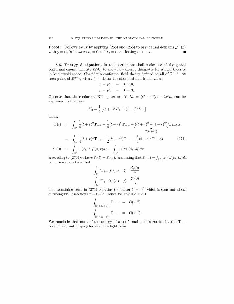
120 3. EQUATIONS DERIVED BY THE VARIATIONAL PRINCIPLE
Proof : Follows easily by applying (265) and (266) to past causal domains J−(p)with p = (t, 0) between t1 = 0 and t2 = t and letting t→ +∞.
3.5. Energy dissipation. In this section we shall make use of the globalconformal energy identity (270) to show how energy dissipates for a filed theoriesin Minkowski space. Consider a conformal field theory defined on all of Rn+1. Ateach point of Rn+1, with t ≥ 0, define the standard null frame where
L = E+ = ∂t + ∂r
L = E− = ∂t − ∂r.
Observe that the conformal Killing vectorfield K0 = (t2 + r2)∂t + 2rt∂r can beexpressed in the form,
K0 =12[(t+ r)2E+ + (t− r)2E−.
]Thus,
Ec(t) =∫
Rn
14(t+ r)2T++ +
14(t− r)2T−− +
((t+ r)2 + (t− r)2
)︸ ︷︷ ︸2(t2+r2)
T+−dx.
=∫
Rn
14(t+ r)2T++ +
12(t2 + r2)T+− +
14(t− r)2T−−dx (271)
Ec(0) =∫
Rn
T(∂t,K0)(0, x)dx =∫
Rn
|x|2T(∂t, ∂t)dx
According to (270) we have Ec(t) = Ec(0). Assuming that Ec(0) =∫
Rn |x|2T(∂t, ∂t)dxis finite we conclude that, ∫
Rn
T++(t, ·)dx .Ec(0)t2∫
Rn
T+−(t, ·)dx .Ec(0)t2
.
The remaining term in (271) contains the factor (t − r)2 which is constant alongoutgoing null directions r = t+ c. Hence for any 0 < ε < 1∫
|x|>(1+ε)t
T−− = O(t−2)∫|x|<(1−ε)t
T−− = O(t−2).
We conclude that most of the energy of a conformal field is carried by the T−−component and propagates near the light cone.
![arXiv · 2018. 8. 3. · arXiv:math/0309459v1 [math.AP] 29 Sep 2003 SHARP TRACE THEOREMS FOR NULL HYPERSURFACES ON EINSTEIN METRICS WITH FINITE CURVATURE FLUX SERGIU KLAINERMAN AND](https://static.documents.pub/doc/80x56/609b04e80b2b1a041a45a8a7/arxiv-2018-8-3-arxivmath0309459v1-mathap-29-sep-2003-sharp-trace-theorems.jpg)


