
Durrell Rittenberg, Ph.D.
Leveraging STAR-CCM+
for Aircraft Applications
Icing in aerospace
– Common applications
– Impact of icing on Aircraft safety
– Common icing conditions and Mechanism of ice accretion
– Types of ice accretion and impact of aerodynamic performance
Leveraging simulation for ice accretion prediction
– Ice Accretion Simulation Considerations
– Physics
Icing and FAA certification
– Changes to the FAA Icing certification regulations
– Impact to Airplane makers
Overview of Icing with STAR-CCM+
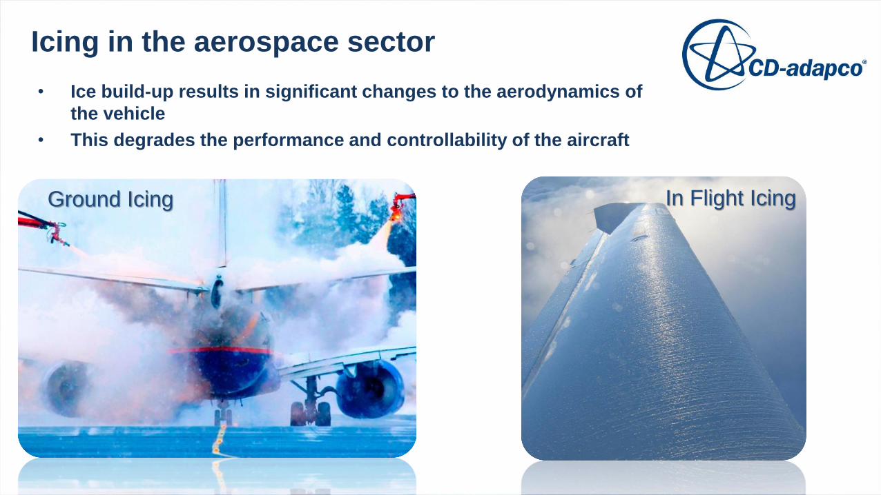
• Ice build-up results in significant changes to the aerodynamics of
the vehicle
• This degrades the performance and controllability of the aircraft
Icing in the aerospace sector
Ground Icing In Flight Icing
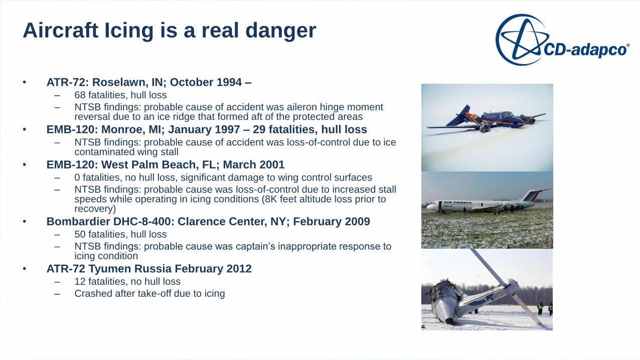
• ATR-72: Roselawn, IN; October 1994 –– 68 fatalities, hull loss
– NTSB findings: probable cause of accident was aileron hinge moment reversal due to an ice ridge that formed aft of the protected areas
• EMB-120: Monroe, MI; January 1997 – 29 fatalities, hull loss – NTSB findings: probable cause of accident was loss-of-control due to ice
contaminated wing stall
• EMB-120: West Palm Beach, FL; March 2001 – 0 fatalities, no hull loss, significant damage to wing control surfaces
– NTSB findings: probable cause was loss-of-control due to increased stall speeds while operating in icing conditions (8K feet altitude loss prior to recovery)
• Bombardier DHC-8-400: Clarence Center, NY; February 2009 – 50 fatalities, hull loss
– NTSB findings: probable cause was captain’s inappropriate response to icing condition
• ATR-72 Tyumen Russia February 2012– 12 fatalities, no hull loss
– Crashed after take-off due to icing
Aircraft Icing is a real danger
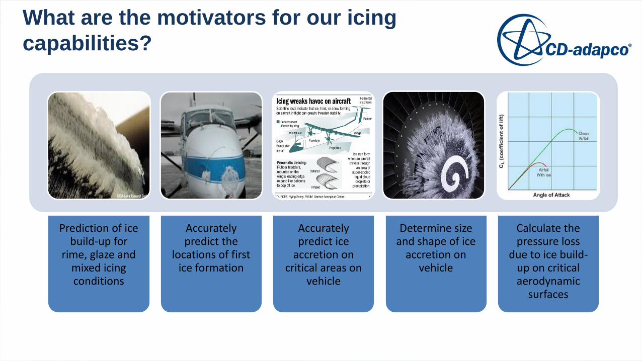
Prediction of ice build-up for
rime, glaze and mixed icing conditions
Accurately predict the
locations of first ice formation
Accurately predict ice
accretion on critical areas on
vehicle
Determine size and shape of ice
accretion on vehicle
Calculate the pressure loss
due to ice build-up on critical aerodynamic
surfaces
What are the motivators for our icing
capabilities?
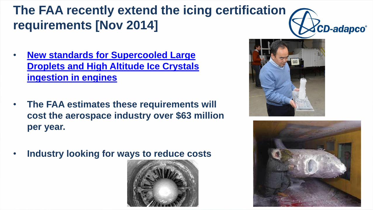
• New standards for Supercooled Large
Droplets and High Altitude Ice Crystals
ingestion in engines
• The FAA estimates these requirements will
cost the aerospace industry over $63 million
per year.
• Industry looking for ways to reduce costs
The FAA recently extend the icing certification
requirements [Nov 2014]
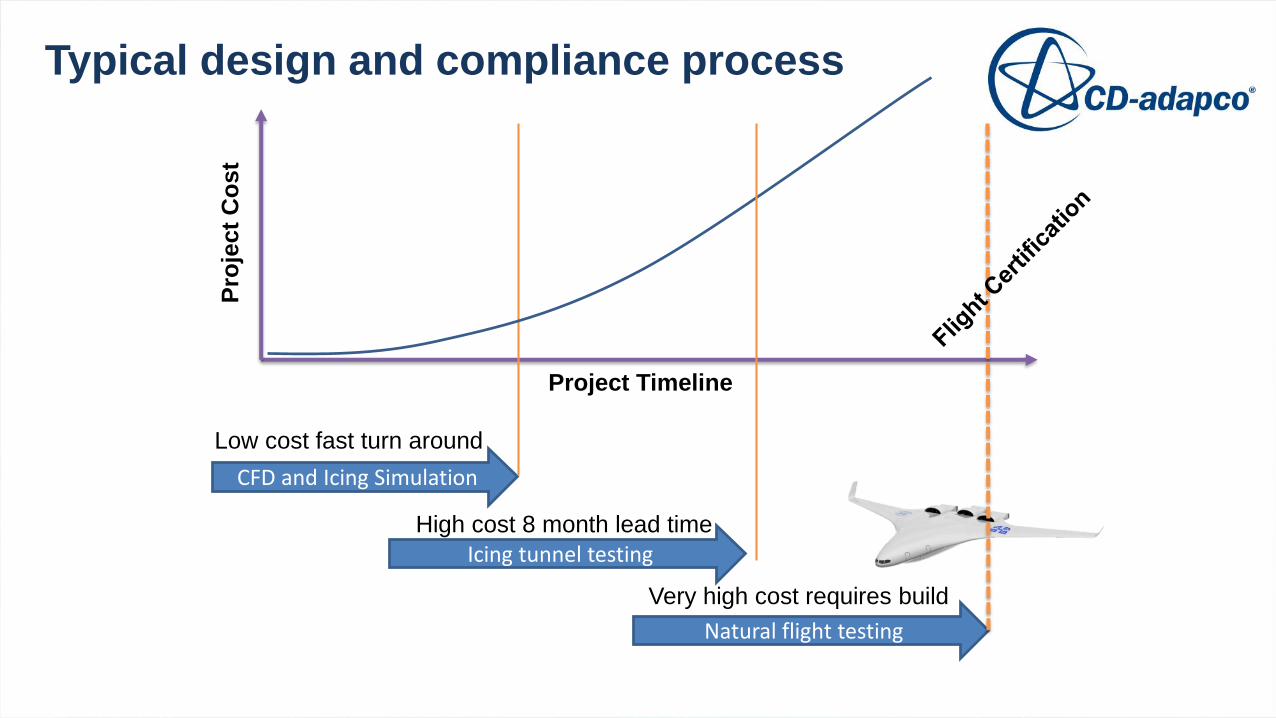
Typical design and compliance process
CFD and Icing Simulation
Low cost fast turn around
Pro
ject
Co
st
Icing tunnel testingHigh cost 8 month lead time
Project Timeline
Natural flight testing
Very high cost requires build
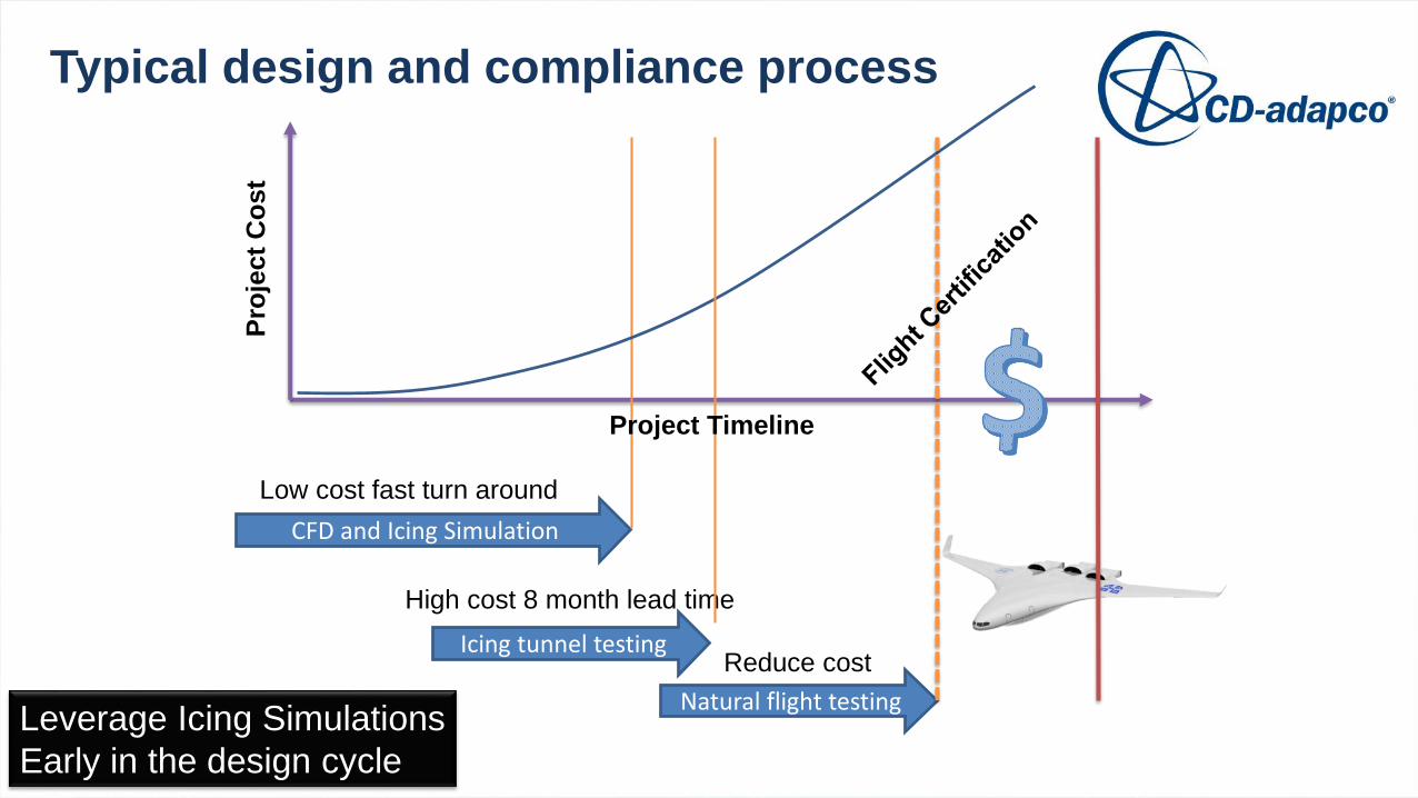
Typical design and compliance process
CFD and Icing Simulation
Low cost fast turn around
Pro
ject
Co
st
Icing tunnel testing
High cost 8 month lead time
Project Timeline
Natural flight testing
Reduce cost
Leverage Icing Simulations
Early in the design cycle
The basics of ice accretion and
aircraft icing
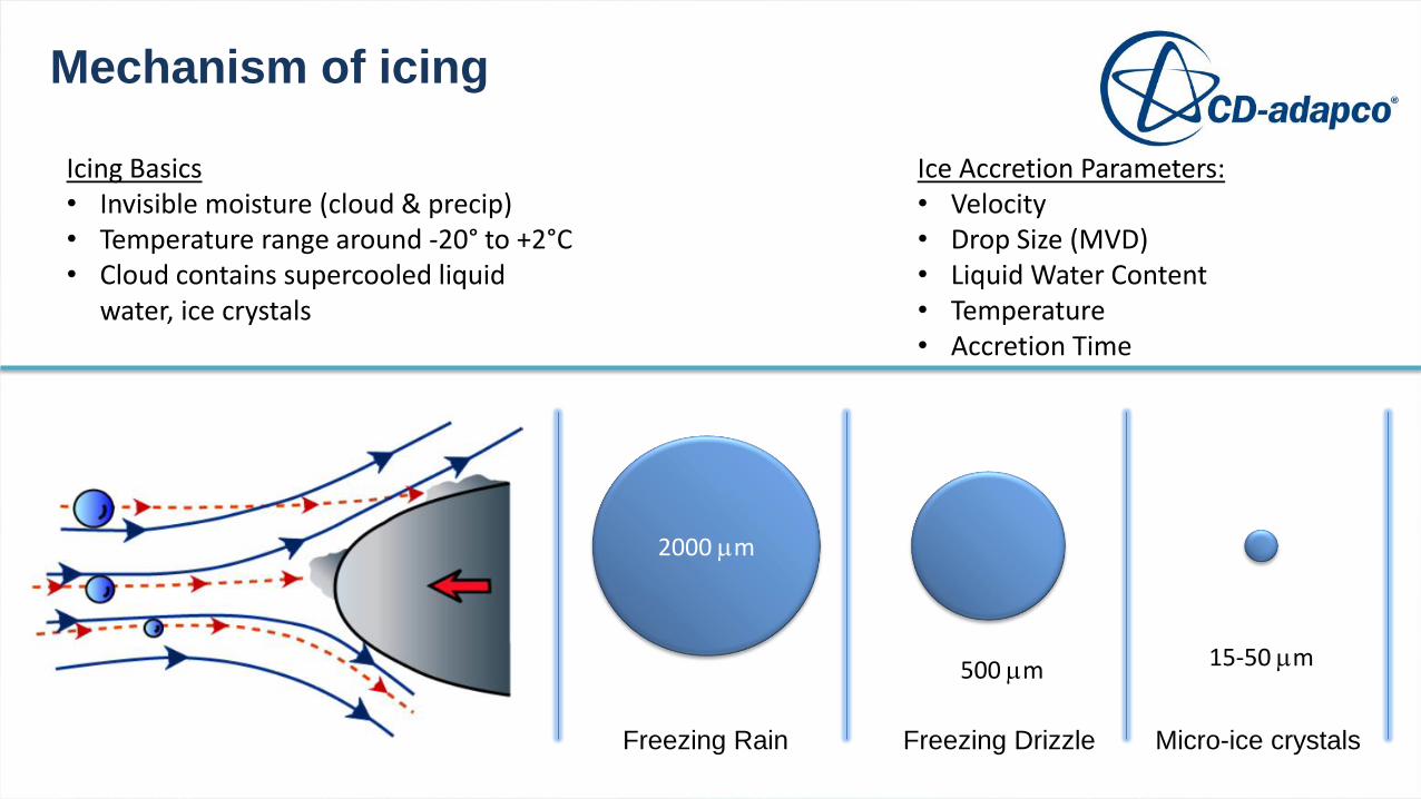
Mechanism of icing
Icing Basics• Invisible moisture (cloud & precip) • Temperature range around -20° to +2°C • Cloud contains supercooled liquid
water, ice crystals
Ice Accretion Parameters: • Velocity• Drop Size (MVD)• Liquid Water Content• Temperature • Accretion Time
2000 mm
Freezing Rain Freezing Drizzle Micro-ice crystals
15-50 mm500 mm
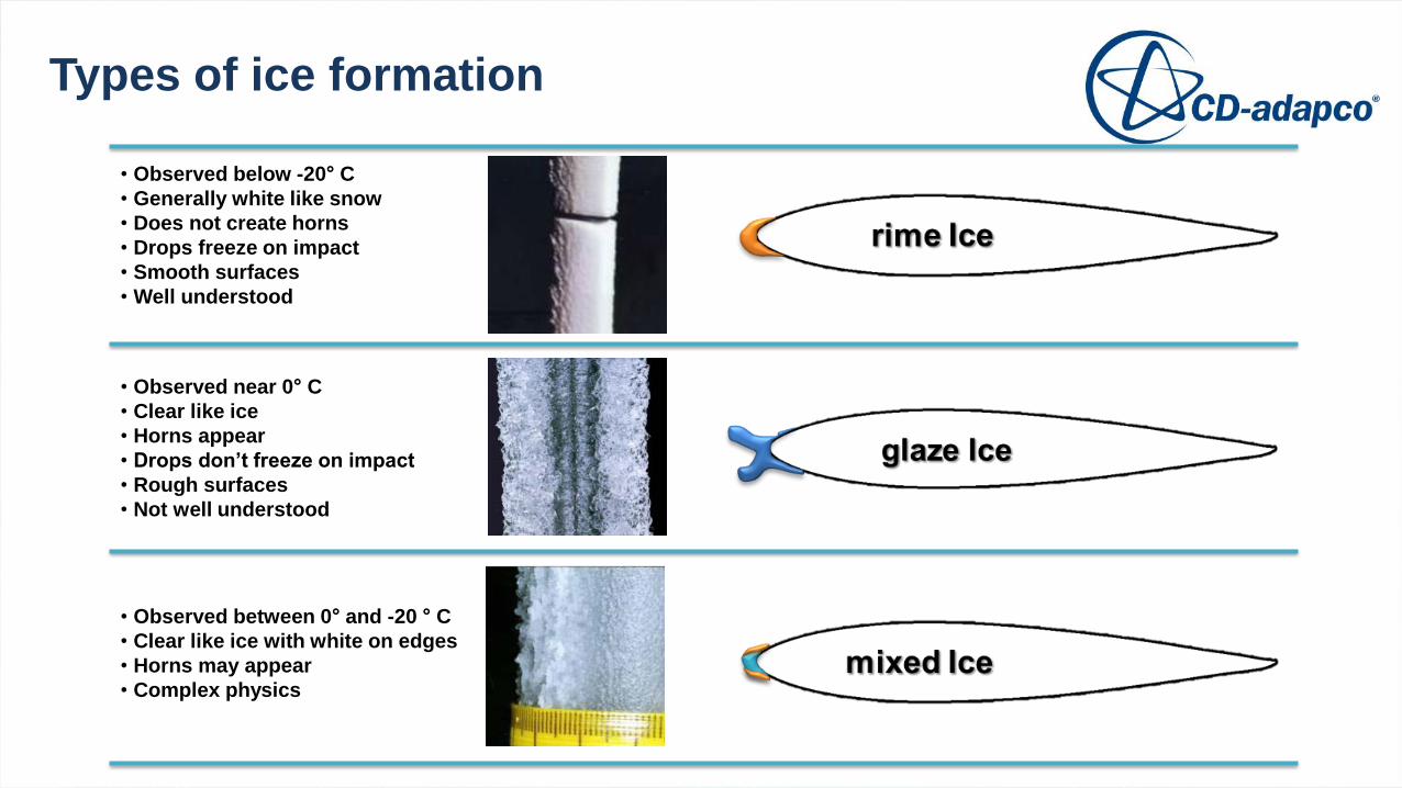
Types of ice formation
• Observed below -20° C
• Generally white like snow
• Does not create horns
• Drops freeze on impact
• Smooth surfaces
• Well understood
• Observed near 0° C
• Clear like ice
• Horns appear
• Drops don’t freeze on impact
• Rough surfaces
• Not well understood
• Observed between 0° and -20 ° C
• Clear like ice with white on edges
• Horns may appear
• Complex physics
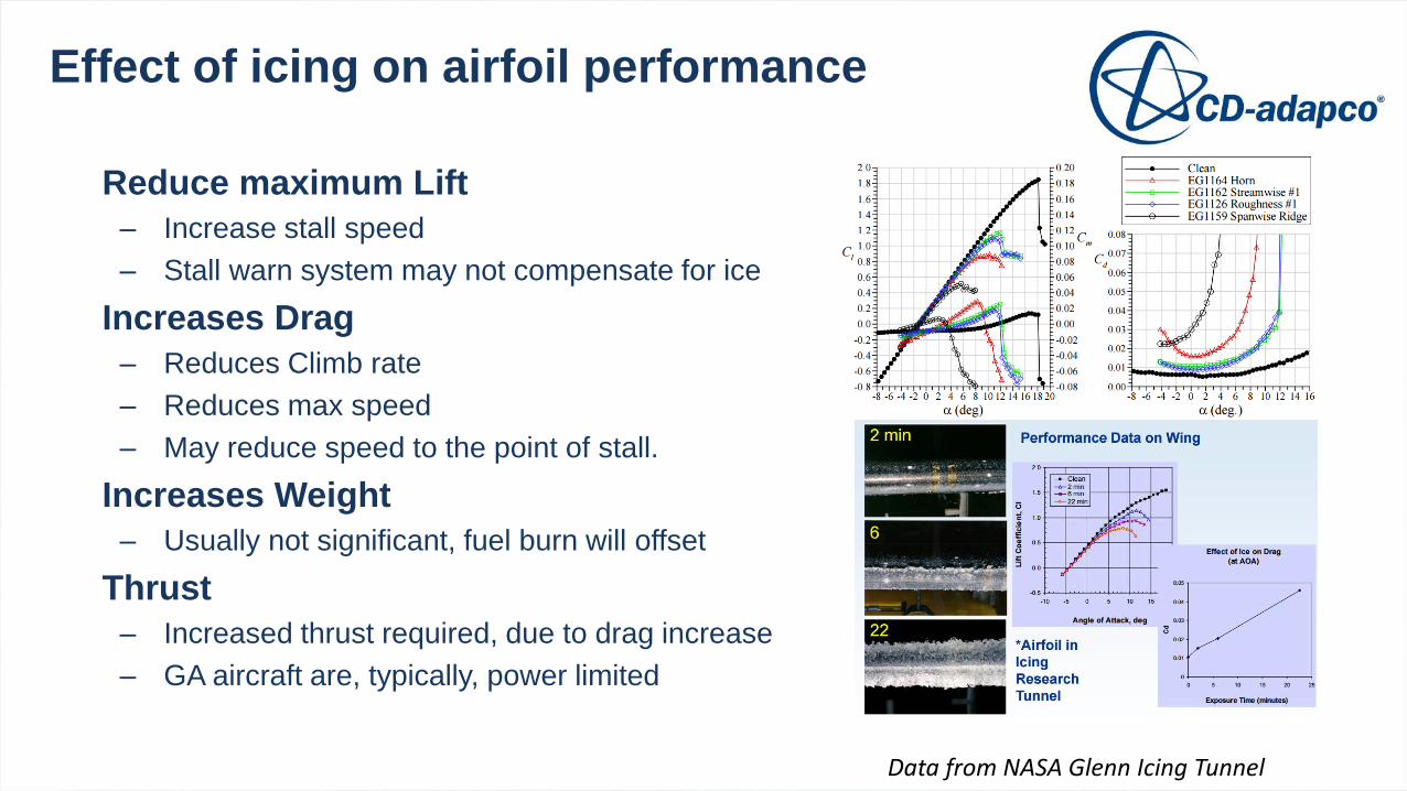
Reduce maximum Lift
– Increase stall speed
– Stall warn system may not compensate for ice
Increases Drag
– Reduces Climb rate
– Reduces max speed
– May reduce speed to the point of stall.
Increases Weight
– Usually not significant, fuel burn will offset
Thrust
– Increased thrust required, due to drag increase
– GA aircraft are, typically, power limited
Effect of icing on airfoil performance
Data from NASA Glenn Icing Tunnel
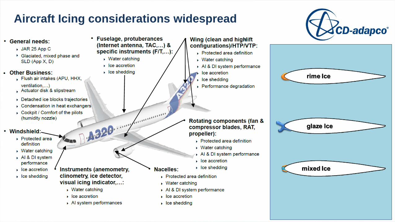
Aircraft Icing considerations widespread
Ice Accretion Simulation
ConsiderationsThe Physics of Ice Accretion with formulations
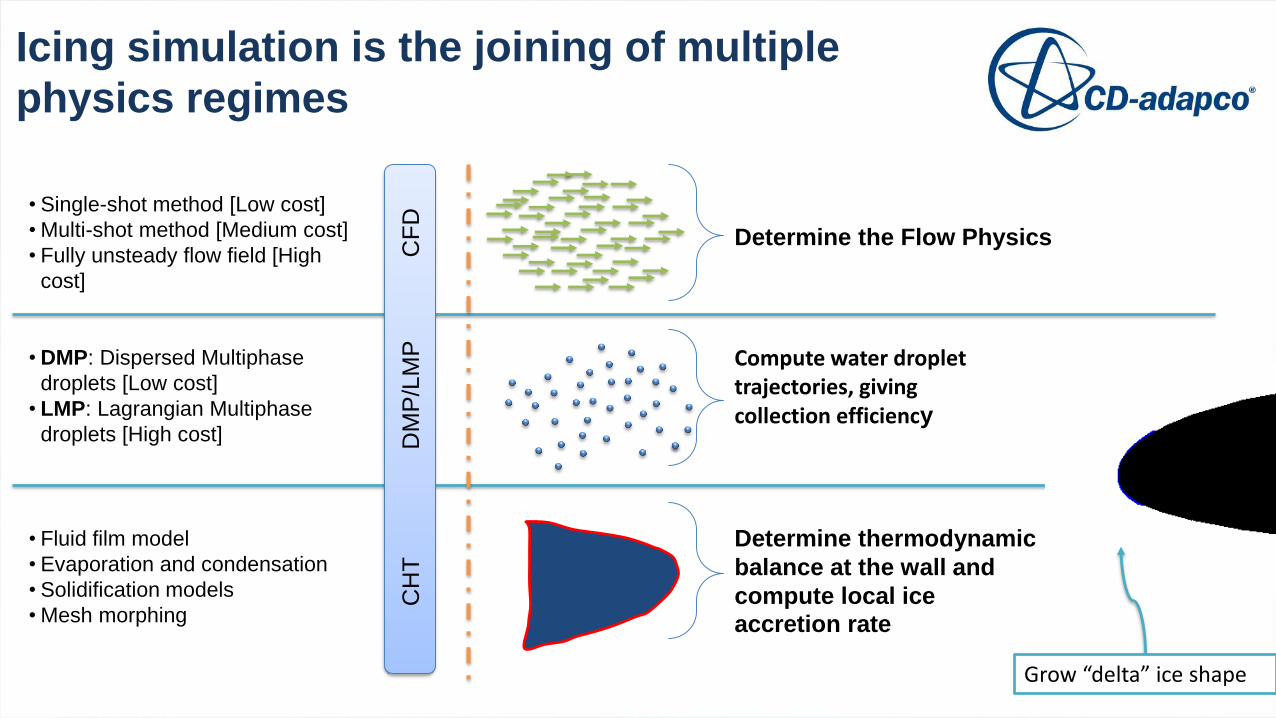
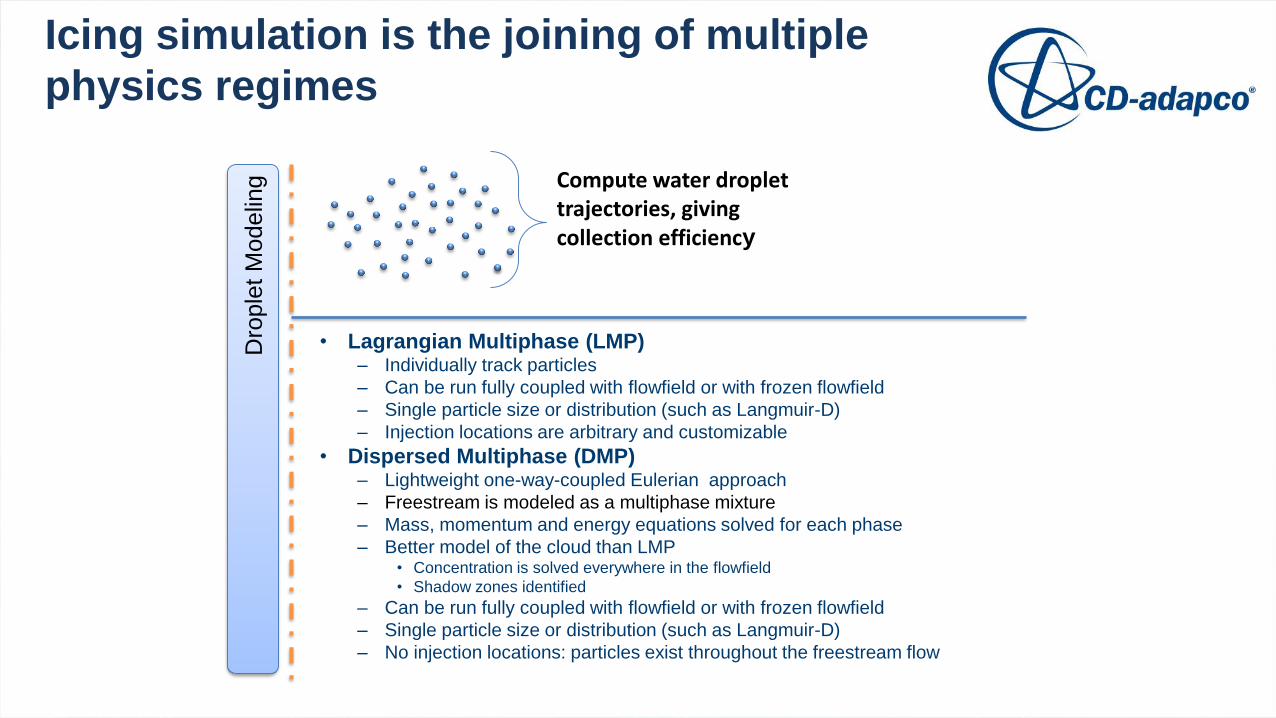
Icing simulation is the joining of multiple
physics regimes
Determine the Flow Physics
Compute water droplet trajectories, giving collection efficiency
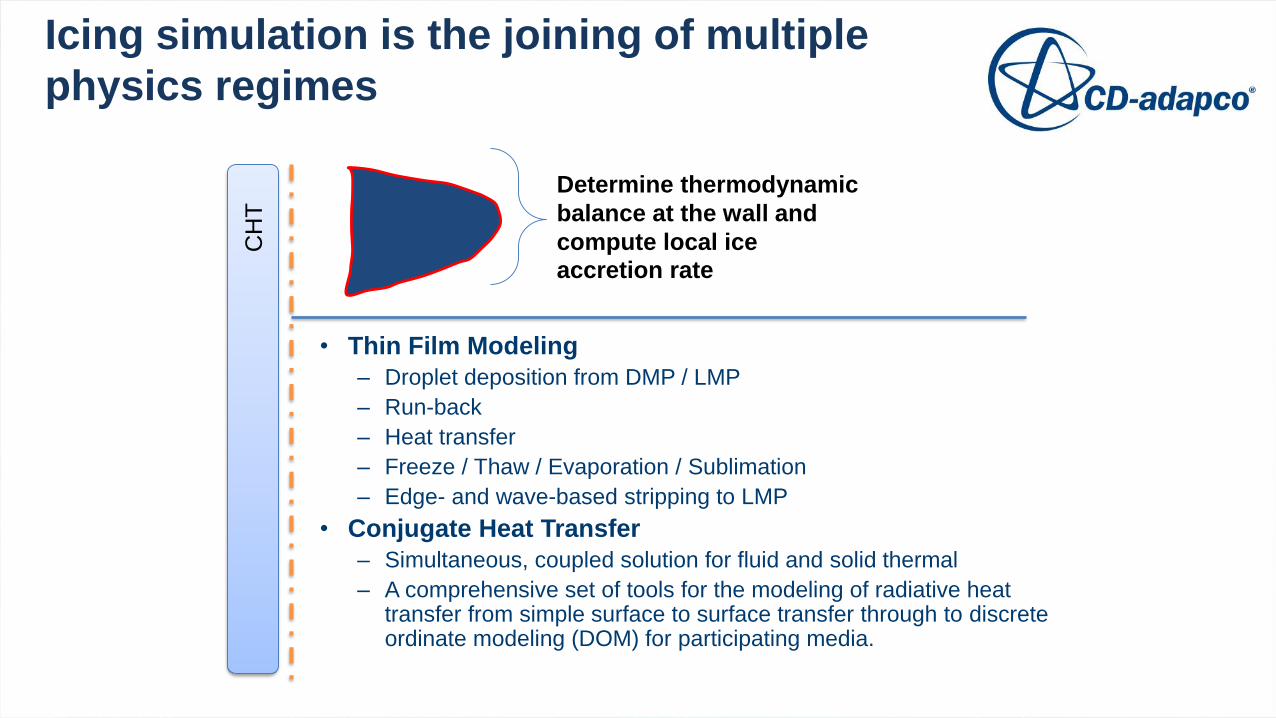
Determine thermodynamic
balance at the wall and
compute local ice
accretion rate
CF
DD
MP
/LM
PC
HT
Grow “delta” ice shape
• Single-shot method [Low cost]
• Multi-shot method [Medium cost]
• Fully unsteady flow field [High
cost]
• DMP: Dispersed Multiphase
droplets [Low cost]
• LMP: Lagrangian Multiphase
droplets [High cost]
• Fluid film model
• Evaporation and condensation
• Solidification models
• Mesh morphing
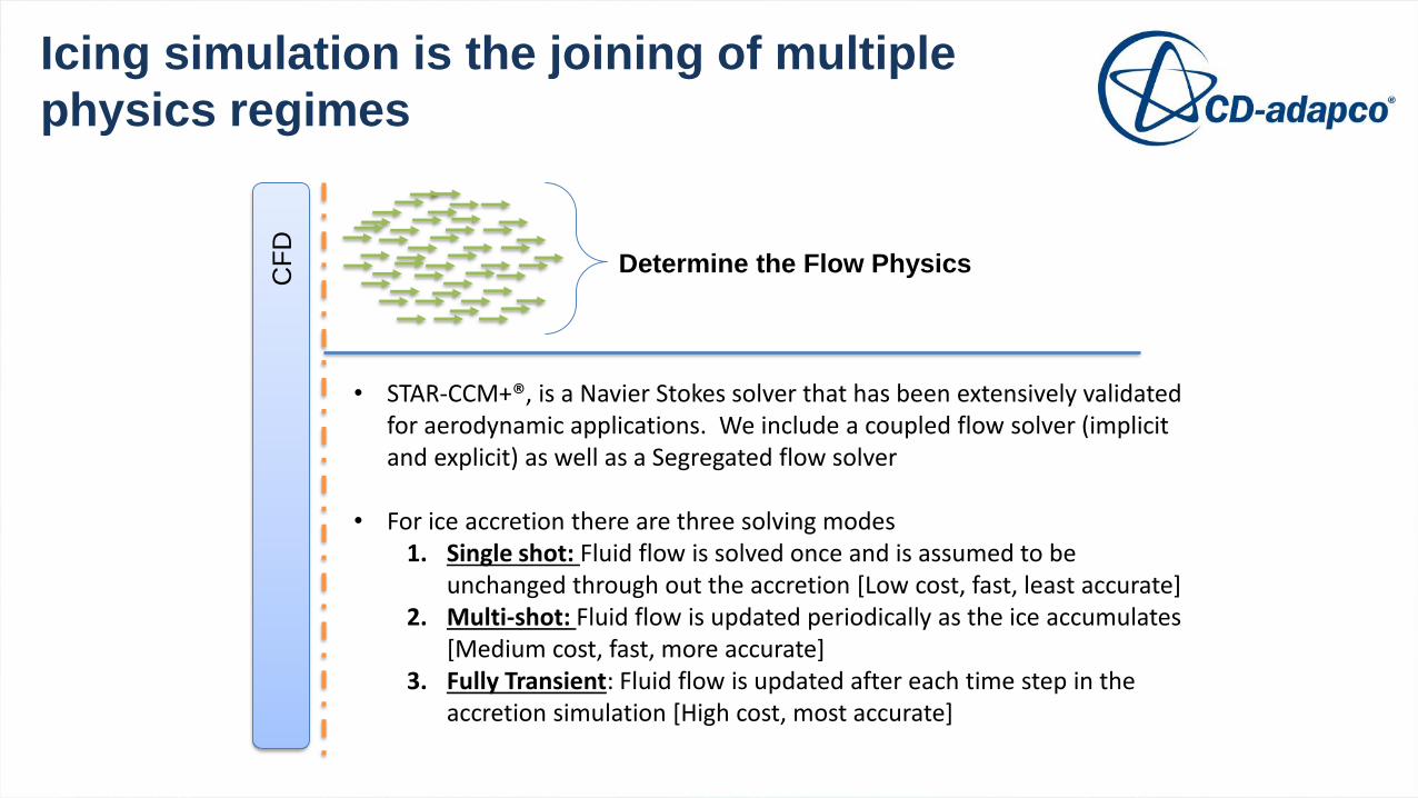
Icing simulation is the joining of multiple
physics regimes
Determine the Flow PhysicsC
FD
• STAR-CCM+®, is a Navier Stokes solver that has been extensively validated for aerodynamic applications. We include a coupled flow solver (implicit and explicit) as well as a Segregated flow solver
• For ice accretion there are three solving modes1. Single shot: Fluid flow is solved once and is assumed to be
unchanged through out the accretion [Low cost, fast, least accurate]2. Multi-shot: Fluid flow is updated periodically as the ice accumulates
[Medium cost, fast, more accurate]3. Fully Transient: Fluid flow is updated after each time step in the
accretion simulation [High cost, most accurate]
Icing simulation is the joining of multiple
physics regimes
Compute water droplet trajectories, giving collection efficiency
Dro
ple
t M
odelin
g
• Lagrangian Multiphase (LMP)– Individually track particles
– Can be run fully coupled with flowfield or with frozen flowfield
– Single particle size or distribution (such as Langmuir-D)
– Injection locations are arbitrary and customizable
• Dispersed Multiphase (DMP)– Lightweight one-way-coupled Eulerian approach
– Freestream is modeled as a multiphase mixture
– Mass, momentum and energy equations solved for each phase
– Better model of the cloud than LMP• Concentration is solved everywhere in the flowfield
• Shadow zones identified
– Can be run fully coupled with flowfield or with frozen flowfield
– Single particle size or distribution (such as Langmuir-D)
– No injection locations: particles exist throughout the freestream flow
Icing simulation is the joining of multiple
physics regimes
Determine thermodynamic
balance at the wall and
compute local ice
accretion rateC
HT
• Thin Film Modeling
– Droplet deposition from DMP / LMP
– Run-back
– Heat transfer
– Freeze / Thaw / Evaporation / Sublimation
– Edge- and wave-based stripping to LMP
• Conjugate Heat Transfer
– Simultaneous, coupled solution for fluid and solid thermal
– A comprehensive set of tools for the modeling of radiative heat transfer from simple surface to surface transfer through to discrete ordinate modeling (DOM) for participating media.
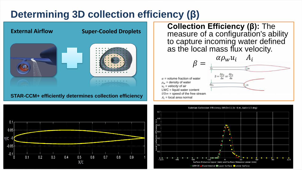
STAR-CCM+ efficiently determines collection efficiency
Collection Efficiency (β): The measure of a configuration's ability to capture incoming water defined as the local mass flux velocity.
𝛽 =𝛼𝜌𝑤𝑢𝑖𝐿𝑊𝐶 𝑈∞
𝐴𝑖|𝐴|
𝛼 = volume fraction of water
𝜌𝑤 = density of water
𝑢𝑖 = velocity of air
LWC = liquid water content
𝑈∞ = speed of the free stream
𝐴𝑖 = local area normal
Determining 3D collection efficiency (β)
External Airflow Super-Cooled Droplets
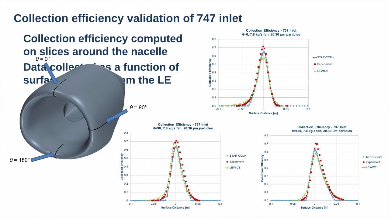
Collection efficiency computed
on slices around the nacelle
Data collected as a function of
surface distance from the LE
Collection efficiency validation of 747 inlet
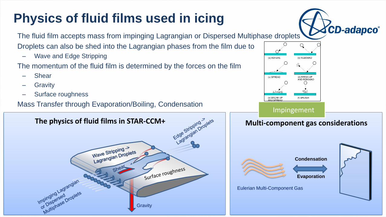
Physics of fluid films used in icing
The fluid film accepts mass from impinging Lagrangian or Dispersed Multiphase droplets
Droplets can also be shed into the Lagrangian phases from the film due to
– Wave and Edge Stripping
The momentum of the fluid film is determined by the forces on the film
– Shear
– Gravity
– Surface roughness
Mass Transfer through Evaporation/Boiling, Condensation
Gravity
Eulerian Multi-Component Gas
Condensation
Evaporation
Impingement
Multi-component gas considerationsThe physics of fluid films in STAR-CCM+
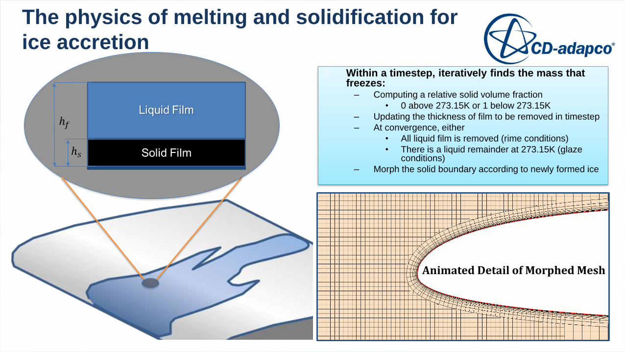
Within a timestep, iteratively finds the mass that freezes:
– Computing a relative solid volume fraction
• 0 above 273.15K or 1 below 273.15K
– Updating the thickness of film to be removed in timestep
– At convergence, either
• All liquid film is removed (rime conditions)
• There is a liquid remainder at 273.15K (glaze conditions)
– Morph the solid boundary according to newly formed ice
The physics of melting and solidification for
ice accretion
Animated Detail of Morphed Mesh
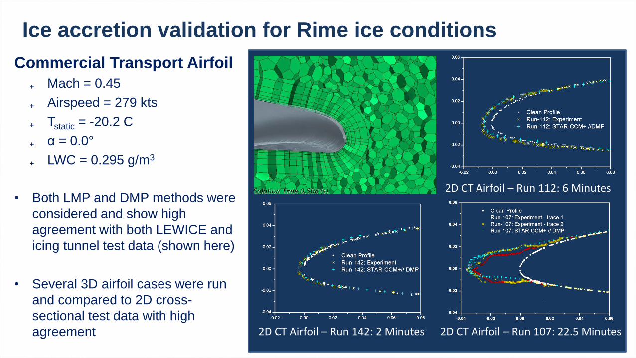
Ice accretion validation for Rime ice conditions
2D CT Airfoil – Run 142: 2 Minutes
2D CT Airfoil – Run 112: 6 Minutes
2D CT Airfoil – Run 107: 22.5 Minutes
Commercial Transport Airfoil
₊ Mach = 0.45
₊ Airspeed = 279 kts
₊ Tstatic = -20.2 C
₊ α = 0.0°
₊ LWC = 0.295 g/m3
• Both LMP and DMP methods were
considered and show high
agreement with both LEWICE and
icing tunnel test data (shown here)
• Several 3D airfoil cases were run
and compared to 2D cross-
sectional test data with high
agreement
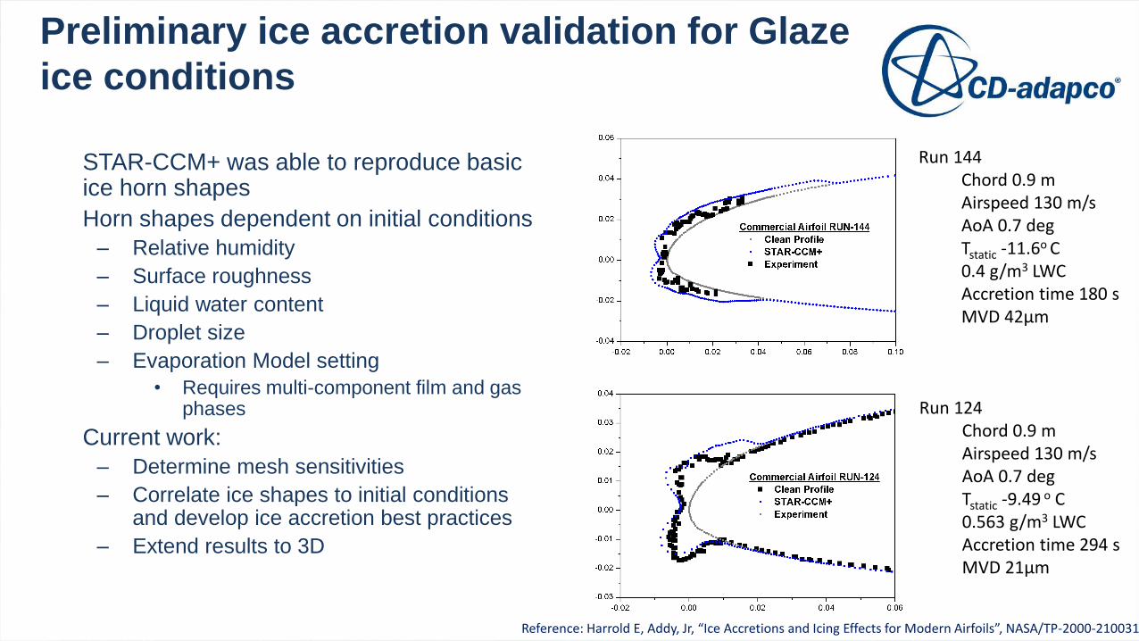
STAR-CCM+ was able to reproduce basic ice horn shapes
Horn shapes dependent on initial conditions
– Relative humidity
– Surface roughness
– Liquid water content
– Droplet size
– Evaporation Model setting
• Requires multi-component film and gas phases
Current work:
– Determine mesh sensitivities
– Correlate ice shapes to initial conditions and develop ice accretion best practices
– Extend results to 3D
Preliminary ice accretion validation for Glaze
ice conditions
Run 124Chord 0.9 mAirspeed 130 m/sAoA 0.7 degTstatic -9.49 o C0.563 g/m3 LWCAccretion time 294 sMVD 21μm
Run 144Chord 0.9 mAirspeed 130 m/sAoA 0.7 degTstatic -11.6o C0.4 g/m3 LWCAccretion time 180 sMVD 42μm
Reference: Harrold E, Addy, Jr, “Ice Accretions and Icing Effects for Modern Airfoils”, NASA/TP-2000-210031
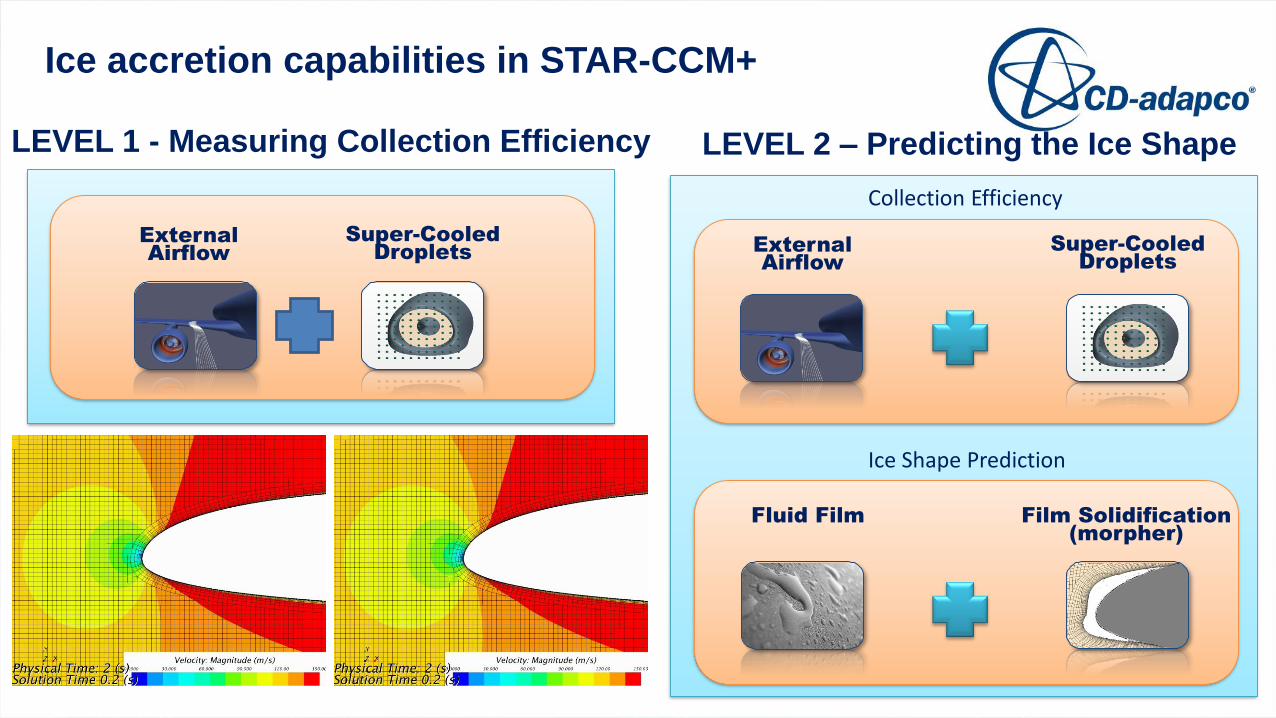
Ice accretion capabilities in STAR-CCM+
LEVEL 1 - Measuring Collection Efficiency
External
Airflow
Super-Cooled
DropletsExternal
Airflow
Super-Cooled
Droplets
Fluid Film Film Solidification
(morpher)
LEVEL 2 – Predicting the Ice Shape
Collection Efficiency
Ice Shape Prediction
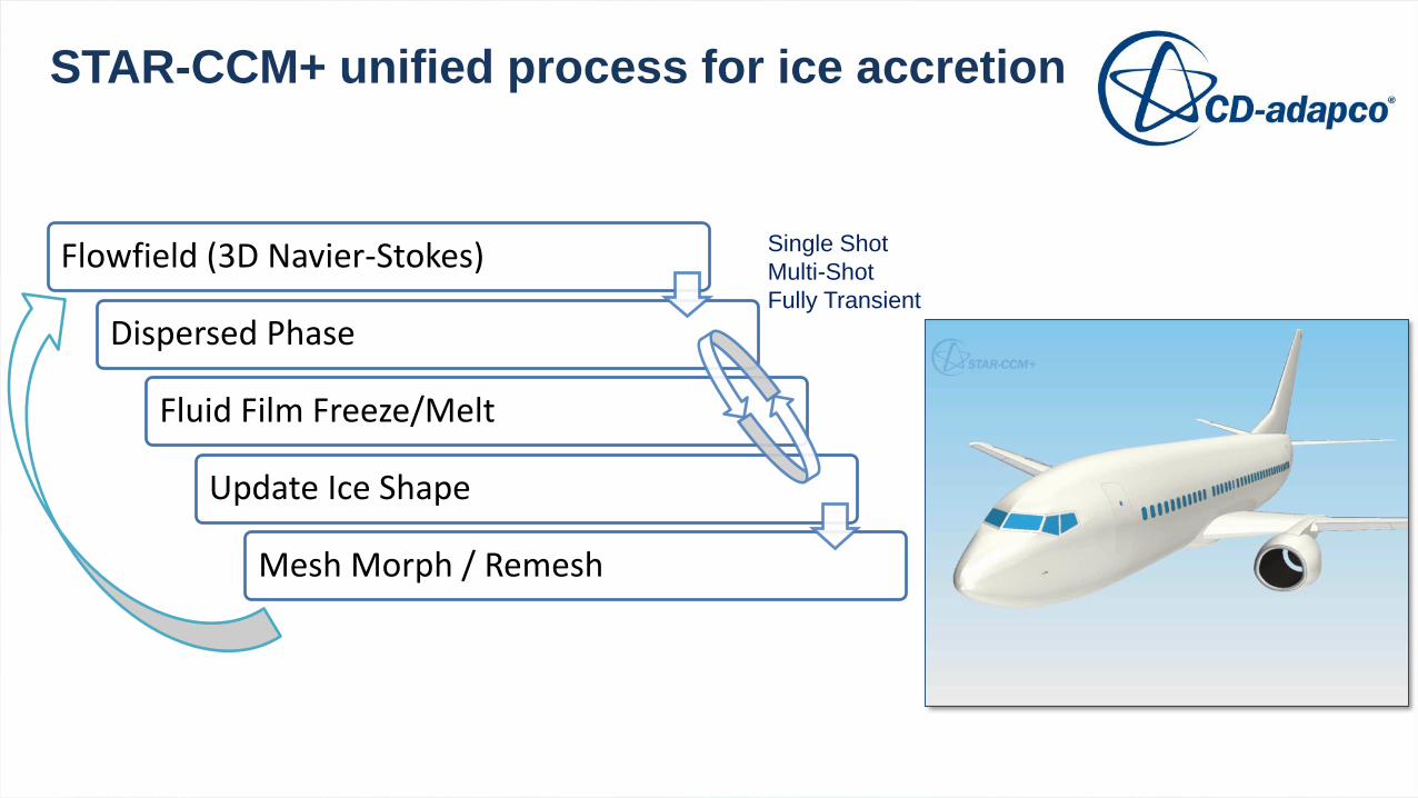
STAR-CCM+ unified process for ice accretion
Flowfield (3D Navier-Stokes)
Dispersed Phase
Fluid Film Freeze/Melt
Update Ice Shape
Mesh Morph / Remesh
Single Shot
Multi-Shot
Fully Transient
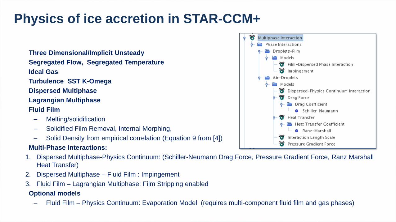
Three Dimensional/Implicit Unsteady
Segregated Flow, Segregated Temperature
Ideal Gas
Turbulence SST K-Omega
Dispersed Multiphase
Lagrangian Multiphase
Fluid Film
– Melting/solidification
– Solidified Film Removal, Internal Morphing,
– Solid Density from empirical correlation (Equation 9 from [4])
Multi-Phase Interactions:
1. Dispersed Multiphase-Physics Continuum: (Schiller-Neumann Drag Force, Pressure Gradient Force, Ranz Marshall
Heat Transfer)
2. Dispersed Multiphase – Fluid Film : Impingement
3. Fluid Film – Lagrangian Multiphase: Film Stripping enabled
Optional models
– Fluid Film – Physics Continuum: Evaporation Model (requires multi-component fluid film and gas phases)
Physics of ice accretion in STAR-CCM+
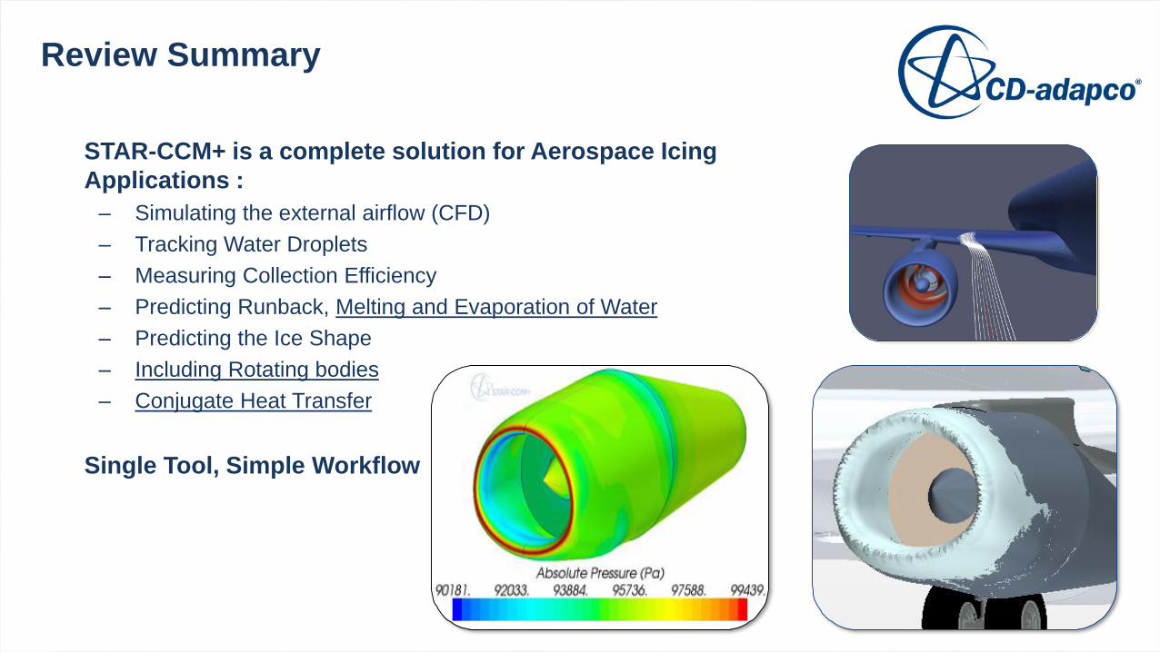
STAR-CCM+ is a complete solution for Aerospace Icing
Applications :
– Simulating the external airflow (CFD)
– Tracking Water Droplets
– Measuring Collection Efficiency
– Predicting Runback, Melting and Evaporation of Water
– Predicting the Ice Shape
– Including Rotating bodies
– Conjugate Heat Transfer
Single Tool, Simple Workflow
Review Summary
Appendix and other
technical details
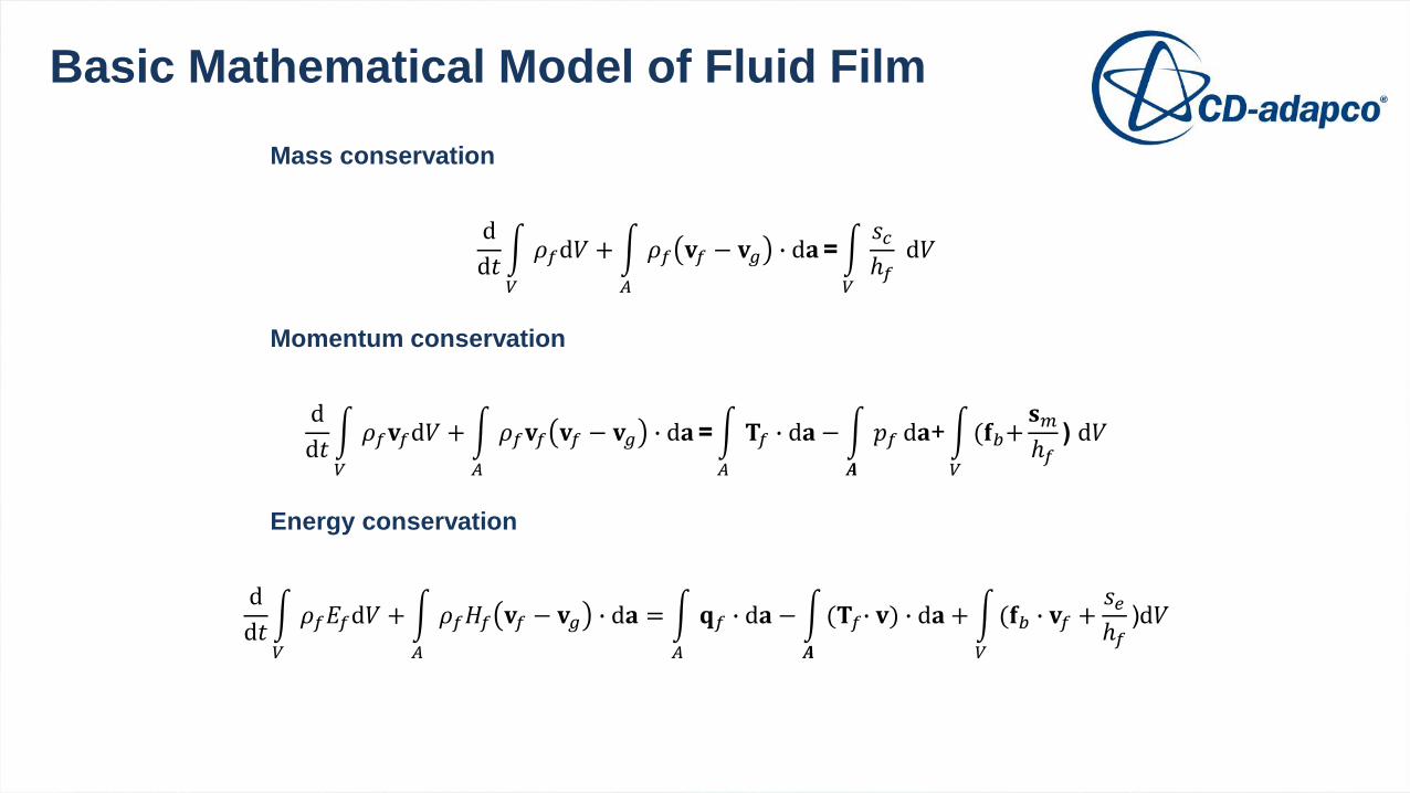
Mass conservation
d
d𝑡න
𝑉
𝜌𝑓d𝑉 + න
𝐴
𝜌𝑓 𝐯𝑓 − 𝐯𝑔 ∙ d𝐚=න
𝑉
𝑠𝑐ℎ𝑓
d𝑉
Momentum conservation
d
d𝑡න
𝑉
𝜌𝑓𝐯𝑓d𝑉 + න
𝐴
𝜌𝑓𝐯𝑓 𝐯𝑓 − 𝐯𝑔 ∙ d𝐚=න
𝐴
𝐓𝑓 ∙ d𝐚 − න
𝑨
𝑝𝑓 d𝐚+න
𝑉
(𝐟𝑏+𝐬𝑚ℎ𝑓
) d𝑉
Energy conservation
d
d𝑡න
𝑉
𝜌𝑓𝐸𝑓d𝑉 + න
𝐴
𝜌𝑓𝐻𝑓 𝐯𝑓 − 𝐯𝑔 ∙ d𝐚 = න
𝐴
𝐪𝑓 ∙ d𝐚 − න
𝑨
(𝐓𝑓∙ 𝐯) ∙ d𝐚 + න
𝑉
(𝐟𝑏 ∙ 𝐯𝑓 +𝑠𝑒ℎ𝑓
)d𝑉
Basic Mathematical Model of Fluid Film
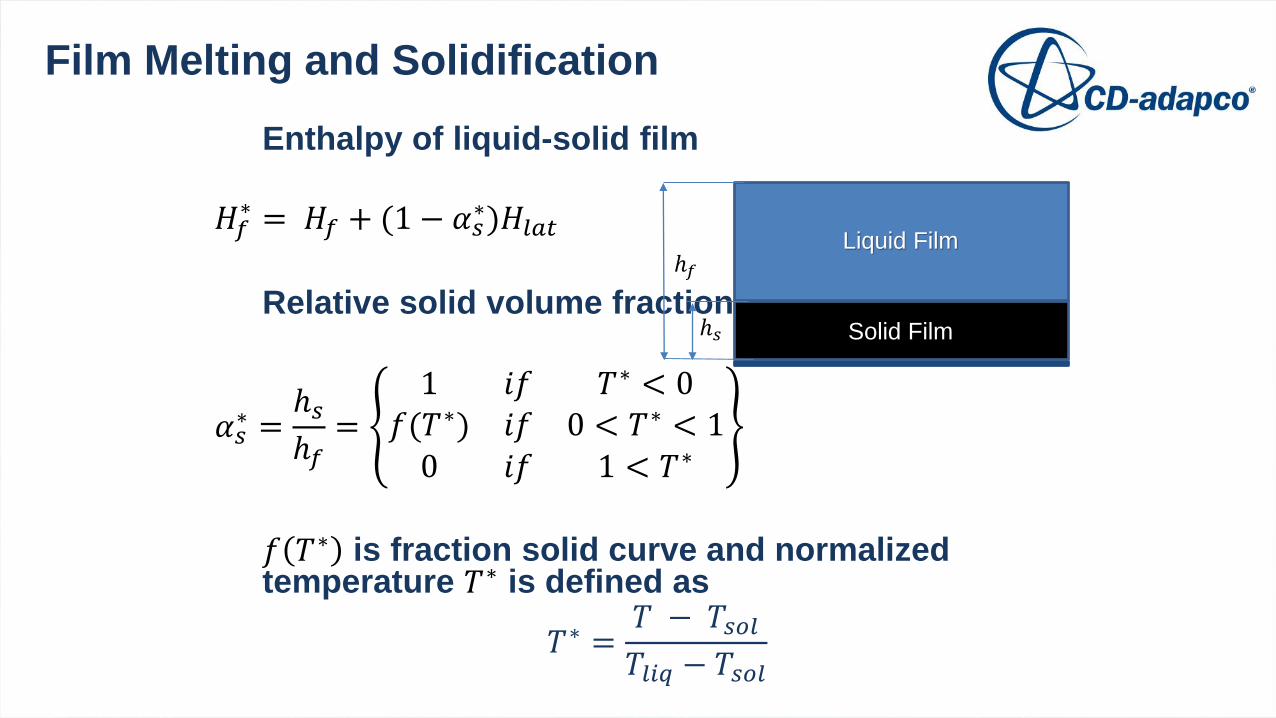
Enthalpy of liquid-solid film
𝐻𝑓∗ = 𝐻𝑓 + (1 − 𝛼𝑠
∗)𝐻𝑙𝑎𝑡
Relative solid volume fraction
𝛼𝑠∗ =
ℎ𝑠ℎ𝑓
=
1 𝑖𝑓 𝑇∗ < 0𝑓(𝑇∗) 𝑖𝑓 0 < 𝑇∗ < 1
0 𝑖𝑓 1 < 𝑇∗
𝑓 𝑇∗ is fraction solid curve and normalized temperature 𝑇∗ is defined as
𝑇∗ =𝑇 − 𝑇𝑠𝑜𝑙𝑇𝑙𝑖𝑞 − 𝑇𝑠𝑜𝑙
Film Melting and Solidification
Liquid Film
Solid Film
ℎ𝑓
ℎ𝑠
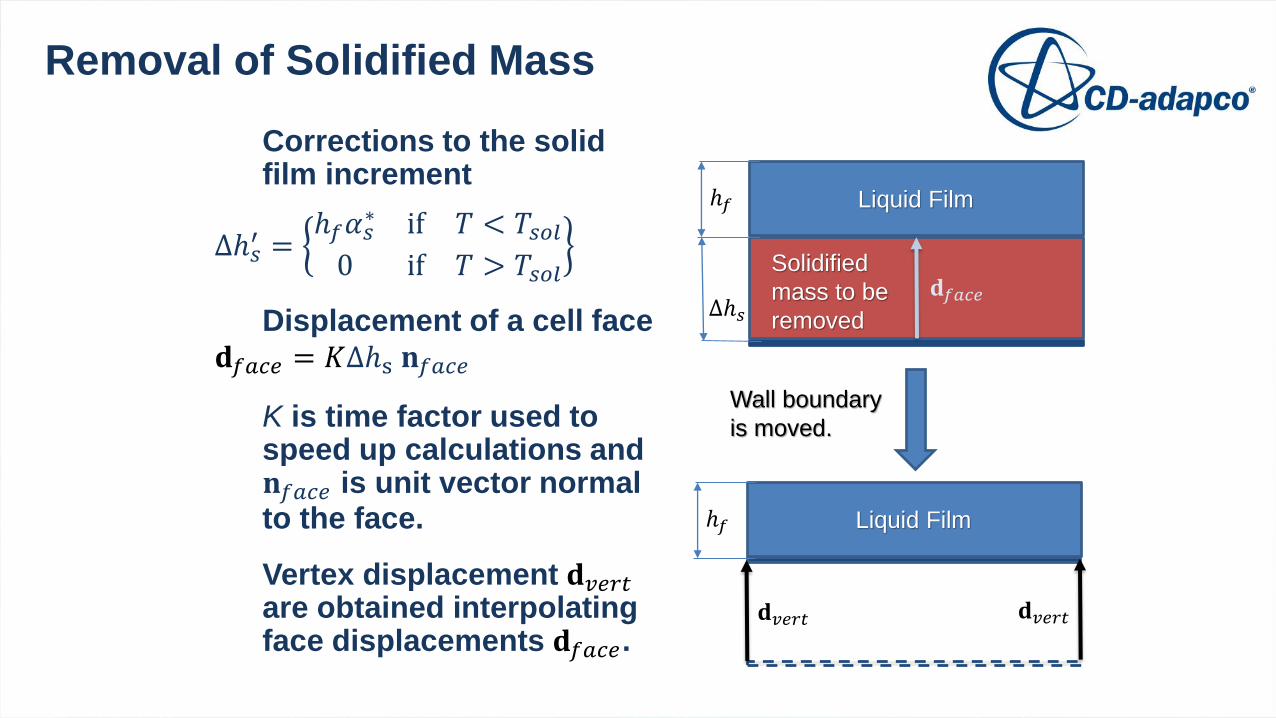
Corrections to the solid film increment
∆ℎ𝑠′ =
ℎ𝑓𝛼𝑠∗ if 𝑇 < 𝑇𝑠𝑜𝑙
0 if 𝑇 > 𝑇𝑠𝑜𝑙
Displacement of a cell face
𝐝𝑓𝑎𝑐𝑒 = 𝐾∆ℎs 𝐧𝑓𝑎𝑐𝑒
K is time factor used to speed up calculations and 𝐧𝑓𝑎𝑐𝑒 is unit vector normal to the face.
Vertex displacement 𝐝𝑣𝑒𝑟𝑡are obtained interpolating face displacements 𝐝𝑓𝑎𝑐𝑒.
Removal of Solidified Mass
Liquid Filmℎ𝑓
∆ℎ𝑠
Solidified
mass to be
removed
𝐝𝑓𝑎𝑐𝑒
Wall boundary
is moved.
Liquid Film
𝐝𝑣𝑒𝑟𝑡 𝐝𝑣𝑒𝑟𝑡
ℎ𝑓


