
AD-A248 641lilI li I 'Illi I'II'llII lI II
NAVAL POSTGRADUATE SCHOOLMonterey, California
' G I D -1DTIC
SFLECTESAPR17 1992 THESISD
AUTOMATED PERFORMANCEEVALUATION TECHNIQUE
by
Brian E. Skimmons
March 1992
Thesis Advisor: Donald V.Z. Wadsworth
Approved for public release; distribution is unlimited
92-09837

UNCLASSI FI EDSECURITY CLASS
'X (A' :C". O
. '- S PAE
f€orm ApprovedI
REPORT DOCUMENTATION PAGE OMB o 0704 0188
la REPORT SECURITY CLASS F CATIOrt 1o RESTRiCTivE MAR ,,NGS
UNCLASSIFIED2a SECURITY CLASSFiCA" O% AITHOR -Y 3 0 STP B-ThON, 'AV LAB TY 0; PEE
Approved for public release;
2b DECLASSiFICATION i',K,%GRAD % SCHEDULE distribution is unlimited
4 PERFORMING OHG4A\,LZU, REPORT NKMBEqIS; 5 MON'TOR G ORGA ZAT .. R C''- 7.' K'
6a NAME OF PERFORPMANG OZGAN ZATON 6b OFF Ct SYVBO. 7a NAVE OF J". C : O9(A.(If applicable)
Naval Postgraduate School EC Naval Postgraduate School
6c ADDRESS (Ot). State. and ZIP Code) 7D ADDRESS (City State and ZIPCdcde)
Monterey, CA 93943-5000 Monterey, CA 93943-5000
8a 'AVl '.,5 - . S j ;n 0F:CS S' .'s: ' 9 _%D r*o S . Do CA'
ORGAN.ZA' ON j (If applicable)
8c ADDRESS (City State and ZIP Code) c* ,, F",,.
L'%'[% V-) %O N0 A-CCSSON NO
11 7-.E (Include Security Ciassifi arton)
AUTOMATED PERFORMANCE EVALUATION TECHNIQUE'2 Pt;SOAL la,§'")OSI
SKIMMONS, Brian E.1 3a - :E O 0''C
T 3: ''. iO_)CR 4[.,. ;A OF R;FO"P (Yea' Month D) 10.
Master's Thesis . -.- 1992 March 153' F N,. 'A0-. The views expressed in this thesis are those of theauthor and do not reflect the official policy or position of the Depart-ment of Defense or the US Government..7 QC $A ' 8 S',, rT TE '% 'Coat,nue on ,Etse if ntrssar, jn ,d, rt, b) bf cot numnbcr)
D. RFI Mitigation; CDAA Performance; RFDFManagement
j A - O.( Contrue Vqt rev erisE if riecessary and identify by blo(A, nurito r!
The U.S. Navy operates a number of radio receiving and signal collec-tion sites throughout the world. These sites have been modified andupgraded a number of times to incorporate new equipment technology andadvanced receiving and data processing systems. In addition, theencroachment of other activities near the sites has increased the levelsof radio and electrical noise to harmful levels. The impact of somesite modifications and increased noise levels on the ability of the sitesto receive and process data from signals-of-interest (SOIs) is a majorconcern.
A means to evaluate the positive (or negative) impact of site improve-ments, site upgrades, and site encroachment on the performance of a sitehas not been available in past years. To fill this void, a performance
, - ' UNCLASSIFIED
WADSWORTH, Donald V.Z. 408-646-2115 FC!Wr4DD Form 1473, JUN 86 '",' . , . . " .,t)5,0 .
S, ': 1 }l j-II -III -,, UNCLASSIFIED

UNCLASSIFIED'F II l 1 ' .' " IFI '' I I ! l I'.,
19. cont.evaluation technique (PET) was developed by the staff and students ofthe Naval Postgraduate School. PET has gradually evolved into a use-ful analytic tool used during field surveys conducted by the Signal-to-Noise Enhancement Program (SNEP). SNEP teams visit selected sites toassess the impact of site modifications and man-made ratio noise on thereception of SOIs. The primary tool used to quantify the impact offactors affecting SOI reception is the PET curve.
This thesis describes the steps involved in the PET, the construc-tion and interpretation of PET curves, and new techniques employinga computer to generate PET curves. Examples of curves produced by thenew automated process are presented using data from a recent SNEPsurvey at the Sabana Seca CDAA site.
I ) Ferm 1473, JUN 86 i__... .. . ., __ ___ _ ... .. -....
UNCLASSI FI ED
ii
Approved for public release; distribution is unlimited
AUTOMATED PERFORMANCE EVALUATION TECHNIQUE
by
Brian E. SkimmonsLieutenant, United States Navy Accesion For
B.S., United States Naval Academy, 1986 NTIS CRA&I
DTIC TAB []Submitted in partial fulfillment of the U'fou,,.oced Lrequirements for the degree of J..c.Io
MASTER OF SCIENCE IN ELECTRICAL ENGINEERING 0 .t ......io.n I
from the A...',:y Co,:soA v - ,I or
NAVAL POSTGRADUATE SCHOOL DOst s jiMarch 1992
Author: _______________________________Brian E. Skimmons
Approved By: _ I/. ,Donald V. Wadsworth, Thesis Advisor
W. Ray Vincent, Second Reader
Michael A. Morgan, Chairmaij./Department of Electrical and Computer Engineering
iii

ABSTRACT
The U.S. Navy operates a number of radio receiving and signal collection sites
throughout the world. These sites have been modified and upgraded a number of times
to incorporate new equipment technology and advanced receiving and data processing
systems. In addition, the encroachment of other activities near the sites has increased
the levels of radio and electrical noise to harmful levels. The impact of some site
modifications and increased noise levels on the ability of the sites to receive and process
data from signals-of-interest (SOIs) is a major concern.
A means to evaluate the positive (or negative) impact of site improvements, site
upgrades, and site encroachment on the performance of a site has not been available in
past years. To fill this void, a performance evaluation technique (PET) was developed
by the staff and students of the Naval Postgraduate School. PET has gradually evolved
into a useful analytic tool used during field surveys conducted by the Signal-to-Noise
Enhancement Program (SNEP). SNEP teams visit selected sites to assess the impact of
site modifications and man-made radio noise on the reception of SOIs. The primary tool
used to quantify the impact of factors affecting SOI reception is the PET curve.
This thesis describes the steps involved in the PET, the construction and
interpretation of PET curves, and new techniques employing a computer to generate PET
curves. Examples of curves produced by the new automated process are presented using
data from a recent SNEP survey at the Sabana Seca CDAA site.
iv

TABLE OF CONTENTS
I. INTRODUCTION .................................... 1
II. PU RPO SE ........................................ 3
III. THE PERFORMANCE EVALUATION TECHNIQUE ............... 5
A. APPLICABLE SYSTEMS ........................... 6
B. REQUIRED MEASURING EQUIPMENT AND TEST
CONFIGURATION .............................. 8
C. PRELIMINARY INFORMATION NEEDED FOR ANALYSIS .... 8
1. Specify the Receiver Site and Equipment .................. 9
a. Ideal Equipment Capabilities ................... 9
(1) Ideal Minimum and Reference Noise Floors ....... 12
(2) Automatic Detection Figure ................ 12
b. PROPHET Data ........................... 12
(1) Receive Antenna Type and Gain ............... 13
(2) Location and Limitations ................. 13
2. Specify the Source and Associated Parameters .............. 13
a. Transmission Equipment ..................... 13
V

(1) Antenna Type ........................ 14
(2) Maximum Transmission Power ............... 14
(3) Frequency Range ...................... 14
b. Environmental Factors ....................... 14
(1) Time of Day and Season ................. 14
3. Maximum Signal Strength Expected .................. 14
D. SITE MEASUREMENTS ........................... 15
1. Radio Frequency Distribution (RFD) System Loss .......... 15
a. Cable Loss .............................. 16
b. ENLARGER Loss ......................... 16
c. Primary Multicouplers (PMC) .................. 20
2. Excess Noise Floor ............................ 20
3. Internal Sources of Man-Made Noise ................. 20
4. External Sources of Man-Made Noise ................... 23
5. International Broadcast Service Interference ............... 30
E. THE PET CURVE ............................... 30
1. Construction . ......................... ...... 32
a. SOI Amplitude Distribution .................... 32
b. + 12 dB Distribution ........................ 34
c. Percent SOIs Lost ......................... 34
d. Performance With RFD Loss Added ................ 38
e. Performance With Excess Noise Floor Added ......... 38
vi

f. Performance With Internal or External Noise Added .... 43
2. Interpretation of PET Curve Results .................. 43
3. Site Performance Evaluation ....................... 55
IV. AUTOMATED PERFORMANCE EVALUATION TECHNIQUE ....... 58
A. GRAFTOOL, SCIENTIFIC ANALYSIS PROGRAM ........... 58
B. FILE MANAGEMENT AND DATA INPUT ................. 59
C. CREATING PET CURVES .......................... 60
1. Graph Creation Without Data ...................... 61
2. Signal Strength Data Entry ........................ 63
3. Combining Signal Data With PET Template ............... 65
4. Site Performance Curve With RFD Loss ................. 70
5. PET Curves With Excess Noise Floor ................. 70
6. PET Curves With Internal and External Noise ............ 72
D. EXTRACTING DATA FOR ANALYSIS AND PRESENTATION . . 72
E. PET OUTPUTS ................................. 73
V. USE OF THE AUTOMATED PET TO ASSESS SITE PERFORMANCE . . 75
A. DETERMINING THE RECEPTION CAPABILITY OF A
TRANSMITTER AND SOIs ......................... 75
B. COST OF SITE MODIFICATIONS AND REPAIRS VERSUS SO1
G A IN S . . . . . . . . . . . . . . . . . . . . . . . . . . . . . . . . . . . . . . 76
V11

C. GENERAL SITE SURVEY AND MAN-MADE NOISE
ASSESSM ENT ................................. 76
VI. AUTOMATED PET ANALYSIS OF SABANA SECA DATA ......... 77
VII. CONCLUSIONS AND RECOMMENDATIONS ................ 107
A. CONCLUSIONS ................................ 107
B. RECOMMENDATIONS ............................ 107
APPENDIX A. NOISE MEASUREMENT SYSTEMS ................ 109
APPENDIX B. SNEP NOISE DEFINITION EQUIPMENT AND
CONFIGURATION .................................. 110
APPENDIX C. PROPHET SIGNAL STRENGTH COMPUTATION ........ 118
APPENDIX D. HF SIGNAL AMPLITUDE STATISTICS .............. 122
LIST OF REFERENCES .................................. 141
BIBLIOGRAPHY ....................................... 142
INITIAL DISTRIBUTION LIST .............................. 143
viii
I. INTRODUCTION
The Naval Security Group Command (NSG) operates a worldwide network of
Radio Frequency Direction Finding (RFDF) and signal collection facilities. These sites
are tasked to perform many functions, but their primary mission is to provide support
services to the operational fleet [Ref. 1:p. 1-1]. To measure the effectiveness of the sites
to perform their assigned missions, a performance evaluation technique (PET) was
developed over the past several years by the staff and students of the Naval Postgraduate
School during participation in the NSG Signal-to-Noise Enhancement Program
(SNEP)[Ref. 2:p. 4]. The technique has evolved into an effective means to measure a
site's performance (the ability to receive weak signals-of-interest). The effects of site
modifications and destructive man-made radio interference problems are now quantified
into specific measures of performance.
There is an ongoing need to revise, update, and improve upon the PET because of
advancements in site equipment, prediction models, and measuring equipment. The
current manual evaluation process is limited in scope due to the large amount of time and
detail required to complete a PET survey. The recent reduction in the defense budget
has put a priority on site performance because the Navy cannot afford to continue to
operate facilities that are unable to perform their mission. The high cost of repairs or
upgrades may limit major site improvements at this time. Therefore, an improved and
in-depth implementation of the performance technique is needed to assess the costs and
I

benefits of expensive site modifications, improvements, maintenance, and repairs. This
is provided by the automated PET described in this thesis.
Along with the need to expand the engineering analysis portion of the evaluation
technique, is the desire to make the results more helpful to system and site managers and
other non-technical personnel associated with receiving site operations. An expanded and
more comprehensive evaluation of performance provides the documentation needed to
evaluate and support future site improvement programs. This thesis details the necessary
steps to improve both the analysis and presentation of the performance evaluation results.
2

H. PURPOSE
The purpose of this thesis is to describe an automated performance evaluation
technique which has greater accuracy and diagnostic value that the current manual
method. This document can be used as a reference manual for applying PET to monitor
and manage site performance. To achieve this, a synopsis of the procedures used in
conducting a performance evaluation and creating the performance curves is presented
in Chapter MI. The construction, use of measured data, and interpretation of the
performance curves is presented in detail.
Chapter IV describes the automation of the manual evaluation technique using a
personal computer and standard analysis software. The use of data storage files under
the automated technique allows the user to document the current state of site operations,
transfer results from one file to another, propose improvements, assign costs to site
changes, and analyze the impact of different parameters on performance. This is difficult
and time consuming with the manual method. The current practice of manually
formatting. transferring, and presenting results has limited the scope of the analysis
process.
Chapter V lists the new types of analysis that are made possible using computer
support. This section describes the current state of progress of the automated PET. but
new ideas and improvements are still being devised.
3
I his thesis reviews the current performance evaluation technique and describes
significant improvements to the evaluation process. Data and operational examples for
this document are derived from participation in SNEP team quick-look surveys conducted
at Naval Security Group Activity (NSGA) Edzell, Scotland and NSGA Sabana Seca,
Puerto Rico. Conversations with SNEP team members and training sessions with the
SNEP teams were also a major source of information. Supporting documents for the
theory of the performance technique are the Signal-to-Noise Enhancement Program
(SNEP) Manual (Draft) [Ref. 2] and Doctoral Dissertation by LCDR Gus G. Lott [Ref.
3].
Chapter VI is the application of the automated PET using the data recently collected
from a CDAA site. The chapter is a step-by-step description of the technique described
in the previous chapters. The results of the analysis are provided in graphical form.
Appendices are provided to present detailed information about portions of the
evaluation technique. Appendix A describes the relationship of the PET to the
Automated Noise Measurement System (ANMS) and is provided for the interested
reader. Appendix B lists the measurement procedures and equipment. Appendix C is
a sample PROPHET signal-strength calculation. Appendix D is the supporting data
from certain SOI amplitude distribution studies.
4

MI. THE PERFORMANCE EVALUATION TECHNIQU1 '
The PET is a systematic approach to quantifying the operational performance of
receivuig systems located at a receiving or RFDF site. The PET was designed by the
staff and students of the Naval Postgraduate School to evaluate the ability of receiving
sites to intercept and process data from SOIs. The percentage of SOIs lost due to any
site-related parameter is the performance measurement standard. SOIs are lost as a direct
result of site operating deficiencies and noise interference. Specific causes of
performance degradation have been identified by SNEP teams, the most prominent being:
* Excessive attenuation it the Radio Frequency Distribution system (RFD).
* High noise floor in the RFD.
* Entry of site-generated noise into the RFD.
" Saturation of the active elements in the RFD.
* Excessive interferenc , and attenuation in coaxial cables and connectors due toimproper installation and shielding.
• Excessive Radio Frequency Interference (RFI) from internal and external noisesources.
Upon completion of a SNEP team survey, a performance evaluation report is
provided to the site Commander and Naval support activities. This report identifies all
problems that adversely affect site performance and assesses their impact on the reception
of SOIs.[Ref. 2:p. 4]
5

The current practice of manually compiling data from the SNEP survey, described
in this chapter, is very tedious for lack of automated support. Chapter IV develops the
procedures to automate the PET analysis using a personal computer to store, manipulate,
and expand the results for easier evaluation and presentation.
The PET can be used to evaluate the performance of various receiving systems as
addressed in Section A. A performance evaluation requires special test and signal-
processing equipment and trained operators. Section B and Appendix B describe the
details of the measurement equipment needed to obtain the data for the PET.
The PET curve is used to determine the percent of SOIs lost. A generic PET curve
is shown in Figure 1. The creation of the curves requires the compilation of site
parameters and the amplitude distribution of selected classes of SOIs. These are obtained
from computations and site measurements. Section C outlines the preliminary
computation and evaluation steps, Section D addresses site measurements, and Section
E presents the curve construction and interpretation procedures.
A. APPLICABLE SYSTEMS
The PET analysis can be performed for any receiving system provided the SOI
amplitude distribution can be reasonably measured or predicted. Measurements are taken
throughout the system to define and identify noise or attenuation problems.
The primary example used in this thesis will be the Navy's High Frequency
AN\FRD-10 direction finding equipment. This is a wide-aperture receiving system,
using the Wullenweber antenna configuration, or Circularly Disposed Antenna Array
6

SAMPLE PET CURVE100 100
90 '
600 0 x
I- 4' /5
/0/
40 1// -130z AUI- z
NOISE LEVEL IN dBm
Figure 1. Sample PET Curve.
7

(CDAA).[Ref. l:pp. 3-6, 6-15] A diagram of a typical Radio Frequency Distribution
(RFD) path for this system is shown in Figure 2. Signal strength and noise
measurements are made at various points in the RFD, and the data are recorded for
analysis.
B. REQUIRED MEASURING EQUIPMENT AND TEST CONFIGURATION
Appendix B provides a description of the required test equipment, its setup and
operation [Ref. 3:pp. 172-178]. A personal computer equipped with the Naval Ocean
Systems Command (NOSC) PROPHET prediction program and 3-D Visions analysis
program GRAFTOOL is needed to perform the automated PET. Although PROPHET
was used to obtain the ionospheric predictions of SOI amplitudes used in this thesis, the
user can substitute any other similar prediction program or measurement method to
obtain data for the automated PET.
C. PRELIMINARY LNTORMATION NEEDED FOR ANALYSIS
Preliminary study and preparation are required prior to a SNEP team's arrival at
a site. The completion of the following information-gathering steps prior to a survey is
necessary to minimize the survey time. determine that the preliminary data is realistic.
and ensure the team has an idea of expected results. Once the preparation is finalized.
the site measurements, data compilation, analysis and presentation remain to complete
the SNEP survey. The steps and information are summarized:
" Specify the receiver site.
" Select the equipment for the PET analysis.
8

* Specify the receiving system operating parameters.
* Specify the ideal performance capabilities.
" Specify the sources of SOIs (range, bearing, frequency, time, season).
* Designate the equipment parameters used for SOI transmissions (EIRP, waveform).
" Specify the likely sources of maximum signal levels for the site and the operatingparameters for these sources.
* Identify the appropriate parameters needed for the prediction of maximum signalstrength expected.
Most of the preliminary data is used to establish a practical and meaningful PROPHET
prediction scenario. The remaining information is used in the PET curves.[Ref. 2:pp.
4-15]
1. Specify the Receiver Site and Equipment
The receiving site and a receiving system must be identified. The CDAA
System shown in Figure 2 is used as an example in this thesis. PROPHET is used to
predict the maximum signal strength of SOIs and strongest signals expected at each site.
The location of the signal strength measurement point within the RFD system is shown
in Figure 3. Additionally, the ideal RFD operational parameters from Part a. are needed
to complete the PET curves.
a. Ideal Equipment Capabilities
The receiving equipment has basic operating parameters. The ideal
equipment capabilities, without the introduction of loss, will be used as the base values
to determine the operating performance.
9

SPAWAR 0101,108A
MI ANT. (I OF 1201 LB ANT, (I Of 401
AN/FRM.19 AtALEEM1
COUPLER INPUTS FROM COPE
Mc ~ ANENAS
OCTOBE 1989 6-1
Figure 2. RD Diagra uref. p 6-15
10

LL zI! Z_
CL z r
, . . .
I /' I
ziue3 inlSrnt esrmn ons[e.lp
15]
z
c

(1) Ideal Minimum and Reference Noise Floors. The "ideal minimum
noise floor" is a calculated operating parameter. It is based on the well-known noise
power expression
P = kTB (1)
where P is the power in watts, k is Boltzmann's constant, T is the absolute temperature
in Kelvin, and B is the measured operating bandwidth in Hz. [Ref. 4:p. 385]. The
minimum noise value for a 3 kHz bandwidth at an operating temperature of 290 K (27
Celsius or room temperature) is -144 dBm. Most receivers are not capable of operating
at this level, and a practical minimum reference level of -125 dBm. for a 3 kHz gaussian
shaped bandwidth, is used [Ref. 3:pp. 24-25]. Unless the equipment is capable of
increased performance, the reference level should be used.
(2) Automatic Detection Figure. For the equipment to have a
reasonable chance to detect a signal in the presence of noise, a signal strength about -:-12
dB above the noise floor is needed. If the detection system is able to work at a higher
level of performance through enhanced software or operator interface, this excess signal
level can be reduced to the appropriate level.
b. PROPHET Data
The following sections list the receiver parameters needed in the
PROPHET set up [Ref. 5).
12

(1) Receive Antenna Type and Gain. The receiving site antenna type
and gain will usually be listed within PROPHET. Some receiving systems use the Omni
antenna port of a CDAA. If such a system is used for the PET analysis, the gain of an
isotropic antenna is used.
(2) Location and Limitations. The geographic location (latitude and
longitude coordinates) of the receiving site is required to determine the propagation path
of the SOIs. Other known limitations of the system based on receiving direction .i
terrain features are needed in the final PROPHET calculations.
2. Specify the Source and Associated Parameters
A transmitting source must be identified as the origin of the signals-of-interest.
Different performance evaluations will use different transmitters. The various types of
evaluations will be discussed in the last chapter. Once the source is identified, its
characteristics must be used to determine the amplitude distribution of the SOIs. The
source can be a known transmitter used as a test station to determine how well a site can
perform its mission.
The following list will complete the information required for PROPHET
computations. The final desired result from PROPHET will be a prediction of the
maximum signal strength of an SOI for the set up conditions chosen.
a. Transmission Equipment
The transmitting system will be defined by the following information.
13

(1) Antenna Type. The transmitting antenna must be known to
determine its antenna pattern and the resulting gain. PROPHET can use a number of
predefined antennas, and the user may define other antennas of interest.
(2) Maximum Transmission Power. The expected maximum average
transmitting power is needed for calculating signal power. The unit of watts is required.
(3) Frequency Range. Since the systems to be analyzed are in high
frequency (HF) sites, the frequency range is 2-30 MHz. If a specific target has a smaller
operating range, this should be used in order to reduce the number of data points and
provide a smaller analysis range.
b. Environmental Factors
Certain characteristics of the transmissions are influenced by the
environment. The following parameters are used in the PROPHET set up.
(1) Time of Day and Season. HF propagation is affected by the time
of day and the season of the year. For the PROPHET prediction runs, a full 24 hours
will be used for signal-strength calculations. If the target transmitter operates only at
certain times, the times of transmission will be used for performance evaluation.
3. Maximum Signal Strength Expected
The most important preliminary step required is the prediction of the
maximum signal strength expected at the receiver site. All of the amplitude distributions
used in the PET curves are based on this prediction. There are various methods used to
determine the maximum signal strength; the approach used here is the PROPHET
14

prediction program. Appendix C provides a complete step-by-step example of the
process. The value of the maximum signal strength expected is the desired result from
PROPHET.
Measurements are made at the site to confirm the validity of the signal
strength predictions. Transmitters of known power are monitored and their signal
strengths are measured to compare with the predictions from PROPHET. These
measurements must be made during ionospherically quiet periods in order to avoid
propagation anomalies caused by ionospheric storms.
D. SITE MEASLREMENTS
Measurements of RFD loss, excess noise floor, and noise interference are an
important part of the performance evaluation technique. While all of the previous data
can be compiled and readied for use prior to arrival at the site, loss, noise floor, and
noise interference measurements must be made on site. This section describes on-site
measurements. The on-site measurements must be made in a careful, systematic way to
assure valid performance results.
1. Radio Frequency Distribution (RFD) System Loss
The actual RFD path at a specific site may vary slightly from Figure 1. but
the equipment and measurement locations will be essentially as shown. The RFD
includes all components from the antenna termination plates to the receiver, including all
cable runs, multicouplers, and the complete ENLARGER. For reference, all measuring
points used in this thesis are based on the locations marked in Figure 3.
15

The total RFD loss is the sum of the individual component losses, and it is a
function of frequency. Test signals are required over the entire 2-30 MHz range to
establish the frequency dependence of the loss. A sample graph of total RFD loss versus
frequency is shown in Figure 4.
A breakdown of the main components of the RFD loss follows.
a. Cable Loss
Coaxial cable loss is obtained by injecting test signals at known levels
int , the RFD at the antenna termination plates. Signal level measurements are then made
at the end of each coaxial cable. The losses for each cable are summed at each test
frequency. While not all cable runs in the RFD are precisely the same length, a run can
be selected that is reasonably representative of all runs. Care must be exercised to
ensure that the selected run does not contain sections of damaged cable or improperly
installed connectors. A sample graph of cable loss versus frequency is shown in Figure
5.
b. ENLARGER Loss
ENLARGER loss is measured by injecting test signals of known strength
and frequency into the diplexer associated with ENLARGER and measuring the level at
the output ports of the system. The loss for ENLARGER is due solely to path loss
experienced within the system [Ref. 6:p. 25]. A graph of ENLARGER loss versus
frequency is shown in Figure 6. Internal noise measurements will be described in Part
2. of this chapter.
16

TOTAL RFD LOSS FOR BEAM A/C-015
~10
5................ ......
2 6 10 14 18 22 26 30FREQUENCY IN MHz
Figure 4. RFD Loss vs. Frequency.
17

CABLE LOSS FOR BEAM A/ 0-0615
0
0
2 6 10 1418 2226 30
FREQUENCY IN MHz
Figure 5. Cable Loss vs. Frequency.
18

ENLARGER LOSS FOR BEAM A/C-060
15
1 0 ................... ............. ...... ....... ... ....... .... .. ....... ..... .... ... ... ..
0
LL 5/
02 6 10 14 18 22 26 30
FREQUENCY IN MHz
Figure 6. ENLARGER Loss vs. Frequency.
19

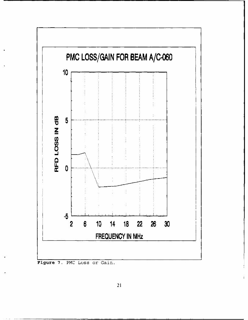
c. Primary Multicouplers (PMC)
Primary multicoupler loss or gain is measured by the same technique
used to measure the ENLARGER loss. A graph of PMC loss and gain is shown in
Figure 7.
2. Excess Noise Floor
Excess noise produced by components within the RFD system may increase
the noise floor over that of the primary multicouplers. The reference noise floor limit
for the receiving systems was set at -125 dBm for a 3 kHz gaussian-shaped bandwidth.
This is approximately the noise floor of the type 1382 multicouplers used as the PMCs.
It is also close to the noise floor of several receiving systems used in CDAA sites. If
the RFD system produces noise levels in excess of the reference limit, then low-level
signals will be undetectable because they are below the RFD noise floor. The difference
between the reference floor limit and the RFD measurements is the excess noise floor.
A graph of the excess noise floor versus frequency is shown in Figure 8.
The noise floor ic measured (see Figure 3) with all inputs to the appropriate
beam terminated. This eliminates all externally generated noise and avoids the problem
of separating external from internal noise. The primary source of excessive noise in the
RFD is the active elements within ENLARGER [Ref. 6:p. 25].
3. Internal Sources of Man-Made Noise
The introduction of inadequately and improperly shielded electronic equipment
within the CDAA sites has resulted in an internal noise problem at most locations.
20
PMC LOSS/GAIN FOR BEAM A/C-060
10
0
0
-5
2 6 10 14 182226 30
FREQUENCY IN MHz
Figure 7. PMC Loss or Gain.
21

EXCESS NOISE FLOOR FOR BEAM A/C-060
15
Z 1 .. .. ... ... ......................................... ...................................10 -
0
W "05
2 6 10 14 18 22 26 30
FREQUENCY IN MHz
Figure 8. Excess Noise Floor.
22
Internal electronic devices such as mini-computers, workstations, PC's, LAN's,
uninterruptible power supplies (UPS), frequency converters, digital telephone switches,
and other digital equipment generate radio interference. The noise from such devices is
conducted along power wires, ground buses, cable shields, air-conditioning ducts, and
other conductors. It enters the RFD by a variety of paths and is in turn fed to the input
terminals of receivers.
The measurement, identification, and location of specific internal noise sources
is a long and tedious process. The most effective method of locating internal sources is
to monitor the waveform (temporal and spectral structure) of each suspected internal
noise source and then physically search for sources that can generate these structures.
For example, by correlation with an on/off light switch, a faulty fluorescent light ballast
close to an antenna cable bundle may be positively identified as the source of HF noise
observed on the 3-axis display (see Appendix B). This process, often involving trial and
error, may require many man-days of effort, especially if the source is intermittent. If
the source is not physically located and eliminated, then its noise interference contributes
to the noise floor used in the PET evaluation. Equipment currently used to identify and
record the noise or interference source waveforms is described in Appendix B. The
waveforms obtained with the 3-axis display for internal sources are often similar to those
for external sources.
4. External Sources of Man-Made Noise
Sources of noise external to the site are an ever-increasing problem as the
development of land in close proximity to the site is constantly taking place. Power-line
23
noise is the most prevalent of all external noise sources [Ref. 7:p. 17]. A photograph
of the 3-axis display waveform (temporal and spectral structure) for power-line noise is
shown in Figure 9. All signals within the 2.6 to 4.0 MHz band and having a smaller
signal strength will be lost to the noise interference. The masking of the weaker signals
by another case of power-line noise is shown in Figure 10. The temporal and spectral
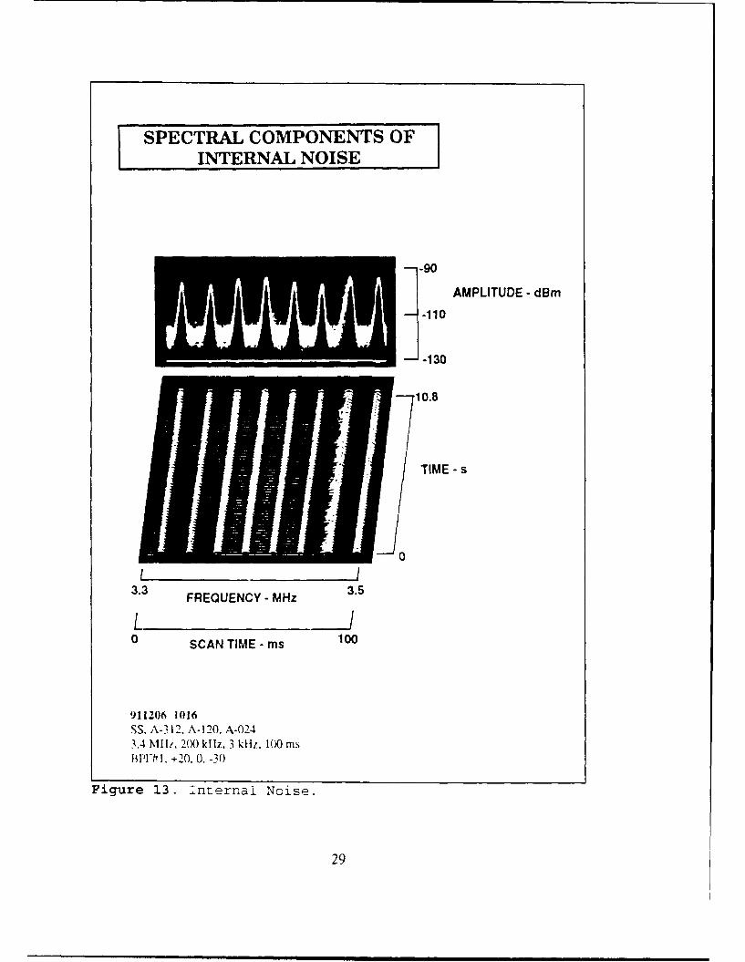
structure of ignition noise is shown in Figure 11. This source is external to the site. A
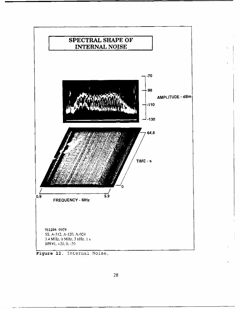
view of the gross spectral structure of a specific kind of internal noise is shown in Figure
12. Figure 13 shows the distinctive fine temporal and spectral shape of the internal noise
of Figure 12.
Out-of-band emanations from equipment in the Industrial, Scientific, and
Medical (ISM) radio service causes large numbers of SOIs to be lost in some receiving
systems [Ref. 8:pp. 76-79]. The intermittent nature of out-of-band ISM signals makes
their identification difficult unless wide-band monitoring systems are available. Even
when identification and location is possible, it may not be feasible to correct all ISM
problems. This is especially true for distant ISM sources located in other countries.
Such signals may traverse one or two ionospheric propagation hops before arriving at a
receiving site.
The spectral and temporal characteristics of all man-made noise, from both
internal and external sources, must be measured and recorded for use in the performance
evaluation. The percentage of signals lost due to man-made sources is often significant.
24

POWER LINE NOISE
-60
_80
AMPLITUDE -dBm
-- 100
-J-120
TIME -s
-A0
2.4 FREQUENCY - MHz 4.
0 SCAN TIME -ms 100
911205 1534SS, A-0363.4 Mlz. 2 MHz, 30 kliz, 100 msBPF# 1, +20. 0. .20
Figure 9. Power Line Noise.
25

POWER LINE NOISE
-50
POWER-LINE NOISE-7AMPLITUDE -dBm
-90
LOW-LEVEL SIGNALS -_110
1.5 FREQUENCY - MHz 6.5
0 SCAN TIME -ms 200
911204 0930SS. A- 1804 MHz. 5 M11z. 30 kl-Iz, 200 msBPF#6, +20, 0 -10
Figure 10. Power Line Noise Hiding Signals.
26

IGNITION NOISE
-- 60
-- 80
AMPLITUDE -d~m
-- 100
-J-120
10.8
U TIME - s
0
0 100SCAN TIME - ms at 4 MHz
911204 1003SS, A-2884 M-z, 0MN11. 30 kiU. Il() is (LS)BPFr#I. +20. o, -20)
Figure 11. ignition Noise.
27
SPECTRAL SHAPE OFINTERNAL NOISE
-- 70
-90
AMPLITUDE dBm-E1p0h~hi130
64.8
FREQUENCY - MHz
911206 0j959SS. A-3 12. A-120, A-0243.4 MlHz. 0 Mliz. 3 kHz. 1 sB PF# 1,-.20. 0, -3 0
Figure 12. internal Noise.
28
SPECTRAL COMPONENTS OFINTERNAL NOISE
-- 90] AMPLITUDE - dBm
-110
, -130
10.8
TIME - s
FREQUENCY - MHz
L /0 SCAN TIME - ms 100
911206 1016SS. A-312, A-120. A-0243.4 M lz, 200 kihz. 3 kliz, 100 msHPI-f 1, +20, 0. -30
Figure 13. Internal Noise.
29

5. International Broadcast Service Interference
The HF band contains a number of sub-bands allocated to the International
Broadcast Service. Transmitters in this service frequently employ power levels of 1 MW
or higher and antennas with gains approaching 20 dB. These transmitters produce
extremely strong signal levels at CDAA sites. The signals may be as high as 40 to 50
dB above the maximum levels of most SOIs. The mix of very strong signals from
transmitters in the International Broadcast Band and low-level SOIs requires that RFD
components have very high dynamic range (more than 100 dB).
RFD components with insufficient dynamic range to handle the large
amplitude range of received signals will generate intermodulation (IM) products. These
IM products also degrade the performance of CDAA or other receiving sites. The
impact of IM products on site performance is not the primary topic of this thesis. and the
adverse impact of this aspect of site operation is not covered.
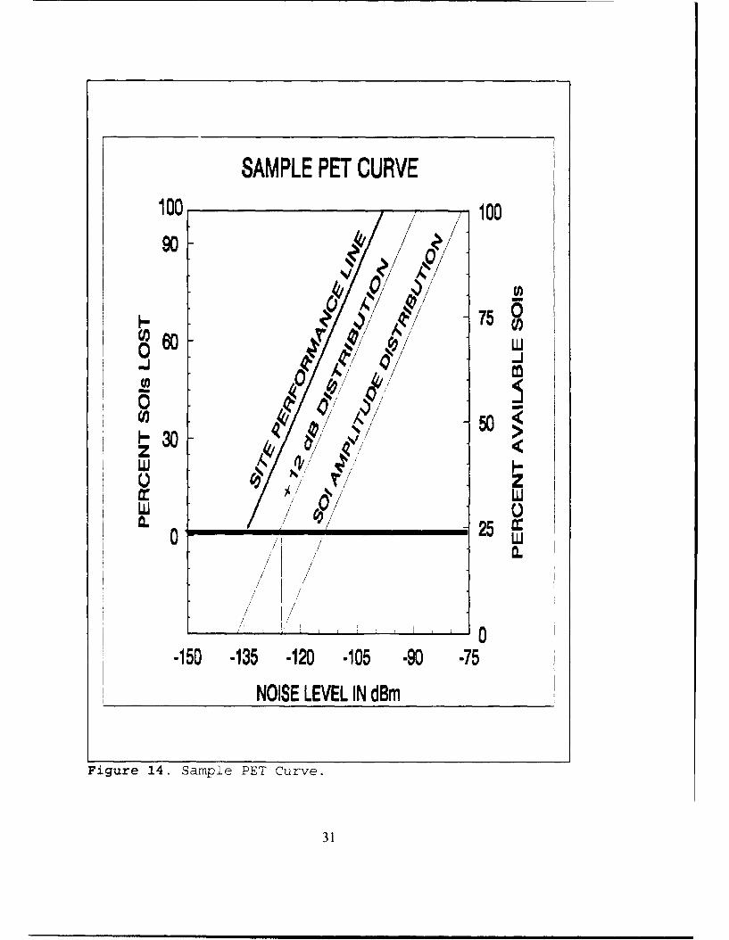
E. THE PET CURVE
The PET curve has been developed to quantify and measure the effects of system
degradation on the reception of SOIs. It combines the diverse factors of signal strength.
noise floor, RFD loss, and man-made noise into a meaningful graphical relationship. By
using the PET graph and varying the input parameters, the performance of a receiver
system can be measured by determining the percent of SOIs lost. A complete PET curve
sample is shown in Figure 14. The steps for the construction and interpretation of the
curve are as follows.
30
SAMPLE PET CURVE100 100
900
7506 0 0)
-J -J
S 40/
/, ~ ~/
30
z / "/ /
o z
/ /
/,/
*1' 0-150 -135 -120 -105 -90 -75
NOISE LEVEL IN dBm
Figure 14. Sample PET Curve.
31

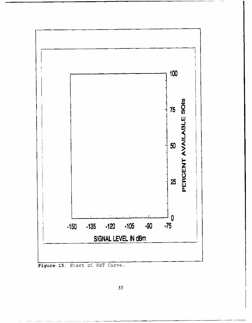
1. Construction
The PET curve construction process begins with a two dimensional x-y plot
as shown in Figure 15. The x-axis represents the signal power in dBm of SOIs received
by a site's antenna system. The y-axis is located to the right, vice the normal convention
of location on :he left. This will allow for the subsequent addition of a second y-axis.
The y-axis scale rerresents the percent of available SOIs that exceed the received power
level shown on the x-axis. The resulting curve is the amplitude distribution of a selected
class SOIs.
a. SOI Amplitude Distribution
A straight-line approximation of the SOI Amplitude Distribution is
sufficiently accurate for general PET use. The procedure for generating this
approximation follows.
Enter a point on the x-axis at the noise floor level of -125 dBm and the
y-axis value of 0 percent. This point is the left end of the distribution. The second point
of the straight-line approximation is the x-axis value of the maximum signal strength
expected, in dBm, and the y-axis value of 100 percent. Connect the two points with a
straight line. This line will represent the straight-line approximation of the SO
Amplitude Distribution.
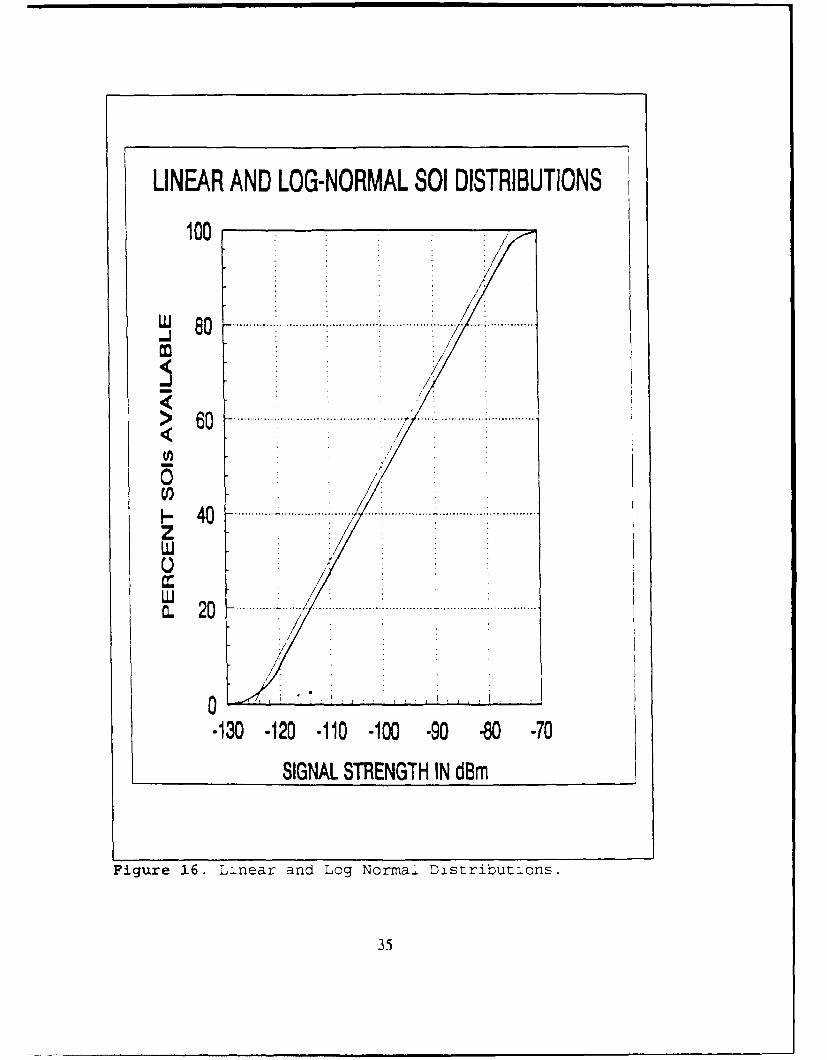
The amplitude distribution of SOIs is more accurately shown by a log-
normal distribution. An illustration of the straight-line approximation superimposed over
32
100
7580-J
5
25
0.
-150 -135 -120 -105 -90 -75
SIGNAL LEVEL IN dBm
Figure 1s. Start ofi PET Curve.
33

a log-normal distribution is shown in Figure 16. The primary differences are at the
extreme ends of the distribution.
Appendix D presents data confirming the log-normal amplitude
distribution of certain classes of SOIs [Ref. 3:pp. 28-451. While the log-normal
distribution can be used in the PET process, the minor error generated by the straight-
line approximation does not greatly affect the final results.
To understand the use of the linear approximation of the SOI Amplitude
Distribution, consider the following example. In Figure 17, enter the x-axis with a signal
level of -95 dBm, the intersection of this level with the distribution line will yield a
corresponding value of SOIs available on the y-axis. Sixty-four percent of the total SOIs
are below this level and 36 percent of the total SOIs are above this level.
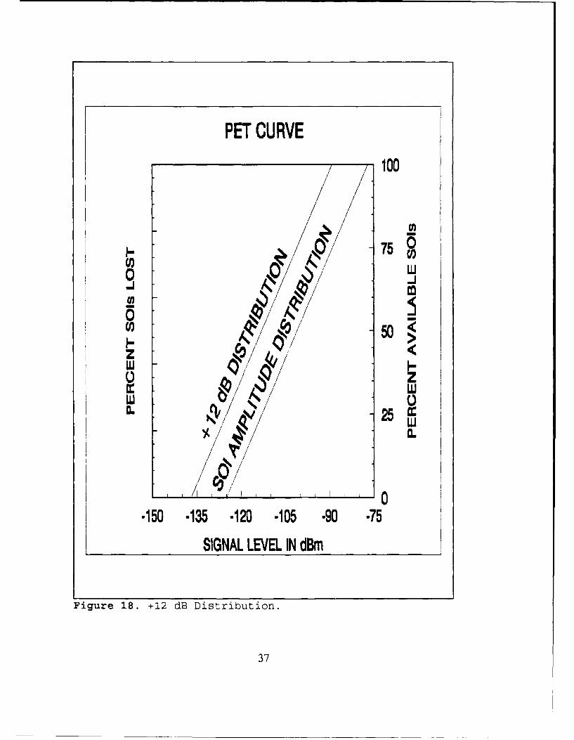
b. +12 dB Distribution
A + 12 dB Distribution line is drawn parallel and to the left of the SOI
Amplitude Distribution. This line represents the amplitude distribution of SOIs that are
12 dB above the receiver noise floor. This is approximately the signal-to-noise ratio
required for the detection and processing of SOIs by conventional digital signal
processing techniques. All procedures from this point on will be based on the + 12 dB
Distribution and the left y-axis. Figure 18 shows the + 12 dB Distribution line.
c. Percent SOIs Lost
A second y-axis scale located on the left of the curve will be constructed
using the following steps. Enter the x-axis at the reference noise floor limit, in this case
34
LINEAR AND LOG-NORMAL SOl DISTRIBUTIONS
100
0zLU
LU .. - ............... -. . .
-130 -120 *110 -100 -90 -80 -70
SIGNAL STRENGTH IN d~m
Figure 16. Linear and Log Normal Distributlons.
35

PET CURVE
*100
7/ 75
ge 64O 50<
LU
0.
-95 dBmC3 1 +I I 0
-150 -135 -120 -105 -90 -75
SIGNAL LEVEL IN dBm
Figure 17. Amplitude Distribution Example.
36
PET CURVE
100
750_, w
0 k-
U , "50
S/ . , <
25
0.
-150 -135 -120 -105 -90 -75
SIGNAL LEVEL IN dBm
Figure 18. +12 dB Distribution.
37

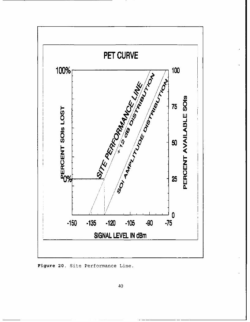
-125 dBm. Proceed up to the + 12 dB Distribution line. Where -125 dBm intersects the
line, proceed left and mark the y-axis 0 as shown in Figure 19. This marks the base
value of percent of SOIs lost. The top point of the y-axis will be 100, with the axis
scaled accordingly. The graph now represents the optimum performance of a receiving
system. The operating point where -125 dBm intersects with the +12 dB distribution
corresponds to a 0 percent signals lost. With no RFD loss introduced into the curves,
the + 12 dB Distribution line, shown in Figure 20, is the Site Performance line.
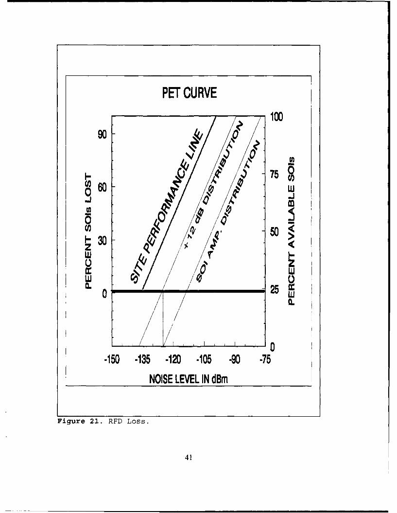
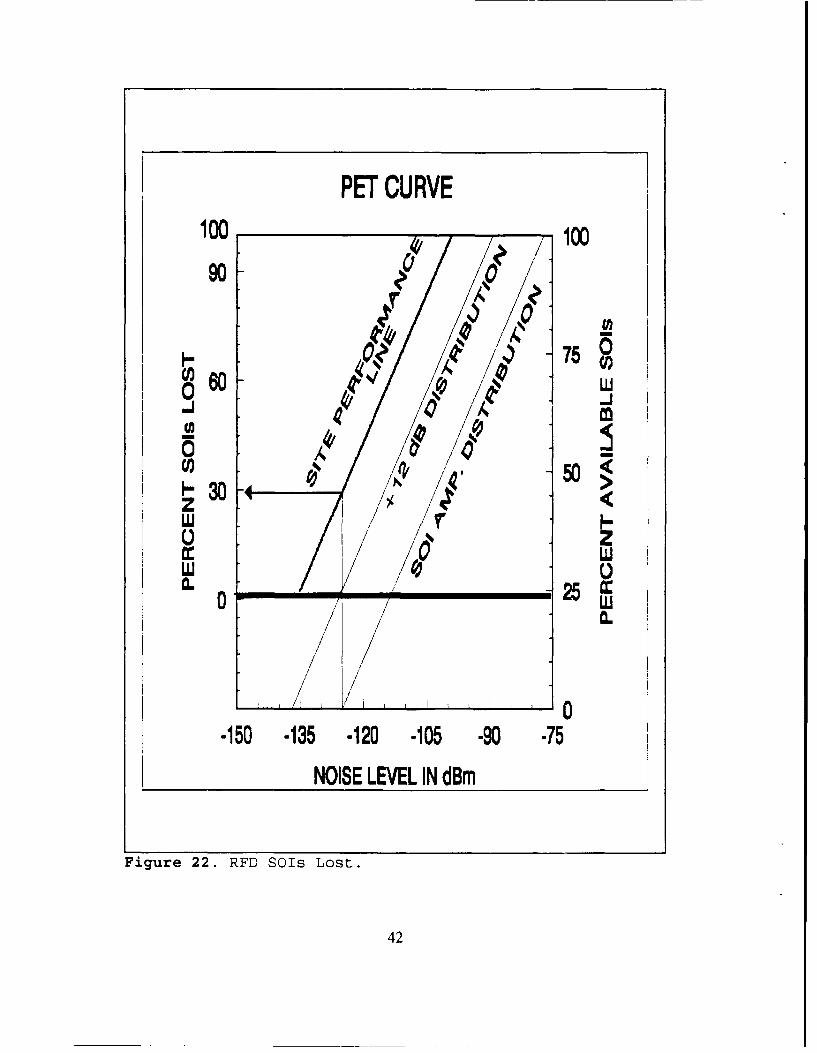
d. Performance With RFD Loss Added
The curve from Figure 20 will now be revised to include the effect of
the signal attenuation within the RFD. The sum of the attenuations of all components
in the RFD at a particular frequency is added to the Site Performance line. This moves
the line to the left as shown in Figure 21. The new performance line represents the
optimum performance the site can attain with the RFD loss introduced. The intersection
of the -125 dBm level with the Site Performance line produces the percent of SOIs lost
due to signal attenuation in the RFD as shown in Figure 22.
e. Performance With Excess Noise Floor Added
The impact of an increase in system noise over the reference noise floor
is illustrated as follows. Enter the actual noise floor of the RFD (-125 dBm plus excess
noise level) into the x-axis for the corresponding frequency of operation. Signals that
are above -125 dBm but still below the excess noise floor are now lost. The new
operating point is the intersection of the excess noise floor with the Site Performance line
38

PET CURVE1 ,/ 100
'/
7580 J
W, 50<
z
/ N,o 4'0 2/ 125dBm
/, -
-150 -135 -120 -105 -90 -75
SIGNAL LEVEL IN dBm
Figure 19. o SOIs Lost.
39
PET CURVE100% 100
k 0
7 0
05
SINA LEEN d4m
z4O
~1 25/W
* 150 -135 -120 -105 -90 -75
SIGNAL LEVEL IN dBm
Figure 20. Site Performance Line.
40
PET CURVE100
& 750-JJ
~30 <zz
0 /f' 250 L0
150 135 120 -105 -90 -75NOISE LEVEL IN dBm
Figure 21. RFD Loss.
41
PET CURVE100. 10090 0
T 0
-150 -135 -120 -105 -90 75
0 w LU
4250~30 0 4
zz
w /0
.10 -135 -120 -105 -90 -75
Figure 22. RED SO~s Lost.
42

as shown in Figure 23. The intersection of the excess noise floor with the Site
Performance line yields the percent of SOIs lost on the y-axis, due to both RFD
attenuation and excess noise floor. Figure 24 shows percent of SOIs lost due solely to
RFD attenuation and RFD noise floor at one particular frequency. Excess noise floor
over the entire HF band is defined in Section 1.D.2.
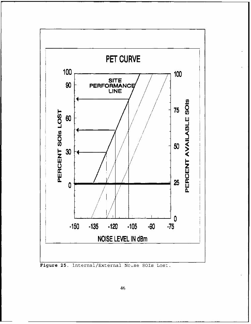
f. Performance With Internal or External Noise Added
The PET curve can be further modified to assess the impact of internal
and external man-made noise that is received by the system. Enter the amplittude le\"el
of man-made noise into the x-axis for a selected frequency. The point at which this level
intersects with the Site Performance line represents the new operating point for the
presence of noise. Where this point intersects with the y-axis yields the percent of SOIs
lost due to man-made noise, excess noise floor, and RFD loss. Figure 25 shows an
example of the impact of an internal or external noise level of -107 dBm on the
performance curve.
2. Interpretation of PET Curve Results
This section provides a more comprehensive description of the effects of RFD
noise, excess noise floor, and noise levels on site performance. It provides additional
examples of site degradation with the corresponding changes on percent SOIs lost. The
optimum performance curve shown in Figure 20 and reproduced in Figure 26, will be
the basis from which to start the examples.
43

PET CURVE100 10090 ci 10
0% 4 4 750
0 0
0 15 -13 .10 15 -
4
U,4, 50~z
'I za: W
- 25
0.
-150 -135 -120 *105 -90 -75
NOISE LEVE IN dBm
Figure 23. Excess Noise Floor SOIs Lost.
44

PET CURVE100
00
"0 k 75:
"0 -A 0
o, W
U' 50<-30z <
LUU
w / 0
0. _ _ _ 25 L
', ; , I / 0 .
0-150 -135 -120 -105 -90 -75
NOISE LEVEL IN dBm
Figure 24. Total SOIs Lost.
45
PET CURVE100 100
SITE90 PERFORMANC
LINE
75
ww
z z
a: LU/ I-
U0b i 25 W
/
/~ 0
-150 -135 -120 -105 -90 -75
NOISE LEVEL IN dBm
Figure 25. Internal/External Nc±se SOIs Lost.
46

PET CURVE100 100
910Aa
75 0
owJ J
k00,, o
z <
w 0C.__ __ _ 250 wU
/0.
-150 -135 -120 -105 -90 -75
NOISE LEVEL IN dFP
Figure 26. Optimum PET Curve.
47
RFD loss moves the site performance curve left by the amount of the loss.
Since the optimum operating point for the system is where the reference noise floor
intersects the Site SOI Performance line, the added RFD noise produces a corresponding
percentage of SOIs lost. Figures 27-29 show examples of RFD loss in dB steps and the
corresponding percent of SOIs lost. One can plainly see that the best performance
attained is when there is no RFD loss and the Site SOI Performance line is the same as
the + 12 dB amplitude distribution.
The impact of excess noise floor on the reception of SOIs is determined by
entering the excess noise into the x-axis and establishing a new operating point on the
Site Performance line. Figure 30 shows the effect of an excess noise floor of 6 dB. The
percent of SOIs lost due to the changing noise floor to an excess of 8 dB is shown in
Figure 31. The system can perform best when there is no excess noise floor and the
reference noise floor sets the operating point.
The presence of internal and external man-made noise also degrades site
performance. The noise amplitude can vary with frequency and bearing, and the
examples address both factors. The man-made noise level is entered on the x-axis. The
point where the noise level intercepts the Site Performance line is determined and the
resulting loss in SOI reception is established. The effect here is the same as an excess
noise floor level. The presence of man-made noise masks or hides the signals of weaker
strength. Figure 32 shows another example of the spectral shape of power-line noise.
All the signals below the level of the power-line noise are effectively hidden in the noise
and cannot be detected because of the noise. The photograph is scaled to the settings of
48

PET CURVE100 100
75 060 - "0-J 0
30z<WU 0~
/t/
/ / 25x
/ /
0-150 -135 -120 -105 -90 -75
NOISE LEVEL IN dBm
Figure 27. 6 dB RFD Loss, SOIs Lost.
49

PET CURVE10010
90 !
/v
7 0
-0 0 -5
0U 0
LU 00. __ _ __ _ _ _ 25
0 //I /U
0.
-150 -135 -120 -105 -90 -75NOISE LEVEL IN dBm
Figure 28. 8 dB RFD Loss, SOIs Lost.
50

PET CURVE100 /1 100
90 ///75
o 0 0 V-J 40 -
05
/ /o z
/ W
0 /
0./ , /
-150 -135 -120 -105 -90 -75
NOISE LEVEL IN dBm
Figure 29. 12 dB RFD Loss, SOIs Lost.
51

PET CURVE100 ,100
90 4 /
750K0 40-0
U, / 50<-30 -z<
() /
/ 0
0 < dB NOISE ECESS
// t
-150 -135 -120 -105 -90 -75NOISE LEVEL IN dBm
Figure 30. 6 dB Excess Noise Floor, SOIs Lost.
52

PET CURVE100 100
~60
//
/ 5075
0 25
4/ 8 dB NOISE EXCESS./
/ j /
0-150 -135 -120 -105 -90 -75
NOISE LEVEL IN dBm
Figure 31. 8 dB Excess Noise Floor, SOIs Lost.
53

POWER LINE NOISE
-60
-80o
AMPLITUDE
-- 100 dBm
-120
2.5 FREQUENCY - MHz 7.
0 SCAN TIME -ms 20
911203 1050SS, A-2405 MHz. 5.%MHz. 10 kl~z, 20 ms (LS)LPF#[. +20, .10.-20
Figure 32. Power-Line Noise.
54

the measurement equipment. The amplitude of the noise at the PET curve frequency is
entered into the graph. Figure 33 shows an example of SOIs lost due to two man-made
sources that produce noise at levels of -101 dBm and -110 dBm. This represents SOIs
lost of 68 and 45 percent, respectively.
3. Site Performance Evaluation
The impact of all the different factors degrading overall performance of a site
at a particular frequency, bearing, and time of day can be assessed. A full survey would
encompass all frequencies in the 2-30 MiHz HF band, all beams of coverage, and a 24
hour day. The percent of SOIs lost can be compiled for each condition and an overall
result can be produced, as shown in Figure 34. The data graphed in this figure
summarizes variations in performance over the 2-30 lMHz band of frequencies,
corresponding to 4-hour increments, throughout one day. This particular summary shows
the impact of site-related factors, but it does not show the impact of man-made noise.
Additional examples are required for a full evaluation of site performance.
55

PET CURVE100 /100
SITE /PERFORMANCE
LINE 7II.- 4758
~60 wU-Jo 7 o
So0 / ,503/ .w <-
LUL0 wU
I ; 5"0 -101
-150 0
150 -135 -120 -105 -90 -75
NOISE LEVEL IN dBm
Figure 33. Internal/External Noise, SOIs Lost.
56

24 HOUR SOls LOSTDUE TO RFD LOSS AND EXCESS NOISE FLOOR0-w
70 '00+0400*::BEAM* . A/C-060 -20
-12000, *2000
~0..............
U) 5 ... ........... ..... .. .. .
30 I
2 6 10 1418 2226 30FREQUENCY IN MHz
Figure 34. Overall SOIs Lost.
57

IV. AUTOMATED PERFORMANCE EVALUATION TECHNIQUE
The manual manipulation of the large amount of data needed for a comprehensive
performance evaluation of CDAA sites has been a challenge to the SNEP teams. This
chapter outlines the steps required to use a personal computer to perform a PET analysis
on a site and its receiving systems. A commercially available software package, 3-D
Visions GRAFTOOL, was selected based on its flexibility. The next step in refining the
automated PET requires that a custom software program be written to perform the
analysis. This step is not addressed here other than as a recommendation. The
remainder of this thesis describes the procedures for the implementation of the PET on
an IBM compatible computer using GRAFTOOL.
A. GRAFTOOL, SCIENTIFIC ANALYSIS PROGRAM
GRAFTOOL is a commercially available scientific software package used to
analyze and present data [Ref. 9:p. 3]. The application of the PET using GRAFTOOL
eliminates the tedious work of manipulating large amounts of data with pencil and paper.
All computational and line-intercept work is performed within the program and is faster
and more accurate than achievable with the previous manual methods.
Certain conventions for file naming and data reference were developed to ensure
standardization and interoperability. Presentation of the results is in the standard PET
format, using percent of SOIs lost as the operating performance measure.
58

A working knowledge of GRAFTOOL must be attained before using the automated
PET. The program is totally menu-driven. Review time should be dedicated to learning
the program before attempting to use the automated PET. All of the following sections
are presented assuming a working knowledge of the program.
B. FILE MANAGEMENT AND DATA INPUT
All the data files have the extension .DAT. Contained in the files are the points
needed to construct the SOI Amplitude Distribution, + 12 dB Distribution, and Site SOI
Performance lines. The files also contain values representing the percent SOIs lost as
a function of frequency and time of day. The data-file naming convention for line
distributions is XXTFFMQ.DAT. "XX" represents the hour of the day using the 24
hour clock. For example, data is evaluated at 4-hour increments, therefore, the values
for XX are 00, 04, 08, 12, 16, and 20. "T" is for time. "FF" denotes the frequency
of operation in MHz. The range will be from 2-30 MHz in 2 MHz increments, where
"M" to represent lHz. "Q" is the number of the file, ranging from 0-4, and represents
the different data set that it contains. File 0 contains two points corresponding to the
values of the reference noise floor and the maximum signal strength expected at the
designated time and frequency. File I is the linear regression of file 0 and contains all
the points that make up the SO1 Amplitude Distribution line. File 2 contains the points
of the + 12 dB Distribution line. File 3 contains the two points defining the site line, and
file 4 is the linear regression of the site line. A summary list of all file names is listed
below. The remaining files in the list will be covered as the topics are discussed.
59

* XXTFFMQ.DAT where XX = 00-20, FF = 2-30, Q = 0-4.
* XXSILSTQ.DAT where XX = 00-20, Q = 1-4.
To illustrate the data-file naming, the following examples are presented.
06T10M2.DAT indicates the data file containing the information for the time 0600 and
operating frequency of 10 MHz. Data file 2 represents the data points for the + 12 dB
Distribution line. 12T30M4.DAT is time 1200, frequency 30 MHz and the file
containing the regression points that make up the Site SOI Performance line. When the
final graphs are constructed, the data files used are the XXTFFM1.DAT,
XXTFFM2.DAT and XXTFFM4.DAT.
When the percent of SOIs lost is extracted from the curves, the values are stored
in files for processing. Since the percent SOIs lost corresponds to a specific time of day,
but varies with frequency, the naming convention for these files is XXSILSTQ.DAT.
"XX" is the hour of day on the 24 hour clock and "SILST" represents SOIs lost. "Q"
is the file number with I used for the percent SOIs lost due to the RFD, file 2 holds the
loss from the RFD plus excess noise floor, file 3 is the loss from internal and external
noise with RFD loss and file 4 is the combination of the maximum loss of files 1-3.
C. CREATING PET CURVES
This section details setting up the curves prior to data entry. All commands entered
into the computer are written in capital letters. Figures showing the screen output are
provided as needed.
60
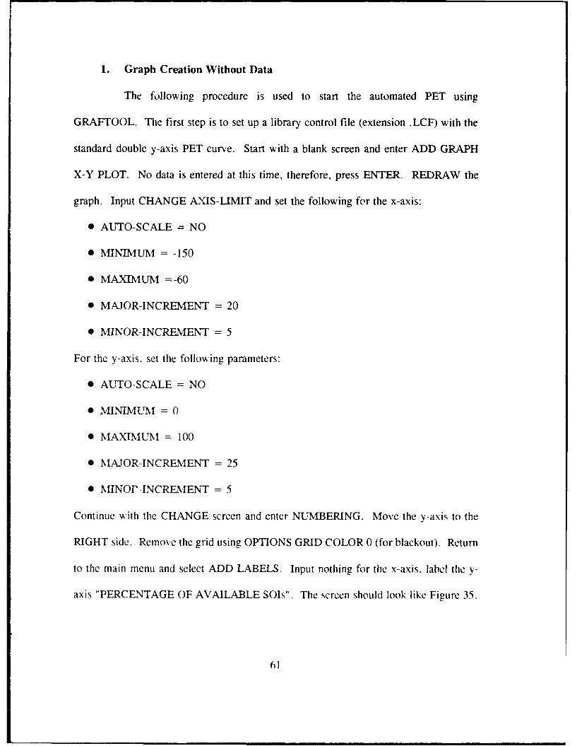
1. Graph Creation Without Data
The following procedure is used to start the automated PET using
GRAFTOOL. The first step is to set up a library control file (extension .LCF) with the
standard double y-axis PET curve. Start with a blank screen and enter ADD GRAPH
X-Y PLOT. No data is entered at this time, therefore, press ENTER. REDRAW the
graph. Input CHANGE AXIS-LIMIT and set the following for the x-axis:
* AUTO-SCALE = NO
* MINIMUM = - 150
* MAXIMUM =-60
* MAJOR-INCREMENT = 20
" MINOR-INCREMENT = 5
For the y-axis, set the following parameters:
" AUTO-SCALE = NO
* MINTIMUM = 0
* MAXIMUM = 100
* MAJOR-INCREMENT = 25
" MINOP-INCREAIENT = 5
Continue with the CHANGE screen and enter NUMBERING. Move the y-axis to the
RIGHT side. Remove the grid using OPTIONS GRID COLOR 0 (for blackout). Return
to the main menu and select ADD LABELS. Input nothing for the x-axis. label the y-
axis "PERCENTAGE OF AVAILABLE SOIs". The screen should look like Figure 35.
61

100
75 .1
0
0
25 z~
0.
-150 -130 -110 -90 -70
Figure 35. Axis to Start PET.
62

Select LIBRARY and enter the name SOIDIST.LCF, representing SOI Distribution. The
graph is saved as a template without data.
A second graph will be overlaid on the first template. Start with a clear
screen and select ADD GRAPH X-Y PLOT. No data is required, so press ENTER.
Select CHANGE AXIS-LIMIT and change the x-axis to the same set up as the
SOIDIST.LCF template. Set the y-axis as follows:
* AUTO-SCALE = NO
* MINIMUM =-25
* MAXIMUM = 100
* MAJOR-INCREMENT = 25
* MINOR-INCREMENT = 5
Go to the NUMBERING command and SUPPRESS the first number (-25) on the y-axis.
Select LABELS. name the x-axis "NOISE LEVEL IN dB" and the y-axis "PERCENT
SOIs LOST". The graph should look like Figure 36. Return to the main menu and
select LIBRARY. Enter the name SITEDIST.LCF. representing Site Distribution. for
this graph. These two graphs will be used for all the other cunes with only minor
modifications.
2. Signal Strength Data Entry
The data points for the SO1 Amplitude Distribution are entered into the
GRAFTOOL worksheet. The extension on the file is .DAT and uses the naming
convention from section B. From the main menu select WORKSHEET. Enter the
reference noise floor level in cell Al. Enter the maximum signal strength expected in
63

100 .. 100
75 w75i
U)02
Jw500
5
0
CL 0
-150 -130 -110 -9 -70
NOISE LEVEL IN dB
Figure 36. Two Axis PET Curve.
64
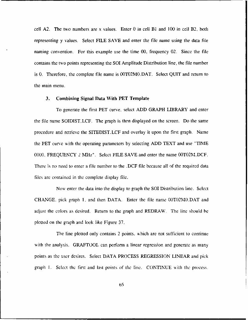
cell A2. The two numbers are x values. Enter 0 in cell BI and 100 in cell B2. both
representing y values. Select FILE SAVE and enter the file name using the data file
naming convention. For this example use the time 00, frequency 02. Since the file
contains the two points representing the SOI Amplitude Distribution line, the file number
is 0. Therefore, the complete file name is OOT02MO.DAT. Select QUIT and return to
the main menu.
3. Combining Signal Data With PET Template
To generate the first PET curve, select ADD GRAPH LIBRARY and enter
the file name SOIDIST.LCF. The graph is then displayed on the screen. Do the same
procedure and retrieve the SITEDIST.LCF and overlay it upon the first graph. Name
the PET curve with the operating parameters by selecting ADD TEXT and use "TIME
0000. FREQUENCY 2 MHz". Select FILE SAVE and enter the name OOT02M.DCF.
There is no need to enter a file number to the .DCF file because all of the required data
files are contained in the complete display file.
Now enter the data into the display to graph the SOI Distribution line. Select
CHANGE, pick graph 1. and then DATA. Enter the file name OOT02MO.DAT and
adjust the colors as desired. Return to the graph and REDRAW. The line should be
plotted on the graph and look like Figure 37.
The line plotted only contains 2 points, which are not sufficient to continue
with the analysis. GRAFTOOL can perform a linear regression and generate as many
points as the user desires. Select DATA PROCESS REGRESSION LINEAR and pick
graph 1. Select the first and last points of the line. CONTINUE with the process.
65

PET CURVE TIME 0000, FREQUENCY 2 MHz100 100
* 0755E
0
U) <
zz
L 25wZL0... ....... ..... C
-150 *130 -110 -90 -70
NOISE LEVEL IN dB
Figure 37. PET Curve With SOT Distribution.
66

Output the data to file name OOT02M1 .DAT. All the data points from the line regression
are placed into data file 1. REPLACE the data file 0 with data file 1 in the graph.
The next data file will be the + 12 dB Distribution line. Select WORKSHEET
BLANK and from the menu select FILE MERGE. The cell location to merge with is
El. The file name is OOT02M1 .DAT. All the data points are loaded into columns E and
F. The + 12 dB Distribution line is a line parallel to the SO1 Amplitude Distribution and
thus will have the same slope, but moved 12 dB to the left. Return to column A, select
DATA INITIALIZE FORMULA and choose the range Al..Al00. Enter the formula
$El-12. Column A now has all the new x-axis values for the + 12 dB line. COPY the
y-axis values from column F, to column B. to complete the data points. FILE SAVE
and name the data file 00T02M2.DAT, as per the file naming convention. Return to the
main menu with the OOT02M.DCF file on the screen.
Enter the + 12 dB Distribution line data into the SOIDIST graph of the
display. Select CHANGE. pick graph 1, DATA and select F8 for a second data file in
the same graph. Enter the data file name 00T02M2.DAT and return to the graph.
REDRAW and the screen should resemble Figure 38.
The site performance line will have the same slope as the + 12 dB line and
when there is no loss. the two lines lie on top of one another. The difference in the lines
is the y-axis values for the corresponding points on the x-axis. Since the reference noise
floor intersection of the + 12 dB line sets the 0 percent SOIs lost, the data is plotted in
the second graph. Select DATA EXTRACT and pick the + 12 dB line. The first point
is located where the x-axis value is as close to the value of the reference noise floor as
6-7

PET CURVE TIME 0000, FREQUENCY 2 MHz
100 100
05 ................... . ................ •..... ,.......... ? ....... .. ........ ! ....... <U75 / (1
" .s .................................... ........ ....... .... ...
/ 500
z ~, / .. ..../ / ......2.. .........I ..... 5//.
Lu 5 ............... . .'
c/ <
I UL
//
/ /
/25 z~0 . .... . ...... ...... ;l... .......... .......... I.....
/ 0I , , , I 0
-150 -130 -110 -90 -70
NOISE LEVEL IN dB
Figure 38. PET Curve With +12 dB and SOI Distributions.
68

possible. In this case it should be close to -125 dBm. The last point selected is where
the y-axis value is 100. The file name for the data extraction is 00T02M3.DAT.
From the main menu select WORKSHEET BLANK and then FILE LOAD
with the file 00T02M3.DAT. The file contains all the points of the line from the noise
floor to the maximum signal strength less 12 dB. The data must be edited before
returning it to the graph. The value in cell Al should be edited to -125 dBm. Change
cell BI to 0. Delete the range from 2-99 and move the last data point to A2 and B2.
The file should have only two data points remaining. The first point, in row 1, has the
value of -125 and 0. The numbers located in row 2 should be the new maximum signal
strength value and 100. Save the edits, the file, and return to the 00T02M.DCF display.
The next step is to enter the Site Performance line into graph 2 of the display.
Select CHANGE, pick graph 2 this time, and select DATA. Enter the data file name
00T02M3.DAT into the graph and edit the colors as necessary. Return to the display
and REDRAW. The Site Performance line will lie over the + 12 dB line because there
is no loss added as yet. However, the Site Performance line will only extend to 0
percent SOIs lost as the line has no meaning below 0.
The final step in completing the data files is to develop more points for the
Site SOI Performance line by using the linear regression process again. From the main
menu, select DATA, pick graph 2, enter the first and last points and complete the
regression. Send the data to file 00T02M4.DAT and replace file 3 with file 4. Redraw
the complete graph. the Site Performance line is on top of the + 12 dB line because there
is no loss.
69
The final result is a display file OOT02M.DCF consisting of 2 graphs overlaid
upon each other with data files OOT02M1.DAT, 00T02M2.DAT in graph 1 and
00T02M4.DAT in graph 2. No loss is entered into the plot of the site line, therefore it
is located over top of the + 12 dB line.
4. Site Performance Curve With RFD Loss
The loss due to the RFD must now be added to the Site SOI Performance line.
The loss is frequency dependent, therefore a plot of RFD loss versus frequency is
required so that the loss value can be put into the data file 00T02M4.DAT.
Enter the RFD loss curve at 2 MHz. The corresponding loss data is added
to the x-axis data in the file. From the main menu, select WORKSHEET BLANK and
FILE MERGE 00T02M4.DAT into columns E and F. In the cell Cl enter the loss data.
Select DATA INITIALIZE FORMULA and choose the range A1..A1OO. Enter the
formula SEI-SCSI. The values in column A are now the site points with the RFD loss
added. The loss value may be edited at any time to do "what if" calculations if the loss
is reduced. COPY column F to column B. Return to the OOT02M.DCF display graph.
REDRAW the graph. and the site line has now moved to the left showing the effect of
the loss and should look like Figure 39.
5. PET Curves With Excess Noise Floor
The PET curve with RFD loss is shown in Figure 39. Tile next step is to add
the effects of moving the reference noise floor to the right by the amount of the excess
noise. Start with the 00T02M.DCF display file. Add to the reference noise floor the
70

PET CURVE TIME 0000, FREQUENCY 2 MHz
100 . 100
075 ................................ ............... ..... ;.....
75
50 50
ui25 w': /0
/ /// z
L 25 . ... . . I........ .............
I0
',-150 -130 -110 .90 -70 0NOISE LEVEL IN dB
Figure 39. PET Curve With Site Performance, +12 dB and SOTDistribution.
71

amount of excess noise and mark the x-axis at the corresponding point with an arrow.
Select ADD ARROW from the main menu and draw the arrow up to the intersection
with the site performance line. Draw a perpendicular arrow to intersect the y-axis and
the corresponding value is the SOIs lost due to excess noise floor. Refer to Chapter 1I/,
Section E. 1 .e for details concerning excess noise floor.
6. PET Curves With Internal and External Noise
The same procedure that was used to mark the percent SOIs lost for the excess
noise floor is used to evaluate the effects of internal and external noise sources. Refer
to Section 5 above.
D. EXTRACTING DATA FOR ANALYSIS AND PRESENTATION
The PET curve for OOT02M.DCF is now complete with all the losses marked. The
desired output is the percent of SOIs lost. The data files SOILOSTI.DAT,
SOILOST2.DAT and SOILOST3.DAT are used to collect the percent SOIs lost. Refer
to Section B to review the naming convention of the data files.
The screen should have the OOT02M.DCF file loaded. From the main menu select
DATA PROCESS EXTRACT and pick graph 2 for the data cursor. Place the data
cursor on the line with the x-axis value as close to the reference noise floor value of -125
dBm as possible. Mark this as the first point. Move to the next possible point and mark
this as the second point. The screen will prompt for the file name of the data file where
the extraction is saved. Use the file name SOILOSTL.DAT. The noise floor values and
corresponding percent SOIs lost are loaded into the file for later use.
72

The same procedure is used to extract the percent SOIs lost for the excess noise
floor and internal and external noise sources. The file names will correspond to the
convention from Section B.
The SOIs lost data files are created when the first data point is extracted from the
curves. Once they are created, other extracted points must be added to the file as the
analysis continues. The program prompts fo- the file name and when it detects that it
already exists, the options are replace, append or merge. Select the command MERGE.
The data loaded into the files must be later edited to reflect the loss versus frequency.
When data is extracted, two points are loaded into the file. This is a program
limitation that is easily corrected. Select WORKSHEET BLANK and FILE LOAD the
SOILOSTI .DAT data file. DELETE the second point from the spread sheet and replace
the reference noise floor value with the corresponding frequency where the loss occurred.
The final data is plotted as percent SOIs lost versus frequency.
E. PET OUTPUTS
To complete a full automated PET analysis. the procedures from this chapter a 'e
used repeatedly to cover all the parameter variations. Tile final analysis consists of the
following:
* Data files containing the Percent SOIs Lost versus Frequency for the hours of0000, 0400. 0800, 1200, 1600, 2000.
* The data files for the designated hours, due to the loss in the RFD, Excess NoiseFloor. Internal and External Noise and a file with the total los, at each frequency.
73

The main problem areas are then identified and a plan of action to correct the
deficiencies can be developed. Chapter V examines some of the possible uses of the
automated PET.
74

V. USE OF THE AUTOMATED PET TO ASSESS SITE PERFORMANCE
The type and extent of a periormance evaluation will vary from one site to another.
Depending on the current operating conditions, areas of interest and general performance,
various uses for the automated PET are described and the basic idea behind each is
presented. The list provided is by no means complete. due to the newness of the
automated PET.
A. DETERMINLNNG I 1iE RECEPTION CAPABILITY OF A TRANSMITTER
AND SOIs
The automated PET provides the capability to analyze the signal reception
capatilities of a receiving site for any class of SO. If a new class or type of SOI
appei'rs. it is now possible to complete a detailed assessment of the ability of a site to
receive and process data from that SOI.
A compilation of the percent of the SOIs lost is the first output. If the percent of
SOIs lost is unacceptable. and the SNEP survey has identified sources of excess noise or
loss, mitigation actions to improve site performance can be fornulated and the impact
of each action examined studied without completing another SNEP survey. For the
mitigation actions to be successful. it is vital that the SNEP survey be thorough so that
all significant RFI noise sources are located.
75

B. COST OF SITE MODIFICATIONS AND REPAIRS VERSUS SOI GAINS
The actual data from a SNEP site survey is stored within data files that can be
manipulated and the operational impact of changes to a site can be assessed and
prioritized. A cost can be establishd for each change, and a study of the cost-to-benefits
can be made.
If site upgrades are under consideration, the cost versus the projected improvements
in capability can be assessed. If the current trend toward limited budgets is a forecast
of things to come, future expenditures must yield the maximum benefit and maximum
mission enhancement. Careful RFI configuration management is also required to both
maintain and improve site collection performance.
C. GENERAL SITE SURVEY AND MAN-1MADE NOISE ASSESSMENT
The automated PET can be used in conjunction with loss measurements and the
identification of sources of man-made noise from either internal or external sources. An
evaluation of the operational benefits (or operational losses) of noise mitigation actions
correcting the problems is made. The benefits or losses of each individual noise
mitigation action can be assessed as well as the impact of total mitigation of all sources.
Losses in performance are mentioned because poorly-conceived mitigation actions can
ultimately result in lower performance levels.
The cost of each mitigation action can be directly related to the operational
perfornance of a site. This will allow site managers to fully evaluate the cost-benefit
aspects of each mitigation action.
76

VI. AUTOMATED PET ANALYSIS OF SABANA SECA DATA
The SNEP team visited NSGA Sabana Seca, Puerto Rico in early December 1991
to conduct a quick-look survey. Quick-Look Report #911213 was prepared for the
Commanding Officer of NSGA Sabana Seca and Commanding Officer of G-43 at Naval
Security Group Headquarters in Washington, D.C. Using the manually generated PET
curves, an assessment of its performance was presented to those concerned. The survey
results identified a number of specific problems affecting the performance of the
receiving site. A detailed account of the actual SNEP survey steps can be found in the
quick-look report.
This appendix will use the Sabana Seca data and the techniques developed for the
automated PET, expand the results and provide a more detailed analysis of the individual
factors affecting the overall site performance. The steps to be followed will be the
applicable sections from Chapters 1m1 and IV.
The target used to produce the SOIs was a ship located approximately 2000 km
northeast of the site. operating with the parameters as set in Appendix B. The maximum
signal strength data from the PROPHET calculation was used to generate the PET
curves. Figure 40 shows the diurnal variation of the maximum signal strength based
upon the 4-hour intervals selected from all the data points. The resulting six associated
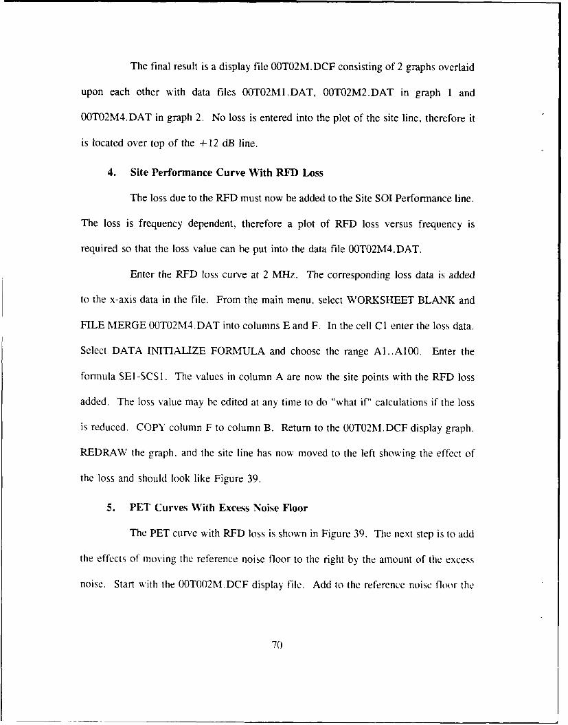
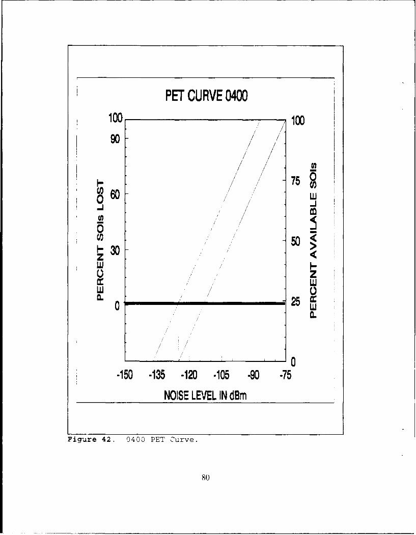
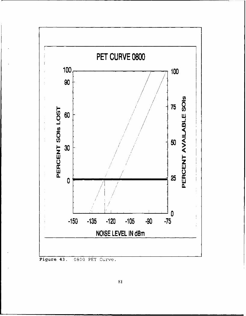
PET curves corresponding to the 4-hour intervals are shown in Figures 41-46. This
completes the preliminary work.
77

MAXIMUM SIGNAL STRENGTH PREDICTION
-70
..... .......................................... .....................Z \
'745
-9
Figure~ ~ ~ 4 . ................... P edi ted
-J
z
0 5 10 15 2
TIME OF DAY IN HOURS
Figure 40. Maximum Signal Strength Predicted.
78

PET CURVE 0000100 100
/ /
I... / 75U)60 wS/ /
50i30 /z
a: Li
, m, z
F E uv0.
-150 7135 -120 -105 -90 -75
NOISE LEVEL IN dBm
Figure 41. 0000 PET Curve.
79
PET CURVE 0400100 100
90~ / /
/ // /I-o / ,, 75iI
/ i' U
.o /
NU0 "
0.0
-150 -135 -120 -105 -9t0 -75
NOISE LEVEL IN dBm
Figusre 42. 0400 PET Curve.
80
PET CURVE 0800100 p100®//
//
/ / 75/7 //
/ /<
30 /W ,/ I-g
/ )/ Zo w0 0.
/ '
i/
0-150 -135 -120 -105 -90 -75
NOISE LEVEL IN dBm
Figure 43. 0800 PET Curve.
81

PET CURVE 1200100 100
7 0~60w
30 /cn in //
/ i //5
z <
LU
L 0
, /i , / , L ,
0I /
-150 -135 -120 -105 -90 -75
NOISE LEVEL IN dBm
Figure 44. 1200 PET Curve.
82

PET CURVE 1600100 100
/7, /
a //
// J
I 030 - <zw
w 0
o 250 0.
0-150 -135 -120 *105 -90 -75
NOISE LEVEL IN dBm
Figure 45. 1600 PET Curve.
83
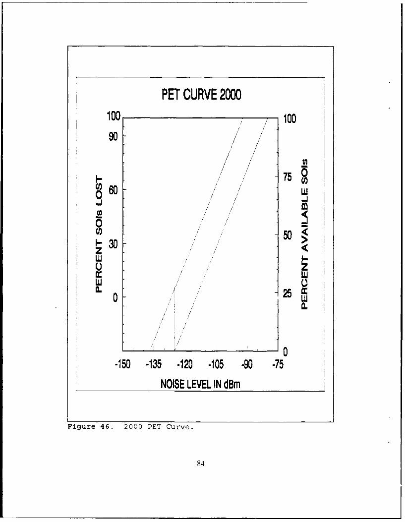
PET CURVE 2000100 / / 100
//75 00 LU
5030/
/ I LU
0 /LU
/ K 0-150 -135 -120 -105 -90 -75
NOISE LEVEL IN dBm
Figure 46. 2000 PET Curve.
84
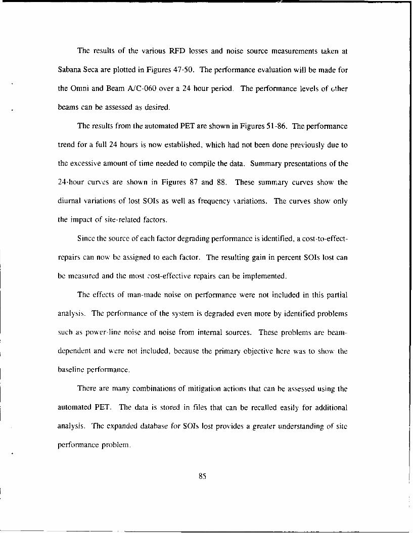
The results of the various RFD losses and noise source measurements taken at
Sabana Seca are plotted in Figures 47-50. The performance evaluation will be made for
the Omni and Beam AJC-060 over a 24 hour period. The performance levels of other
beams can be assessed as desired.
The results from the automated PET are shown in Figures 51-86. The performance
trend for a full 24 hours is now established, which had not been done previously due to
the excessive amount of time needed to compile the data. Summary presentations of the
24-hour curves are shown in Figures 87 and 88. These summary curves show the
diurnal variations of lost SOIs as well as frequency %ariations. The curves show only
the impact of site-related factors.
Since the source of each factor degrading performance is identified, a cost-to-effect-
repairs can now be assigned to each factor. The resulting gain in percent SOIs lost can
be measured and the most cost-effective repairs can be implemented.
The effects of man-made noise on performance were not included in this partial
analysis. The performance of the system is degraded even more by identified problems
such as power-line noise and noise from internal sources. These problems are beam-
dependent and were not included, because the primary objective here was to show the
baseline performance.
There are many combinations of mitigation actions that can be assessed using the
automated PET. The data is stored in files that can be recalled easily for additional
analysis. The expanded database for SOIs lost provides a greater understanding of site
performance problem.
85
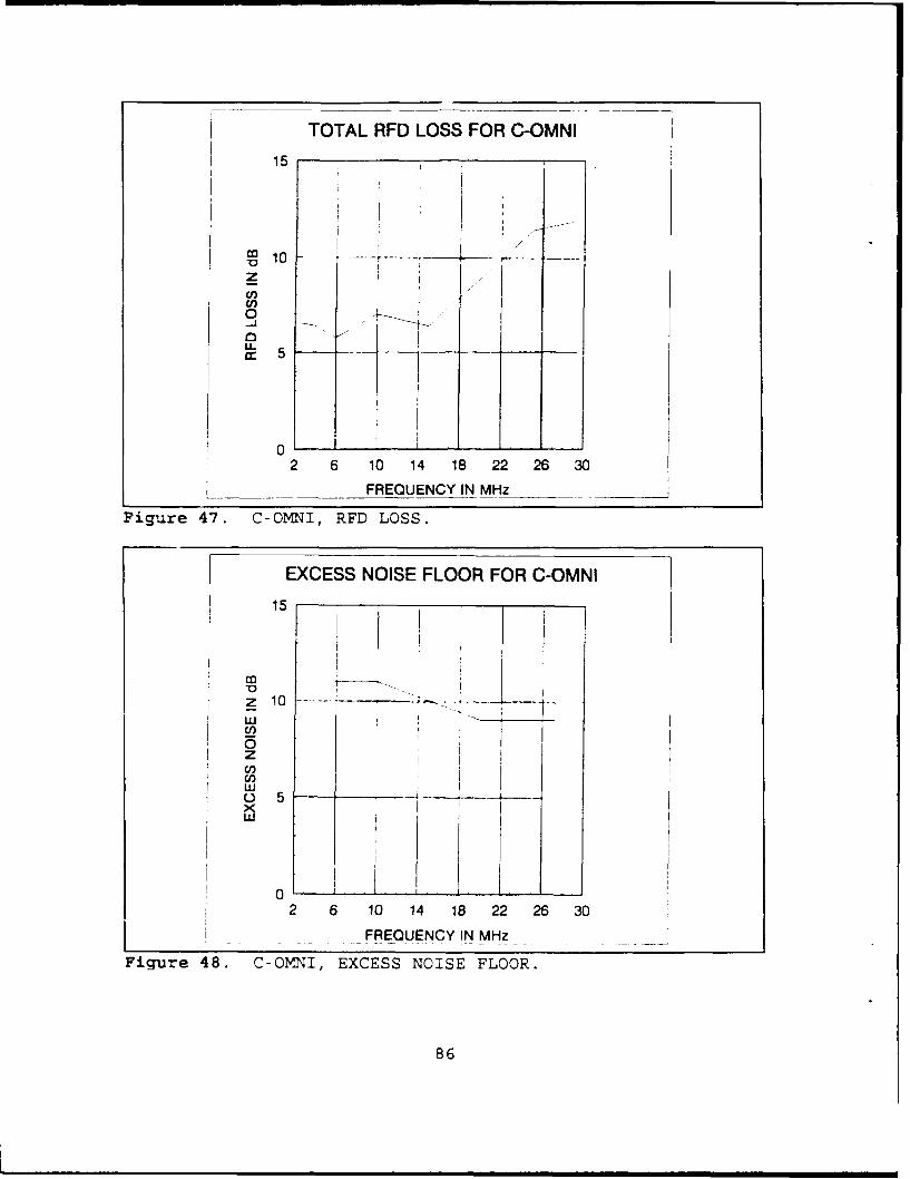
TOTAL RFD LOSS FOR C-OMNI
1 10
z
0
0
lr 5-- -
2 6 10 14 18 22 26 30
FREQUENCY IN MHz
Figu'.re 47. C-OMNI, RFD LOSS.
EXCESS NOISE FLOOR FOR C-OMNI
15
z 10
z
L) 5
0 I
2 6 10 14 18 22 26 30
FREQUENCY IN MHz
Figure 48. C-OMNI, EXCESS NOISE FLOOR.
86

TOTAL RFD LOSS FOR BEAM A/C-060
15 _ _ _ _
ZI C/0
cc
0
2 6 10 14 18 22 26 30
I FREQUENCY IN MHz
Figure 49. A\C-060, RFD LOSS.
EXCESS NOISE FLOOR FOR BEAM A/C-GGO
15 -_ _ _ _ _ _ _ _
Z 10 -_ _ _
U)
0 5--- -
x
0 1 L
2 6 10 14 18 22 26 30
FREQUENCY INMHz__J
Figure 50. A/C-O60, EXCESS NOISE FLOOR.
87

PERCENT SOIs LOST vs. FREQUENCY AT TIME 0000DUE TO RFD LOSS
100
90 iI , _C-OMNI
80I- _ _ _ _
O 70 -t
U 40
30
0
20
2 6 10 14 18 22 26 30
FREQUENCY IN MHz
Figure 51. C-OMNI, RFD, 0000.
PERCENT SOIs LOST vs. FREQUENCY AT TIME 0400DUE TO RFD LOSS
= , C-OMNI10
cn 70
60 - -
0"'50
LU 40 6 10 - 4 -1 -22 6--C.)wu 30(L
20
1
2 6 10 14 18 22 26 30FREQUENCY IN MHz
Figure 52. C-OMNI, RFD, 0400.
88

PERCENT SOIs LOST vs. FREQUENCY AT TIME 0800
DUE TO RFD LOSS10090 ... .
C-OMNI8070060 I
0
') 50 -I-Iz,, 40 --L)w 30
20
10
02 6 10 14 18 22 26 30
FREQUENCY IN MHz
Figure 53. C-OMNI, RFD, 0800.
PERCENT SOIs LOST vs. FREQUENCY AT TIME 1200DUE TO RFD LOSS
100
90 •_ _C-OMNI80
70
600co 50
w 40
w 30C2
20
10
02 6 10 14 18 22 26 30
FREQUENCY IN MHz ...
Figure 54. C-OMNI, RFD, 1200.
89

PERCENT SOIs LOST vs. FREQUENCY AT TIME 1600
DUE TO RFD LOSS100
80 C-OMNI80 q'
"'70oJ0
50I-'ZW 40.i0
w 30
20
10
02 6 10 14 18 22 26 30
FREQUENCY IN MHz
Figure 55. C-OMNI, RFD, 1600.
PERCENT SOIs LOST vs. FREQUENCY AT TIME 2000
DUE TO RFD LOSS100 I
80[ I_ _ -C-OMNI
I.-.Ci) 70
w 40
_J
C-'
20-
10
02 6 10 14 18 22 26 30
__ FREQUENCY IN MHz
Figure 56. C-OMNI, RFD, 2000.
90

PERCENT SOIs LOST vs. FREQUENCY AT TIME 0000DUE TO EXCESS NOISE FLOOR100 i
i if C-OMNI80 ----
70 __ __ __ ____
0
w30
020
10
2 6 10 14 18 22 26 30
FREQUENCY IN MHz
Figure 57. C-OMvflI, EXCESS NF, 0000.
PERCENT SOls LOST vs. FREQUENCY AT TIME 0400DUE TO EXCESS NOISE FLOOR
100
90+ C-OMNI
80
] F
"70 I060
0
50WU 40 - _ _ _ _
L,
wu 30
20
10
2 6 10 14 18 22 26 30
FREQUENCY IN MHz
Figure 58. C-OMNI, EXCESS NF, 0400.
91

PERCENT SOIs LOST vs. FREQUENCY AT TIME 0800DUE TO EXCESS NOISE FLOOR
10090 '90 !C-OMNI
80
"' 70
6050 .
I-zw 40
w 30
20
10
2 6 10 14 18 22 26 30
____ ___ FREQUENCY IN MHz
Figure 59. C-OMNI, EXCESS NF, 0800.
PERCENT SOls LOST vs. FREQUENCY AT TIME 1200DUE TO EXCESS NOISE FLOOR100~~_
C-OMNI80 - _ _
C"70--- I060
0
C)w 4 ~r
w 300.
20
1!
2 6 10 14 18 22 26 30
FREQUENCY IN MHz
Figure 60. C-OMNI, EXCESS NF, 1200.
92
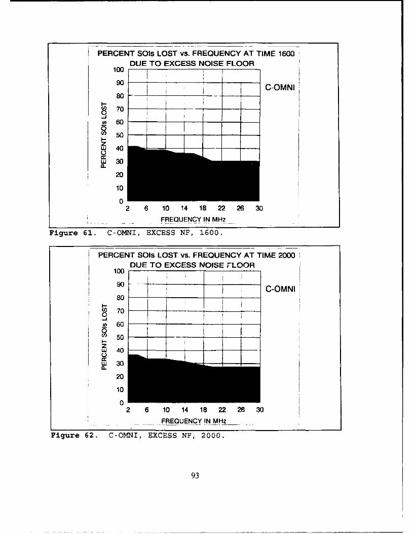
PERCENT SOIs LOST vs. FREQUENCY AT TIME 1600DUE TO EXCESS NOISE FLOOR
1001
8 C-OMNI80
7 0Qo
0) 60 ----
"' 50ZW 40
w 30
20
10
0
2 6 10 14 18 22 26 30FREQUENCY IN MHz
Figure 61. C-OMNI, EXCESS NF, 1600.
PERCENT SOIs LOST vs. FREQUENCY AT TIME 2000DUE TO EXCESS NOISE FLOOR
100
90~j_ _
C-OMNI80
C'l 70
in60
o 50
zw 40
cc30
20
10
o
2 6 10 14 18 22 26 30
FREQUENCY IN MHz
Figure 62. C-OMNI, EXCESS NF, 2000.
93

PERCENT SOIs LOST vs. FREQUENCY AT TIME 0000DUE TO E' ESS NOISE FLOOR AND RFD LOSS100
9 IC-OMNI8070
0-j
600
Z"u 40L-
cc
20
1020
2 6 10 14 18 22 26 30
FREQUENCY IN MHz
Figure 63. C-OMNI, RFD AND EXCESS NF, 0000.
PERCENT SOls LOST vs. FREQUENCY AT TIME 0400DUE TO EXCESS NOISE FLOOR AND RFD LOSS100
90 C-OMNI
8070
0
60
400
W 400
20
10
02 6 10 14 18 22 26 30
FREQUENCY IN MHz
Figure 64. C-ONI, RFD AND EXCESS NF, 0400.
94
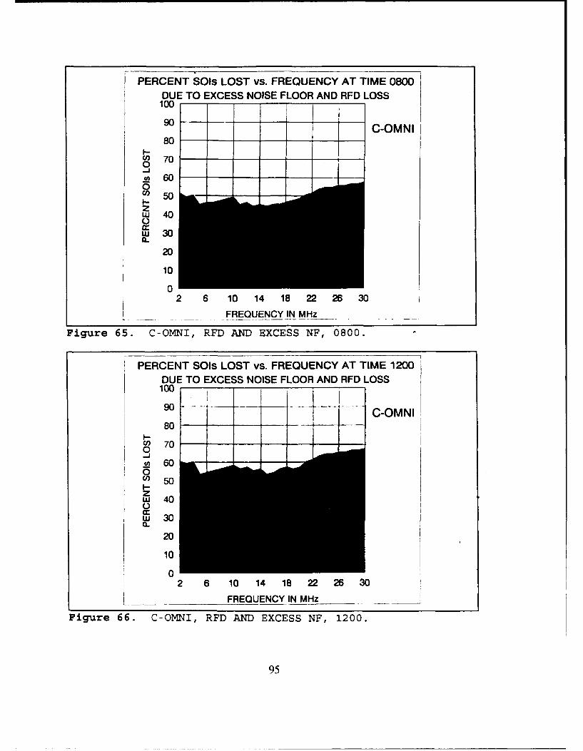
PERCENT SOIs LOST vs. FREQUENCY AT TIME 0800DUE TO EXCESS NOISE FLOOR AND RFD LOSS
100
-- C-OMNI80
U) 700_j2 6O0Cl 5 0I.-zw 400c.w 300.
20
10
02 6 10 14 18 22 26 30
FREQUENCY IN MHz .
Figure 65. C-OMNI, RFD AND EXCESS NF, 0800.
PERCENT SOIs LOST vs. FREQUENCY AT TIME 1200DUE TO EXCESS NOISE FLOOR AND RFD LOSS100
I-90 C-OMNI
80
U70--_1-0
M600c 50I-zW 40
w, 30a-
20
10
2 6 10 14 18 22 26 30
FREQUENCY IN MHz
Figure 66. C-OMNI, RFD AND EXCESS NF, 1200.
95

PERCENT SOIs LOST vs. FREQUENCY AT TIME 1600DUE TO EXCESS NOISE FLOOR AND RFD LOSS100
90C-OMNI80 ,
I-Ci 700-J 60
"'50zw 400w 30IL
20
10
02 6 10 14 18 22 26 30
FREQUENCY IN MHz
Figure 67. C-OMNI, RFD AND EXCESS NF, 1600.
PERCENT SOIs LOST vs. FREQUENCY AT TIME 2000DUE TO EXCESS NOISE FLOOR AND RFD LOSS100
90 C-OMNI
I- I.O60
0
U" 50I-
w 40
w 30(.
20
10
02 6 10 14 18 22 26 30
FREQUENCY IN MHz
Figure 68. C-OMNI, RFD AND EXCESS NF, 2000.
96

PERCENT SOIs LOST vs. FREQUENCY AT TIME 0000DUE TO RFD LOSS
100190) __BEAM
80 A/C-060
I-'"' 700W 600n 50
zw, 40
0L)w 30
10
20
10
0
2 6 10 14 18 22 26 30
FREQUENCY IN MHz
Figure 69. A/C-060, RFD, 0000.
PERCENT SOIs LOST vs. FREQUENCY AT TIME 0400DUE TO RFD LOSS
100
90 - • BEAM__ i A/C-060
80 . .. . .. ..
U) 700-.,, 60 --
z0Lu 40 . . .
w 30
20
10
0
2 6 10 14 18 22 26 30
FREQUENCY IN MHz
Figure 70. A/C-060, RFD, 0400.
97

PERCENT SOIs LOST vs. FREQUENCY AT TIME 0800DUE TO RFD LOSS
100
9 , BEAM80 __ A/C-060
C" 70 t _0
S60
z' 50
w 40
20
10
02 6 10 14 18 22 26 30
----------- FREQUENCY IN MHz
Figure 71. A/C-060, RFD, 0800.
PERCENT SOIs LOST vs. FREQUENCY AT TIME 1200DUE TO RFD LOSS100 [.L
10 ... ,- BEAM
80 - V A/C-06080.. . . .
C 700
m 50I--zw 0
Lu 3020
10
02 6 10 14 18 22 26 30
FREQUENCY IN MHz
Figure 72. A/C-060, RFD, 1200.
98

PERCENT SOIs LOST vs. FREQUENCY AT TIME 1600DUE TO RFD LOSS00 __ BEAM
801 A/C-060
U~700°-J_60
0I-zw 400I~rw 30
10
0
2 6 10 14 18 22 26 30
FREQUENCY IN MHz
Figure 73. A/C-060, RFD, 1600.
PERCENT SOIs LOST vs. FREQUENCY AT TIME 2000DUE TO RFD LOSS
100 BEA9o _ BEAM
90 _ A/C-0608o
cn 70 ' '0 ,
U/ 60 -
0co 50zLu 40I-w 300
20
10
02 6 10 14 18 22 26 30
FREQUENCY IN MHz
Figure 74. A/C-060, RFD, 2000.
99

PERCENT SOIs LOST vs. FREQUENCY AT TIME 000DUE TO EXCESS NOISE FLOOR
100
90 BEAM__ __ ______A/C-06
80 --C" 70
0n 60
S50__ i50
w 40 -- _
L 3020
10-
02 6 10 14 18 22 26 30
FREQUENCY IN MHz
Figure 75. A/C-060, EXCESS NF, 0000.
PERCENT SOIs LOST vs. FREQUENCY AT TIME 0400DUE TO EXCESS NOISE FLOOR
100
90 BEAMI A/C-060
80
U) 70-0
() 60 600
5030
(L
20
1
2 6 10 14 18 22 26 30
_ _ FREQUENCY IN MHz
Figure 76. A/C-060, EXCESS NF, 0400.
100

PERCENT SOIs LOST vs. FREQUENCY AT TIME 0800DUE TO EXCESS NOISE FLOOR
100
!90 BEAMIo ' A/C-060
80 -
70 --00
"'50I-zW 40
w 300.
20
10
02 6 10 14 18 22 26 30
FREQUENCY IN MHz
Figure 77. A/C-060, EXCESS NF, 0800.
PERCENT SOIs LOST vs. FREQUENCY AT TIME 1200iDUE TO EXCESS NOISE FLOOR
10090 BEAM
8 I A/C-06080
Wn 70
50
z,,, 40C-)Iw 30
20
10
02 6 10 14 18 22 26 30
FREQUENCY IN MHz
Figure 78. A/C-060, EXCESS NF, 1200.
101

PERCENT SOIs LOST vs. FREQUENCY AT TIME 1600DUE TO EXCESS NOISE FLOOR
90 _BEAMI 'A/C-060
80 - 4 -
U 70 _o I-J
60
U, 50I--zw 40
0uw 30
20
10
0
2 6 10 14 18 22 26 30
FREQUENCY IN MHz
Figure 79. A/C-060, EXCESS NF, 1600.
PERCENT SOIs LOST vs. FREQUENCY AT TIME 2000DUE TO EXCESS NOISE FLOOR100
90 _ BEAM80 A/C-060
80
700
60
cO50
ZLU 40
a.' 30 / .
20
10
o01 I
2 6 10 14 18 22 26 30FREQUENCY IN MHz
Figure 80. A/C-060, EXCESS NF, 2000.
102

PERCENT SOIs LOST vs. FREQUENCY AT TIME 0000DUE TO RFD LOSS AND EXCESS NOISE FLOOR
100
90 BEAM______ A/C-06080 -
S700-.J
02600I--zw 40
w 30a.
20
10
02 6 10 14 18 22 26 30
FREQUENCY IN MHz
Figure 81. A/C-060, RFD AND EXCESS NF, 0000.
PERCENT SOIs LOST vs. FREQUENCY AT TIME 0400DUE TO RFD LOSS AND EXCESS NOISE FLOOR
100 - .BA
90 BEAM----- 44...
8 0 - ~ tA/C-060-0 70
~0 60
a-
20
10!
50
2 6 10 14 18 22 26 30FREQUENCY IN MHz - _
Figure 82. A/C-060, RFD AND EXCESS NF, 0400.
103

PERCENT SOIs LOST vs. FREQUENCY AT TIME 0800DUE TO RFD LOSS AND EXCESS NOISE FLOOR
10090 1 I * BEAM90, i A/C-00
80----
-- 700-I
60Co50I-zW 400L.w 30CL
20
10
02 6 10 14 18 22 26 30
FREQUENCY IN MHz
Figure 83. A/C-060, RFD AND EXCESS NF, 0800.
PERCENT SOIs LOST vs. FREQUENCY AT TIME 1200DUE TO RFD LOSS AND EXCESS NOISE FLOOR
100
90 i BEAMA/C-060
80S70
0-j
cn 60
0C" 50
0w 30(0
20
10
02 6 10 14 18 22 26 30
FREQUENCY IN MHz
Figure 84. A/C-060, RFD AND EXCESS NF, 1200.
104

PERCENT SOls LOST vs. FREQUENCY AT TIME 1600DUE TO RFD LOSS AND EXCESS NOISE FLOOR
100 - _ _ _
90 ---- _--- BEAM80 A/C-0
U) 70 - - - -0u~60
C) 50
zw40
w 30C.
20
10
02 6 10 14 18 22 26 30
FREQUENCY IN MHz _
Figure 85. A/C-060, RFD AND EXCESS NF, 1600.
PERCENT SOls LQST vs. FREQUENCY AT TIME 2000DUE TO RFD LOSS AND EXCESSNOISE FLOOR
100- - --90-----------------------BEAM90 A/C-060
U, 700
.La 600I.- 5zW 40
w 30
20
10
02 6 10 14 18 22 26 30
FREQUENCY IN MHz
Figure 86. A/C-060, RFD AND EXCESS NF, 2000.
105

24 HOUR SOIs LOSTDUE TO RFD LOSS AND EXCESS NOISE FLOOF
100 -00oa-i 0400
90 "MN 1 c0800
80 --
w 40
F- J 1600 JU) 70 20 _0 _, -_
10 -~~50 TL.- 40
2 6 10w 14 18 22 26 30
FREQUENCY IN MHz
Figure 87. C-OMNI, RFD AND EXCESS NF, 24 HOURS.
24 HOUR SOIs LOSTDUE TO RFD LOSS AND EXCESS NOISE FLOOF
1 0 0 -" 0 4 0 0
90 ... 00800i 4/c-os 00 - 1200
60 107 0 z --2000
0
cn 50
w 40 ._
m 30 -
20
10 ! ' I
02 6 10 14 18 22 26 30
FREQUENCY IN MHz
Figure 88. A/C-060, RFD AND EXCESS NF, 24 HOURS.
106
VII. CONCLUSIONS AND RECOMMENDATIONS
A. CONCLUSIONS
Work accomplished under this thesis reached a number of conclusions. They are:
" It was verified that the amount of data required to complete a comprehensive studyof factors affecting the performance of a receiving site is too large to handle bymanual techniques. Only simple problems with restricted objectives can be handledby manual means.
" The usefulness of automated techniques for processing and formatting data neededfor a comprehensive analysis of site performance was demonstrated. Practicalexamples were produced from field data.
* The ability to define the impact of each factor that degrades site performance wasdemonstrated.
" It was shown that a cost can be associated with each factor that degrades siteperformance. This allows site managers to conduct accurate and meaningful cost-benefit analyses of the mitigation actions required to restore a site to higher levelsof performance.
" While the present automated PET process has been shown to be of high value,even further benefits can be obtained by writing custom computer software toreplace the standard data processing software used in this effort.
B. RECOMMENDATIONS
Based on the conclusions reached in this thesis, specific recommendations are:
" Dedicated computer software should be designed and written specifically toperform PET curve analyses.
* A number of problems exist in all CDAA sites, and in other receiving sites too,that need to be corrected. The PET process should be used to aid in planning allsite upgrades. modifications, improvements, and repairs that might impactperformance. Site managers should use the PET process to determine the amount
107

of performance improvement or degradation caused by each factor and relate thisto the cost of implementing each action.
" Additional studies of the amplitude probability distributions of certain classes ofSOIs are needed to support the full use of the PET.
* The methods used to predict and verify the maximum amplitudes of SOIs and othersignals need to be improved.
* A user's manual should be completed that describes all aspects of the PET processand provides simplified implementation procedures. This manual shouldaccompany the existing computer software and future dedicated software.
" A library of photos showing the spectral and temporal detail of noise from a largenumber of man-made sources is needed. The availability of such a library willsignificantly aid in the identification and location of the sources of noise.
108
APPENDIX A. NOISE MEASUREMENT SYSTEMS
SNEP teams have found it necessary to use special equipment to measure and
define the primary characteristics of man-made radio noise. This equipment provides the
amplitude versus frequency data needed for the PET process. It also provides sufficient
information to distinguish between external and internal sources of noise and to identify
the types of sources involved. The identification of the types of sources and their
individual impact on site performance is a key factor in developing effective mitigation
activities to correct the man-made noise problems.
A second source of noise data is also available. The Automatic Noise
Measurement System (ANMS) developed by the Naval Electronic Engineering Activity,
Pacific (NEEACT PAC) is available at many sites, and it provides routine measurements
of RFD noise levels. The objectives of the ANMS are to:
* Document changes to the ANMS measured site noise baseline over time or aftermitigation procedures are performed.
" Automatically measure strong signal levels at NAVSECGRU CDAA sites todetermine if they may cause intermodulation products in the sy stem.
* Develop a standard measurement technique which can be used to establish adatabase and compare measurements between NAVSECGRU sites.
The ANMS records noise power, and it provides limited noise analysis capabilities.
The current version of the ANMS does not provide the temporal and spectral information
required to identify sources of noise. Future versions of this system may provide
sufficient information for the complete PET analysis effort.[Ref. 1]
109
APPENDIX B. SNEP NOISE DEFINITION EQUIPMENT AND
CONFIGURATION
This entire appendix was drawn from Appendix A of the Doctoral Dissertation of LCDR
G. Lott [Ref. 3:pp. 172-178].
110
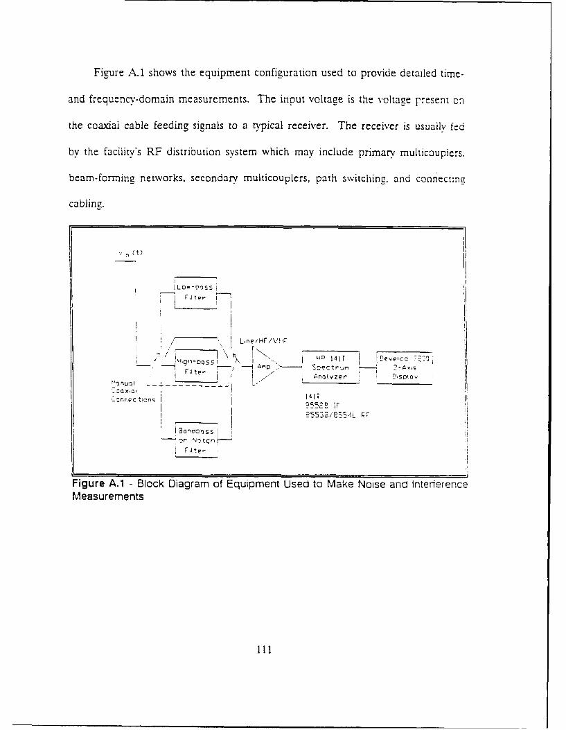
Figure A.1 shows the equipment configuration used to provide detailed t*ime-
and frequ encv-do main measurements. The input voitaae is the voltage present con
the coaxial cable feeding signals to a typical receiver. The receiver is usually fed
by the facility's RF distribution system which may include primary multicouplers.
beamn-for-nina networks, secondary multicouplers, path switching, and connectinpc
cabling.
L.4OIr~SS J141 T 7~ecc 7EO
.Z c 't~ns I~iPe552 IF
F4 tcn -
Figure A.1 - Block Diagram of Equipment Used to Make Noise and InterferenceMeasurements
While measurements are made with the spectrum analyzer connected directly
to the RF distribution system. filters and amplifiers can modify the input voltage.
The filters commonly used include a lowpass filter with a cutoff frequency of 1
MHz. a highpass filter with a 35 MHz cutoff frequency., and a bank of bandpass
filzrs designed to pass non-international broadcast bands from 2 to 30 MHz.
Strong sigmals may require the use of an external attenuator.
The amplifiers include a low frequency (10 Hz to 500 kHz) line amplifier, an
HF amplifier (such as the Olektron Model B-HL-11-HF, 500 kHz to 50 MHz),
and a VHF ampiifier (50 MHz to 500 MHz). The line and VHF amplifiers are
used primarily to make intermodulation products measurements above and below
the HF spectrum. The HF amplifier must have a large dynamic range, requiring
a third order intercept point of at least +52 dBm.
As shown in Figure A.1, the Hewlett-Packard (HP) Model 140/141 spectrum
analyzer acts as a scanning receiver. Along with the HP 141T Display Section.
typicai HF measurements require two plug-in modules, the HP 8552B Intermediate
Frequency Section and the HP 8553B RF Section. The operator can adjust the RF
attenuation, scan rate, scan width, IF gain, IF bandwidth, and other controls to give
the best presentation of the noise or signal under observation.
The Develco 7200 3-axds display provides a real time display of noise and
signals received with the spectrum analyzer. As shown in Figure A.2, the three
axes are usually frequency (horizontal axis), signal or noise power (vertical axis).
112

and time (depth or Z axis). The horizontal axis is also the time for each spectrum
analyzer sweep which allows measurement of repetition rate and duration of
wideband interference such as distribution power-line related noise.
~ RdesT Se'e'
/ ~~ ----- ------------------------------
- ~ ~ '.~ - .-.------ --------------------- ______________
L~test screen
F e quenc a £n a ~Hz, k H z, r Y -H z
Time or 1 Anal .. 'er Sweep (us, mns, K
Figure A.2 - Units of Measure Associated with Each Axis in Photo gracns Made
with the 3-Axis Display System
The HP141 spectrum analyzer provides two signals to the 3-axis display. video
and synch. The 3-axis display takes 512 equally spaced samples of the video signal
from each complete analyzer scan, and the sample resolution is eight bits. As
shown in Figure A.3, the Develco 7200 is a first-in, first-out (FIFO) display. The
latest scan appears as line one. Line one moves to line two with the newest scan
again appearing as line one. The 3-axis display can typically store up to 60
113
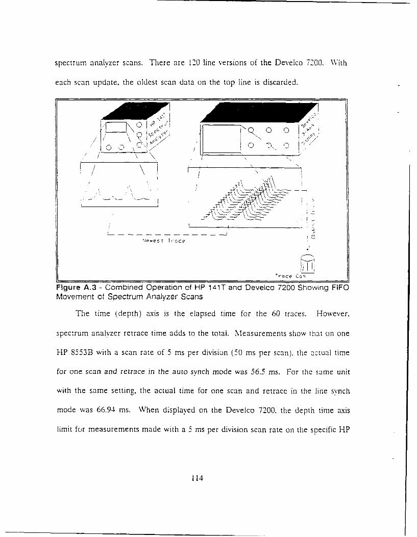
spectrum analyzer scans. There are 120 line versions of the Develco 7200. WVith
each scan update, the oldest scan data on the top line is discarded.
.0 0 7 ' _ 0__ 0___ _:__"/"/
"'A A
/ /
'Jewest I f'd
-. ~ W
T r,-, ce
Trace Can
Figure A.3 - Combined Operation of HP 141T and Deveico 7200 Showing FIFOMovement of Spectrum Analyzer Scans
The time (depth) axis is the elapsed time for the 60 traces. However,
spectrum analyzer retrace time adds to the total. Measurements show that on one
HP 8553B with a scan rate of 5 ms per division (50 ms per scan), the actual time
for one scan and retrace in the auto synch mode was 56.5 ms. For the same unit
with the same setting, the actual time for one scan and retrace in the line synch
mode was 66.94 ms. When displayed on the Develco 7200, the depth time axis
limit for measurements made with a 5 ms per division scan rate on the specific HP
114
8553B are 60 times the actual time for one scan plus retrace, or 3.4 s and 4.0 s
respectively.
There is no simple expression that one can use to determine the actual scan
time as a function of the instrument control scan rate. Prior to makina
measurements, the operator must measure the actual scan times for each scan rate
in both the auto and line synch modes. The actual scan times will be different for
each HP 8553B. and experience shows that the times will change each time a unit
undergoes calibration.
Measurements require accurate frequency. ampiitude. and time calibrations
for use as standards for manually scaling the photographs taken of the 3-axis
display's screen. Calibrations include the total scan time measurements and a 10
dB step amplitude calibration photograph. Calibrations are good only for the
specific instruments used. Operators should make daily checks to ensure that the
calibration photographs are accurate. Changing the oscilloscope camera may
require a new amplitude calibration photograph because image compression may
occur due to small differences in the camera lens.
Figure A.4 shows a sketched example for 25 spectrum analyzer scans as
displayed on the Develco 7200. The figure shows the temporal changes for six
signals in the 50 kHz part of the HF spectrum. Actual signal identification for
some modulation types is difficult using only the 3-axis display. To make signal
identification easier, a separate HF communications receiver augments the
measurement system.
115

E]rS CC~
Two StronCer / ,'Ce Panuw,ithFSJ-< S; os . ''"/oice, FAX, c. " e
// ,/ / / :K
17.
Time
L .- = --- rec 'gnrv H~Z) :2.60
Figure A.4 - Example of 3-Axis Display of HF Signals
The 3-axis display controls allow for:
+ freezing the data in memory for photographing or detailed viewing
+ changing amplitude compression
+ changing the elevation and azimuth of the depth axis
# adjusting the background level.
To make photographs for amplitude measurements, the display elevation and
azimuth are set to zero. This results in viewing all 60 traces as if they were
superimposed into one trace. Using a card made from the 10 dB calibration step
photograph, knowing the equipment settings, and using the trace baseline as a
reference, one can manually scale the amplitude photographs.
116

Controls also allow for the selection and display of subsets of the 60 spectrum
analyzer scans stored in 3-axis display memory. Experience using the 3-axis display
while viewing various types of signals and noises results in the operator being able
to adjust the 3-axis display controls to optimize the presentation. A typical
measurement requires two photographs, one for amplitude measurement and one
with the time (depth) axis elevated to show temporal variations.
117

APPENDIX C. PROPHET SIGNAL STRENGTH COMPUTATION
PROPHET provides a convenient way to predict the value of the maximum signal
strength of received signals. The following parameter list specifies the input information
for a signal strength calculation. A sample set-up procedure is also provided.
* AT- Atmospheric Noise- No
* BW- Bandwidth- 3.00 kHz
s DA- Set Date- 12/1/91
* FL- 10.7 cm Flux- 145.0
0 FR- Frequency Input- 2-30 MIHz
0 LA- Launch Angle- 1.0 Deg. Min., 87.0 Deg. Max.
0 NM- Numeric Units- Kilometers
* NP- Propagation Modes- 6
* RN- Receiver Name- Sabana Seca
* TN- Transmitter Name- TEMPXMTR
0 WI- Wind Velocity- 1 Knot
* XF- X-Ray Flux- 1.OE-03
The previous list of set-up information can be listed by typing LI while in the
PROPHET program. Assign the receiver as PTRICO and designate a new transmitter
118

as TEMPXMTR with the desired antenna characteristics. The following is the set-up
definition of TEMPXMTR:
0 TEMPXMTRLat. 29.5 W., Lon. 51.3 N., OMNI Ant., 1000 W.
The resulting Signal Strength calculation for the times listed is in dBuV.
To convert the signal strength in dB above a microvolt into dBm use the conversion
SS dBuv - 107 = SS dBm (2)
The value that is obtained is the maximum signal strength expected to be used in the PET
curves to set the amplitude distribution of SOIs. Figures 89 and 90 are the desired
outputs from PROPHET.
119

UNCLASSIFIED ***DATE: 12/ 1/91 ATMOSPHERIC NOISE: NO10.7 CM FLUX: 145.4 X-RAY FLUX: .0010 MAN-MADE NOISE: QMTEMPXMTR LAT: 29.5 LON: 51.3 ANT: 101 @ *OMNI* PWR: 1000.00PTRICO LAT: 18.0 .ON: 66.5 ANT: 0 @ *OMNI* RANGE: 2003 KM
SIGNAL STRENGTH (DB ABOVE 1 MICROVOLT)
FREQUENCYTIME 2 8 16 24 32 40 LF MF00 29 33 32 31 29 26 11-15 2 1301 29 32 32 30 28 24 0 2 1202 29 32 32 30 27 24 -2 2 1203 29 32 31 29 26 15-14 2 1104 29 32 31 28 25 6 2 1105 29 32 31 29 25 11-18 2 1106 29 32 30 28 24 -2 2 1007 29 32 30 27 20 -9 2 1008 29 31 29 25 -1 2 809 29 31 28 24 -2 2 810 31 33 33 32 31 30 28 26 24 3 2 1911 -2 18 24 27 27 27 27 26 25 23 18-17 3 24
SIGNAL STRENGTH (DB ABOVE 1 MICROVOLT)
FREQUENCYTIME 2 8 16 24 32 40 LF MF
12 -3 13 20 23 24 25 25 24 23 21 11-11 4 26
13 -19 4 14 19 22 24 24 24 23 22 12 10-16 5 28
14 -3 10 16 20 22 23 23 23 22 13 11 -5 6 29
15 -6 8 15 19 22 23 23 23 22 13 12 0 6 2916 -7 7 14 18 22 23 23 23 22 13 12 0 6 29
17 -5 8 15 19 22 23 23 23 22 13 12 -6 6 29
18 0 12 17 21 23 24 24 23 22 13 9-16 5 28
19 -22 8 16 21 23 25 25 24 23 22 13 -7 -7
20 6 18 23 25 26 27 26 25 24 22 -4 4 25
21 :1 = 28 30 30 30 29 29 27 25 23 -2 z22 21 23 33 32 31 30 28 26 19 -8 -
23 29 33 33 31 30 28 25 10-18 2 15FS>
Figure 89. Maximum Signal Strength Prediction.
120

laga4 C-I
z1 -411
zz z A~
1.3-z
4M w
,ca " ca C
04 ̂3 ccI
I-CD
w~w01 I:
Figue 90 Grp fmxmmSgalSrnt rdcin
ax.121

APPENDIX D. HF SIGNAL AMPLITUDE STATISTICS
This entire appendix was drawn from Chapter III of the Doctoral Dissertation by LCDR
G. Lott [Ref. 3:pp. 28-45].
122
III. HF SIGNAL AMPLITUDE STATISTICS
This dissertation will use the random variable vin as the rcot-mean-
square (RMS) amplitude of the total, intercepted HF voltage applied to a receiver.
In a wideband receiver searching the HF spectrum for new signals, v,, represents
a voltage comprised of all broadcast signals. non-broadcast signals. and noise.
Distortion in non-linear RF system components, losses in cables and connectors.
ani induced noise add an undesired component to vi.
A wideband receiver and the first stages of many narrowband receivers must
be capable of processing the maximum peak value of vin. A narrowband receiver
with pre-selection will reject signals and noise outside the pre-selector bandwidth.
A much lower value of the input voltage will reach the front-end components of
a narrowband receiver with pre-selector filtering.
The RNIS voltage produced only by signals of military interest is considerabiv
different than v,,. It will have a smaller dynamic range than v. Analog-to-digital
(AID) converters designed to optimally quantize signals of military interest should
not waste limited quantization dynamic range on the high amplitude broadcast band
signals. Instead, the AID design should optimize the ability to receive and process
the adversary's most clandestine transmitter.
123
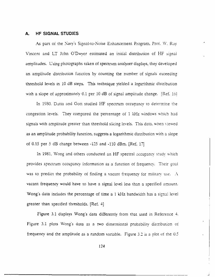
A. HF SIGNAL STUDIES
,As part of the Navv's Signal-to-Noise Enhancement Program. Prof. W. Ray
Vincent and LT John O'Dwvyer estimated an initial distribution of HF signal
amplitudes. Using photographs taken of spectrum analyzer displays, they developed
an amplitude distribution function by counting the number of signals exceeding
threshold levels in 10 dB steps. This technique yielded a logarithmic distribution
%kith a slope of approximately 0.1 per 10 dB of signal amplitude change. [Ref. 16]
In 1980. Dutta and Gott studied HF spectrum occupancy to determine the
congestion levels. They compared the percentage of 1 kHz windows which had
signals with amplitude greater than threshold slicing levels. This data, when viewed
as an amplitude probability function, suggests a logarithmic distribution with a slope
of 0.15 per 5 dB change between -125 and -110 dBm. [Ref. 17]
In 1981, Wong and others conducted an HF spectral occupancy study which
provides spectrum occupancy information as a function of frequency. Their goal
was to predict the probability of finding a vacant frequency for miitar, use. A
vacant frequency would have to have a signal level less than a specified amount.
Wong's data includes the percentage of time a 1 kHz bandwidth has a signal level
greater than specified thresholds. [Ref. 4]
Figure 3.1 displays Wong's data differently from that used in Reference 4.
Figure 3.1 plots Wong's data as a two dimensional probability distribution of
frequency and the amplitude as a random variable. Figure 3.2 is a plot of the 0.5
124
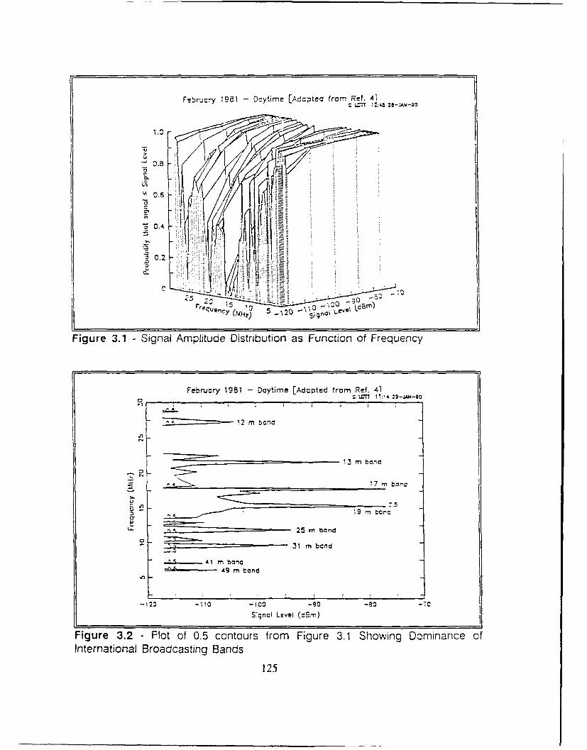
Februcry 1981 -Ocytime [Adopted from Ref. 41QLI.T !:4 26-;kA4-20
1.41
0.4
o0.2
2 eu~ 52 9 ~~
Figure 3.1 Signal Amplitude Distribution as Function of Frequency
February 1981 -Daytime [Adopted from Ref. 41torT ir1 ~.AJO
____________ 12 mn band
13 mn bond
17 bo .
- 19 M torc
25 rn bond
_________________ 31 mn bcnd
~- 49 mn bond
-120 -1 10 -l00 -90 -00 -70
S:9ncl Level (darn)
Figure 3.2 - Plot of 0.5 contours from Figure 3.1 Showing Dominance ofInternational Broadcasting Bands
125

probability contours from the surface in Figure 3.1. It clearly shows the dominance
of sinnls in the international broadcasting bands. Nearly all signals exceednz tnle
0.5 contours are within ITU allocated broadcasting bands.
P.A. Bradley, analyzing Wong's data, cencluded "...that occupancy (or
congestion) vanes with the threshold level (expressed in dBm) approximately in
accordance with a log-normal law." Of particular note is the limitation in Wong's
measurement system that allowed it to revisit each 1 kHz frequency window only
once every 3 to 5 days for one second duration. [Ref. 4]
Wilkinson performed a spectrai occupancy study in which he separa:td data
by frequency and receiver bandwidth. Figure 3.3 displays Wilkinson's data using the
same type of presentation as that in Figure 3.1. He found that cumulative signal
level distributions remain log-normally distributed for receiver bandwidths from 0.1
to 100 kHz. [Ref. 18]
Gibson and others conducted one of the few spectral occupancy studies using
a large aperture antenna, namely a circularly disposed antenna array (CDAA) or
Wullenweber antenna. After analysis, they concluded that the cumulative amplitude
distributions "...are found generally to follow a log-normal law." [Ref. 19]
Moulsley used an active-antenna-based observation system to make his spectral
observations. As shown in Figure 3.4, he found signals in the international
broadcasting band to have power levels more than 20 dB higher than signals in the
126

2 kHz Scrct h [Adoztea from Ref. 181L ~C L17r ":-27 '"-kN
'~0.21
c
;0.,00.2
Figure 3.3 - Signal Amplitude Distribution as Function of Frequency
3 kHz Eanowidth [Adopted from Ref. 201
o' 0
0
C- a-6 M? .20 U
I-~
-12 -1C • F -5 -4 -
0, Ox
Fiur 3. -. Bradasin vs.5 No-raca' Sga mliueDstiuin
2127
- 20 - C0 - 50 -40 -2 0S ILevel (d~m)
Figure 3.4 - Broadcasting vs. Non-Broadcasl ng Signal Amplitude Distributions
127

fixed, mobile, and maritime service bands. MNoulslev's data shows an amplitude
cumulative probability distribution which follows a log-normal law. [Ref. '0]
During the summer of 1987, Gibson performed a new spectral survey using
a technique different from his 19S1 observations. This study found little difference
in spectrum occupancy from weekdays to weekends. Gibson modeled the noise
floor as incident-external noise limited and distributed according to a Rayleigh law.
Even with this projection, he found that the overall amplitude cumulative
probability distribution followed a log-normal law. He eventually used a log-normal
model for the noise floor. This survey considered specifically signals in non-
broadcast portions of the HF band. This signal distribution should be similar to
that expected from signals of military interest discussed earlier. Figure 3.5 displays
the results. [Ref. 21]
Laycock and others made additional spectrum occupancy measurements in
central England using a format similar to Wong's 1981 survey. From this they
developed a model of channel occupancy, which is binomiallv distributed. While
similar, channel occupancy is different from amplitude cumulative probability.
Figure 3.6 shows the results of this study in a format similar to that used to show
data from Wong's study. [Ref. 22]
Another study in 1987 by Perry and Abraham suggests that the channel
occupancy statistics change when using bandwidths less than 150 Hz. The HF
channel-occupancy to power-level relationship found in this study is log-log
128
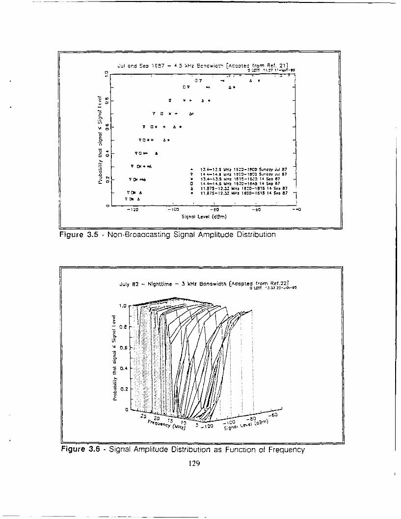
Jul and Seo 1S 87 -4,5 kHz Ecrlwidth [A~cnted from Ref. 2110 - L0C1T T11D7 11-40-900
a x M+ 60
Cj V 13x +. A.
is 134-13.9 V.HZ 1S.3-18ACO SUMOVY Jul 87V 14 4-14.g LAH2 I 5CO- I 5C SU'le-Y 'QI 87
7 DC40 x 13.4-13.9 M4Hz 1615-16.!0 14 Sep 870 0 14.4-14.0 M4Hz 1620-16A3 14 San 87
A 91.75-12.13 M~iz 1VOC-1515 14 Sep 37A0 11.275 - ,2.5.3 MHz : 6C0-1615 14 S.; 8
-120 -Ica -80 -'0
Signal Level (d~rm)
Figure 3.5 -Non- Broadcasting Signal Amplitude Distribution
July 132 -Nighttime -3 kcHz Bandwidth [Adopted from Ref.221c u:TT i_:1
1.0
-
C,
25 -63
0.2 /1 -;o
Figure 3.6 - Signal Amplitude Distribution as Function of Frequency
129

distributed. However, the model ignores curvature at the lower power levels due
to external noise. To simplify the data required for their work. Perr, and Abraham
normalized all measurements to the largest interferer, or signal. present. This
relationship is nearly log-normal after adding curvature on the extremes. [Ref. 23]
The most exhaustive HF signal level study published is that by Hagn and
others using measurements from Europe and the U.S. taken during the Fall 1987.
Most earlier studies used time averaged amplitude values, or they had long revisit
times to each 1 to 3 kHz window. Hagn's survey used instrumentation that allowed
rapid revisit. "Each of the 9333 3-kHz channels in the band from 2 :o 30 MHz was
sampled 150 times/hour...." [Ref. 24]
Figure 3.7 displays some of Hagn's data, and it reveals three significant results.
First. Hagn's data follow a log-normal distribution. The slope, which indicates
variance, is similar to the other tests conducted in Europe. However, the slope is
steeper for the U.S. tests. The smaller variance indicates a smaller dynamic range
requirement for receivers at sites in the continental U.S. environment.
Second, the mean signal level in the fixed and maritime service bands are
about 20 to 30 dB below the mean of signals in the international broadcast bands.
This agrees well with Moulslev's data as shown in Figure 3.4.
Third, there is a 10 to 30 dB difference in mean between signal levels in
Europe and signals in the U.S.. One would expect this since most European area
130

2 k.Hz Ecaw~ath [A-ed '!rri Ref. 241
-6
70 0+ +
0
a A
n Fied Sevice Arnovo
F-4,50 Sar.4ce Socianmetma Mcnitirm Ser"vic Seckennein.1
M x -.- A A Srcadclt Service Secxvntelm
I 2 CO -3 0 -C0 -,A0 -20]
S=iqncl ILevei (d ,rn)
Figure 3.7 - European and CONUS Signal Amplitude Distributions
transmissions are a single ionospheric hop from many powerful transmitters, and
many of the U.S. received signals are multi-hop from such sites.
Figure 3.8 shows the composite distributions from the various studies of non-
broadcast signals. To reduce the number of data points displayed in Figure 3.8,
the data representing Wong's and Laycock's studies (from References 4 and 22) are
displayed as the arithmetic mean over all frequency bins calculated with each non-
broadcast frequency bin as an independent observation.
B. THE LOG-NORMAL DISTRIBUTION
One common thread for all the studies is that they are normaliy distributed
when plotted as a function of received signal power in dBm. This leads one to
131

G LT !a M V
7500 7 4 - 9 +. + ~
:N 40 44 1 x7
' : 444 43 0 7V
1 4+o 0 7V~7 44. a Ref. 4. Rof. 15 1+4 Raf. 19
$ Ref. 21A Raf. 22
~40 V -& ~0 Rd. 24
Sgricl Level (c9.r)
Figure 3.8 -Composite of Non- Broadcasting Signal Amplitude Distributions
the log-normal distribution for the RMNS voltage v i at the input to a wideband
receiver.
The log-normal distribution is a positive. skewed distribution when plotted
aigainst a linear ordinate. Where the domain of the random variable for a normal
distribution is all of the real numbers. the domain of the random variable for a loc-
normal distribution is all non-negative real numbers.
Economic trends, biological growth. and particle size commonly describe
statistics that appear to be log-normally distributed (Ref. 251. Reference 25 is thle
universally accepted reference on the subject. Many other references which
132

mention the log-normal distribution simply summarize the Aitchison and Brown
[Ref. 25] work.
The random variable vin represents the composite RMS voltage amplitude as
described before, and w in is the composite power received. With a 50 2 load at
the receiver, the relationship between win and vi, is given by the expression:
Win = 20 1gio[ .(50)103) 1 (3.1)
where win is in dBm. vi, is in RMS volts such that v,,>0, and log,0 is the
logarithm to base 10.
When plotted as win' a normal distribution shape is the first indication that
v i, may be log-normally distributed. The next step in fully describing the
distribution is to calculate the mean and variance of the distribution of win, denoted
as /dB, and c2dm respectively. Assuming normalitv in the dBm domain, the
probability density of w~i is given by:
2(Uin'Udgmj
i 202m
PWi n(Win) 2 1 e .dm (3.2)ii, N27ra7dem
To simplify calculations, one can write wi, as a natural logarithm rather than
the decibel expression. Converting Equation 3.1 yields:
Win = 8.69 ln(Vin) + 13.01 (3.3)
133

Writing the density function of the RMS voltage amplitude vi, requires a
change of variable. Using the transformation,
andnVn = pi(Wi dwi (3.4)
and,
dwin 8.69 (35)va- i. n vin 35
the probability density function for the RMS voltage amplitude vir is given as:inin.'8.69 tntv in, -13 .01-u q i.
2
Pv ''Vi" 8.69 e 2 O'dBm (3.6)V i nN2TO!Bm
Makcing the substitutions
(dB,- 1 3 ..01'tnM - 8.69 (3.7)
and
0 dBm (3.8)In - 8 .69 '
the resulting distribution for the RMS voltage amplitude is:
(ln(vin) ;"tn J2
2_ 1 2 otn
PVin(Vin) n 2 e (3.9)V n 2 7rat n
which is the basic form of the log-normal distribution as used in Reference 25. The
received RMS voltage amplitude Will be positive since RMS implies the positive
square root. Thus vi >0 as required by the domain of the function.
134

Using the same notation as in Reference 25. one can write a mean and
variance for the distribution of v which gives the mean, a. in rms volts as:
1 2
and the variance. 13, as:
The mean and variance, calculated using Equations 3.10 and 3.11, provide an
intultive feel for the averace RMIS voltage levels of the receiver input. Othevise,
most calculations remain in the logarithmic domain where the fcrm of the
distribution is well understood. The density function in Equation 3.9 involves both
v in and In(vi, ) . There is no simple closed-form expression for the density function
in terms only of vin. [Ref. 251
An important result to be applied for the log-normal distribution is in the
application of the central limit theorem. Simply stated, in non-logarithmically
related distributions, the sum of independent random variables having the same
probability distribution will asymptotically become a gaussian distribution.
A similar statement for the log-normal distribution is possible for the product
of the random variables. In positive log-normal independent variates having the
same means and variances, the product of the variates is asymptotically log-normally
distributed. [Ref. 25]
135

This can be an important tool in estimating the products of the random
variable v: caused by non-linearities in the RF system. These products are the
resulting intermodulation products which add as noise to the desired signal.
C. ESTIMATING MEAN AND VARIANCE
The problem here is to match an experimentally determined cumulative
probability distribution function or probability density function to a theoretical
function. The two dependent variables to be applied in the match are the mean
and variance. To simplify calculations. the matching for HF signal studies is done
in dBm. The goal is to match a normal distribution to the experimental
observations. The following summarizes the mean and variance estimation methods.
1. Quartile Estimation
A simple method exists to fit a normal probability density function to
an experimentally derived histogram based on quartiles. Let N be the total number
of observations. The observations are ordered in histogram form. Starting with the
ordinate ha,,ing the smallest value, the first quartile is the ordinate value
corresponding to N/4 observations. etc. Stated differently, the first quartile is the
ordinate value for which one-fourth of the observations have a value less than or
equal that ordinate. The second, third, and fourth quartiles have similar definitions.
The second quartile is the observational median.
Croxton used a quartile rule to provide an estimate of the mean and
standard deviation of fitting a normal density based on these quartiles. [Ref. 261
136
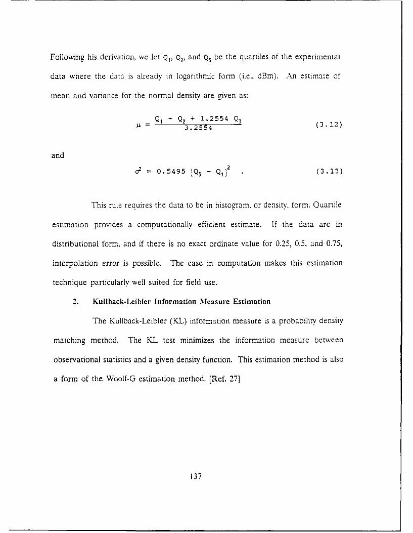
Following his derivation, we let Q1, Q2, and Q3 be the quartiles of the experimental
data where the data is already in logarithmic form (i.e., dBm). An estimate of
mean and variance for the normal density are Oven as:
Q1 +" Q2 + 1.2554 Q3 (.23.2554 (3.12)
and
2= 0.5495 (Q3 - Q .' (3.13)
This ruie requires the data to be in histoaram, or density, form. Quartile
estimation provides a computationally efficient estimate. If the data are in
distributional form, and if there is no exact ordinate value for 0.25, 0.5, and 0.75,
interpolation error is possible. The ease in computation makes this estimation
technique particularly well suited for field use.
2. Kullback-Leibler Information Measure Estimation
The Kullback-Leibler (KL) information measure is a probability density
matching method. The KL test minimizes the information measure between
observational statistics and a given density function. This estimation method is also
a form of the Woolf-G estimation method. [Ref. 271
137
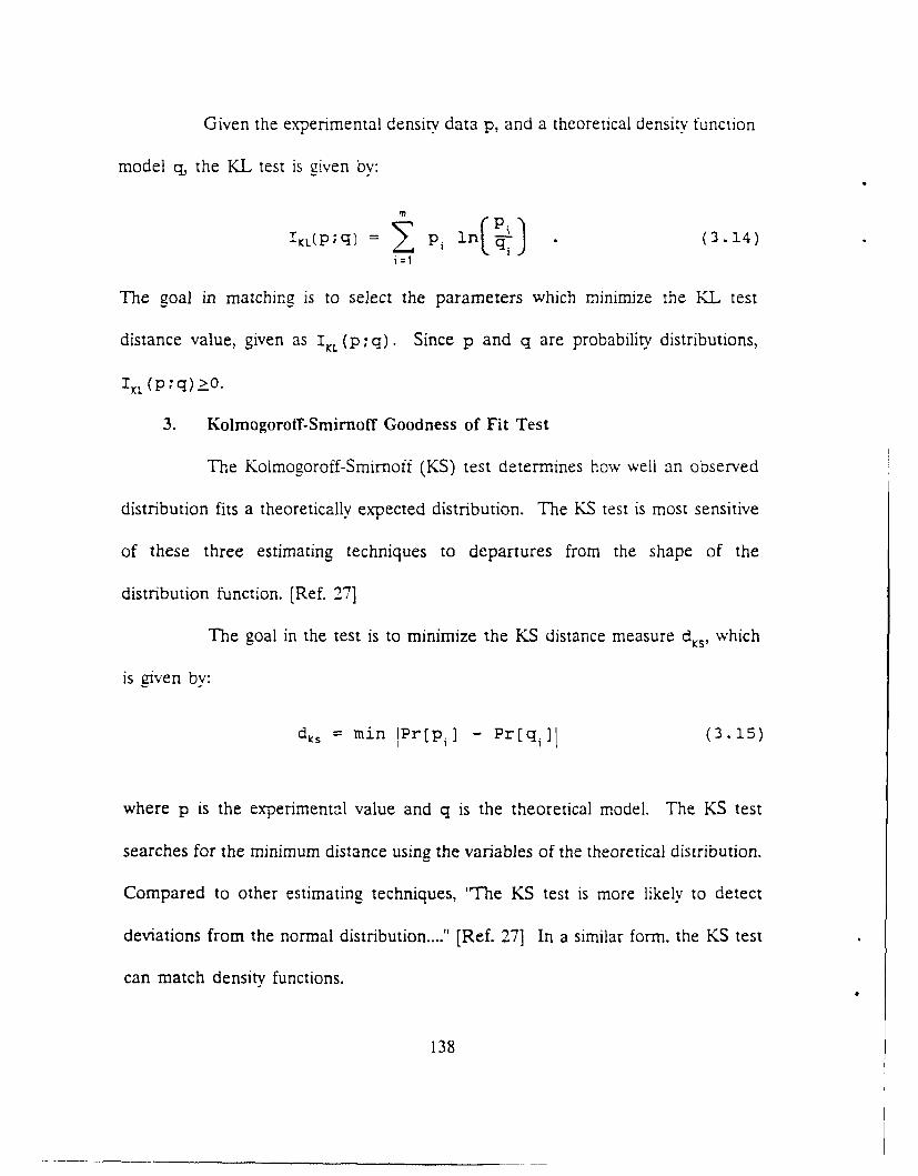
Given the experimental density data p, and a theoretical densitv function
model q, the KL test is given by:
m
IKL(P = P. 1n q (3.14)
The goal in matching is to select the parameters which minimize the KL test
distance value, given as IrL (p; q). Since p and q are probability distributions,
I K (p;q)>O.
3. Kolmogoroff-Smirnoff Goodness of Fit Test
The Kolmogoroff-Smirnoff (KS) test determines how well an observed
distribution fits a theoretically expected distribution. The KS test is most sensitive
of these three estimating techniques to departures from the shape of the
distribution function. [Ref. 271
The goal in the test is to minimize the KS distance measure d K, which
is mven by:
ds = rain lPr[pi] - Pr[q,] (3.15)
where p is the experimental value and q is the theoretical model. The KS test
searches for the minimum distance using the variables of the theoretical distribution.
Compared to other estimating techniques, "The KS test is more likely to detect
deviations from the normal distribution ...." [Ref. 27] In a similar form. the KS test
can match density functions.
138

D. MATCHED LOG-NORMAL DISTRIBUTIONS
Most of the published HF signal observations are in distributional form. The
KS test is the best of the three methods to estimate the means and variances for
matching theoretical distributions. The actual matching is done in the dBm domain.
This results in the process of matching a normal distribution to the experimental
distributions.
Figure 3.9 is a scatter plot of the means and variances used to match normal
distributions to the distributions shown in Figure 3.8. The means cluster around the
-100 to -120 dBm (with some higher), but the variance is widely scattered.
C L'TT 1:5S B-fEB-90
4- Rot.A
+ * Ref. Is
--+ R o t . 1 97 Rf. 20
Rat. 210 Rl. 2
4
E 2S 7
0 7I
0 200 400 600Variance
Figure 3.9 - Mean and Variance Matches Using the KS-Test
139

Most of the observations include day and night measurements. One should
expect a smaller daytime mean and a larger nighttime mean and variance.
One can define a dynamic range requirement as the one percent to the 99
percent points on the distribution. Figure 3.10 is an example distribution using a
-110 dBm mean and a variance of 100. This distribution leads to a design dynamic
range of about 55 dB, and it shows the relatively small dynamic range of the
received signals when one considers only signals of military interest.
C LOTT 1:5'4 6-FE'-90- ,II i
ccv 0
LI,
.0
C N
-140 -120 -100 B -00 -0S~g~iLael(dBm)
Figure 3.10 - Example Signal-of-interest Distribution
140

LIST OF REFERENCES
1. SPAWAR Instruction 0101, 108A; Naval Shore Electronics Criteria, October 1989.
2. Vincent, Wilbur Ray, Jauregui, Stephen, and Adler, Richard W., Training Manual890110-1, A SNEP Team Training Manual (Draft), May 1989.
3. Lott, Gus K. Jr., High Frequency (F') Radio Signal Amplitude Characteristics,HF Receiver Site Performance Criteria, and Expanding The Dynamic Range of HFDigital New Energy Receivers By Strong Signal Elimination, Doctoral Dissertation,Naval Postgraduate School, Monterey, California, June 1990.
4. Couch, Leon W., Digital and Analog Communication Systems, Third Edition,Macmillan Publishing Company, New York, 1990.
5. Delfm Systems DN-91-214, Operators Manual for the Advanced PROPHETSystem, IWG Corporation, San Diego, California, 1991.
6. Vincent, Wilbur Ray, Adler, Richard W., Wadsworth, Donald V.Z., and others,"Quick-Look Report on SNEP Team Visit to NSGA Sabana Seca, PR.," Signal-to-Noise Enhancement Program, December 1991.
7. Cummins. Eugene Joseph Jr., High Frequency Radio Interference, Master'sThesis, Naval Postgraduate School, Monterey, California, March 1979.
8. Harthcock, Clyde T., An Examination of the Radio Frequency Switching Matrixat U.S. Army Field Station Augsburg. U.S. Army Field Station Berlin, and U.S.Naval Security Group Activity Edzell, Master's Thesis, Naval Postgraduate School,Monterey, California, September 1989.
9. 3-D Visions Corporation, GRAFTOOL User's Guide, Torrence, California. 1987-1990.
141

BIBLIOGRAPHY
Vincent. Wilbur Ray, and Jaurequi, Stephen. Technical Note 881115-1, Description ofthe Site Performance Problem, Monterey, California, November 1988.
Vincent. Wilbur Ray, Adler, Richard W., Wadsworth, Donald V.Z., and others, "Quick-Look Report on SNEP Team Visit to NSGA Edzell," Signal-to-Noise EnhancementProgram, December 1991.
142

INITIAL DISTRIBUTION LIST
1. Defense Technical Information Center 2Cameron StationAlexandria, VA 22304-6145
2. Library, Code 52 2Naval Postgraduate SchoolMonterey, CA 93943-5002
3. Chairman, Code ECDepartment of Electrical and Computer EngineeringNaval Postgraduate SchoolMonterey, CA 93943-5000
4. Professor D. V. Wadsworth, Code EC/EdDepartment of Electrical and Computer EngineeringNaval Postgraduate SchoolMonterey, CA 93943-5000
5. Professor R. Adler, Code EC/AbDepartment of Electrical and Computer EngineeringNaval Postgraduate SchoolMonterey, CA 93943-5000
6. Professor W. R. Vincent, Code EC/JaDepartment of Electrical and Computer EngineeringNaval Postgraduate SchoolMonterey, CA 93943-5000
7. CommanderNaval Security Group CommandAttn: G403801 Nebraska Avenue, N.W.Washington, DC 20390
143

8. CommanderNaval Security Group CommandAttn: G4333801 Nebraska Avenue, N.W.Washington. DC 20390
9. CommanderNaval Security Group CommandAttn: G803801 Nebraska Avenue, N.W.Washington, DC 20390
10. ComnanderNaval Security Group CommandAttn: G813801 Nebraska Avenue, N.W.Washington, DC 20390
11. CommanderNaval Electronic Systems Security Engineering CenterAttn: Code 0423801 Nebraska Avenue, N.W.Washington, DC 20390
12. DirectorNational Security AgencyAttn: R6Ft. George G. Meade, MD 20755
144


