
NAVAL POSTGRADUATE SCHOOL Monterey, California
THESIS
Approved for public release; distribution is unlimited
ANALYSIS OF LOW PROBABILITY OF INTERCEPT (LPI) RADAR SIGNALS USING CYCLOSTATIONARY PROCESSING
by
Antonio F. Lima, Jr.
September 2002
Thesis Advisor: Phillip E. Pace Thesis Co-Advisor: Herschel H. Loomis

THIS PAGE INTENTIONALLY LEFT BLANK

i
REPORT DOCUMENTATION PAGE Form Approved OMB No. 0704-0188 Public reporting burden for this collection of information is estimated to average 1 hour per response, including the time for reviewing instruction, searching existing data sources, gathering and maintaining the data needed, and completing and reviewing the collection of information. Send comments regarding this burden estimate or any other aspect of this collection of information, including suggestions for reducing this burden, to Washington headquarters Services, Directorate for Information Operations and Reports, 1215 Jefferson Davis Highway, Suite 1204, Arlington, VA 22202-4302, and to the Office of Management and Budget, Paperwork Reduction Project (0704-0188) Washington DC 20503. 1. AGENCY USE ONLY (Leave blank)
2. REPORT DATE September 2002
3. REPORT TYPE AND DATES COVERED Master’s Thesis
4. TITLE AND SUBTITLE: Analysis of Low Probability of Intercept (LPI) Radar Signals Using Cyclostationary Processing
6. AUTHOR(S) Antonio F. Lima, Jr.
5. FUNDING NUMBERS
7. PERFORMING ORGANIZATION NAME(S) AND ADDRESS(ES) Naval Postgraduate School Monterey, CA 93943-5000
8. PERFORMING ORGANIZATION REPORT NUMBER
9. SPONSORING /MONITORING AGENCY NAME(S) AND ADDRESS(ES) Office of Naval Research
10. SPONSORING/MONITORING AGENCY REPORT NUMBER
11. SUPPLEMENTARY NOTES The views expressed in this thesis are those of the author and do not reflect the official policy or position of the Department of Defense or the U.S. Government. 12a. DISTRIBUTION / AVAILABILITY STATEMENT Distribution unlimited.
12b. DISTRIBUTION CODE
13. ABSTRACT (maximum 200 words) LPI radar is a class of radar systems possessing certain performance characteristics that make them nearly undetectable by today’s digital intercept receivers. This presents a significant tactical problem in the battle space. To detect these types of radar, new digital receivers that use sophisticated signal processing techniques are required. This thesis investigates the use of cyclostationary processing to extract the modulation parameters from a variety of continuous-wave (CW) low-probability-of-intercept (LPI) radar waveforms. The cyclostationary detection techniques described exploit the fact that digital signals vary in time with single or multiple periodicity, owing to their spectral correlation, namely non-zero correlation between certain frequency components, at certain frequency shifts. The use of cyclostationary signal processing in a non-cooperative intercept receiver can help identify the particular emitter and aid in the development of electronic attack signals. LPI CW waveforms examined include Frank codes, P1 through P4, Frequency Modulated CW (FMCW), Costas frequencies as well as several frequency-shift-keying/phase-shift-keying (FSK/PSK) waveforms. This thesis show that for signal-to-noise ratios of 0 dB and –6 dB, the cyclostationary signal processing can extract the modulation parameters necessary in order to distinguish between the various types of LPI modulations.
NUMBER OF PAGES 186
14. SUBJECT TERMS Low Probability of Intercept (LPI) Radars, Electronic Support Measures (ESM), FFT Accumulation Method (FAM), Direct Frequency Smoothing Method (DFSM), Binary Phase Shift Keying (BPSK), Frequency Modulated Continuous Wave (FMCW), Polyphase Codes (P4, P3, P2, P1 and Frank Codes), Combined FSK/PSK (Frequency Shift Keying and Phase Shift Keying) 16. PRICE CODE
17. SECURITY CLASSIFICATION OF REPORT
Unclassified
18. SECURITY CLASSIFICATION OF THIS PAGE
Unclassified
19. SECURITY CLASSIFICATION OF ABSTRACT
Unclassified
20. LIMITATION OF ABSTRACT
UL
NSN 7540-01-280-5500 Standard Form 298 (Rev. 2-89) Prescribed by ANSI Std. 239-18

ii
THIS PAGE INTENTIONALLY LEFT BLANK

iii
Approved for public release; distribution is unlimited.
ANALYSIS OF LOW PROBABILITY OF INTERCEPT (LPI) RADAR SIGNALS USING CYCLOSTATIONARY PROCESSING
Antonio F. Lima, Jr.
Captain, Brazilian Air Force B.S., Brazilian Air Force Academy, Brazil
Submitted in partial fulfillment of the requirements for the degree of
MASTER OF SCIENCE IN SYSTEMS ENGINEERING
from the
NAVAL POSTGRADUATE SCHOOL September 2002
Author: Antonio F. Lima, Jr.
Approved by: Phillip E. Pace
Thesis Advisor
Herschel H. Loomis Thesis Co-Advisor
Dan C. Boger Chairman, Information Sciences Department

iv
THIS PAGE INTENTIONALLY LEFT BLANK
v
ABSTRACT LPI radar is a class of radar systems that possess certain performance
characteristics that make them nearly undetectable by today’s digital intercept receivers.
This presents a significant tactical problem in the battle space. To detect these types of
radar, new digital receivers that use sophisticated signal processing techniques are
required.
This thesis investigates the use of cyclostationary processing to extract the
modulation parameters from a variety of continuous-wave (CW) low-probability-of-
intercept (LPI) radar waveforms. The cyclostationary detection techniques described
exploit the fact that digital signals vary in time with single or multiple periodicities,
because they have spectral correlation, namely, non-zero correlation between certain
frequency components, at certain frequency shifts. The use of cyclostationary signal
processing in a non-cooperative intercept receiver can help identify the particular emitter
and can help develop electronic attacks. LPI CW waveforms examined include Frank
codes, polyphase codes (P1 through P4), Frequency Modulated CW (FMCW), Costas
frequencies as well as several frequency-shift-keying/phase-shift-keying (FSK/PSK)
waveforms. It is shown that for signal-to-noise ratios of 0dB and –6 dB, the
cyclostationary signal processing can extract the modulation parameters necessary in
order to distinguish among the various types of LPI modulations.

vi
THIS PAGE INTENTIONALLY LEFT BLANK
vii
TABLE OF CONTENTS
I. INTRODUCTION........................................................................................................1 A. LPI RADARS ...................................................................................................1 B. PRINCIPAL CONTRIBUTIONS ..................................................................2 C. THESIS OUTLINES .......................................................................................3
II. LPI WAVEFORMS DESCRIPTION ........................................................................5 A. BACKGROUND ..............................................................................................5 B. FSK/PSK COMBINED USING A COSTAS-BASED FREQUENCY-
HOPPING (FH) TECHNIQUE ......................................................................6 C. FSK/ PSK COMBINED USING A TARGET-MATCHED
FREQUENCY HOPPING.............................................................................15
III. CYCLOSTATIONARY SIGNAL PROCESSING ALGORITHMS AND TUTORIAL ................................................................................................................21 A. CYCLOSTATIONARY THEORY ..............................................................21 B. DISCRETE TIME CYCLOSTATIONARY ALGORITHMS ..................27
1. The Time-Smoothing FFT Accumulation Method (FAM): ...........27 2. Direct Frequency-Smoothing Method: ............................................31 3. GUI Implementation: ........................................................................33
C. PROCESSING TUTORIAL .........................................................................35 1. Test Signals:........................................................................................35 2. BPSK:..................................................................................................37 3. FMCW: ...............................................................................................40 4. P4:........................................................................................................43
C. CHAPTER SUMMARY................................................................................46
IV. DESCRIPTION OF LPI SPECTRAL PROPERTIES AND CYCLOSTATIONARY PROCESSING RESULTS ..............................................47 A. TEST SIGNALS.............................................................................................48
1. Description..........................................................................................48 2. Spectral Properties and Results (T_1_7_1_s and T_12_7_2_s) .....48
B. BPSK ...............................................................................................................50 1. Description: ........................................................................................50 2. Spectral Properties and Results (B_1_7_7_1_s)..............................51
C. FMCW ............................................................................................................59 1. Description..........................................................................................59 2. Spectral Properties and Results (F_1_7_250_20_s) ........................60
D. P1 .....................................................................................................................68 1. Description..........................................................................................68 2. Spectral Properties and Results (P1_1_7_16_1_s) ..........................69
E. P2 .....................................................................................................................75 1. Description..........................................................................................75 2. Spectral Properties and Results (P2_1_7_16_1_s) ..........................76
viii
F. P3 .....................................................................................................................81 2. Spectral Properties and Results (P3_1_7_16_1_s) ..........................82
G. P4 .....................................................................................................................89 2. Spectral Properties and Results (P4_1_7_16_1_s) ..........................90
H. FRANK ...........................................................................................................96 2. Spectral Properties and Results (FR_1_7_16_1_s) .........................97
I. COSTAS CODES.........................................................................................104 1. Description........................................................................................104 2. Spectral Properties and Results (C_1_15_10_s)............................104
J. FSK/ PSK COSTAS.....................................................................................109 1. Description........................................................................................109 2. Spectral Properties and Results (FSK_PSK_C_1_15_5_1_s) ......109
K. FSK/ PSK TARGET....................................................................................116 1. Description........................................................................................116 2. Spectral Properties and Results (FSK_PSK_T_15_128_5_s) ......116
L. COMPARISON BETWEEN POLYPHASE CODES ..............................120 M. CHAPTER SUMMARY..............................................................................123
V. CONCLUSIONS AND RECOMMENDATIONS.................................................125
APPENDIX A. CYCLOSTATIONARY IMPLEMENTATION CODES (CYCLO.M, FAM.M AND DFSM.M)...................................................................127
APPENDIX B. FSK/PSK GENERATION CODES................................................137
APPENDIX C. LIST OF LPI RADAR SIGNALS ANALYZED...........................155
LIST OF REFERENCES....................................................................................................159

ix
LIST OF FIGURES
Figure 1 a) FSK/PSK Costas LPI Generator MATLAB® [4] code block diagram and, b) general FSK/PSK signal containing NF frequency hops with NP phase slots per frequency. ..................................................................................7
Figure 2 PSD plot for a Costas FH waveform with no phase modulation. ......................8 Figure 3 Time domain plot for a Costas FH waveform with no phase modulation. ........9 Figure 4 PSD for FSK/PSK Costas FH phase modulated with a Barker-11 sequence
and 1 cpp. .........................................................................................................10 Figure 5 Phase plot for FSK/PSK Costas FH phase modulated with a Barker-11
sequence...........................................................................................................11 Figure 6 PAF contour plot for FSK/PSK Costas FH phase modulated with a
Barker-11 sequence (plot of one period for all frequencies in one Costas sequence)..........................................................................................................11
Figure 7 PAF delay axis cut for FSK/PSK Costas FH phase modulated with a Barker-11 sequence (plot of one period for all frequencies in one Costas sequence)..........................................................................................................12
Figure 8 PAF Doppler axis cut for FSK/PSK Costas FH phase modulated with a Barker-11 sequence (plot of one period for all frequencies in one Costas sequence)..........................................................................................................12
Figure 9 PAF contour plot for FSK/PSK Costas FH phase modulated with a Barker-11 sequence (plot of one period for one frequency in the Costas sequence)..........................................................................................................13
Figure 10 PAF delay axis cut for FSK/PSK Costas FH phase modulated with a Barker-11 sequence (plot of one period for one frequency in the Costas sequence)..........................................................................................................14
Figure 11 PAF Doppler axis cut for FSK/PSK Costas FH phase modulated with a Barker-11 sequence (plot of one period for one frequency in the Costas sequence)..........................................................................................................14
Figure 12 Block diagram of the MATLAB® [4] implementation of FSK/PSK target matched waveform...........................................................................................16
Figure 13 FSK/PSK target 64 complex points radar range simulated response. .............17 Figure 14 FSK/PSK target frequency probability distribution of 64 frequency
components. .....................................................................................................17 Figure 15 FSK/PSK target 64 frequency components histogram with number of
occurrences per frequency for 256 frequency hops. ........................................18 Figure 16 PSD for FSK/PSK target with 64 frequency components, 256 frequency
hops, random phase modulation and 5 cpp. .....................................................18 Figure 17 PAF contour plot for FSK/PSK target with 64 frequency components, 256
frequency hops, random phase modulation and 5 cpp. ....................................19 Figure 18 PAF delay cut for FSK/PSK target with 64 frequency components, 256
frequency hops, random phase modulation and 5 cpp. ....................................19

x
Figure 19 PAF Doppler cut for FSK/PSK target with 64 frequency components, 256 frequency hops, random phase modulation and 5 cpp. ....................................20
Figure 20 Pictorial illustration of the estimation of the time-variant spectral periodogram (adapted from [12, 17])...............................................................24
Figure 21 Sequence of frequency products for each short-time Fourier transforms (adapted from [12, 17]). ...................................................................................25
Figure 22 Bi-frequency plane, frequency and cycle frequency resolutions on detailed area (adapted from [12, 17]). ...........................................................................26
Figure 23 FAM block diagram (adapted from [3, 13]). ...................................................28 Figure 24 Division of bi-frequency plane in channel pair regions (adapted from [3,
15]). ..................................................................................................................29 Figure 25 Cycle frequency and frequency resolutions and the Grenander’s
Uncertainty Condition (adapted from [3, 13]). ................................................30 Figure 26 DFSM algorithm block diagram (adapted from [3, 13])..................................32 Figure 27 Cyclostationary processing GUI schematic tutorial. .......................................33 Figure 28 DFSM generated SCD bi-frequency for a test signal (1000Hz single
carrier)..............................................................................................................36 Figure 29 FAM generated SCD bi-frequency for a test signal (1000Hz single
carrier)..............................................................................................................36 Figure 30 Pictorial generic illustration of a BPSK signal SCD result..............................37 Figure 31 Zoomed in pictorial generic illustration of a BPSK signal SCD result with
estimation of BW, number of phases and code rate.........................................38 Figure 32 DFSM generated SCD plot for a BPSK signal (1000Hz single carrier and
11 bits Barker-code phase modulation) with estimated BW. ..........................39 Figure 33 Zoomed-in DFSM generated SCD plot for a BPSK signal (estimated code
rate measurement). ...........................................................................................39 Figure 34 Pictorial generic illustration of a FMCW signal SCD result. ..........................41 Figure 35 Pictorial generic illustration of a zoomed-in plot for a FCMW signal SCD. ..41 Figure 36 FAM generated SCD plot for a FMCW signal (1000Hz carrier and
estimated modulation BW of 230 Hz). ............................................................42 Figure 37 Zoomed-in FAM generated SCD plot for a FMCW signal (“delta” value
of 25Hz). ..........................................................................................................43 Figure 38 FAM-generated SCD plot for a P4 signal (1125Hz carrier and estimated
BW of 1000Hz). ...............................................................................................44 Figure 39 Zoomed-in FAM-generated SCD plot for a P4 signal (with estimated code
rate (fb) of 66Hz). .............................................................................................44 Figure 40 Zoomed-in FAM-generated SCD plot for a P4 signal (with estimation of
BW and number of phases)..............................................................................45 Figure 41 PSD plots for both Test signals: a) 1000Hz single sarrier and b) 1 and
2000Hz double carrier, no modulation. ...........................................................48 Figure 42 DFSM generated estimated SCD for a Test signal (1000Hz and 2000Hz
double carrier)..................................................................................................49 Figure 43 Zoomed in DFSM generated estimated SCD for a Test signal (1000 and
2000Hz double carrier). ...................................................................................49 Figure 44 Block diagram for BPSK modulation (from [5]). ............................................51

xi
Figure 45 PSD for a Barker signal (1000Hz carrier, 7-bits Barker sequence and 1 NPBB). .............................................................................................................52
Figure 46 Estimated FAM SCD contour plot for a BPSK real signal with 1000Hz carrier, Barker-7 code and 1 NPBB..................................................................52
Figure 47 Estimated FAM SCD contour plot for a BPSK real signal with 1000Hz carrier, Barker-7 code and 1 NPBB, with estimated carrier of 1000Hz and estimated BW of 1000Hz.................................................................................53
Figure 48 Zoomed-in FAM SCD contour plot for a BPSK signal with 1000Hz carrier, Barker-7 code and 1 NPBB, with estimated bf of 141 Hz..................53
Figure 49 Estimated DFSM SCD contour plot for a BPSK signal with 1000Hz carrier, Barker-7 code and 1 NPBB, with estimated BW of 1000Hz...............54
Figure 50 Zoomed-in estimated DFSM SCD contour plot for a BPSK signal with 1000Hz carrier, Barker-7 code and NPBB = 1, with estimated bf of 142Hz...............................................................................................................54
Figure 51 PSD for a Barker signal (1000Hz carrier, 7-bits Barker sequence, 1 NPBB and 0 dB SNR). ................................................................................................55
Figure 52 Estimated FAM SCD contour plot for a BPSK signal with 1000Hz carrier, 7-bits Barker code, 1 NPBB and 0 dB SNR, with estimated BW of 1000Hz.............................................................................................................55
Figure 53 Zoomed-in estimated FAM SCD for BPSK with 1000Hz carrier, Barker-7 code, 1 NPBB, 0 dB SNR, with estimated bf of 143Hz..................................56
Figure 54 Estimated DFSM SCD for BPSK with 1000Hz carrier, Barker-7 code, 1 NPBB, 0 dB SNR, with estimated BW of 1000Hz. .........................................56
Figure 55 Zoomed-in estimated FAM SCD for BPSK with 1000Hz carrier, Barker-7 code, 1 NPBB, 0 dB SNR, with estimated bf of 144Hz..................................57
Figure 56 Graphic demonstration of detection effectiveness for the BPSK modulation. ......................................................................................................58
Figure 57 Linear Frequency Modulated Triangular Waveform and Doppler Shifted Signal [5]..........................................................................................................59
Figure 58 PSD for an FMCW signal (1000Hz carrier, 250Hz modulation BW and 20ms modulation period, only signal). ............................................................61
Figure 59 Time X Frequency plot for an FMCW signal (20ms triangular modulation up-ramp period). ..............................................................................................61
Figure 60 Estimated FAM SCD contour plot for an FMCW signal with 1000Hz carrier and estimated modulation BW of 230Hz. ............................................62
Figure 61 Zoomed-in estimated FAM SCD contour plot for an FMCW signal with an estimated “delta” value of 25Hz.................................................................62
Figure 62 Estimated DFSM SCD contour plot for an FMCW signal with 1000Hz carrier and estimated modulation BW of 235Hz. ............................................63
Figure 63 Zoomed-in estimated DFSM SCD contour plot for an FMCW signal with an estimated “delta” value of 21Hz.................................................................63
Figure 64 PSD for an FMCW signal (1000Hz carrier, 250 Hz modulation BW and 20ms modulation period, 0dB SNR)................................................................64

xii
Figure 65 Estimated FAM SCD contour plot for an FMCW signal with 1000Hz carrier, 0 dB SNR and estimated modulation BW of 200 Hz. .........................64
Figure 66 Estimated FAM SCD contour plot for an FMCW signal with an estimated “delta” value of 26Hz. ....................................................................................65
Figure 67 PSD for an FMCW signal (1000Hz carrier, 250 Hz modulation BW and 20ms modulation period, -6dB SNR). .............................................................65
Figure 68 Estimated FAM SCD contour plot for an FMCW signal with 1000Hz carrier, -6 dB SNR and estimated modulation BW of 200 Hz.........................66
Figure 69 Estimated FAM SCD contour plot for an FMCW signal with an estimated “delta” value of 27Hz. ....................................................................................66
Figure 70 Graphic demonstration of detection effectiveness for the FMCW modulation. ......................................................................................................68
Figure 71 P1 code phase shift...........................................................................................69 Figure 72 PSD for a P1 signal (1000Hz carrier, 16 phases and 1 cpp, only signal). .......70 Figure 73 Estimated DFSM SCD contour plot for a P1 signal with 900Hz carrier and
estimated BW of 1000Hz.................................................................................70 Figure 74 Zoomed-in estimated DFSM SCD contour plot for a P1 signal with an
estimated code rate (fb) of 62Hz.......................................................................71 Figure 75 PSD for a P1 signal (1000Hz carrier, 16 phases and 1 cpp, 0dB SNR)...........71 Figure 76 Estimated FAM SCD contour plot for a P1 signal with 900Hz carrier and
estimated BW of 1000Hz, with 0dB SNR. ......................................................72 Figure 77 Zoomed-in estimated FAM SCD contour plot for a P1 signal with an
estimated code rate (fb) of 65Hz, with 0dB SNR. ............................................72 Figure 78 PSD for a P1 signal (1000Hz carrier, 16 phases and 1 cpp, -6dB SNR). ........73 Figure 79 Estimated FAM SCD contour plot for a P1 signal with 850Hz carrier and
estimated BW of 1000Hz, with -6dB SNR......................................................73 Figure 80 Graphic demonstration of detection effectiveness for the P1 modulation.......75 Figure 81 P2 symmetric phase relationship between the index in the matrix and its
phase shift. .......................................................................................................76 Figure 82 PSD for a P2 signal (1000Hz carrier, 16 phases and 1 cpp, only signal). .......77 Figure 83 Estimated FAM SCD contour plot for a P2 signal with 1000Hz carrier and
estimated BW of 950 Hz..................................................................................77 Figure 84 Zoomed-in estimated FAM SCD contour plot for a P2 signal with an
estimated code rate (fb) of 65 Hz......................................................................78 Figure 85 PSD for a P2 signal (1000Hz carrier, 16 phases and 1 cpp, 0dB SNR)...........78 Figure 86 Estimated DSFM SCD contour plot for a P2 signal with 1000Hz carrier
and estimated BW of 850Hz, with 0dB SNR. .................................................79 Figure 87 Zoomed-in estimated DFSM SCD contour plot for a P2 signal with an
estimated code rate (fb) of 65Hz, with 0dB SNR. ............................................79 Figure 88 Graphic demonstration of detection effectiveness for the P2 modulation.......81 Figure 89 P3 code phase shift...........................................................................................82 Figure 90 PSD for a P3 signal (1000Hz carrier, 16 phases and 1 cpp, only signal). .......83 Figure 91 Estimated FAM SCD contour plot for a P3 signal with 1100Hz carrier and
estimated BW of 1000Hz.................................................................................83

xiii
Figure 92 Zoomed-in estimated FAM SCD contour plot for a P3 signal with an estimated fb of 62 Hz........................................................................................84
Figure 93 Estimated DFSM SCD contour plot for a P3 signal with 1150Hz carrier and estimated BW of 1000Hz. .........................................................................84
Figure 94 Zoomed-in estimated FAM SCD contour plot for a P3 signal with an estimated fb of 63 Hz........................................................................................85
Figure 95 PSD for a P3 signal (1000Hz carrier, 16 phases, 1 cpp, and 0dB SNR)..........85 Figure 96 Estimated FAM SCD contour plot for a P3 signal with 1050Hz carrier and
estimated BW of 1000Hz, with 0dB SNR. ......................................................86 Figure 97 Zoomed-in estimated FAM SCD contour plot for a P3 signal with an
estimated fb of 56 Hz and 0dB SNR.................................................................86 Figure 98 Estimated DFSM SCD contour plot for a P3 signal with 1050Hz carrier
and estimated BW of 1000Hz, with 0dB SNR. ...............................................87 Figure 99 Zoomed-in estimated DFSM SCD contour plot for a P3 signal with an
estimated fb of 68 Hz and 0dB SNR.................................................................87 Figure 100 Graphic demonstration of detection effectiveness for the P3 modulation.......89 Figure 101 Phase shift for a P4-coded signal with Np=64 phases .....................................90 Figure 102 PSD for a P4 signal (1000Hz carrier, 16 phases and 1 cpp, only signal). .......91 Figure 103 Estimated FAM SCD contour plot for a P4 signal with 1100Hz carrier and
estimated BW of 1000 Hz................................................................................91 Figure 104 Zoomed-in estimated FAM SCD contour plot for a P4 signal with an
estimated bf of 66 Hz......................................................................................92 Figure 105 Estimated DFSM SCD contour plot for a P4 signal with 1100Hz carrier
and estimated BW of 1000 Hz. ........................................................................92 Figure 106 Zoomed-in estimated FAM SCD contour plot for a P4 signal with an
estimated bf of 62 Hz......................................................................................93 Figure 107 PSD for a P4 signal (1000Hz carrier, 16 phases, 1 cpp, and 0dB SNR)..........93 Figure 108 Estimated FAM SCD contour plot for a P4 signal with 1100Hz carrier and
estimated BW of 1000 Hz, with 0dB SNR. .....................................................94 Figure 109 Zoomed-in estimated FAM SCD contour plot for a P4 signal with an
estimated bf of 67 Hz, with 0dB SNR. ...........................................................94 Figure 110 Graphic demonstration of detection effectiveness for the P4 modulation.......96 Figure 111 Frank modulation phase changes Np2=16........................................................97 Figure 112 PSD for a Frank signal (1000Hz carrier, 16 phases and 1 cpp, only signal). ..98 Figure 113 Estimated DFSM SCD contour plot for a Frank signal with 1150Hz carrier
and estimated BW of 1000 Hz. ........................................................................98 Figure 114 Zoomed-in estimated DFSM SCD contour plot for a Frank signal with an
estimated fb of 61 Hz........................................................................................99 Figure 115 PSD for a Frank signal (1000Hz carrier, 16 phases, 1 cpp, and 0dB SNR). ...99 Figure 116 Estimated FAM SCD contour plot for a Frank signal with 1000Hz carrier
and estimated BW of 1000 Hz, with 0dB SNR. ............................................100 Figure 117 Zoomed-in estimated FAM SCD contour plot for a Frank signal with an
estimated fb of 63 Hz and 0dB SNR...............................................................100 Figure 118 PSD for a Frank signal (1000Hz carrier, 16 phases, 1 cpp, and -6dB SNR). 101
xiv
Figure 119 Estimated FAM SCD contour plot for a Frank signal with 1100Hz carrier and estimated BW of 1000 Hz, with -6dB SNR. ...........................................101
Figure 120 Zoomed-in estimated FAM SCD contour plot for a Frank signal with an estimated fb of 65 Hz, and –6dB SNR............................................................102
Figure 121 Graphic demonstration of detection effectiveness for the Frank modulation. ....................................................................................................103
Figure 122 PSD for a Costas signal (1, 2, 3, 4, 5, 6 and 7 kHz carriers, 10 cpf, only signal).............................................................................................................105
Figure 123 Estimated FAM SCD contour plot for a complex Costas signal (1, 2, 3, 4, 5, 6 and 7000Hz carriers over 0γ = axis, cpf=10, only signal), with intermodulation products. ..............................................................................105
Figure 124 PSD for a Costas signal (1, 2, 3, 4, 5, 6 and 7kHz carriers, 10 cpf and 0dB SNR). .............................................................................................................106
Figure 125 Estimated FAM SCD contour plot for a complex Costas signal (1, 2, 3, 4, 5, 6 and 7kHz carriers over 0γ = axis, 10 cpf, 0dB SNR), with intermodulation products. ..............................................................................106
Figure 126 PSD for a Costas signal (1, 2, 3, 4, 5, 6 and 7kHz carriers, 10 cpf and SNR of -6dB)..........................................................................................................107
Figure 127 Estimated FAM SCD contour plot for a complex Costas signal (1, 2, 3, 4, 5, 6 and 7kHz carriers over 0γ = axis, 10 cpf, -6dB SNR), with intermodulation products. ..............................................................................107
Figure 128 Graphic demonstration of detection effectiveness for the Costas modulation. ....................................................................................................109
Figure 129 PSD for a FSK/PSK Costas signal (1, 2, 3, 4, 5, 6 and 7kHz carriers, Barker-5 and 1 NPBB, only signal)................................................................110
Figure 130 Barker-5 phase sequence used inside each hop. ............................................110 Figure 131 Estimated FAM SCD contour plot for a complex FSK/PSK Costas signal
(1, 2, 4, 5, 6 and 7kHz measured carriers). ....................................................111 Figure 132 Zoomed-in estimated FAM SCD contour plot for a complex FSK/PSK
Costas signal (4, 5 and 6kHz measured carriers and estimated BW of 1000 Hz for each frequency hop)............................................................................111
Figure 133 Estimated fb value of 200 Hz for the embedded Barker-5 BPSK modulation. ....................................................................................................112
Figure 134 PSD for a FSK/PSK Costas signal (1, 2, 3, 4, 5, 6 and 7kHz carriers, Barker-5 and 1 NPBB, 0dB SNR). ................................................................112
Figure 135 Estimated FAM SCD contour plot for a complex FSK/PSK Costas signal (1, 2, 4, 5, 6 and 7kHz measured carriers, 0dB SNR)....................................113
Figure 136 Zoomed-in estimated FAM SCD contour plot for a complex FSK/PSK Costas signal (5, 6 and 7kHz measured carriers and estimated BW of 1000 Hz for each frequency hop, 0dB SNR). .........................................................113
Figure 137 Estimated fb value of 200 Hz for the embedded Barker-5 BPSK modulation. ....................................................................................................114
Figure 138 Graphic demonstration of detection effectiveness for the FSK/PSK Costas modulation. ....................................................................................................116

xv
Figure 139 PSD for a FSK/PSK Target signal (4200Hz BW, random phase with length 5 and 5 cpp, only signal). ....................................................................117
Figure 140 Random phase sequence of length 5 used inside each hop............................117 Figure 141 Frequency hops histogram after random firing order generator. ...................118 Figure 142 Estimated FAM SCD contour plot for a complex FSK/PSK Target signal
with an estimated BW of 4800Hz..................................................................118 Figure 143 Graphic demonstration of detection effectiveness for the FSK/PSK Target
modulation. ....................................................................................................120 Figure 144 Estimated DFSM SCD contour plot for a Frank signal with 1150Hz
carrier, BW of 1000 Hz, Np2=16 and cpp=1..................................................121 Figure 145 Estimated DFSM SCD contour plot for a P1 signal with 900Hz carrier,
BW of 1000 Hz, Np2=16 and cpp=1. .............................................................121 Figure 146 Estimated DFSM SCD contour plot for a P2 signal with 1050Hz carrier,
BW of 950 Hz, Np2=16 and cpp=1. ...............................................................122 Figure 147 Estimated DFSM SCD contour plot for a P3 signal with 1150Hz carrier,
BW of 1000 Hz, Np=16 and cpp=1. ..............................................................122 Figure 148 Estimated DFSM SCD contour plot for a P4 signal with 1150Hz carrier,
BW of 1000 Hz, Np=16 and cpp=1. ..............................................................123

xvi
THIS PAGE INTENTIONALLY LEFT BLANK

xvii
LIST OF TABLES
Table 1. Comparison of the estimated time-smoothed Periodogram expressed in continuous and discrete time............................................................................28
Table 2. Recommended variables values for GUI users................................................34 Table 3. Test signal characteristics. ...............................................................................35 Table 4. BPSK signal characteristics. ............................................................................37 Table 5. FMCW signal characteristics...........................................................................40 Table 6. P4 signals characteristics. ................................................................................43 Table 7. List of signal examples analyzed in this thesis. ...............................................47 Table 8. Comparison between measured and original characteristics for the Test
signals. .............................................................................................................50 Table 9. B_1_7_7_1_s signal characteristics.................................................................51 Table 10. Comparison between measured and original characteristics for This BPSK
signal. ...............................................................................................................57 Table 11. Summary of all measurements for the BPSK modulation. ..............................58 Table 12. Detection effectiveness for the BPSK modulation. .........................................58 Table 13. F_1_7_250_20_s signal characteristics. ..........................................................60 Table 14. Comparison between measured and original characteristics for an FMCW
signal. ...............................................................................................................67 Table 15. Summary of all measurements for the FMCW modulation.............................67 Table 16. Detection effectiveness for the FMCW modulation. .......................................67 Table 17. P1_1_7_16_1_s signal characteristics. ............................................................69 Table 18. Comparison between measured and original characteristics for a P1 signal. ..74 Table 19. Summary of all measurements for the P1 modulation.....................................74 Table 20. Detection effectiveness for the P1 modulation. ...............................................75 Table 21. P2_1_7_16_1_s signal characteristics. ............................................................76 Table 22. Comparison between measured and original characteristics for a P2 signal. ..80 Table 23. Summary of all measurements for the P2 modulation.....................................80 Table 24. Detection effectiveness for the P2 modulation. ...............................................80 Table 25. P3_1_7_16_1_s Signal characteristics.............................................................82 Table 26. Comparison between measured and original characteristics for a P3 signal. ..88 Table 27. Summary of all measurements for the P3 modulation.....................................88 Table 28. Detection effectiveness for the P3 modulation. ...............................................88 Table 29. P4_1_7_16_1_s signal characteristics. ............................................................90 Table 30. Comparison between measured and original characteristics for a P4 signal. ..95 Table 31. Summary of all measurements for the P4 modulation.....................................95 Table 32. Detection effectiveness for the P4 modulation. ...............................................95 Table 33. FR_1_7_16_1_s signal characteristics.............................................................97 Table 34. Comparison between measured and original characteristics for a Frank
signal. .............................................................................................................102 Table 35. Summary of all measurements for the Frank modulation..............................103 Table 36. Detection effectiveness for the Frank modulation. ........................................103

xviii
Table 37. C_1_15_10_s signal characteristics...............................................................104 Table 38. Comparison between measured and original characteristics for a Costas
signal. .............................................................................................................108 Table 39. Summary of all measurements for the Costas modulation. ...........................108 Table 40. Detection effectiveness for the Costas modulation........................................108 Table 41. FSK_PSK_C_1_15_5_1_s signal characteristics. .........................................109 Table 42. Comparison between measured and original characteristics for a FSK/PSK
Costas signal. .................................................................................................114 Table 43. Summary of all measurements for the FSK/PSK Costas modulation............115 Table 44. Detection effectiveness for the FSK/PSK Costas modulation.......................115 Table 45. FSK_PSK_T_15_128_5_s Signal characteristics..........................................116 Table 46. Comparison between measured and original characteristics for a FSK/PSK
Target signal...................................................................................................119 Table 47. Summary of all measurements for the FSK/PSK Target modulation............119 Table 48. Detection effectiveness for the FSK/PSK Target modulation. ......................120 Table 49. Test matrix of LPI radar signals analyzed. ....................................................155 Table 50. Test matrix of LPI radar signals analyzed. ....................................................156 Table 51. Test matrix of LPI radar signals analyzed. ....................................................157

xix
ACKNOWLEDGMENTS
I would like to thank Professor Phillip E. Pace and Professor Herschel H. Loomis
for their constant guidance, support and patience during this research effort. I am also
thankful for the very carefully conducted editing work of Professor Roy R. Russell.
I address special thanks to all my superiors of the Brazilian Air Force, COL
Narcelio Ramos Ribeiro and Officers of the General Air Command Electronic Warfare
Center (CGEGAR), and Dr. Jose Edimar Barbosa of the Aeronautics Institute of
Technology (ITA) for their vision and support in making my study at the Naval
Postgraduate School possible.
I would also like to thank my wife, Luciana, and my daughter, Marina, for their
unconditional love, support, and understanding throughout our entire stay here in the
United States and especially thank them for all the time I had to spend away from them in
order to accomplish this work.

xx
THIS PAGE INTENTIONALLY LEFT BLANK

xxi
EXECUTIVE SUMMARY
LPI radar is a class of radar systems possessing certain performance
characteristics that make today’s digital intercept receivers virtually unable to detect
them. This presents a significant tactical problem in the battle space. To detect these
types of radar, the military requires new digital receivers that use sophisticated signal
processing techniques.
This thesis investigates the use of cyclostationary processing to extract the
modulation parameters from a variety of continuous-wave (CW) low-probability-of-
intercept (LPI) radar waveforms. The cyclostationary detection techniques described
exploit the fact that digital signals vary in time with single or multiple periodicity, owing
to their spectral correlation, namely, non-zero correlation between certain frequency
components, at certain frequency shifts. The use of cyclostationary signal processing in a
non-cooperative intercept receiver can help identify the particular emitter and can help
develop electronic attacks. LPI CW waveforms examined include Frank codes, polyphase
codes (P1, P2, P3 and P4), Frequency Modulated CW (FMCW), Costas frequencies as
well as several frequency-shift-keying/phase-shift-keying (FSK/PSK) waveforms. This
thesis shows that for signal-to-noise ratios of 0dB and –6 dB, the cyclostationary signal
processing can extract modulation parameters such as carrier frequency, chip rate, code
rate and bandwidth, necessary in order to distinguish between the various types of LPI
radar modulations.
Two computationally efficient methods of cyclostationary processing were
implemented: Time Smoothing FFT Accumulation and Direct Frequency Smoothing. It is
possible to verify that the time smoothing method is more computationally efficient than
the frequency smoothing for signals with higher complexity (polyphase codes, Frank
codes, Costas and FSK/PSK). The results from both methods were compared and
discussed for various LPI modulation types.
The results due to variations of modulation characteristics are compared and the
efficiency of both cyclostationary methods for each modulation is measured with relation

xxii
to the original parameters. This thesis also includes comments on which LPI radar signals
were more suitable for cyclostationary analysis and suggestions for future classification
systems for these signals, using combined techniques.
1
I. INTRODUCTION
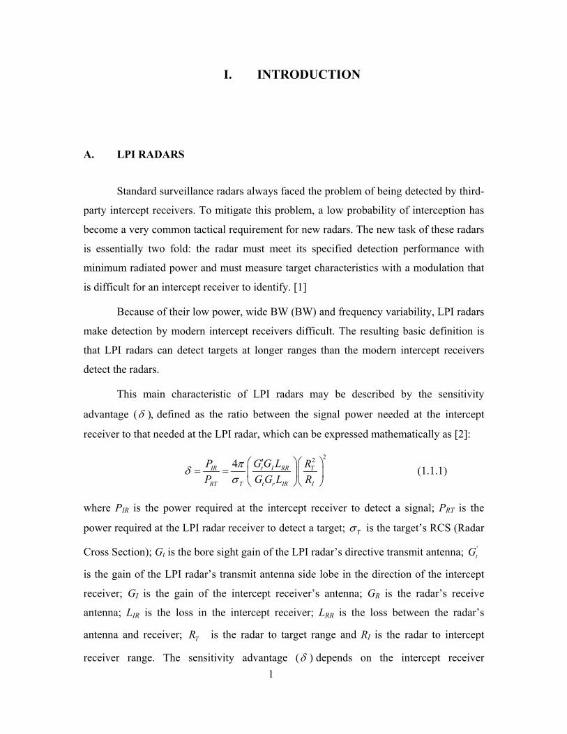
A. LPI RADARS
Standard surveillance radars always faced the problem of being detected by third-
party intercept receivers. To mitigate this problem, a low probability of interception has
become a very common tactical requirement for new radars. The new task of these radars
is essentially two fold: the radar must meet its specified detection performance with
minimum radiated power and must measure target characteristics with a modulation that
is difficult for an intercept receiver to identify. [1]
Because of their low power, wide BW (BW) and frequency variability, LPI radars
make detection by modern intercept receivers difficult. The resulting basic definition is
that LPI radars can detect targets at longer ranges than the modern intercept receivers
detect the radars.
This main characteristic of LPI radars may be described by the sensitivity
advantage (δ ), defined as the ratio between the signal power needed at the intercept
receiver to that needed at the LPI radar, which can be expressed mathematically as [2]:
224 t I RRIR T
RT T t r IR I
G G LP RP G G L R
πδσ
′ = =
(1.1.1)
where PIR is the power required at the intercept receiver to detect a signal; PRT is the
power required at the LPI radar receiver to detect a target; Tσ is the target’s RCS (Radar
Cross Section); Gt is the bore sight gain of the LPI radar’s directive transmit antenna; 'tG
is the gain of the LPI radar’s transmit antenna side lobe in the direction of the intercept
receiver; GI is the gain of the intercept receiver’s antenna; GR is the radar’s receive
antenna; LIR is the loss in the intercept receiver; LRR is the loss between the radar’s
antenna and receiver; TR is the radar to target range and RI is the radar to intercept
receiver range. The sensitivity advantage (δ ) depends on the intercept receiver

2
characteristics and should be a high value, on the order of 50 dB, for a case where we
have a simple receiver against an LPI radar.
The success of LPI radars depends on how hard it is for a receiver to detect the
radars’ emission parameters. The processing capabilities of modern ES (Electronic
Support) equipment are increasing, leading to more specific LPI requirements. On the
receiver side, better results in spectral analysis, for non-cooperative detection and
classification, may be obtained if these radar signals are modeled as cyclostationary.
All digitally modulated signals are cyclostationary, meaning that their
probabilistic parameters vary in time with single or multiple periodicities. One property
that extends from this is that digitally modulated signals have a certain amount of spectral
correlation. In other words, the signal is correlated with frequency-shifted versions of
itself (auto-correlation) at certain frequency shifts. Analyzing LPI radar waveforms using
cyclostationary modeling is advantageous because non-zero correlation is exhibited
between certain frequency components when their separation is related to the periodicity
of interest (e.g., the symbol rate or carrier frequency). The value of that spectral
separation is referred to as the cycle frequency.
Two main algorithms stand out as computationally efficient tools for
cyclostationary signal processing. The first is the time smoothing Fast Fourier Transform
(FFT) Accumulation Method and the other is the Direct Frequency Smoothing Method
[3]. Both tools are implemented in MATLAB® 6.1 for this thesis. [4]
B. PRINCIPAL CONTRIBUTIONS
The objective of the research described in this thesis was to implement in
MATLAB® [4], two computationally efficient cyclostationary algorithms known as the
Time Smoothing FFT Accumulation Method and the Direct Frequency Smoothing
Method, defined in [3] and investigate them as an ES receiver for processing LPI radar
signals.
The first step was to generate the LPI signals in a standardized way. The code
used was called the “LPI Signal Generator,” developed by Fernando Taboada [5], and
also includes contributions by the author of this thesis. The generated modulations were

3
• BPSK (Binary Phase Shift Keying);
• FMCW (Frequency Modulated Continuous Wave);
• Polyphase Codes (P4, P3, P2 P1 and Frank Codes);
• Costas Codes (Frequency Hopping - FH);
• FSK/PSK (Combined Frequency Shift Keying and Phase Shift Keying) with a
Costas frequency distribution; and
• FSK/PSK with a target matched frequency distribution.
Once the signal test matrix was completed, simulations to verify the implementation of
each algorithm were performed in MATLAB® [4] and the results were compared with
other receiver signal processing techniques, such as Higher Order Statistics [5],
Quadrature Mirror Filter Banks [6] and the Wigner Distribution [7].
A Graphic User Interface (GUI) was developed in MATLAB® [4] to simplify the
analysis of the simulation results. The output obtained from the cyclostationary signal
models were then used to determine the various characteristics of each modulation in
question.
Previous work has been done to analyze phase modulation techniques such as
BPSK (Binary Phase-Shift Keying) and QPSK (Quaternary Phase-Shift Keying) using
time-smoothing techniques [8, 9]. In this thesis, both frequency and time-smoothing
techniques are used to analyze various LPI radar modulations and to evaluate the
measurement of the modulation parameters.
C. THESIS OUTLINES
The purpose of this thesis is to document the software implementation of a non-
cooperative cyclostationary receiver for LPI radar waveforms. The remainder of this
thesis supports this purpose and is organized as follows.
Chapter II presents a brief description of Low Probability of Intercept (LPI)
waveforms and their spectral properties. Two FSK and PSK-combined modulations are
discussed and analyzed. BPSK, P4, FMCW and Costas Codes are described in depth in
[5].

4
Chapter III presents the Cyclostationary signal processing algorithms, a brief
description of the cyclostationary processor, the MATLAB® [4] tools and the extracted
parameters description.
Chapter IV shows the analysis of the different modulation types, their parameters,
as well as the simulation results.
Chapter V summarizes the results of this thesis and also makes recommendations
for future research.
Appendix A contains the MATLAB® [4] M-files used for implementation of both
algorithms from [3].
Appendix B contains the MATLAB® [4] M-files for the LPI Generator blocks for
FSK/PSK Costas and Target signals.
Appendix C contains a table of all LPI radar signals analyzed.

5
II. LPI WAVEFORMS DESCRIPTION
A. BACKGROUND
LPI radars are especially designed to oppose external third-party receivers that
attempt to identify the system characteristics and emitter location. Modern electronic
support (ES) receivers can easily detect the high peak power transmitted by pulsed radars.
The use of CW (Continuous Wave) modulations and the ability to manage the transmitted
power limiting emission to the minimum power required to detect typical targets, at the
required range, make LPI radar signals much less detectable. [5] Besides power
management, LPI radars modulate their transmissions spreading the energy in frequency
so that the frequency spectrum of the transmitted signal is wider than required to carry
the signal’s information. Spreading the signal energy reduces the signal-strength-per-
information BW.
LPI waveforms investigated in this thesis include BPSK, FMCW, P4, P3, P2, P1,
Frank Codes, Costas Codes, FSK/PSK with a Costas frequency distribution, and
FSK/PSK with a target matched frequency distribution. Refer to Fernando Taboada’s [5]
thesis work for a detailed description of the other LPI modulations analyzed in this thesis.
The complete matrix of analyzed signals is shown in Appendix C. This thesis presents the
analysis of one signal example per modulation type. The analysis of the rest of the signals
is included in a Technical Report to be published. [10]
This chapter specifically discusses the two modulation types that combine
frequency and phase-shift keying (FSK/PSK combined). One modulation type is a
combination of a Costas frequency-hopping technique and binary phase modulation using
Barker sequences of different lengths. The second is a frequency-hopping technique that
uses the characteristic frequency distribution of a desired target, creating a matched FSK,
which is then modulated with a random-phase keying.
6
B. FSK/PSK COMBINED USING A COSTAS-BASED FREQUENCY-HOPPING (FH) TECHNIQUE
This modulation technique is the result of a combination of frequency-shift
keying based on a Costas frequency-hopping matrix and phase-shift keying using Barker
sequences of different lengths. A thorough description of the implementation of a Costas
frequency-hopping technique is in [5]. The purpose of this section is to describe briefly
the phase encoding applied to a Costas signal, generating the FSK/PSK combined
waveform.
In a Costas frequency-hopped signal, the firing order defines what frequencies
will appear and with what duration. Since we are discussing CW radars, the usual
terminology does not apply to this case. Instead of a “burst” of pulses, we have
frequencies being continuously emitted during a defined period of time. This period may
be divided into sub-periods, labeled TF for each frequency. The length of each sub-period
depends on the sampling interval. During each sub-period, the signal frequency (one of
the FN frequencies) is modulated by a binary phase sequence according to a Barker
sequence of length five (+ + + - +), seven (+ + + - - + -), eleven (+ + + - - - + - - + -) or
thirteen (+ + + + + - - + + - + - +). For example, the FSK/PSK signal defined by S = 1+,
1+, 1+, 1-, 1+, 2+, 2+, 2+, 2-, 2+, 3+, 3+, 3+, 3-, 3+, 4+, 4+, 4+, 4-, 4+, 5+, 5+, 5+, 5-, 5+,
represents a waveform comprised of 5FN = different frequencies, that are each
subdivided into five phase slots, labeled TP, according to the Barker sequence of length
five (+ + + - +). The final waveform may be seen as a binary phase-shifting modulation
within each frequency hop, resulting in 5 phase slots equally distributed in each
frequency slot, giving a total of 25 phase slots.
As illustrated in Figure 1, if we consider FN as the number of frequency hops and
PN as the number of phase slots of duration TP (Chip Period) in each frequency sub-
period TF, the total number of phase slots in the FSK/PSK waveform is given by:
* F PN N N= (2.1.1)
7
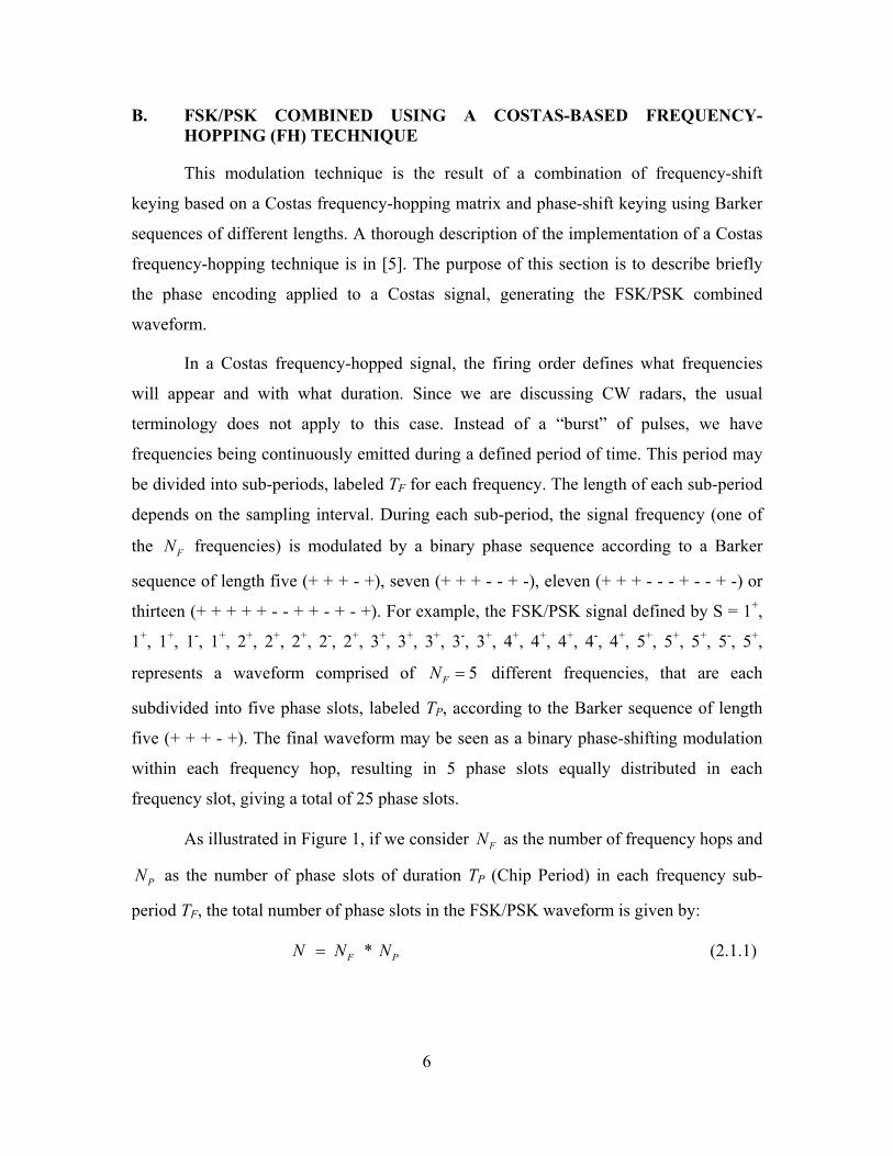
The block diagram in Figure 1 describes the MATLAB® [4] implementation. The
user defines which sequence of Costas frequency hops to be used and also how long the
Barker sequence is (5, 7, 11 or 13). The number of frequency hops is pre-defined to be
“seven” and the user may select from two different frequency sequences, varying from
1kHz to 8kHz. The Costas matrix used in the implementation is the following:
Costas Sequence 1 4 7 1 6 5 2 3
Costas Sequence 2 2 6 3 8 7 5 1 Frequencies (kHz)
• → • → .
Figure 1 a) FSK/PSK Costas LPI Generator MATLAB® [4] code block
diagram and, b) general FSK/PSK signal containing NF frequency hops with NP phase slots per frequency.
The Barker sequence is generated and the frequency-hopping signal is then phase-
modulated accordingly. For example, if the first Costas sequence is selected, after a phase
modulation using a Barker sequence of length 5, the final waveform becomes S = 4+, 4+,
8
4+, 4-, 4+, 7+, 7+, 7+, 7-, 7+, 1+, 1+, 1+, 1-, 1+, 6+, 6+, 6+, 6-, 6+, 5+, 5+, 5+, 5-, 5+, 2+, 2+, 2+, 2-,
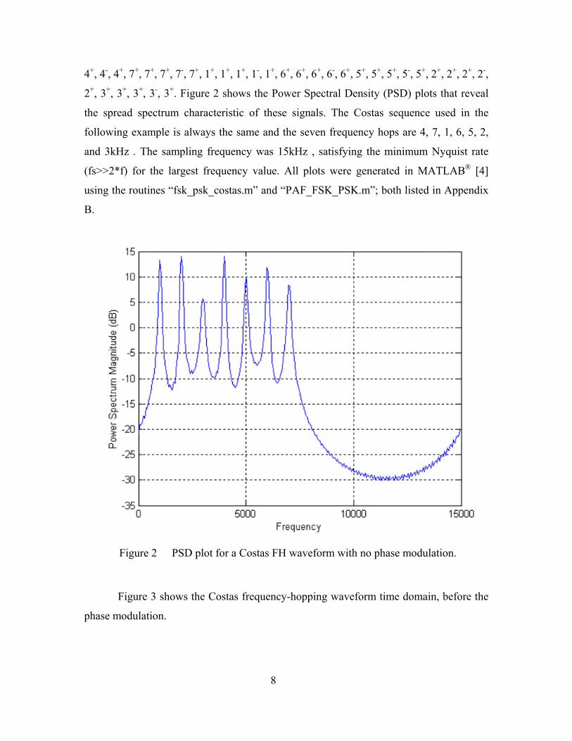
2+, 3+, 3+, 3+, 3-, 3+. Figure 2 shows the Power Spectral Density (PSD) plots that reveal
the spread spectrum characteristic of these signals. The Costas sequence used in the
following example is always the same and the seven frequency hops are 4, 7, 1, 6, 5, 2,
and 3kHz . The sampling frequency was 15kHz , satisfying the minimum Nyquist rate
(fs>>2*f) for the largest frequency value. All plots were generated in MATLAB® [4]
using the routines “fsk_psk_costas.m” and “PAF_FSK_PSK.m”; both listed in Appendix
B.
Figure 2 PSD plot for a Costas FH waveform with no phase modulation.
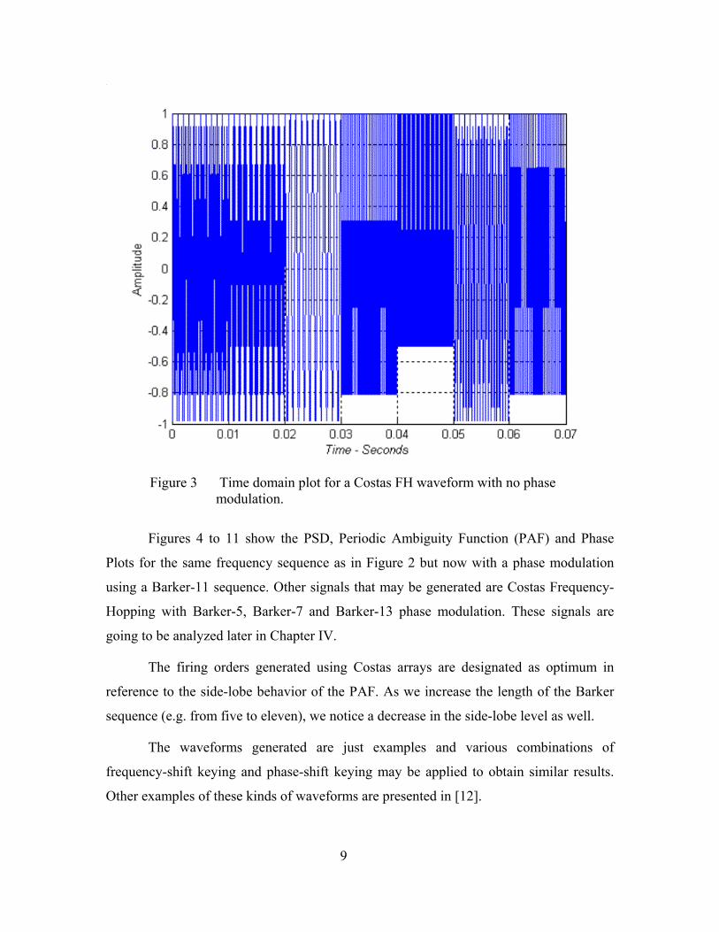
Figure 3 shows the Costas frequency-hopping waveform time domain, before the
phase modulation.
9
Figure 3 Time domain plot for a Costas FH waveform with no phase
modulation.
Figures 4 to 11 show the PSD, Periodic Ambiguity Function (PAF) and Phase
Plots for the same frequency sequence as in Figure 2 but now with a phase modulation
using a Barker-11 sequence. Other signals that may be generated are Costas Frequency-
Hopping with Barker-5, Barker-7 and Barker-13 phase modulation. These signals are
going to be analyzed later in Chapter IV.
The firing orders generated using Costas arrays are designated as optimum in
reference to the side-lobe behavior of the PAF. As we increase the length of the Barker
sequence (e.g. from five to eleven), we notice a decrease in the side-lobe level as well.
The waveforms generated are just examples and various combinations of
frequency-shift keying and phase-shift keying may be applied to obtain similar results.
Other examples of these kinds of waveforms are presented in [12].
10
The PAF plots were performed both for a complete period for all Costas
frequencies in the sequence and for only one period in one frequency hop. Therefore, the
Costas PAF characteristics as well as the BPSK PAF characteristics may be compared.
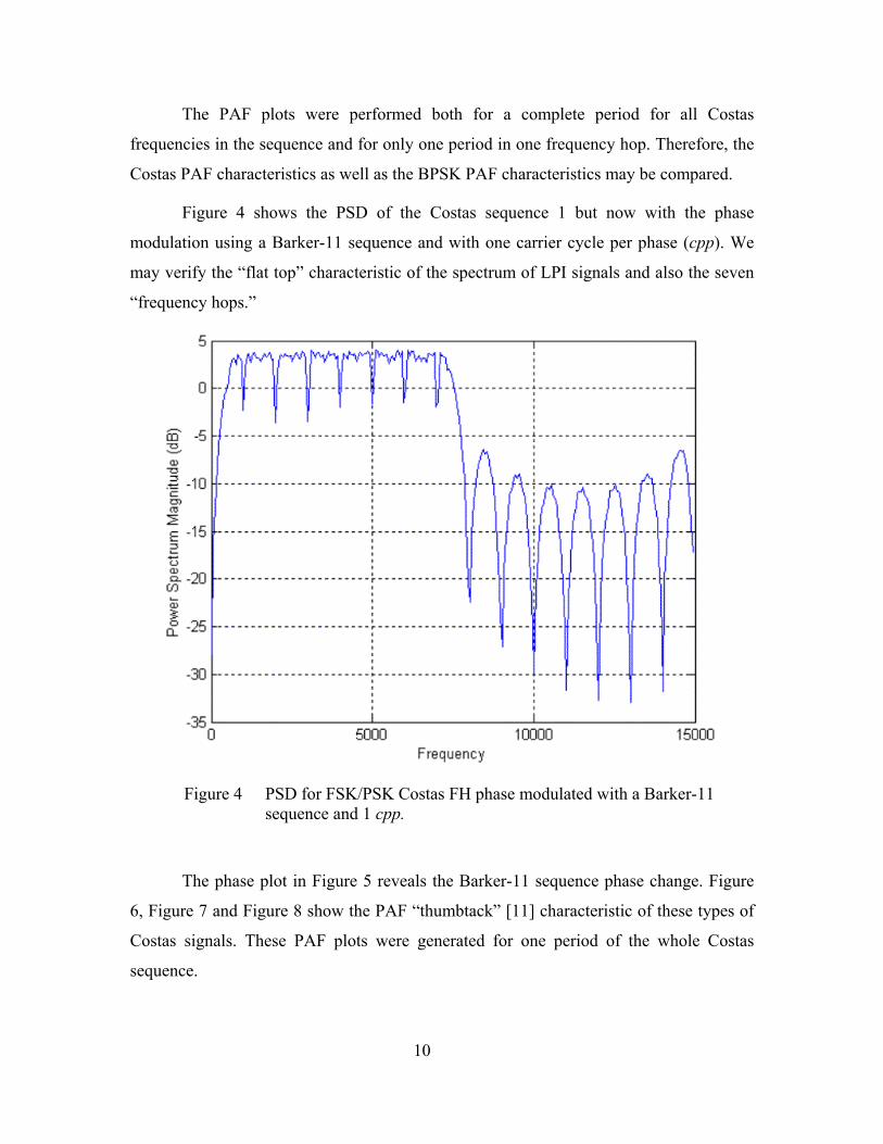
Figure 4 shows the PSD of the Costas sequence 1 but now with the phase
modulation using a Barker-11 sequence and with one carrier cycle per phase (cpp). We
may verify the “flat top” characteristic of the spectrum of LPI signals and also the seven
“frequency hops.”
Figure 4 PSD for FSK/PSK Costas FH phase modulated with a Barker-11
sequence and 1 cpp.
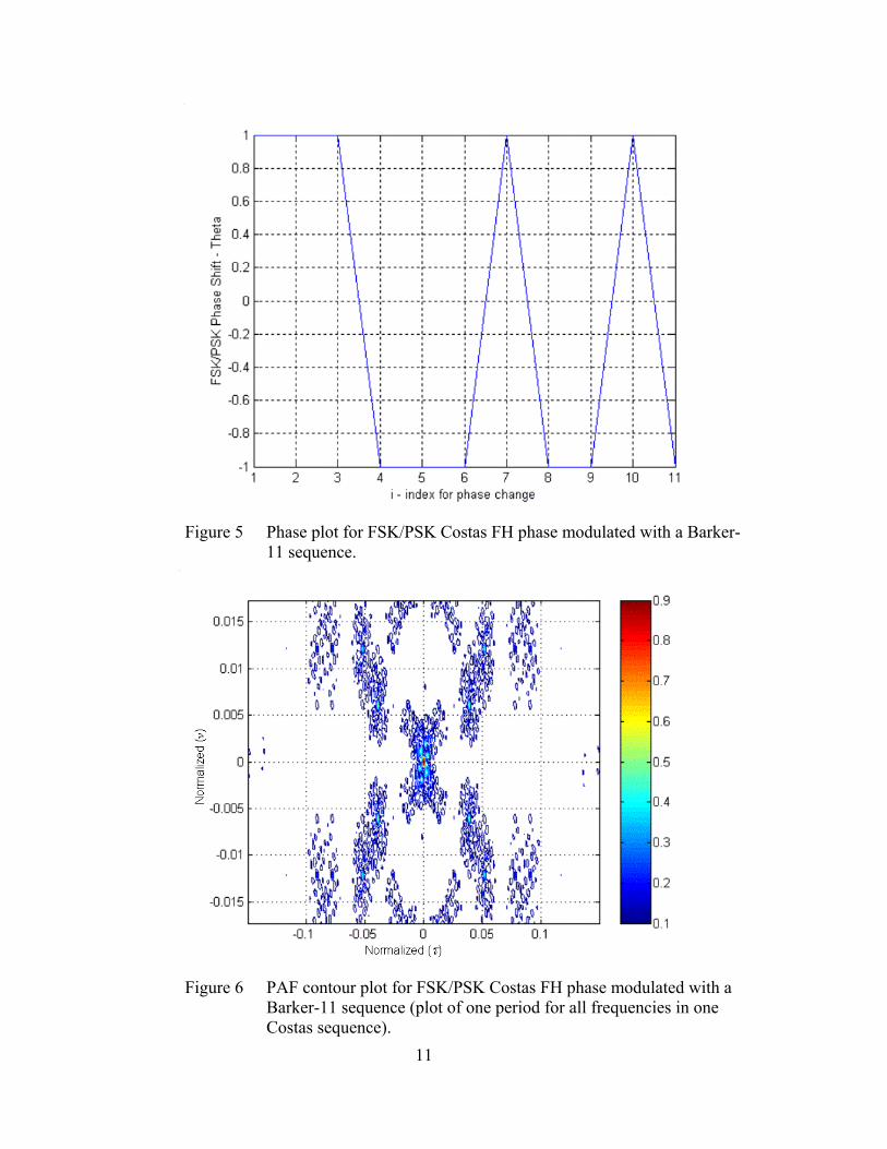
The phase plot in Figure 5 reveals the Barker-11 sequence phase change. Figure
6, Figure 7 and Figure 8 show the PAF “thumbtack” [11] characteristic of these types of
Costas signals. These PAF plots were generated for one period of the whole Costas
sequence.
11
Figure 5 Phase plot for FSK/PSK Costas FH phase modulated with a Barker-
11 sequence.
Figure 6 PAF contour plot for FSK/PSK Costas FH phase modulated with a
Barker-11 sequence (plot of one period for all frequencies in one Costas sequence).

12
Figure 7 PAF delay axis cut for FSK/PSK Costas FH phase modulated with a
Barker-11 sequence (plot of one period for all frequencies in one Costas sequence).
Figure 8 PAF Doppler axis cut for FSK/PSK Costas FH phase modulated with
a Barker-11 sequence (plot of one period for all frequencies in one Costas sequence).

13
Figure 9, Figure 10 and Figure 11 show the modulation for one period of one
frequency hop of the Costas sequence used in Figure 2. Each frequency hop has similar
PAF characteristics of a single carrier frequency BPSK signal. The plots of these Figures
were done for the first carrier frequency of the first Costas sequence. Other modulation
examples are analyzed later in Chapter IV.
Figure 9 PAF contour plot for FSK/PSK Costas FH phase modulated with a
Barker-11 sequence (plot of one period for one frequency in the Costas sequence).

14
Figure 10 PAF delay axis cut for FSK/PSK Costas FH phase modulated with a
Barker-11 sequence (plot of one period for one frequency in the Costas sequence).
Figure 11 PAF Doppler axis cut for FSK/PSK Costas FH phase modulated with
a Barker-11 sequence (plot of one period for one frequency in the Costas sequence).
15
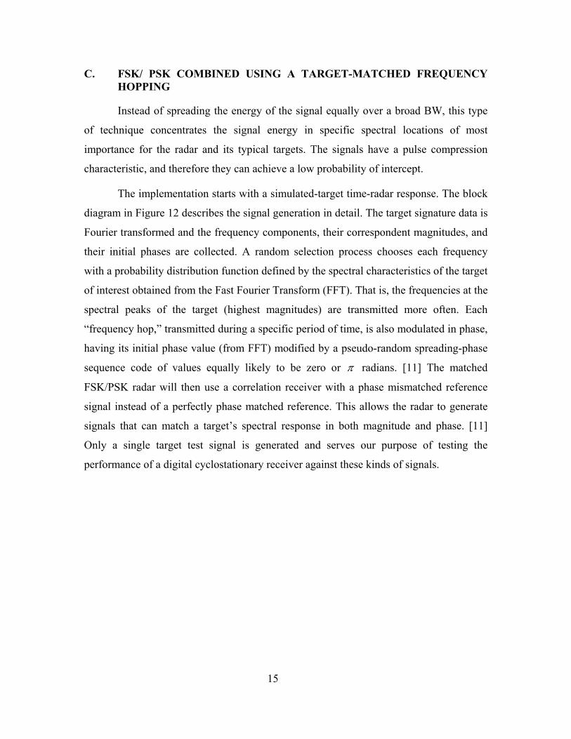
C. FSK/ PSK COMBINED USING A TARGET-MATCHED FREQUENCY HOPPING
Instead of spreading the energy of the signal equally over a broad BW, this type
of technique concentrates the signal energy in specific spectral locations of most
importance for the radar and its typical targets. The signals have a pulse compression
characteristic, and therefore they can achieve a low probability of intercept.
The implementation starts with a simulated-target time-radar response. The block
diagram in Figure 12 describes the signal generation in detail. The target signature data is
Fourier transformed and the frequency components, their correspondent magnitudes, and
their initial phases are collected. A random selection process chooses each frequency
with a probability distribution function defined by the spectral characteristics of the target
of interest obtained from the Fast Fourier Transform (FFT). That is, the frequencies at the
spectral peaks of the target (highest magnitudes) are transmitted more often. Each
“frequency hop,” transmitted during a specific period of time, is also modulated in phase,
having its initial phase value (from FFT) modified by a pseudo-random spreading-phase
sequence code of values equally likely to be zero or π radians. [11] The matched
FSK/PSK radar will then use a correlation receiver with a phase mismatched reference
signal instead of a perfectly phase matched reference. This allows the radar to generate
signals that can match a target’s spectral response in both magnitude and phase. [11]
Only a single target test signal is generated and serves our purpose of testing the
performance of a digital cyclostationary receiver against these kinds of signals.

16
Figure 12 Block diagram of the MATLAB® [4] implementation of FSK/PSK
target matched waveform.
Figure 13 shows the 64 complex points target range radar response plot. Figure 14
reveals the 64 frequency components that will be selected randomly 256 times. Figure 15
illustrates the frequency firing order, Figure 16 illustrates the PSD and Figures 17, 18 and
19 illustrate the PAF properties of these signals. Figure 15 shows the histogram of the 64
frequency components and shows the number of occurrences of each frequency. Note
that this is similar to the FFT output or probability distribution shown in Figure 14. The
following figures show one signal example with 5 carrier periods per phase and 256
frequency hops. Figure 16 shows the PSD plots and reveals the highly spread-spectrum
characteristics of this type of modulation. Note the noise-like behavior due to the random
phase modulation.

17
Figure 13 FSK/PSK target 64 complex points radar range simulated response.
Figure 14 FSK/PSK target frequency probability distribution of 64 frequency
components.

18
Figure 15 FSK/PSK target 64 frequency components histogram with number of
occurrences per frequency for 256 frequency hops.
Figure 16 PSD for FSK/PSK target with 64 frequency components, 256
frequency hops, random phase modulation and 5 cpp.

19
Figure 17 PAF contour plot for FSK/PSK target with 64 frequency components,
256 frequency hops, random phase modulation and 5 cpp.
Figure 18 PAF delay cut for FSK/PSK target with 64 frequency components,
256 frequency hops, random phase modulation and 5 cpp.

20
Figure 19 PAF Doppler cut for FSK/PSK target with 64 frequency components,
256 frequency hops, random phase modulation and 5 cpp.
An extensive discussion regarding the PAF “thumbtack” characteristic of these types of
waveforms, as shown in the last three Figures, are presented in Donohoe et al in [11].
In this chapter we discussed the implementation of two complex LPI Radar
signals using FSK and PSK techniques combined. A brief theoretical and practical
tutorial on cyclostationarity processing and its implementation using the FFT
Accumulation Method and the Direct Frequency Smoothing Method is given in the next
chapter.

21
III. CYCLOSTATIONARY SIGNAL PROCESSING ALGORITHMS AND TUTORIAL
This chapter briefly explains the cyclostationary processes, the time-smoothing
(FAM) and frequency-smoothing (DFSM) algorithms and how they were implemented.
A thorough description on cyclostationarity and its properties may be found in [12], [13]
and [14].
A. CYCLOSTATIONARY THEORY
The cyclostationary theory for signal processing, as described by William A.
Gardner [12], involves three main properties:
• Generation of spectral lines by quadratically transforming a signal;
• The statistical property called “second-order cyclostationarity,” namely the
periodic fluctuation of the auto-correlation function with time;
• The correlation property for signal components in distinct spectral bands.
The cyclostationary attribute, as it is reflected in the periodicities of the second
order moments of the signal, can be interpreted in terms of the generation of spectral lines
from the signal by putting the signal through a quadratic non-linear transformation. This
property explains the link between the spectral-line generation property and the statistical
property called “spectral correlation”, corresponding to the correlation that exists
between the random fluctuations of components of the signal residing in distinct spectral
bands. The correlation integral is very important in theoretical and practical applications
and may be defined as
( ) ( ) ( )h x f u g x u du∞
−∞
= +∫ (3.1.1)
Applying an FFT, it forms a Fourier transform pair given by:
{ }( ) ( ) *( )ℑ =h x F s G s (3.1.2)
22
If f(x) and g(x) are the same function, the integral above is normally called the
autocorrelation function and called cross-correlation if they differ. The autocorrelation
function is a quadratic transformation of a signal and may be interpreted as a measure of
the predictability of the signal at time t +τ based on knowledge of the signal at time t.
[13]
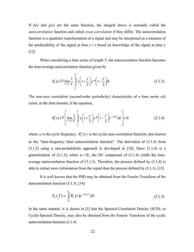
When considering a time series of length T, the autocorrelation function becomes
the time-average autocorrelation function given by
2
2
1( ) lim *2 2τ ττ
→∞−
+ − ∫
T
x TT
R x t x t dtT
(3.1.3)
The non-zero correlation (second-order periodicity) characteristic of a time series x(t)
exists, in the time domain, if the equation,
22
2
1( ) lim * 02 2
T
j tx T
T
R x t x t e dtT
α πατ ττ −
→∞−
+ − ≠
∫ (3.1.4)
where α is the cycle frequency. ( )xRα τ is the cyclic auto-correlation function, also known
as the “time-frequency limit autocorrelation function”. The derivation of (3.1.4) from
(3.1.3) using a non-probabilistic approach is developed in [10]. Since (3.1.4) is a
generalization of (3.1.3), when α = 0 , the DC component of (3.1.4) yields the time-
average autocorrelation function of (3.1.3). Therefore, the process defined by (3.1.4) is
able to extract more information from the signal than the process defined by (3.1.3). [13]
It is well known that the PSD may be obtained from the Fourier Transform of the
autocorrelation function (3.1.3). [14]
2( ) ( ) π ττ τ∞
−
−∞
= ∫ i fx xS f R e d (3.1.5)
In the same manner, it is shown in [3] that the Spectral-Correlation Density (SCD), or
Cyclic-Spectral Density, may also be obtained from the Fourier Transform of the cyclic
autocorrelation function (3.1.4)

23
2 *1( ) ( ) lim2 2
α α π τ α ατ τ∞
−
→∞−∞
= + − ∫ i f
x x T TTS f R e d X f X f
T (3.1.6)
where α is the cycle frequency and:
22
2
( ) ( ) π−
−∫T
j fuT
T
X f x u e du (3.1.7)
which is the Fourier Transform of the time domain signal x(u). The additional variable
α leads to a two-dimensional representation ( )αxS f , in the bi-frequency plane or (f, α )
plane. [12]
The spectral correlation exhibited by cyclostationary or almost cyclostationary
processes is completely characterized by the cyclic spectra ( αxS ) or characterized
equivalently by the cyclic autocorrelations ( αxR ). [12] In practice, the cyclic-spectral
density must be estimated because the signals being considered are defined over a finite
time interval ( ∆ t), and therefore the cyclic-spectral density cannot be measured exactly.
Estimates of the cyclic-spectral density can be obtained via time or frequency-smoothing
techniques. In this work we will be able to compare both methods when analyzing LPI
radar signals.
An estimate of the SCD can be obtained by the time-smoothed cyclic
periodogram is given by [10]:
2
2
1( ) ( , ) ( , )α α
∆+
∆∆
−
≈ =∆ ∫T TW W
tt
x x t xtt
S f S t f S u f dut (3.1.8)
where
*1( , ) , ,2 2α α = + −
T W WWx T TW
S u f X u f X u fT (3.1.9)
and ∆ t = total observation time of the signal, TW = short-time FFT window length, and:

24
( )2
2
2
, ( )
W
W
W
Tt
j fuT
Tt
X u f x u e duπ
+
−
−
= ∫ (3.1.10)
is the sliding short-time Fourier Transform, and is a viable solution for computing the
SCD estimations. Using a graphical explanation, in Figure 20, for some signal x(t) the
frequency components are evaluated over a small time window TW (sliding FFT time
length), along the entire observation time interval ∆t. [12] The spectral components
generated by each short-time Fourier Transform have a resolution, 1W
f T∆ = . In Figure
20, L is the overlapping factor between each short-time FFT. In order to avoid aliasing
and cycle leakage on the estimates, the value of L is defined as 4WTL ≤ . [12]
Figure 20 Pictorial illustration of the estimation of the time-variant spectral
periodogram (adapted from [12, 17]).

25
Figure 21 shows that the spectral components of each short-time FFT are
multiplied, still providing the same resolution capability 1W
f T∆ = , for the cyclic-
spectrum estimates. Note that the dummy variable u has been replaced by the time
instances 1... pt t . At each window (TW), two components centered about some f0 and
separated by some 0α are multiplied together and the resulting sequence of products is
then integrated over the total time ( t∆ ), as shown in (3.1.8).
Figure 21 Sequence of frequency products for each short-time Fourier
transforms (adapted from [12, 17]).
The estimation ( ) ( , )α α∆≈
TWx x tS f S t f can be made as reliable and accurate as
desired for any given t and ∆f, and for all f by making ∆t sufficiently large, provided that
equation (3.1.4) exists within the interval ∆t and that a substantial amount of smoothing
is carried out over ∆t, which leads to the Grenander’s Uncertainty Condition * 1t f∆ ∆
[12]. This Uncertainty Condition means that the observation time ( t∆ ) must greatly

26
exceed the time window (TW), which is used to compute the spectral components. A data
taper window is also used to minimize the effects of cycle and spectral leakage
(estimation noise), introduced by frequency component side-lobes. [12]
If we consider the fact that the cycle frequency estimate is 1 tα∆ ≈ ∆ , it results
that the estimation of some (f0, 0α ) represents a very small area on the bi-frequency plane
as shown in Figure 22 and since one needs a significant number of estimates to represent
the cyclic spectrum adequately, it follows that obtaining estimates may become very
computationally demanding. [12]
Figure 22 Bi-frequency plane, frequency and cycle frequency resolutions on
detailed area (adapted from [12, 17]).

27
B. DISCRETE TIME CYCLOSTATIONARY ALGORITHMS
The computationally efficient algorithms for implementation of time and
frequency-smoothing techniques are discussed in [3]. These are the FFT Accumulation
Method (FAM) and the Direct Frequency-Smoothing Method (DFSM) as described
below. The temporal and spectral smoothing equivalence is also addressed in [12]. The
computationally efficient algorithms for implementation of time and frequency-
smoothing techniques are extensively discussed in [3].
1. The Time-Smoothing FFT Accumulation Method (FAM):
The time-smoothing FFT Accumulation Method was developed to reduce the
number of computations required to estimate the cyclic spectrum. [3] This technique
divides the bi-frequency plane into smaller areas called the channel-pair regions and
computes the estimates a block at a time using the Fast Fourier Transform. Describing the
estimated time-smoothed periodogram from Equations (3.1.8) and (3.1.9), in discrete
terms, yields
' '
1*
'0
1 1( , ) , ,' 2 2
γ γ γ−
=
= + − ∑N N
N
x N Nn
S n k X n k X n kN N (3.2.1)
where
[ ] [ ]2' 1
''
0
( , )π−−
=∑
j knNN
Nn
X n k w n x n e , (3.2.2)
is the Discrete Fourier Transform of x[n], w[n] is the data taper window (e.g. Hamming
window) and the discrete equivalents of f and α are k and γ respectively. Figure 23
represents a block diagram [13] used in the implementation of this method in
MATLAB®. [4]

28
Figure 23 FAM block diagram (adapted from [3, 13]).
The algorithm consists of three basic stages: computation of the complex
demodulates (divided into data tapering, sliding 'N point Fourier transforming and base
band frequency-downshift translation sections), then computation of the product
sequences and smoothing of the product sequences. Making a parallel between the
variables in equations (3.1.8), (3.1.9) and (3.2.1), we have:
NAME CONTINOUS TIME DISCRETE TIME
SCD ( , )TWx tS t fα
∆ '( , )
Nx NS n kγ
Short FFT Size TW 'N
Observation Time t∆ N
Time t n
Frequency f k
Cycle Frequency α γ
Grenander’s Uncertainty
Condition 1fM α
∆= ∆ 1'NM N=
Table 1. Comparison of the estimated time-smoothed Periodogram expressed in continuous and discrete time.

29
The parameter N represents the total number of discrete instances within the oservatio
time and 'N represents the number of pints within the discrete short-time sliding FFT. In
the FAM algorithm, spectral components of a sequence, x[n], are computed using (3.2.2).
Two components are multiplied (3.2.1) to provide a sample of a cyclic spectrum estimate
representing a finite area on the bi-frequency plane called a “channel pair region,” as
shown in Figure 24. There are 2N channel pair regions in the bi-frequency plane. Note
the sixteen small channel pair regions corresponding to a value of N = 4 in Figure 24.
Figure 24 Division of bi-frequency plane in channel pair regions (adapted from
[3, 15]).
A sequence of samples for any particular area may be obtained by multiplying the same
two components of a series of consecutive short-time sliding FFT's along the entire
length of the input sequence. After the channelization performed by an 'N -point FFT
sliding over the data with an overlap of L samples, the outputs of the FFT’s were shifted
in frequency in order to obtain the complex demodulate sequences (see Figure 23). [3]

30
Instead of computing an average of the product of sequences between the complex
demodulates, as in (3.1.8), they are Fourier transformed with a P-point (second) FFT. The
computational efficiency of the algorithm is improved by a factor of L since only NL
samples are processed for each point estimate. With Sf the sampling frequency, the cycle
frequency resolution of the decimated algorithm is defined as Sres
fNγ = (compare to
1tα∆ = ∆ ), the frequency resolution is '
Sres
fk N= (compare to 1W
f T∆ = ) and the
Grenander’s Uncertainty Condition is 1'N
N (compare to 1t f∆ ⋅∆ ). Figure 25,
clearly reveals that the estimates toward the top and the bottom (yellow areas) of the
channel pair region do not satisfy the Uncertainty Condition.
Figure 25 Cycle frequency and frequency resolutions and the Grenander’s
Uncertainty Condition (adapted from [3, 13]).
In order to minimize the variability of these point estimates, we can retain only
those cyclic spectrum components that are within of 2reskγ = ± from the center of the

31
channel pair region. [15] A solution to resolve the entire area of the channel pair region
without leaving gaps is to apply a data taper window on the frequency axis to obtain
better coverage. A Hamming window is applied in this implementation.
2. Direct Frequency-Smoothing Method:
Direct frequency-smoothing algorithms first compute the data frequency
components and then execute spectral-correlation operations directly on the frequency
components. Generally, the Direct Frequency-Smoothing Method (DFSM) is
computationally superior to indirect algorithms that use related quantities, such as the
Wigner-Ville Distribution. [12] But DFSM is normally less efficient than a time-
smoothing approach.
Time and frequency-smoothing equivalence is discussed in details in [10] and
derives from the fact that randomly fluctuating statistical spectra (in both time and
frequency), such as ( )1
,f
x tS t fα
∆∆
(compare to 3.1.8, where 1WT f= ∆ ) and ( , )
x t fS t fα
∆∆ ,
converge in the limit ( ), 0∆ → ∞ ∆ →t f to the non-random limit spectrum ( )xS fα if the
limit autocorrelation ( )xRα τ exists. Employing discrete frequency averaging and
following the same analogy as in the time-smoothed cyclic periodogram, the basis for the
DFSM is the discrete time frequency-smoothed cyclic periodogram represented by
*( , ) , ,2 2N Nx k N
mS n k X n k X n kγ γ γ
∆ = + −
∑ (3.3.1)
where
[ ] [ ]21
0
( , )j knNN
Nn
X n k w n x n eπ−−
=∑ , (3.3.2)
is the Discrete Fourier Transform of x[n], w[n] is a rectangular window of length N that is
the total number of points of the FFT related to the total observation time ∆t , γ is the
cycle frequency discrete equivalent, the frequency-smoothing ranges over the interval
2≤ Mm and ⋅∆ ≈ SM fk N is the frequency resolution discrete equivalent.[12] All

32
considerations made previously in Section A (Cyclostationary Theory) are still valid and,
for 1M , the frequency and time smoothing methods will yield very similar results.
The block diagram on Figure 26 [13] illustrates the implementation of the “DFSM.m”
MATLAB® [4] routine.
Figure 26 DFSM algorithm block diagram (adapted from [3, 13]).
In order to provide full coverage of the bi-frequency plane at a minimal
computational expense, Equation (3.3.1) is computed along a line of constant cycle
frequency spacing the point estimates by SM fk N⋅∆ = . This method is easier to
implement and generally is used to validate the time-smoothing “FAM.m” code, but this
method may become more computationally demanding, mainly in the last block in which
the complex-demodulates product sequences are summed. Considerations on the parallel
processing of both time and frequency algorithms are discussed in [13]. Combinations of
both methods are also advantageous for certain applications.
Tthe FAM routine took considerably less time than the DFSM routine. The
computing time for the DFSM was two or three times longer than the FAM for signals
with a large number of samples. Therefore, for very long signals and large M t f= ∆ ∆ ,
FAM should be used to calculate the complete cyclic spectrum.

33
3. GUI Implementation:
A Graphical User Interface (GUI), as shown in Figure 27, was developed using
the MATLAB® GUIDE Version 6 [4] in order to facilitate the execution of the
mathematical model processing.
Figure 27 Cyclostationary processing GUI schematic tutorial.
In this GUI, generated by the MATLAB® [4] routines “cyclo.m”, “FAM.m” and
“DFSM.m”, the user defines
• The directory where the data file is to be located;
• The name of the file (without the extension);
• The sampling frequency;
• The desired frequency resolution ( resk ); and
• The Grenander’s Uncertainty Condition 'NM N= may be chosen to be
equal to 2 or 4.
These variables are then used to calculate
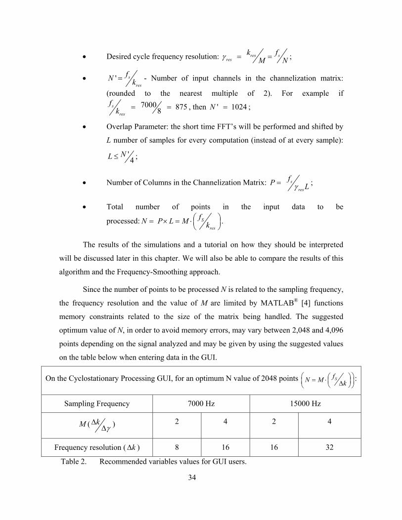
34
• Desired cycle frequency resolution: res sres
k fM Nγ = = ;
• ' s
res
fN k= - Number of input channels in the channelization matrix:
(rounded to the nearest multiple of 2). For example if 7000 8758
s
res
fk = = , then ' 1024N = ;
• Overlap Parameter: the short time FFT’s will be performed and shifted by
L number of samples for every computation (instead of at every sample):
'4
NL ≤ ;
• Number of Columns in the Channelization Matrix: s
res
fP Lγ= ;
• Total number of points in the input data to be
processed: S
res
fN P L M k = × = ⋅
.
The results of the simulations and a tutorial on how they should be interpreted
will be discussed later in this chapter. We will also be able to compare the results of this
algorithm and the Frequency-Smoothing approach.
Since the number of points to be processed N is related to the sampling frequency,
the frequency resolution and the value of M are limited by MATLAB® [4] functions
memory constraints related to the size of the matrix being handled. The suggested
optimum value of N, in order to avoid memory errors, may vary between 2,048 and 4,096
points depending on the signal analyzed and may be given by using the suggested values
on the table below when entering data in the GUI.
On the Cyclostationary Processing GUI, for an optimum N value of 2048 points SfN M k = ⋅ ∆
:
Sampling Frequency 7000 Hz 15000 Hz
M ( kγ
∆∆ ) 2 4 2 4
Frequency resolution ( k∆ ) 8 16 16 32
Table 2. Recommended variables values for GUI users.

35
The platform for all the simulations was a Pentium IV, 2 GHz CPU clock and
1GB RAM. The most critical memory constraints appeared while using the “contour.m”
MATLAB® [4] built-in function, but since this is the plot with the best visualization, we
decided to keep an average maximum number of points of 2,048 whenever possible.
Moreover, by increasing the value of N from 2048 to 4096 or more only improved
the results a little. And since the data files were standardized for comparison with the
results from the methods described in [5], [6] and [7], the input signals were generated to
have characteristics that would facilitate measuring for all four processing types
simultaneously.
All the files in the Cyclostationary MATLAB® [4] package (“cyclo.m, FAM.m
and dfsm.m”) can be edited very easily to include new capabilities. The function
“cyclo.m” triggers the GUI and after entering the data, the user may choose between time
or frequency-smoothing method by clicking the appropriate button. Additional features
and options to the GUI (“Cyclo.fig”) may be added by using the MATLAB® GUIDE [4]
and by editing “cyclo.m” accordingly.
C. PROCESSING TUTORIAL
In order to give a general idea of how the results of both processing methods
should look, this section provides some examples of the signals analyzed.
1. Test Signals:
For this example, the input complex signals characteristics are as following:
Carrier Frequency (fc) 1000 Hz
Sampling Frequency (fs) 7000 Hz Table 3. Test signal characteristics.
This signal is composed of a single carrier sampled at fs=1000Hz; using the real
part of the signal we expect that the plot on the bi-frequency plane will have the carrier
frequency at twice its value, as shown in Figure 28 (DFSM SCD for a Test Signal with N
= 1024, df = 16 and M = 2).
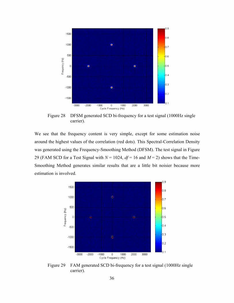
36
Figure 28 DFSM generated SCD bi-frequency for a test signal (1000Hz single
carrier).
We see that the frequency content is very simple, except for some estimation noise
around the highest values of the correlation (red dots). This Spectral-Correlation Density
was generated using the Frequency-Smoothing Method (DFSM). The test signal in Figure
29 (FAM SCD for a Test Signal with N = 1024, df = 16 and M = 2) shows that the Time-
Smoothing Method generates similar results that are a little bit noisier because more
estimation is involved.
Figure 29 FAM generated SCD bi-frequency for a test signal (1000Hz single
carrier).

37
2. BPSK:
For the BPSK (Barker Code) example, the signals characteristics are as following:
Carrier Frequency (fc) 1000Hz.
Sampling Frequency (fs) 7000Hz.
Barker Code Length (Np) 11 bits
SNR Only signal
Number of Carrier Cycles per Barker Bit (NPBB) 1 Table 4. BPSK signal characteristics.
In Figure 30, “k” is the frequency, “γ ” is the cycle frequency, “fC” is the carrier,
“fs” is the sampling frequency, “fb” is the code rate ( )1
bf TpNp =
, “Np” is the number
of phase changes, related to the length of the Barker sequence used in the phase
modulation, and “Tp” is the chip period.
Figure 30 Pictorial generic illustration of a BPSK signal SCD result.

38
By zooming in on the plot, as shown in Figure 31 and in the examples on Figure
32 and Figure 33, we can measure the code rate “fb”, in the cycle frequency axis. It is
possible to see a pattern of equally spaced points that will eventually fade away as the
magnitude decreases (from red to blue). By changing the background color of the contour
plots in order to facilitate establishing a visual threshold (around 0.4 on the normalized
values, or “light blue” on the color bar) to eliminate the estimation errors, we can
approximately determine the BW of the signal being analyzed and this value will then
divided by the code rate “fb”, giving the value of “Np” ( bbandwidth Np f= × ).
Figure 31 Zoomed in pictorial generic illustration of a BPSK signal SCD result
with estimation of BW, number of phases and code rate.

39
Figure 32 DFSM generated SCD plot for a BPSK signal (1000Hz single carrier
and 11 bits Barker-code phase modulation) with estimated BW.
Figure 33 Zoomed-in DFSM generated SCD plot for a BPSK signal (estimated
code rate measurement).

40
The estimation of the BW using this method is somewhat subjective and may lead
to still acceptable errors on the order of bf± . From the plots above we may consider the
values:
• Carrier frequency (fC) = 1000 Hz (directly from plot);
• Code rate, from zoomed-in plots, ( )1 90 bf HzTpNp
= ≅
;
• BW (directly from plot) 1000 90Hz Hz≈ ± ;
• Number of Barker Bits ( Np ) ≈ 1000 11.11 11 bits90= = ≈b
BWf .
This procedure of zooming-in the plots and measuring the distances between the
highest magnitudes (red) points will be used for all the signals analyzed in the next
chapter.
3. FMCW:
For the FMCW case, the signal characteristics are as following:
Carrier Frequency (fC) 1000 Hz.
Sampling Frequency (fS) 7000 Hz.
Modulation Band Width ( ∆ F) 250 Hz
SNR Only signal
Modulation Period (tm) 20 ms Table 5. FMCW signal characteristics.
The same behavior showed by BPSK appears here. Figure 34 and Figure 35 show
that the carrier frequency appears at twice its value on the cycle-frequency axis and that
the Modulation BW and the modulation period may also be estimated by measuring the
distance from the center of the SCD result to the edge, on the k = 0 axis and by measuring
the distance (“delta”) between two consecutive high correlation points in the cycle
frequency axis.
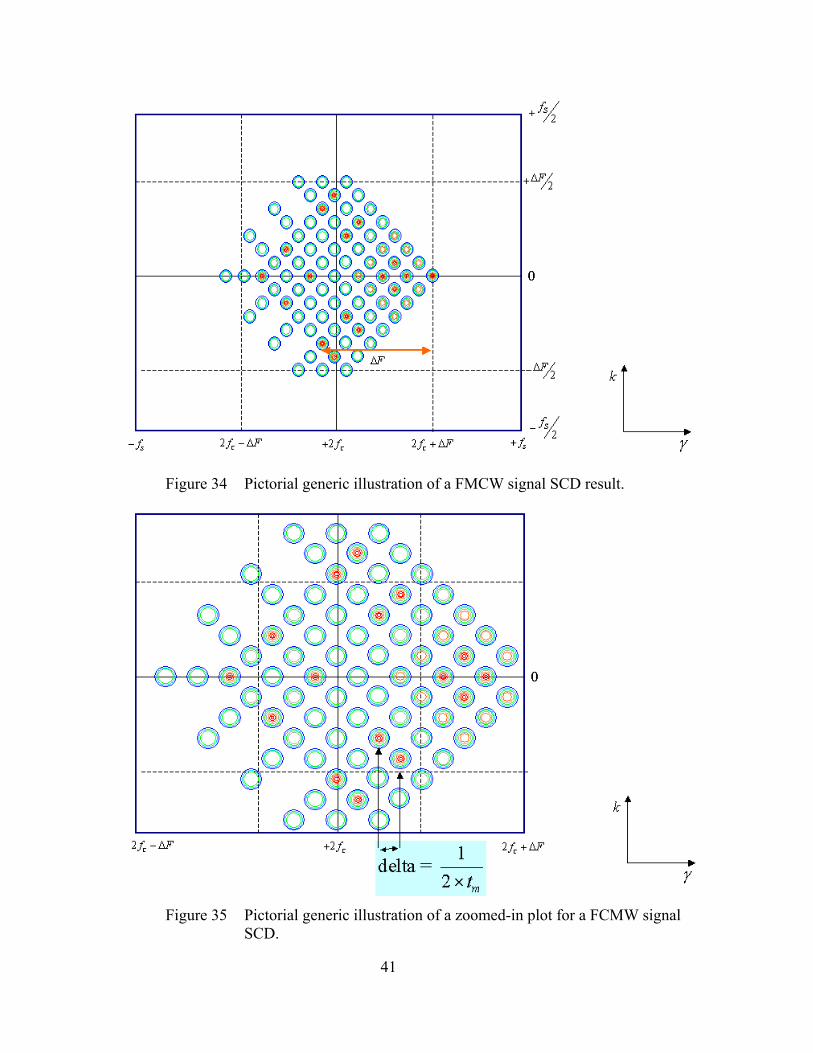
41
Figure 34 Pictorial generic illustration of a FMCW signal SCD result.
Figure 35 Pictorial generic illustration of a zoomed-in plot for a FCMW signal
SCD.

42
This secondary variable called “delta” is related to the modulation period as
shown in Figure 35 and in the examples of Figure 36 and Figure 37. From Figure 36
(FAM SCD with 2048, 4 and 16N M k= = ∆ = ) and Figure 37 (Zoomed in plot of
Figure 36), we get the values:
• Carrier frequency (fC) = 1000 Hz (directly from plot);
• BW ( F delta∆ ± ) 250 25Hz Hz≈ ± ;
• 1 1 0.02 202 2 25= = = =⋅ ⋅mt s msdelta , where delta=25Hz;
Figure 36 FAM generated SCD plot for a FMCW signal (1000Hz carrier and
estimated modulation BW of 230 Hz).

43
Figure 37 Zoomed-in FAM generated SCD plot for a FMCW signal (“delta”
value of 25Hz). 4. P4:
The example signal characteristics are as following:
Carrier Frequency (fC) 1000 Hz
Sampling Frequency (fS) 7000 Hz
Number of Phases (Np) 16
SNR Only Signal
Number of Carrier Cycles per Phase (cpp) 1 Table 6. P4 signals characteristics.
Figure 38 and Figure 39 show FAM-generated SCD plots. We may see that the
carrier still appears at twice its value on the cycle frequency axis, where the pattern of
equally spaced points begins to become visible. Note the white box drawn around the
data showing the general shape of the SCD plot divided in channel pair regions. In Figure
39 we can see in detail the estimation of the code rate value (fb). Figure 40 shows the
estimation of the number of phases, as shown in a pictorial representation on Figure 31.

44
Figure 38 FAM-generated SCD plot for a P4 signal (1125Hz carrier and
estimated BW of 1000Hz).
Figure 39 Zoomed-in FAM-generated SCD plot for a P4 signal (with estimated
code rate (fb) of 66Hz).

45
Figure 40 Zoomed-in FAM-generated SCD plot for a P4 signal (with estimation
of BW and number of phases).
Therefore
• Carrier frequency (fC) = 1125Hz (directly from plot);
• Measured BW CfBW cpp =
1000 66Hz Hz≈ ± (therefore cpp=1);
• Number of Phases Used in the P4 Modulation (Np):
1000 15.15 16 phases66b
BW HzNp f Hz= = = ∼ ;
• Code Period (Tp): 1 16 0.0161000C
cpp NpTp sf⋅ ⋅= = = ; and
• Code Rate ( ) ( )1 1 62.50.016bf HzTp= = = .

46
C. CHAPTER SUMMARY
This chapter briefly discussed the theory related to the cyclostationarity concept.
Two computationally efficient cyclostationary processing algorithms (FAM and DFSM)
were discussed and their implementation in MATLAB® [4] was described.
The visual feature extraction was explained for some of the modulation types that
will be analyzed in the next chapter. The contour bi-frequency plots were chosen due to
their greatest contrast with the figure background and the convenient zooming capability
of MATLAB® [4] was explored to extract parameters such as: carrier frequency, code
rate and code period, BW, number of phases or number of Barker bits present on the
modulation and modulation period for the FMCW case. In the next section, the signal
matrix shown in Table 1 is analyzed and the theoretical values are compared with the
measurements from the SCD plots, according to the tutorial discussed in this chapter.

47
IV. DESCRIPTION OF LPI SPECTRAL PROPERTIES AND CYCLOSTATIONARY PROCESSING RESULTS
In this chapter we will analyze a set of LPI signals, with and without the addition
of White Gaussian Noise, and extract their main characteristics. All signals were
generated using the “LPI Generator” code from [5]. A detailed description of all
waveforms may be found in [5]. Table 8 shows the signal examples analyzed in this
chapter. SIGNAL NAME
CARRIER OR HOPPING
SEQUENCE (kHz)
BW (Hz)
NPBB/CPP
NUMBER OF BITS / PHASES
AND MOD.
PERIOD
MOD. TYPE
B_1_7_7_1_s.mat 1 1000 1 7 BPSK F_1_7_250_20_s.mat 1 250 X 20 FMCW
P1_1_7_4_1_s.mat 1 1000 1 16 P1 P2_1_7_16_1_s.mat 1 1000 1 16 P2 P3_1_7_16_1_s.mat 1 1000 1 16 P3 P4_1_7_16_1_s.mat 1 1000 1 16 P4 FR_1_7_16_1_s.mat 1 1000 1 16 FRANK
C_1_15_10_s.mat 4, 7, 1, 6, 5, 2, 3 - 10 1 COSTAS FSK_PSK_C_1_15_5_1_s.mat 4, 7, 1, 6, 5, 2, 3 1000 1 5 FSK/PSK COSTAS FSK_PSK_T_15_128_5_s.mat - 4200 5 128 Hops FSK/PSK TARGET
Table 7. List of signal examples analyzed in this thesis.
The signal analysis will consist of a brief theoretical description of the signals, an
illustration of the spectral properties using plots of the PSD, and the resulting plots from
the Cyclostationary processing algorithms discussed previously. Both time-smoothing
and frequency-smoothing methods will be used and the method that presents the best
visualization will be chosen for parameter extraction. The features extracted from the
signals will be presented in tables comparing the measured results with the given
parameters.

48
A. TEST SIGNALS
1. Description
The Test Signals were chosen to be single carrier signals with no modulation
• 1000Hz Single Carrier with 7000Hz Sampling Frequency;
• 1000Hz and 2000Hz Double Carrier with 7000Hz Sampling Frequency.
These signals give an insight on how the carrier frequency information may be extracted
from each plot.
2. Spectral Properties and Results (T_1_7_1_s and T_12_7_2_s)
Figure 41 shows the PSD of both Test Signals.
Figure 41 PSD plots for both Test signals: a) 1000Hz single sarrier and b) 1 and
2000Hz double carrier, no modulation.

49
The single carrier case is discussed on Chapter III. From Figure 42 and Figure 43
we can see that the SCD plots for the real part of the double carrier signal show the inter-
modulation product at the average of both carrier frequencies (1500Hz) and at 500Hz.
Figure 42 DFSM generated estimated SCD for a Test signal (1000Hz and
2000Hz double carrier).
Figure 43 Zoomed in DFSM generated estimated SCD for a Test signal (1000
and 2000Hz double carrier).

50
Table 9 compares the measured and original characteristics.
Feature Extraction
Characteristic Original Measured
Carrier Frequency (fC) 1000Hz
2000Hz
1000Hz
2000Hz
1500Hz and 500Hz
(intermodulation products)
Sampling Frequency (fs) 7000Hz. given Table 8. Comparison between measured and original characteristics for the Test
signals.
The Frequency-Smoothing technique generated easier to visualize results, and for such
simple signals the performance is equivalent to the Time-Smoothing algorithm. A Time-
Smoothing generated plot is shown in Chapter III for the first Test Signal (1000Hz). The
time-smoothing results for the second test signal, with double carriers, are not shown
since they are very similar to the DFSM plots of Figure 42 and Figure 43.
B. BPSK
1. Description:
Binary Phase Shift Keying codes are not considered LPI radar waveforms in the
strict sense of the word, but they are here included as a guide or academic tool to
facilitate the visualization of the resulting outputs from each algorithm.
This type of signal consists basically of using Barker Sequences of various
lengths to perform a binary phase modulation of the carrier (0 and π ). The signal is then
sampled and the output of the generator is saved as two vectors (I and Q) representing the
in phase and quadrature components of the signal. The modulation is performed
following the block diagram on Figure 44 [5].

51
Idealsampler ∑~
13-bit Barker Code Sequence[ 1 1 1 1 1 –1 –1 1 1 –1 1 –1 1 ]
X
White Gaussian NoiseSNR set by user
x(t) x(nT) I w/ noiseISave data to file
Idealsampler ∑∑~
13-bit Barker Code Sequence[ 1 1 1 1 1 –1 –1 1 1 –1 1 –1 1 ]
X
White Gaussian NoiseSNR set by user
x(t) x(nT) I w/ noiseISave data to file
Figure 44 Block diagram for BPSK modulation (from [5]).
In this work, we are going to analyze a waveform modulated with a Barker
Sequence of length 7 bits, at various signal-to-noise ratios. All MATLAB® [4] plots were
generated with the “cyclo.m” generated GUI and using a frequency resolution of 16 Hz
that influence directly on how precise the measurements of the code rate ( bf ) are made.
The FAM SCD plots were estimated using N=2048 and M=4, the DFSM SCD plots were
estimated using N=1024 and M=2.
2. Spectral Properties and Results (B_1_7_7_1_s)
The first signal to be analyzed is a 7-Bit Barker Code phase modulated signal,
with carrier frequency at 1000Hz and with 1NPBB = . No noise is added at this moment
and the carrier presents a lower magnitude in the PSD plot meaning that this may be
called a “Suppressed Carrier Dual Side Band” (SC-DSB) Modulation. The first signal
analyzed has its characteristics defined on Table 10.
Name Carrier
Frequency
(fC)
Sampling
Frequency
(fS)
Number of
Barker Bits
(Np)
Number of Carrier
Periods per Barker Bit
(NPBB)
B_1_7_7_1_s 1000 Hz 7000 Hz 7 1
Table 9. B_1_7_7_1_s signal characteristics.
The following sequence of Figures give an overview of the frequency content (Figure 45)
and the Estimated SCD (Figure 46, Figure 47, Figure 48, Figure 49 and Figure 50) of the

52
signal analyzed. The blue background of the SCD estimation contour plots helps in
visually filtering out the noise.
Figure 45 PSD for a Barker signal (1000Hz carrier, 7-bits Barker sequence and
1 NPBB).
Figure 46 Estimated FAM SCD contour plot for a BPSK real signal with
1000Hz carrier, Barker-7 code and 1 NPBB.

53
Figure 47 Estimated FAM SCD contour plot for a BPSK real signal with
1000Hz carrier, Barker-7 code and 1 NPBB, with estimated carrier of 1000Hz and estimated BW of 1000Hz.
Figure 48 Zoomed-in FAM SCD contour plot for a BPSK signal with 1000Hz
carrier, Barker-7 code and 1 NPBB, with estimated bf of 141 Hz.

54
Figure 49 Estimated DFSM SCD contour plot for a BPSK signal with 1000Hz
carrier, Barker-7 code and 1 NPBB, with estimated BW of 1000Hz.
Figure 50 Zoomed-in estimated DFSM SCD contour plot for a BPSK signal
with 1000Hz carrier, Barker-7 code and NPBB = 1, with estimated bf of 142Hz.

55
Figures 51 to 55 include the analysis of the same signal with added White Gaussian
Noise. At the end of this analysis, a table is included comparing the original and the
measured characteristics of each signal.
Figure 51 PSD for a Barker signal (1000Hz carrier, 7-bits Barker sequence, 1
NPBB and 0 dB SNR).
Figure 52 Estimated FAM SCD contour plot for a BPSK signal with 1000Hz
carrier, 7-bits Barker code, 1 NPBB and 0 dB SNR, with estimated BW of 1000Hz.
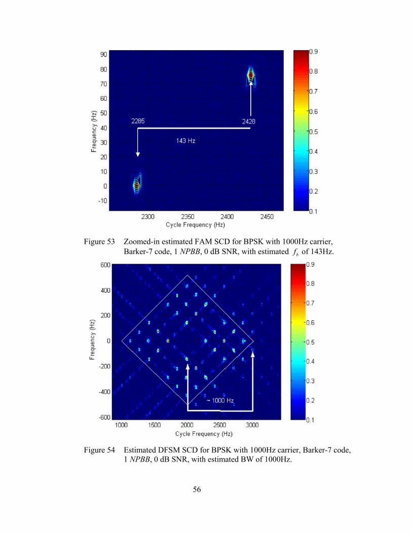
56
Figure 53 Zoomed-in estimated FAM SCD for BPSK with 1000Hz carrier,
Barker-7 code, 1 NPBB, 0 dB SNR, with estimated bf of 143Hz.
Figure 54 Estimated DFSM SCD for BPSK with 1000Hz carrier, Barker-7 code,
1 NPBB, 0 dB SNR, with estimated BW of 1000Hz.

57
Figure 55 Zoomed-in estimated FAM SCD for BPSK with 1000Hz carrier,
Barker-7 code, 1 NPBB, 0 dB SNR, with estimated bf of 144Hz.
The following table shows a comparison between the given and the measured
parameters.
Feature Extraction
Characteristic Original Measured
Carrier Frequency (fC) 1000 Hz 1000 Hz
Band Width (BW) 1000 Hz 997.5 Hz
Carrier Periods Per Barker Bit (NPBB) 1CfNPBB BW= = 1000 1.0025997.5NPBB = =
Code Rate ( bBWf k= ) 1000 142.87bf = = 142.75 Hz (average)
Number of Barker Bits (Np) 7b
BWk f= = 1000 7.005142.75k = =
Table 10. Comparison between measured and original characteristics for This BPSK signal.
The BPSK signals analyzed helped as an example in determining how to make
measurements in more complex signals such as FMCW, Polyphase and frequency
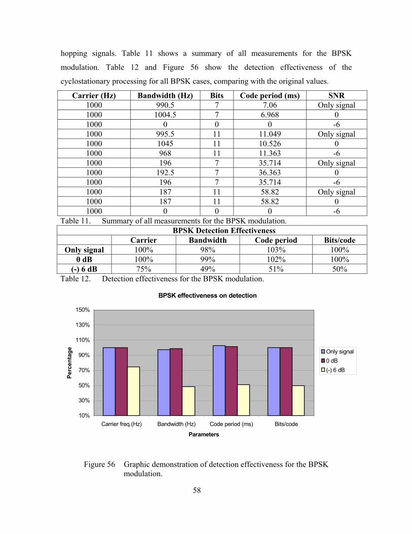
58
hopping signals. Table 11 shows a summary of all measurements for the BPSK
modulation. Table 12 and Figure 56 show the detection effectiveness of the
cyclostationary processing for all BPSK cases, comparing with the original values.
Carrier (Hz) Bandwidth (Hz) Bits Code period (ms) SNR 1000 990.5 7 7.06 Only signal 1000 1004.5 7 6.968 0 1000 0 0 0 -6 1000 995.5 11 11.049 Only signal 1000 1045 11 10.526 0 1000 968 11 11.363 -6 1000 196 7 35.714 Only signal 1000 192.5 7 36.363 0 1000 196 7 35.714 -6 1000 187 11 58.82 Only signal 1000 187 11 58.82 0 1000 0 0 0 -6
Table 11. Summary of all measurements for the BPSK modulation. BPSK Detection Effectiveness
Carrier Bandwidth Code period Bits/code Only signal 100% 98% 103% 100%
0 dB 100% 99% 102% 100% (-) 6 dB 75% 49% 51% 50%
Table 12. Detection effectiveness for the BPSK modulation.
BPSK effectiveness on detection
10%
30%
50%
70%
90%
110%
130%
150%
Carrier freq.(Hz) Bandwidth (Hz) Code period (ms) Bits/code
Parameters
Perc
enta
ge Only signal0 dB(-) 6 dB
Figure 56 Graphic demonstration of detection effectiveness for the BPSK modulation.

59
C. FMCW
1. Description
The triangular modulation of a Frequency Modulated Continuous Wave (FMCW)
is very popular as a LPI application for a Continuous Wave signal. The emitter uses a
continuous 100% duty-cycle waveform and therefore, target range and Doppler
information can be measured unambiguously while retaining the LPI characteristics. The
FMCW signal is usually easier to implement than phase code modulation signals as long
as there is not strict demand on linearity over the modulation BW. [5] The triangular
modulation consists of two linear frequency modulation sections with positive and
negative slopes. With this configuration, the range and Doppler frequency of the detected
target can be extracted unambiguously by taking the sum and the difference of the two
beat frequencies. These characteristics are showed in Figure 57.
Figure 57 Linear Frequency Modulated Triangular Waveform and Doppler Shifted Signal [5]
2
dVfλ
=
Doppler shifted receiver signal
Transmitted signal
1b d dm
Ff f tt∆
= +
2b d dm
Ff f tt∆
= −

60
The frequency of the transmitted signal may calculated by
1 0( )2 m
F Ff t f tt
∆ ∆= − + (4.3.1)
for 0 < t < tm and zero elsewhere. Here f0 stands for RF carrier, ∆F stands for transmitted
modulation BW, and tm stands for modulation period. The rate of the frequency change or
chirp rate F is [5]
m
FFt∆
= (4.3.2)
The following section shows that we can measure these characteristics of an FMCW
signal in the bi-frequency plane generated by the cyclostationary algorithms
implemented.
2. Spectral Properties and Results (F_1_7_250_20_s)
This FMCW signal to be analyzed has a modulation period of 20 ms, with carrier
frequency at 1000Hz and modulation BW of 250 Hz. The signal has its characteristics
defined on Table 14:
Name Carrier
Frequency
(fC)
Sampling
Frequency
(fS)
Modulation
BW
(∆F)
Modulation Period
(tm)
F_1_7_250_20_s 1000 Hz 7000 Hz 250 Hz 20 ms
Table 13. F_1_7_250_20_s signal characteristics.
The PSD is shown in Figure 58 and shows the frequency content of the first FMCW
signal. The following sequence of Figures gives an overview of the frequency content
(Figure 58), time X frequency plot (Figure 59), and the Estimated SCD (Figure 60,
Figure 61, Figure 62 and Figure 63, all with N = 2048, frequency resolution of 16 Hz and
M = 4) of the signal analyzed.
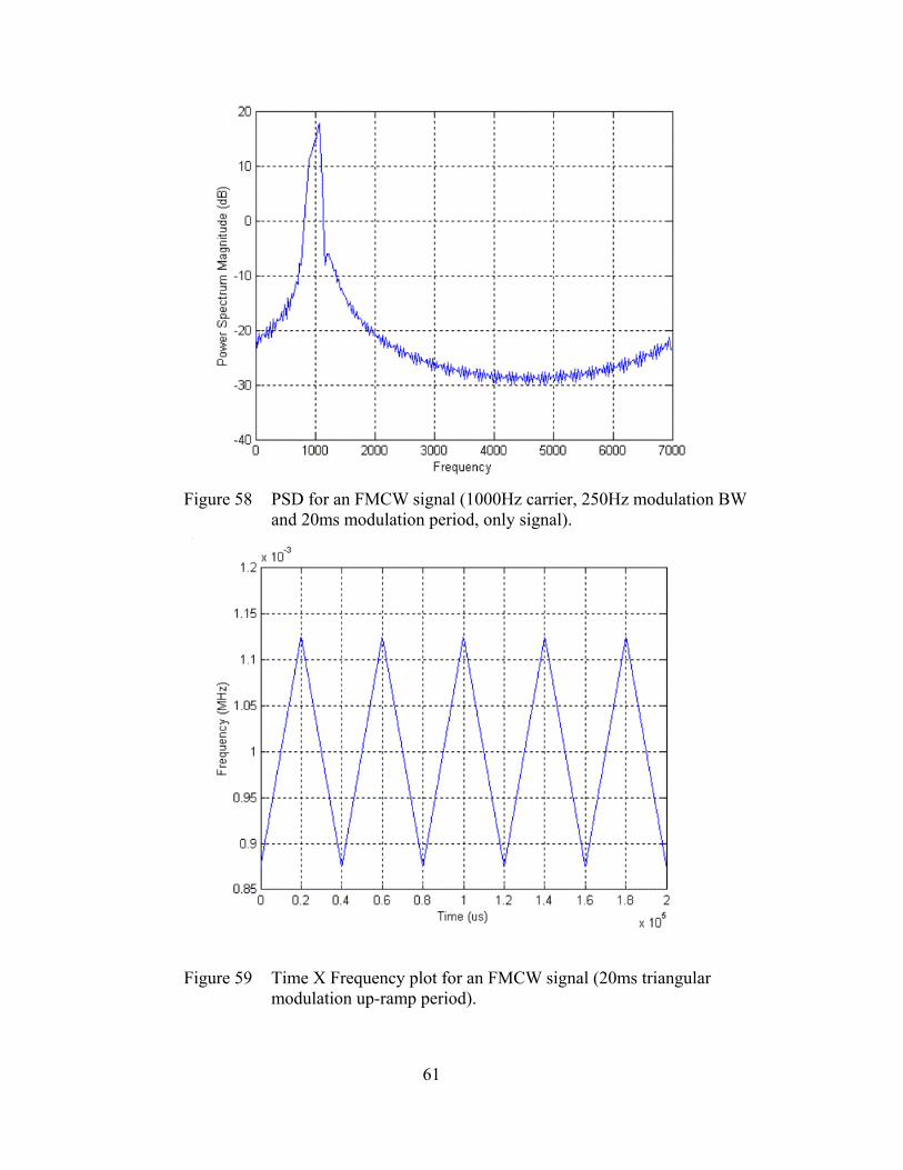
61
Figure 58 PSD for an FMCW signal (1000Hz carrier, 250Hz modulation BW
and 20ms modulation period, only signal).
Figure 59 Time X Frequency plot for an FMCW signal (20ms triangular
modulation up-ramp period).
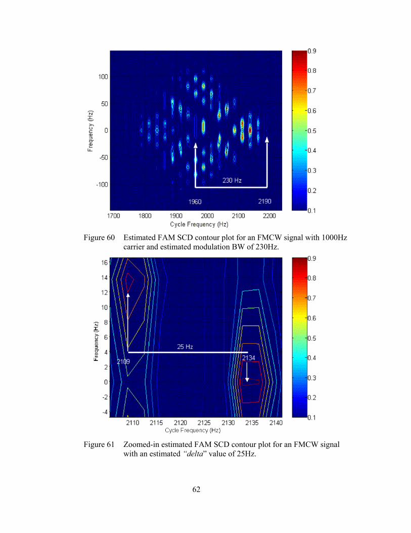
62
Figure 60 Estimated FAM SCD contour plot for an FMCW signal with 1000Hz
carrier and estimated modulation BW of 230Hz.
Figure 61 Zoomed-in estimated FAM SCD contour plot for an FMCW signal
with an estimated “delta” value of 25Hz.

63
Figure 62 Estimated DFSM SCD contour plot for an FMCW signal with
1000Hz carrier and estimated modulation BW of 235Hz.
Figure 63 Zoomed-in estimated DFSM SCD contour plot for an FMCW signal
with an estimated “delta” value of 21Hz.
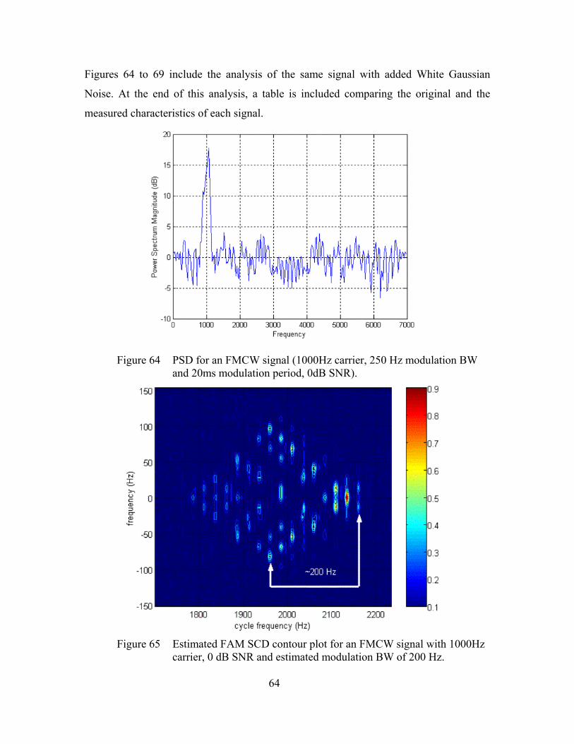
64
Figures 64 to 69 include the analysis of the same signal with added White Gaussian
Noise. At the end of this analysis, a table is included comparing the original and the
measured characteristics of each signal.
Figure 64 PSD for an FMCW signal (1000Hz carrier, 250 Hz modulation BW
and 20ms modulation period, 0dB SNR).
Figure 65 Estimated FAM SCD contour plot for an FMCW signal with 1000Hz
carrier, 0 dB SNR and estimated modulation BW of 200 Hz.

65
Figure 66 Estimated FAM SCD contour plot for an FMCW signal with an
estimated “delta” value of 26Hz.
Figure 67 PSD for an FMCW signal (1000Hz carrier, 250 Hz modulation BW
and 20ms modulation period, -6dB SNR).

66
Figure 68 Estimated FAM SCD contour plot for an FMCW signal with 1000Hz
carrier, -6 dB SNR and estimated modulation BW of 200 Hz.
Figure 69 Estimated FAM SCD contour plot for an FMCW signal with an
estimated “delta” value of 27Hz.

67
Table 15 shows that the main parameters of the FMCW modulation may be easily
measured in the bi-frequency plane, using both time and frequency-smoothing methods.
Feature Extraction
Characteristic Original Measured
Carrier Frequency (fC)
1000 Hz 992.83 Hz (average)
Modulation BW (∆F) 250 Hz 218.83 Hz
“Delta” 25 Hz 24.75 Hz (average)
Triangular Modulation Up-Ramp
Period (tm)
1 202*mt msdelta= = 1 0.02020 20.202*24.75mt s ms= = =
Table 14. Comparison between measured and original characteristics for an FMCW signal.
Table 16 shows a summary of all measurements for the FMCW modulation. Table 17 and
graphics on Figure 70 show the detection effectiveness of the cyclostationary processing
for the FMCW case, comparing with the original values.
Carrier (Hz) Modulation BW (Hz) Modulation Period (ms) SNR 992.5 232.5 21.74 Only signal 993 208 19.23 0 993 216 18.52 -6
987.5 221 29.42 Only signal 987.5 234 27.77 0 985 218.72 0 -6 970 470 20.83 Only signal 970 460 17.85 0 970 480 17.86 -6 978 470 33.33 Only signal 978 450 35.71 0 970 480 0 -6
Table 15. Summary of all measurements for the FMCW modulation. FMCW Detection Effectiveness
Carrier Modulation Bandwidth Modulation Period Only signal 98% 92% 106%
0 dB 98% 90% 99% (-) 6 dB 98% 91% 45%
Table 16. Detection effectiveness for the FMCW modulation.
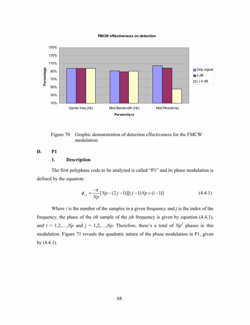
68
FMCW effectiveness on detection
10%
30%
50%
70%
90%
110%
130%
150%
Carrier freq.(Hz) Mod.Bandw idth (Hz) Mod.Period(ms)
Parameters
Perc
enta
ge Only signal
0 dB
(-) 6 dB
Figure 70 Graphic demonstration of detection effectiveness for the FMCW modulation.
D. P1
1. Description
The first polyphase code to be analyzed is called “P1” and its phase modulation is
defined by the equation:
, [ (2 1)][( 1) ( 1)]i j Np j j Np iNpπφ −
= − − − + − (4.4.1)
Where i is the number of the samples in a given frequency and j is the index of the
frequency, the phase of the ith sample of the jth frequency is given by equation (4.4.1),
and i = 1,2,…,Np and j = 1,2,…,Np. Therefore, there’s a total of Np2 phases in this
modulation. Figure 71 reveals the quadratic nature of the phase modulation in P1, given
by (4.4.1).

69
Figure 71 P1 code phase shift.
2. Spectral Properties and Results (P1_1_7_16_1_s)
This P1 signal has the following given characteristics:
Name Carrier
Frequency
(fC)
Sampling
Frequency
(fS)
Number of
Phases
(Np2)
Number of Cycles per
Phase (cpp)
P1_1_7_16_1_s 1000 Hz 7000 Hz 16 1
Table 17. P1_1_7_16_1_s signal characteristics.
Based on these properties, we expect a BW of 1000Hz, and yields from (4.4.1) that the
total number of phases is equal to Np2 and in this case, the 16 equally spaced regions
inside the BW are going to be separated by ( )2
1000 62.516bBWf Hz
Np= = = in the
cycle frequency axis. The PSD is shown in Figure 72 and shows the frequency content of
This P1 signal. The following sequence of Figures give an overview of the frequency
content (Figure 72) and the Estimated SCD (Figure 73 and Figure 74, with N = 1024,
frequency resolution of 16 Hz and M = 2) of the signal analyzed.

70
Figure 72 PSD for a P1 signal (1000Hz carrier, 16 phases and 1 cpp, only
signal).
Figure 73 Estimated DFSM SCD contour plot for a P1 signal with 900Hz carrier
and estimated BW of 1000Hz.
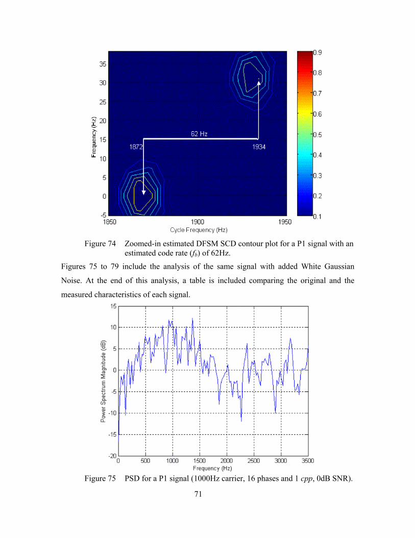
71
Figure 74 Zoomed-in estimated DFSM SCD contour plot for a P1 signal with an
estimated code rate (fb) of 62Hz.
Figures 75 to 79 include the analysis of the same signal with added White Gaussian
Noise. At the end of this analysis, a table is included comparing the original and the
measured characteristics of each signal.
Figure 75 PSD for a P1 signal (1000Hz carrier, 16 phases and 1 cpp, 0dB SNR).

72
Figure 76 Estimated FAM SCD contour plot for a P1 signal with 900Hz carrier
and estimated BW of 1000Hz, with 0dB SNR.
Figure 77 Zoomed-in estimated FAM SCD contour plot for a P1 signal with an
estimated code rate (fb) of 65Hz, with 0dB SNR.

73
Figure 78 PSD for a P1 signal (1000Hz carrier, 16 phases and 1 cpp, -6dB
SNR).
Figure 79 Estimated FAM SCD contour plot for a P1 signal with 850Hz carrier
and estimated BW of 1000Hz, with -6dB SNR.

74
The FAM measurements could be performed until an SNR of –6dB, except for the
bf value. All results from the DFSM processing were similar.
Feature Extraction
Characteristic Original Measured
Carrier Frequency (fC)
1000 Hz 876.67 Hz (average)
Bandwidth (BW)
1000 Hz 1000 Hz
Code Rate (fb) 62.5 Hz 63.5 Hz (average)
Number of Phases (Np2)
( )2 1000 1662.5b
BWNp f= = = ( )2 1000 15.7563.5b
BWNp f= = =
Code Period (tp)
1 0.016pb
t sf= = 1 1 0.0157563.5pb
t sf= = =
Table 18. Comparison between measured and original characteristics for a P1 signal.
Both time and frequency-smoothing processing techniques are very well suited for
analyzing high BW and short code period signals. Table 20 shows a summary of all
measurements for the P1 modulation.
Carrier (Hz) Bandwidth (Hz) Number of Phases Code period (ms) SNR 890 1000 4 16.13 Only signal870 1000 4 15.38 0 870 1000 0 0 -6 986 224 4 71.43 Only signal986 210 4 71.43 0 986 200 0 0 -6 986 1088 8 58.82 Only signal975 990 8 66.67 0 990 0 0 0 -6 1000 200 8 312.5 Only signal1000 200 8 250 0
0 0 0 0 -6 Table 19. Summary of all measurements for the P1 modulation.
Table 21 and graphics on Figure 80 show the detection effectiveness of the
cyclostationary processing for the P1 case, comparing with the original values for all the
P1 signals analyzed.
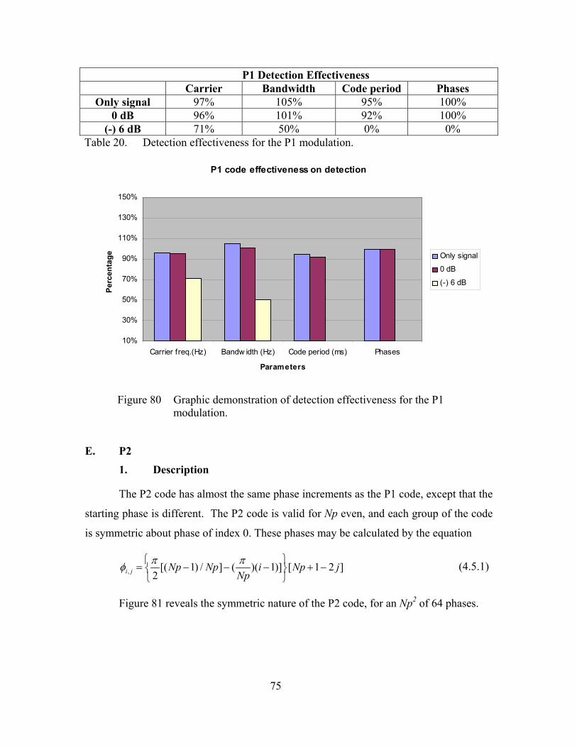
75
P1 Detection Effectiveness Carrier Bandwidth Code period Phases
Only signal 97% 105% 95% 100% 0 dB 96% 101% 92% 100%
(-) 6 dB 71% 50% 0% 0% Table 20. Detection effectiveness for the P1 modulation.
P1 code effectiveness on detection
10%
30%
50%
70%
90%
110%
130%
150%
Carrier freq.(Hz) Bandw idth (Hz) Code period (ms) Phases
Parameters
Perc
enta
ge Only signal
0 dB
(-) 6 dB
Figure 80 Graphic demonstration of detection effectiveness for the P1
modulation.
E. P2
1. Description
The P2 code has almost the same phase increments as the P1 code, except that the
starting phase is different. The P2 code is valid for Np even, and each group of the code
is symmetric about phase of index 0. These phases may be calculated by the equation
, [( 1) / ] ( )( 1)] [ 1 2 ]2i j Np Np i Np j
Npπ πφ
= − − − + −
(4.5.1)
Figure 81 reveals the symmetric nature of the P2 code, for an Np2 of 64 phases.
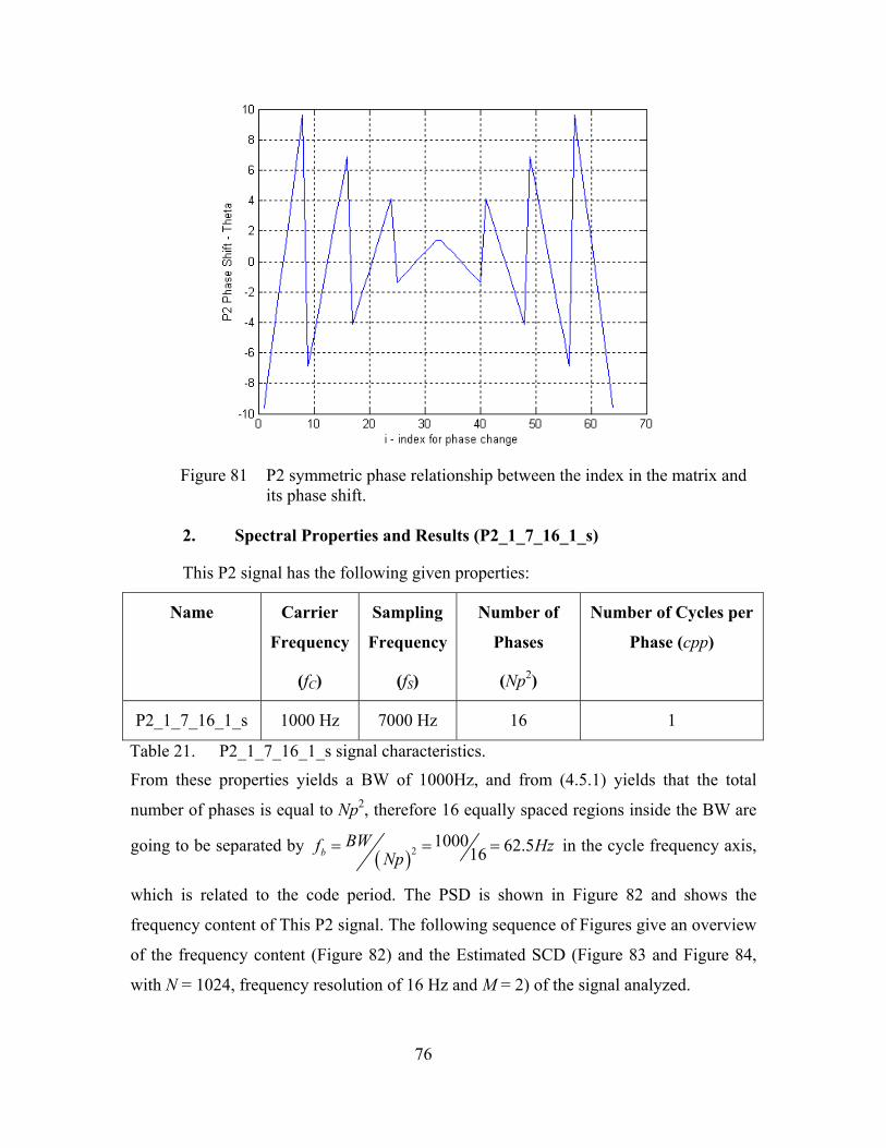
76
Figure 81 P2 symmetric phase relationship between the index in the matrix and
its phase shift. 2. Spectral Properties and Results (P2_1_7_16_1_s)
This P2 signal has the following given properties:
Name Carrier
Frequency
(fC)
Sampling
Frequency
(fS)
Number of
Phases
(Np2)
Number of Cycles per
Phase (cpp)
P2_1_7_16_1_s 1000 Hz 7000 Hz 16 1
Table 21. P2_1_7_16_1_s signal characteristics.
From these properties yields a BW of 1000Hz, and from (4.5.1) yields that the total
number of phases is equal to Np2, therefore 16 equally spaced regions inside the BW are
going to be separated by ( )2
1000 62.516bBWf Hz
Np= = = in the cycle frequency axis,
which is related to the code period. The PSD is shown in Figure 82 and shows the
frequency content of This P2 signal. The following sequence of Figures give an overview
of the frequency content (Figure 82) and the Estimated SCD (Figure 83 and Figure 84,
with N = 1024, frequency resolution of 16 Hz and M = 2) of the signal analyzed.
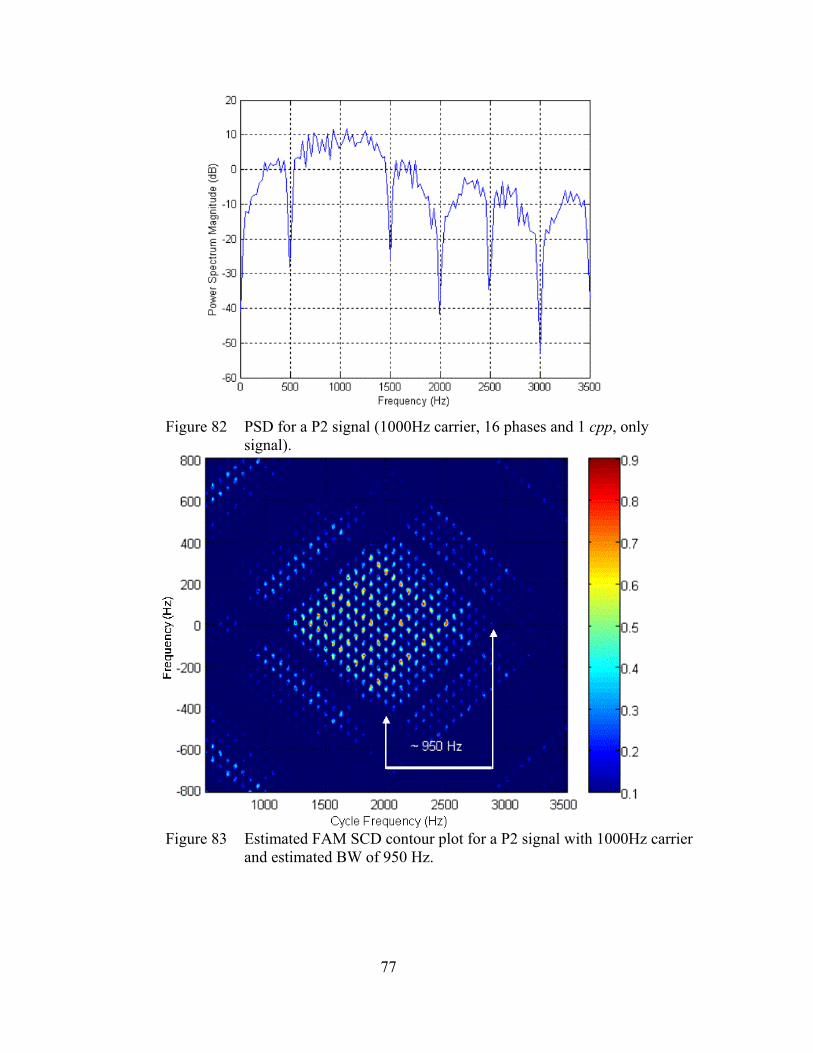
77
Figure 82 PSD for a P2 signal (1000Hz carrier, 16 phases and 1 cpp, only
signal).
Figure 83 Estimated FAM SCD contour plot for a P2 signal with 1000Hz carrier
and estimated BW of 950 Hz.

78
Figure 84 Zoomed-in estimated FAM SCD contour plot for a P2 signal with an
estimated code rate (fb) of 65 Hz.
Figures 85 to 87 include the analysis of the same signal with added White Gaussian
Noise. At the end of this analysis, a table is included comparing the original and the
measured characteristics of each signal.
Figure 85 PSD for a P2 signal (1000Hz carrier, 16 phases and 1 cpp, 0dB SNR).

79
Figure 86 Estimated DSFM SCD contour plot for a P2 signal with 1000Hz
carrier and estimated BW of 850Hz, with 0dB SNR.
Figure 87 Zoomed-in estimated DFSM SCD contour plot for a P2 signal with an
estimated code rate (fb) of 65Hz, with 0dB SNR.

80
The results are summarized in Table 23.
Feature Extraction
Characteristic Original Measured
Carrier Frequency (fC)
1000 Hz 1015 Hz (average)
Bandwidth (BW)
1000 Hz 900 Hz (average)
Code Rate (fb) 62.5 Hz 65 Hz (average)
Number of Phases (Np2)
( )2 1000 1662.5b
BWNp f= = = ( )2 900 13.8465b
BWNp f= = =
Code Period (tp) 1 0.016pb
t sf= = 1 1 0.0153865pb
t sf= = =
Table 22. Comparison between measured and original characteristics for a P2 signal.
Table 24 shows a summary of all measurements for the P2 modulation.
Carrier (Hz) Bandwidth (Hz) Number of Phases Code period (ms) SNR 1000 975 3.873 15.38 Only signal1030 870 3.66 15.38 0
0 0 0 0 -6 1000 167.5 3.52 74.07 Only signal1007 180 3.59 71.43 0 1000 150 0 0 -6 1000 962 8.28 71.43 Only signal1100 1100 4.5 18.2 0 1050 1200 0 0 -6 975 195 0 0 Only signal1000 175 0 0 0 970 240 0 0 -6
Table 23. Summary of all measurements for the P2 modulation.
Table 25 and graphics on Figure 88 show the detection effectiveness of the
cyclostationary processing for the P2 case, comparing with the original values.
P2 Detection Effectiveness Carrier Bandwidth Code period Phases
Only signal 99% 94% 75% 72% 0 dB 103% 94% 53% 59%
(-) 6 dB 76% 79% 0% 0% Table 24. Detection effectiveness for the P2 modulation.
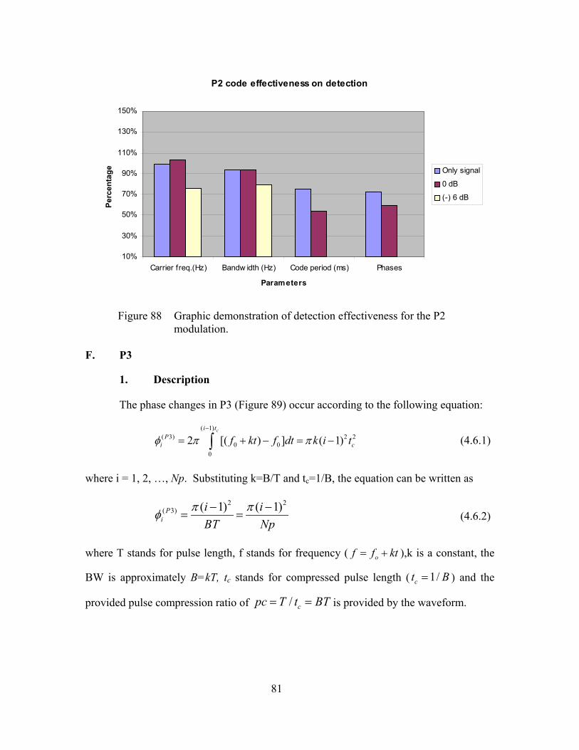
81
P2 code effectiveness on detection
10%
30%
50%
70%
90%
110%
130%
150%
Carrier freq.(Hz) Bandw idth (Hz) Code period (ms) Phases
Parameters
Perc
enta
ge Only signal
0 dB
(-) 6 dB
Figure 88 Graphic demonstration of detection effectiveness for the P2
modulation.
F. P3
1. Description
The phase changes in P3 (Figure 89) occur according to the following equation:
( 1)( 3) 2 2
0 00
2 [( ) ] ( 1)ci t
Pi cf kt f dt k i tφ π π
−
= + − = −∫ (4.6.1)
where i = 1, 2, …, Np. Substituting k=B/T and tc=1/B, the equation can be written as
2 2( 3) ( 1) ( 1)Pi
i iBT Np
π πφ − −= = (4.6.2)
where T stands for pulse length, f stands for frequency ( of f kt= + ),k is a constant, the
BW is approximately B=kT, tc stands for compressed pulse length ( 1/ct B= ) and the
provided pulse compression ratio of / cpc T t BT= = is provided by the waveform.
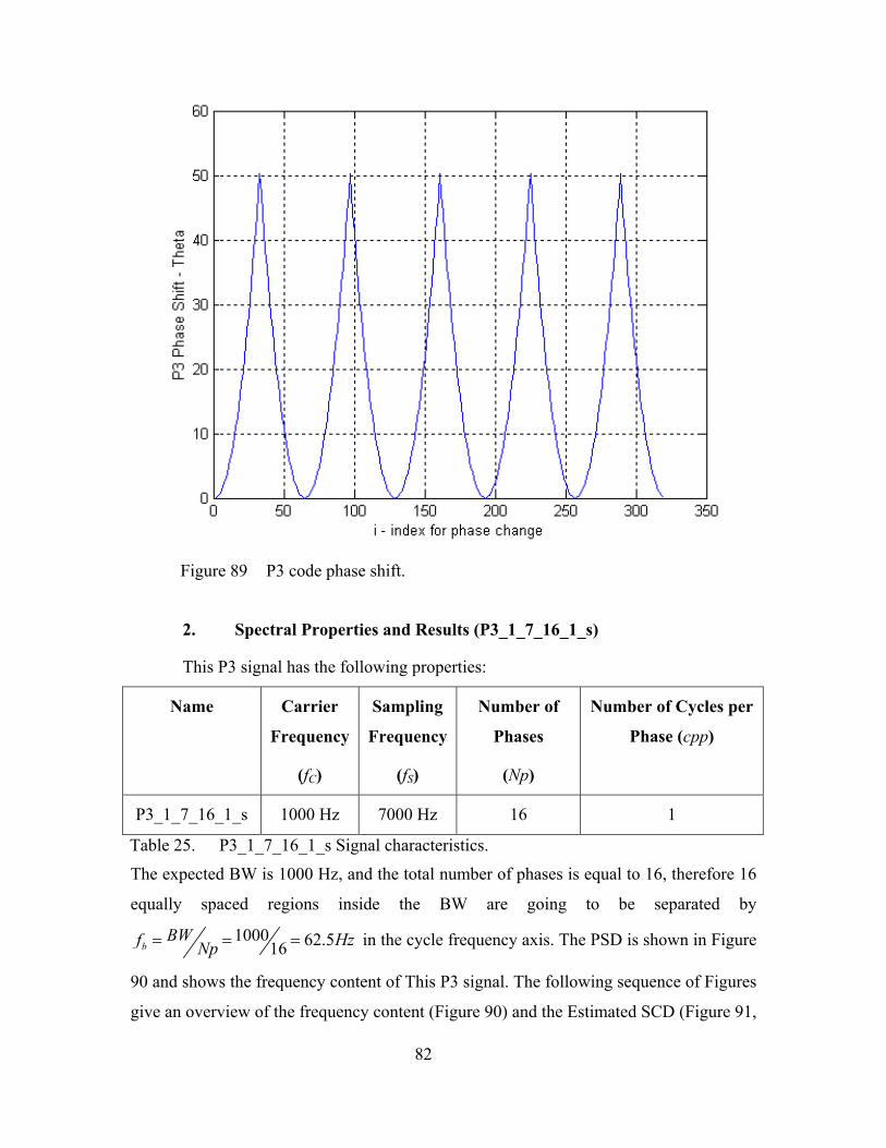
82
Figure 89 P3 code phase shift.
2. Spectral Properties and Results (P3_1_7_16_1_s)
This P3 signal has the following properties:
Name Carrier
Frequency
(fC)
Sampling
Frequency
(fS)
Number of
Phases
(Np)
Number of Cycles per
Phase (cpp)
P3_1_7_16_1_s 1000 Hz 7000 Hz 16 1
Table 25. P3_1_7_16_1_s Signal characteristics.
The expected BW is 1000 Hz, and the total number of phases is equal to 16, therefore 16
equally spaced regions inside the BW are going to be separated by
1000 62.516bBWf HzNp= = = in the cycle frequency axis. The PSD is shown in Figure
90 and shows the frequency content of This P3 signal. The following sequence of Figures
give an overview of the frequency content (Figure 90) and the Estimated SCD (Figure 91,

83
Figure 92, Figure 93 and Figure 94, with N = 1024, frequency resolution of 16 Hz and M
= 2) of the signal analyzed.
Figure 90 PSD for a P3 signal (1000Hz carrier, 16 phases and 1 cpp, only
signal).
Figure 91 Estimated FAM SCD contour plot for a P3 signal with 1100Hz carrier
and estimated BW of 1000Hz.

84
Figure 92 Zoomed-in estimated FAM SCD contour plot for a P3 signal with an
estimated fb of 62 Hz.
Figure 93 Estimated DFSM SCD contour plot for a P3 signal with 1150Hz
carrier and estimated BW of 1000Hz.
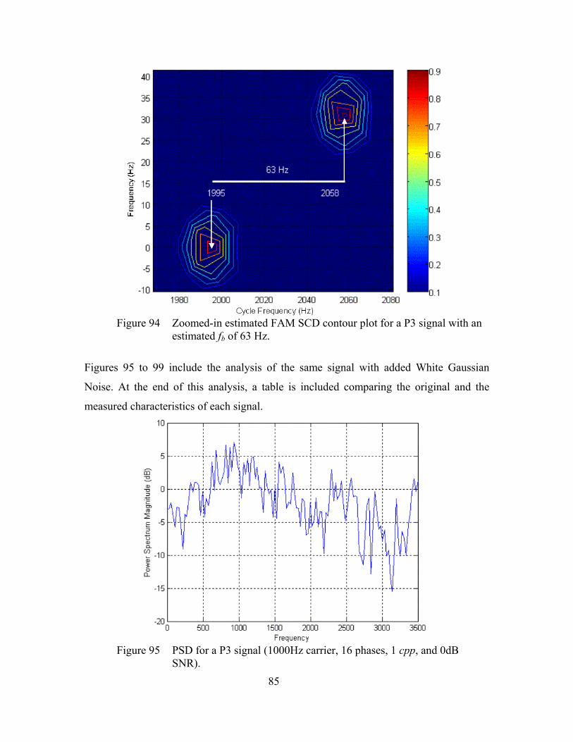
85
Figure 94 Zoomed-in estimated FAM SCD contour plot for a P3 signal with an
estimated fb of 63 Hz.
Figures 95 to 99 include the analysis of the same signal with added White Gaussian
Noise. At the end of this analysis, a table is included comparing the original and the
measured characteristics of each signal.
Figure 95 PSD for a P3 signal (1000Hz carrier, 16 phases, 1 cpp, and 0dB
SNR).

86
Figure 96 Estimated FAM SCD contour plot for a P3 signal with 1050Hz carrier
and estimated BW of 1000Hz, with 0dB SNR.
Figure 97 Zoomed-in estimated FAM SCD contour plot for a P3 signal with an
estimated fb of 56 Hz and 0dB SNR.

87
Figure 98 Estimated DFSM SCD contour plot for a P3 signal with 1050Hz
carrier and estimated BW of 1000Hz, with 0dB SNR.
Figure 99 Zoomed-in estimated DFSM SCD contour plot for a P3 signal with an
estimated fb of 68 Hz and 0dB SNR.

88
The given and measured features are summarized in Table 27.
Feature Extraction
Characteristic Original Measured
Carrier Frequency (fC)
1000 Hz 1075 Hz
Bandwidth (BW)
1000 Hz 1000 Hz
Code Rate (fb) 62.5 Hz 62 Hz (average)
Number of Phases (Np)
1000 1662.5b
BWNp f= = = 1000 16.1362b
BWNp f= = =
Code Period (tp)
1 0.016pb
t sf= = 1 0.01612962pt s= =
Table 26. Comparison between measured and original characteristics for a P3 signal.
Table 28 shows a summary of all measurements for the P3 modulation.
Carrier (Hz) Bandwidth (Hz) Number of Phases Code period (ms) SNR 1100 1000 16.01 16 Only signal1050 1000 16.03 16 0
0 0 0 0 -6 1000 200 14.71 71.43 Only signal1000 200 14.71 71.43 0 1000 220 0 0 -6 1100 1000 71.43 71.43 Only signal1000 1000 71.43 71.43 0
0 0 0 0 -6 1000 200 7.143 35.71 Only signal1000 200 7.143 35.71 0
0 0 0 0 -6 Table 27. Summary of all measurements for the P3 modulation.
Table 29 and graphics on Figure 100 show the detection effectiveness of the
cyclostationary processing for the P3 case, comparing with the original values.
P3 Detection Effectiveness Carrier Bandwidth Code period Phases
Only signal 105% 100% 78% 79% 0 dB 101% 100% 78% 79%
(-) 6 dB 25% 28% 0% 0% Table 28. Detection effectiveness for the P3 modulation.

89
P3 code effectiveness on detection
10%
30%
50%
70%
90%
110%
130%
150%
Carrier freq.(Hz) Bandw idth (Hz) Code period (ms) Phases
Parameters
Perc
enta
ge Only signal
0 dB
(-) 6 dB
Figure 100 Graphic demonstration of detection effectiveness for the P3
modulation.
G. P4
1. Description
The P4 code is derived from the same waveform as the P3 code. However, in this
case, the LO frequency is set equal to / 2of kT+ in the I-Q detectors. With this
frequency, the phases of successive samples are defined by the equations: [5]
( 1) ( 1)( 4)
0 00 0
2 [( ) / 2] 2 ( / 2)c ci t i t
Pi f kt f kT dt k t T dtφ π π
− −
= + − + = −∫ ∫ (4.7.1)
2( 4) 2 2 ( 1)( 1) ( 1) ( 1)Pi c c
n ink i t nkT i t iNp
φ π −
= − − − = − −
(4.7.2)
Figure 101 shows the relationship between the index in the matrix and its subsequent
phase for a P4-coded signal with Np= 64 (phases).

90
Figure 101 Phase shift for a P4-coded signal with Np=64 phases
2. Spectral Properties and Results (P4_1_7_16_1_s)
The P4 signal has the following characteristics:
Name Carrier
Frequency
(fC)
Sampling
Frequency
(fS)
Number of
Phases
(Np)
Number of Cycles per
Phase (cpp)
P4_1_7_16_1_s 1000 Hz 7000 Hz 16 1
Table 29. P4_1_7_16_1_s signal characteristics.
The expected BW is 1000 Hz, and the total number of phases is equal to 16. There will be
16 equally spaced regions inside the BW separated by 1000 62.516bBWf HzNp= = = in
the cycle frequency axis. The PSD is shown in Figure 102 and shows the frequency
content of This P4 signal. The following sequence of Figures give an overview of the
frequency content (Figure 102) and the Estimated SCD (Figure 103, Figure 104, Figure

91
105, and Figure 106 with N = 1024, frequency resolution of 16 Hz and M = 2) of the
signal analyzed.
Figure 102 PSD for a P4 signal (1000Hz carrier, 16 phases and 1 cpp, only
signal).
Figure 103 Estimated FAM SCD contour plot for a P4 signal with 1100Hz carrier
and estimated BW of 1000 Hz.

92
Figure 104 Zoomed-in estimated FAM SCD contour plot for a P4 signal with an
estimated bf of 66 Hz.
Figure 105 Estimated DFSM SCD contour plot for a P4 signal with 1100Hz
carrier and estimated BW of 1000 Hz.

93
Figure 106 Zoomed-in estimated FAM SCD contour plot for a P4 signal with an
estimated bf of 62 Hz.
Figures 107 to 109 include the analysis of the same signal with added White Gaussian
Noise. At the end of this analysis, a table is included comparing the original and the
measured characteristics of each signal.
Figure 107 PSD for a P4 signal (1000Hz carrier, 16 phases, 1 cpp, and 0dB
SNR).

94
Figure 108 Estimated FAM SCD contour plot for a P4 signal with 1100Hz carrier
and estimated BW of 1000 Hz, with 0dB SNR.
Figure 109 Zoomed-in estimated FAM SCD contour plot for a P4 signal with an
estimated bf of 67 Hz, with 0dB SNR.

95
The given and measured features are summarized in the table below.
Feature Extraction
Characteristic Original Measured
Carrier Frequency (fC)
1000 Hz 1030 Hz (average)
Bandwidth (BW)
1000 Hz 1000 Hz
Code Rate (fb) 62.5 Hz 65.5 Hz (average)
Number of Phases (Np)
1000 1662.5b
BWNp f= = = 1000 15.2765.5b
BWNp f= = =
Code Period (tp)
1 0.016pb
t sf= = 1 0.0152765.5pt s= =
Table 30. Comparison between measured and original characteristics for a P4 signal.
Table 32 shows a summary of all measurements for the P4 modulation.
Carrier (Hz) Bandwidth (Hz) Number of Phases Code period (ms) SNR 1100 1000 15.625 16 Only signal1100 1000 14.93 16 0 1000 700 0 0 -6 1000 200 14.29 71.43 Only signal1000 200 14.29 71.43 0 960 120 0 0 -6 1000 1000 71.43 71.43 Only signal1000 1000 71.43 71.43 0 1000 1100 0 0 -6 1000 160 22.86 142.86 Only signal1000 170 12.59 74.1 0
0 0 0 0 -6 Table 31. Summary of all measurements for the P4 modulation.
Table 33 and graphics on Figure 110 show the detection effectiveness of the
cyclostationary processing for the P4 case, comparing with the original values.
P4 Detection Effectiveness Carrier Bandwidth Code period Phases
Only signal 103% 95% 86% 84% 0 dB 103% 96% 81% 78%
(-) 6 dB 74% 60% 0% 0% Table 32. Detection effectiveness for the P4 modulation.

96
P4 code effectiveness on detection
10%
30%
50%
70%
90%
110%
130%
150%
Carrier freq.(Hz) Bandw idth (Hz) Code period (ms) Phases
Parameters
Perc
enta
ge Only signal
0 dB
(-) 6 dB
Figure 110 Graphic demonstration of detection effectiveness for the P4 modulation.
H. FRANK
1. Description
Frank codes belong to the family of polyphase codes, Chirp codes and Barker
codes, and have been successfully used in implementing Low probability of Intercept
(LPI) radar signals. [5]
A Frank-coded waveform has a length of Np2 and basically consists of a constant
amplitude signal whose carrier frequency is modulated by the phases of the Frank code
given by the following equation:
,2 ( 1)( 1)i j i jNpπφ = − − (4.8.1)
where i = number of samples (i = 1,2… Np) and j = number of frequencies (j = 1,2,…
Np). Figure 111 clearly displays how the phases change in the Frank modulation.

97
Figure 111 Frank modulation phase changes Np2=16.
2. Spectral Properties and Results (FR_1_7_16_1_s)
This Frank signal has the following characteristics:
Name Carrier
Frequency
(fC)
Sampling
Frequency
(fS)
Number of
Phases
(Np2)
Number of Cycles per
Phase (cpp)
FR_1_7_16_1_s 1000 Hz 7000 Hz 16 1
Table 33. FR_1_7_16_1_s signal characteristics.
The expected BW is 1000 Hz, and the total number of phases is equal to 16. There will be
sixteen equally spaced regions inside the BW range separated by the distance
( )21000 62.516b
BWf HzNp
= = = in the cycle frequency axis. The PSD is shown in
Figure 112 and shows the frequency content of This Frank signal. The following
sequence of Figures give an overview of the frequency content (Figure 112) and the
Estimated SCD (Figure 113 and Figure 114, with N = 1024, frequency resolution of 16
Hz and M = 2) of the signal analyzed.

98
Figure 112 PSD for a Frank signal (1000Hz carrier, 16 phases and 1 cpp, only
signal).
Figure 113 Estimated DFSM SCD contour plot for a Frank signal with 1150Hz
carrier and estimated BW of 1000 Hz.

99
Figure 114 Zoomed-in estimated DFSM SCD contour plot for a Frank signal with
an estimated fb of 61 Hz.
Figures 115 to 120 include the analysis of the same signal with added White Gaussian
Noise. At the end of this analysis, a table is included comparing the original and the
measured characteristics of each signal.
Figure 115 PSD for a Frank signal (1000Hz carrier, 16 phases, 1 cpp, and 0dB
SNR).

100
Figure 116 Estimated FAM SCD contour plot for a Frank signal with 1000Hz
carrier and estimated BW of 1000 Hz, with 0dB SNR.
Figure 117 Zoomed-in estimated FAM SCD contour plot for a Frank signal with
an estimated fb of 63 Hz and 0dB SNR.
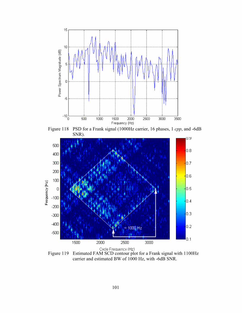
101
Figure 118 PSD for a Frank signal (1000Hz carrier, 16 phases, 1 cpp, and -6dB
SNR).
Figure 119 Estimated FAM SCD contour plot for a Frank signal with 1100Hz
carrier and estimated BW of 1000 Hz, with -6dB SNR.
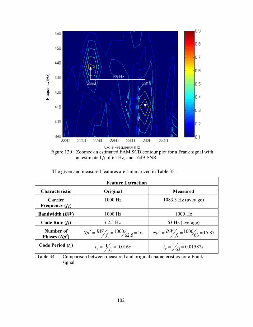
102
Figure 120 Zoomed-in estimated FAM SCD contour plot for a Frank signal with
an estimated fb of 65 Hz, and –6dB SNR.
The given and measured features are summarized in Table 35.
Feature Extraction
Characteristic Original Measured
Carrier Frequency (fC)
1000 Hz 1083.3 Hz (average)
Bandwidth (BW) 1000 Hz 1000 Hz
Code Rate (fb) 62.5 Hz 63 Hz (average)
Number of Phases (Np2)
2 1000 1662.5b
BWNp f= = = 2 1000 15.8763b
BWNp f= = =
Code Period (tp) 1 0.016pb
t sf= = 1 0.0158763pt s= =
Table 34. Comparison between measured and original characteristics for a Frank signal.
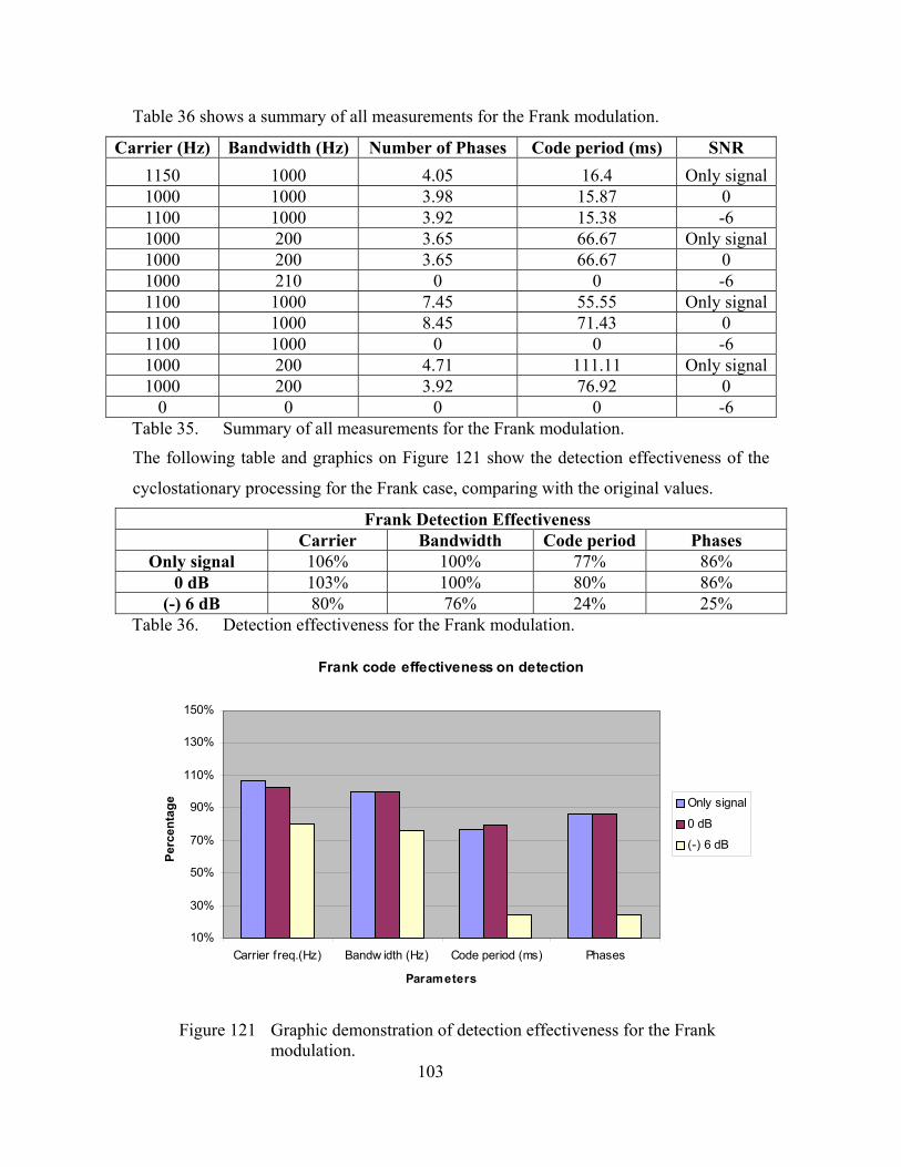
103
Table 36 shows a summary of all measurements for the Frank modulation.
Carrier (Hz) Bandwidth (Hz) Number of Phases Code period (ms) SNR 1150 1000 4.05 16.4 Only signal1000 1000 3.98 15.87 0 1100 1000 3.92 15.38 -6 1000 200 3.65 66.67 Only signal1000 200 3.65 66.67 0 1000 210 0 0 -6 1100 1000 7.45 55.55 Only signal1100 1000 8.45 71.43 0 1100 1000 0 0 -6 1000 200 4.71 111.11 Only signal1000 200 3.92 76.92 0
0 0 0 0 -6 Table 35. Summary of all measurements for the Frank modulation.
The following table and graphics on Figure 121 show the detection effectiveness of the
cyclostationary processing for the Frank case, comparing with the original values.
Frank Detection Effectiveness Carrier Bandwidth Code period Phases
Only signal 106% 100% 77% 86% 0 dB 103% 100% 80% 86%
(-) 6 dB 80% 76% 24% 25% Table 36. Detection effectiveness for the Frank modulation.
Frank code effectiveness on detection
10%
30%
50%
70%
90%
110%
130%
150%
Carrier freq.(Hz) Bandw idth (Hz) Code period (ms) Phases
Parameters
Perc
enta
ge Only signal
0 dB
(-) 6 dB
Figure 121 Graphic demonstration of detection effectiveness for the Frank
modulation.
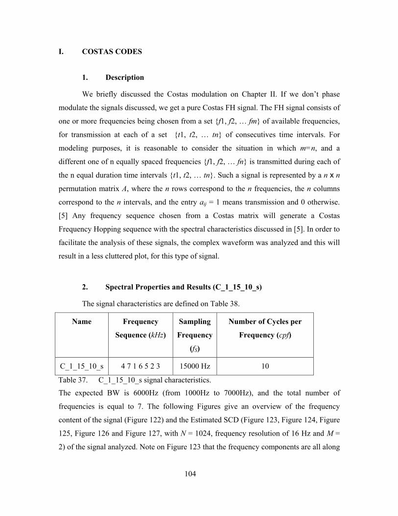
104
I. COSTAS CODES
1. Description
We briefly discussed the Costas modulation on Chapter II. If we don’t phase
modulate the signals discussed, we get a pure Costas FH signal. The FH signal consists of
one or more frequencies being chosen from a set {f1, f2, … fm} of available frequencies,
for transmission at each of a set {t1, t2, … tn} of consecutives time intervals. For
modeling purposes, it is reasonable to consider the situation in which m=n, and a
different one of n equally spaced frequencies {f1, f2, … fn} is transmitted during each of
the n equal duration time intervals {t1, t2, … tn}. Such a signal is represented by a n x n
permutation matrix A, where the n rows correspond to the n frequencies, the n columns
correspond to the n intervals, and the entry aij = 1 means transmission and 0 otherwise.
[5] Any frequency sequence chosen from a Costas matrix will generate a Costas
Frequency Hopping sequence with the spectral characteristics discussed in [5]. In order to
facilitate the analysis of these signals, the complex waveform was analyzed and this will
result in a less cluttered plot, for this type of signal.
2. Spectral Properties and Results (C_1_15_10_s)
The signal characteristics are defined on Table 38.
Name Frequency
Sequence (kHz)
Sampling
Frequency
(fS)
Number of Cycles per
Frequency (cpf)
C_1_15_10_s 4 7 1 6 5 2 3 15000 Hz 10
Table 37. C_1_15_10_s signal characteristics.
The expected BW is 6000Hz (from 1000Hz to 7000Hz), and the total number of
frequencies is equal to 7. The following Figures give an overview of the frequency
content of the signal (Figure 122) and the Estimated SCD (Figure 123, Figure 124, Figure
125, Figure 126 and Figure 127, with N = 1024, frequency resolution of 16 Hz and M =
2) of the signal analyzed. Note on Figure 123 that the frequency components are all along

105
the 0γ = axis (vertical or frequency axis) while the intermodulation products are located
symmetrically over the bi-frequency plane, outside the vertical axis.
Figure 122 PSD for a Costas signal (1, 2, 3, 4, 5, 6 and 7 kHz carriers, 10 cpf,
only signal).
Figure 123 Estimated FAM SCD contour plot for a complex Costas signal (1, 2,
3, 4, 5, 6 and 7000Hz carriers over 0γ = axis, cpf=10, only signal), with intermodulation products.

106
Figures 124 to 127 include the analysis of the same signal with added White Gaussian
Noise. At the end of this analysis, a table is included comparing the original and the
measured characteristics of each signal.
Figure 124 PSD for a Costas signal (1, 2, 3, 4, 5, 6 and 7kHz carriers, 10 cpf and
0dB SNR).
Figure 125 Estimated FAM SCD contour plot for a complex Costas signal (1, 2,
3, 4, 5, 6 and 7kHz carriers over 0γ = axis, 10 cpf, 0dB SNR), with intermodulation products.

107
Figure 126 PSD for a Costas signal (1, 2, 3, 4, 5, 6 and 7kHz carriers, 10 cpf and
SNR of -6dB).
Figure 127 Estimated FAM SCD contour plot for a complex Costas signal (1, 2,
3, 4, 5, 6 and 7kHz carriers over 0γ = axis, 10 cpf, -6dB SNR), with intermodulation products.

108
The order of the frequencies can’t be measured in this kind of plot since we don’t
have a “time x frequency” type of output, but the frequency content is easily determined.
Feature Extraction
Characteristic Original Measured
Frequency Components
1, 2, 3, 4, 5, 6 and 7kHz 1, 2, 3, 4, 5, 6 and 7kHz
BW (BW) 6000Hz 6000Hz Table 38. Comparison between measured and original characteristics for a Costas
signal.
The following table shows a summary of all measurements for the Costas modulation.
Sequence Time in each freq Code Period SNR 4 7 1 6 5 2 3 0 0 Only signal 4 7 1 6 5 2 3 0 0 0 4 7 1 6 5 2 3 0 0 -6 4 7 1 6 5 2 3 0 0 Only signal 4 7 1 6 5 2 3 0 0 0 4 7 1 6 5 2 3 0 0 -6 4 1 6 7 5 3 2 0 0 Only signal 4 1 6 7 5 3 2 0 0 0 4 1 6 7 5 3 2 0 0 -6 4 1 6 7 5 3 2 0 0 Only signal 4 1 6 7 5 3 2 0 0 0 4 1 6 7 5 3 2 0 0 -6
Table 39. Summary of all measurements for the Costas modulation.
The following table and graphics on Figure 128 show the detection effectiveness of the
cyclostationary processing for the Costas case, comparing with the original values.
Costas Detection Effectiveness Sequence Time in each Frequency Code period (ms)
Only signal 100% 0% 0% 0 dB 100% 0% 0%
(-) 6 dB 100% 0% 0% Table 40. Detection effectiveness for the Costas modulation.

109
Costas code effectiveness on detection
10%
30%
50%
70%
90%
110%
130%
150%
Sequence Time in frequency(ms) Code period (ms)
Parameters
Perc
enta
ge Only signal
0 dB
(-) 6 dB
Figure 128 Graphic demonstration of detection effectiveness for the Costas
modulation.
J. FSK/ PSK COSTAS
1. Description
A detailed description of this type of signal is given in Chapter II.
2. Spectral Properties and Results (FSK_PSK_C_1_15_5_1_s)
This FSK/PSK Costas signal has the following characteristics:
Name Frequency
Sequence
(kHz)
Sampling
Frequency
(fS)
Number of
Barker
Bits (Np)
Number of
Cycles per
Phase
(NPBB)
FSK_PSK_C_1_15_5_1_s 4 7 1 6 5 2 3 15000 Hz 5 1
Table 41. FSK_PSK_C_1_15_5_1_s signal characteristics.
The expected BW is 7000 Hz (from 500 Hz to 7.5kHz), each frequency will be
modulated with as BPSK Barker-5 and since the smallest frequency is 1000Hz, the BW
for each frequency hop will be 1000Hz. Inside each hop, we expect to see a
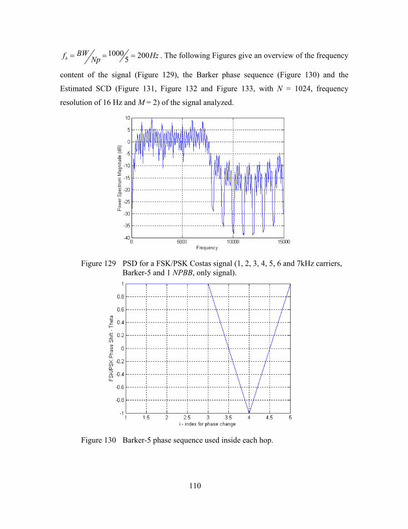
110
1000 2005bBWf HzNp= = = . The following Figures give an overview of the frequency
content of the signal (Figure 129), the Barker phase sequence (Figure 130) and the
Estimated SCD (Figure 131, Figure 132 and Figure 133, with N = 1024, frequency
resolution of 16 Hz and M = 2) of the signal analyzed.
Figure 129 PSD for a FSK/PSK Costas signal (1, 2, 3, 4, 5, 6 and 7kHz carriers,
Barker-5 and 1 NPBB, only signal).
Figure 130 Barker-5 phase sequence used inside each hop.

111
Figure 131 Estimated FAM SCD contour plot for a complex FSK/PSK Costas
signal (1, 2, 4, 5, 6 and 7kHz measured carriers).
Figure 132 Zoomed-in estimated FAM SCD contour plot for a complex
FSK/PSK Costas signal (4, 5 and 6kHz measured carriers and estimated BW of 1000 Hz for each frequency hop).

112
Figure 133 Estimated fb value of 200 Hz for the embedded Barker-5 BPSK
modulation.
Figures 134 to 137 include the analysis of the same signal with added White Gaussian
Noise. At the end of this analysis, a table is included comparing the original and the
measured characteristics of each signal.
Figure 134 PSD for a FSK/PSK Costas signal (1, 2, 3, 4, 5, 6 and 7kHz carriers,
Barker-5 and 1 NPBB, 0dB SNR).

113
Figure 135 Estimated FAM SCD contour plot for a complex FSK/PSK Costas
signal (1, 2, 4, 5, 6 and 7kHz measured carriers, 0dB SNR).
Figure 136 Zoomed-in estimated FAM SCD contour plot for a complex
FSK/PSK Costas signal (5, 6 and 7kHz measured carriers and estimated BW of 1000 Hz for each frequency hop, 0dB SNR).

114
Figure 137 Estimated fb value of 200 Hz for the embedded Barker-5 BPSK
modulation.
The given and measured features are summarized in the table below.
Feature Extraction
Characteristic Original Measured
Carrier Frequency (fc)
1, 2, 3, 4, 5, 6 and 7kHz 1, 4, 5, 6 and 7kHz
BW for Each Frequency Hop
(BW)
1000 Hz 1000 Hz
Code Rate (fb) 200 Hz 200 Hz
Number of Bits in Barker Code (Np)
1000 5200b
BWNp f= = = 1000 5200b
BWNp f= = =
Code Period Inside Each Hop
1 0.005pb
t sf= = 1 0.005200pt s= =
Table 42. Comparison between measured and original characteristics for a FSK/PSK Costas signal.
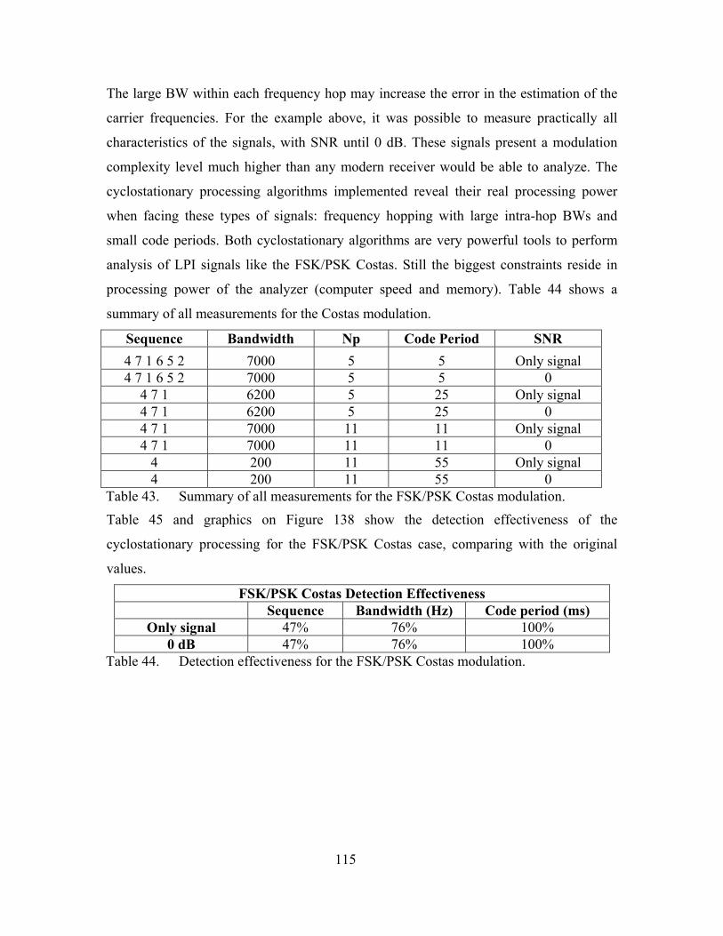
115
The large BW within each frequency hop may increase the error in the estimation of the
carrier frequencies. For the example above, it was possible to measure practically all
characteristics of the signals, with SNR until 0 dB. These signals present a modulation
complexity level much higher than any modern receiver would be able to analyze. The
cyclostationary processing algorithms implemented reveal their real processing power
when facing these types of signals: frequency hopping with large intra-hop BWs and
small code periods. Both cyclostationary algorithms are very powerful tools to perform
analysis of LPI signals like the FSK/PSK Costas. Still the biggest constraints reside in
processing power of the analyzer (computer speed and memory). Table 44 shows a
summary of all measurements for the Costas modulation.
Sequence Bandwidth Np Code Period SNR 4 7 1 6 5 2 7000 5 5 Only signal 4 7 1 6 5 2 7000 5 5 0
4 7 1 6200 5 25 Only signal 4 7 1 6200 5 25 0 4 7 1 7000 11 11 Only signal 4 7 1 7000 11 11 0
4 200 11 55 Only signal 4 200 11 55 0
Table 43. Summary of all measurements for the FSK/PSK Costas modulation.
Table 45 and graphics on Figure 138 show the detection effectiveness of the
cyclostationary processing for the FSK/PSK Costas case, comparing with the original
values.
FSK/PSK Costas Detection Effectiveness Sequence Bandwidth (Hz) Code period (ms)
Only signal 47% 76% 100% 0 dB 47% 76% 100%
Table 44. Detection effectiveness for the FSK/PSK Costas modulation.
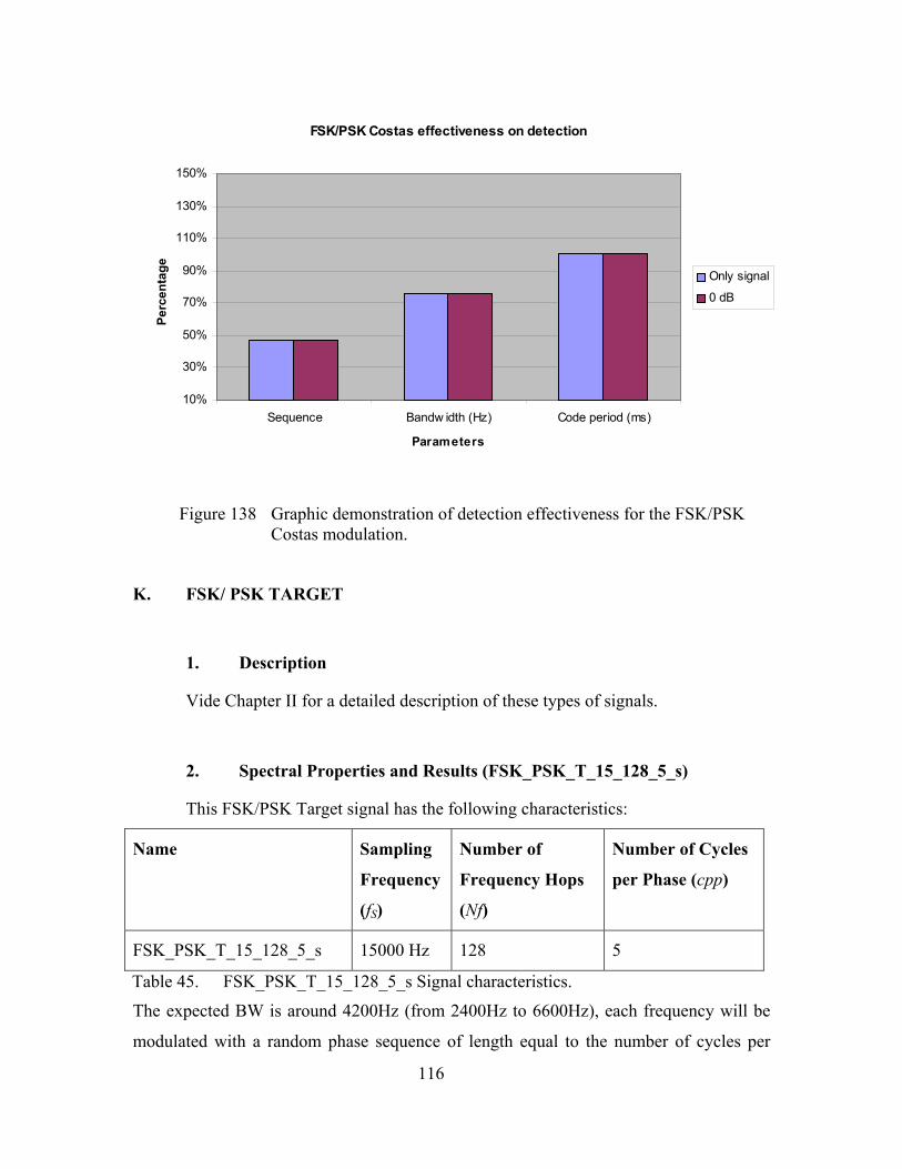
116
FSK/PSK Costas effectiveness on detection
10%
30%
50%
70%
90%
110%
130%
150%
Sequence Bandw idth (Hz) Code period (ms)
Parameters
Perc
enta
ge Only signal
0 dB
Figure 138 Graphic demonstration of detection effectiveness for the FSK/PSK Costas modulation.
K. FSK/ PSK TARGET
1. Description
Vide Chapter II for a detailed description of these types of signals.
2. Spectral Properties and Results (FSK_PSK_T_15_128_5_s)
This FSK/PSK Target signal has the following characteristics:
Name Sampling
Frequency
(fS)
Number of
Frequency Hops
(Nf)
Number of Cycles
per Phase (cpp)
FSK_PSK_T_15_128_5_s 15000 Hz 128 5
Table 45. FSK_PSK_T_15_128_5_s Signal characteristics.
The expected BW is around 4200Hz (from 2400Hz to 6600Hz), each frequency will be
modulated with a random phase sequence of length equal to the number of cycles per

117
phase. The following Figures reveal the frequency content of the signal (Figure 139), the
phase plots (Figure 140), the histogram of the frequency hops (Figure 141) and the
Estimated SCD (Figure 142, with N = 1024, frequency resolution of 16 Hz and M = 2) of
the signal analyzed.
Figure 139 PSD for a FSK/PSK Target signal (4200Hz BW, random phase with
length 5 and 5 cpp, only signal).
Figure 140 Random phase sequence of length 5 used inside each hop.
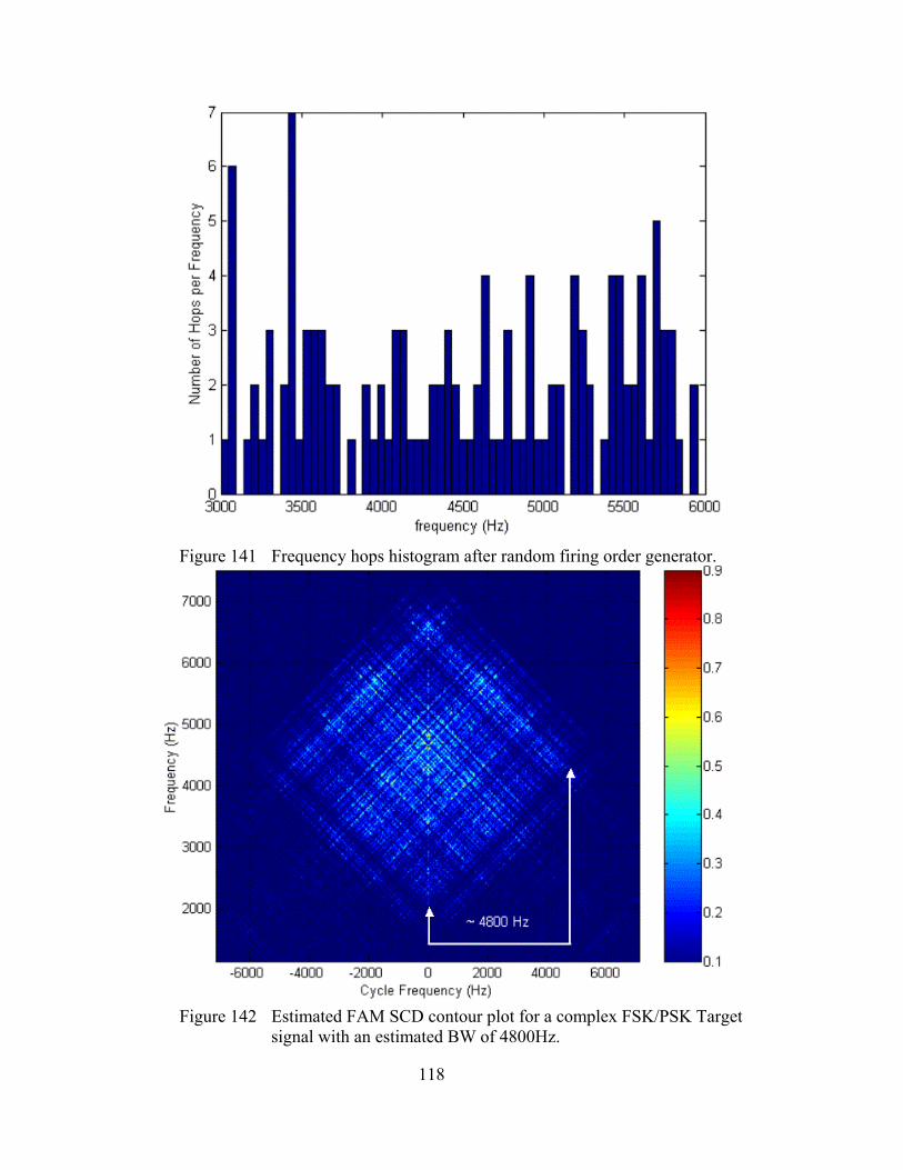
118
Figure 141 Frequency hops histogram after random firing order generator.
Figure 142 Estimated FAM SCD contour plot for a complex FSK/PSK Target
signal with an estimated BW of 4800Hz.

119
The given and measured features are summarized in the table below.
Feature Extraction
Characteristic Original Measured
Total BW for Entire Frequency Hopping Sequence 4200Hz 4800Hz Table 46. Comparison between measured and original characteristics for a FSK/PSK
Target signal.
The highest peaks of the spectrum of this signal (as seen in the PSD plot) may also be
detected in the bi-frequency plane. The firing order of the frequency hopping sequence
cannot be measured because we don’t have the time information in the output of the
cyclostationary processing.
This signal presented the highest degree of complexity of the whole set of signals
analyzed. The cause of this high complexity may be linked to the presence of two
pseudo-random factors:
• The frequency firing order; and
• The phase modulation for each frequency hop.
Since the emitter knows the pseudo-random sequence used, it can coherently demodulate
the signal with little effort but for a non-cooperative receiver this task becomes less
feasible. Table 48 shows a summary of all measurements for the FSK/PSK Target
modulation.
Sequence Bandwidth Code Period SNR 0 4800 0 Only signal 0 3000 0 Only signal 0 4200 0 Only signal 0 3000 0 Only signal
Table 47. Summary of all measurements for the FSK/PSK Target modulation.
Table 49 and graphics on Figure 143 show the detection effectiveness of the
cyclostationary processing for the FSK/PSK Target case, comparing with the original
values. The analysis was performed for the only signal case, since the results from the
added White Gaussian Noise cases were all inconclusive.

120
FSK/PSK Target Detection Effectiveness
SequenceBandwidth (Hz)
Code period (ms)
Only signal 0% 95% 0% Table 48. Detection effectiveness for the FSK/PSK Target modulation.
FSK/PSK Target effectiveness on detection
10%
30%
50%
70%
90%
110%
130%
150%
Sequence Bandw idth (Hz) Code period (ms)
Parameters
Perc
enta
ge Only signal
0 dB
Figure 143 Graphic demonstration of detection effectiveness for the FSK/PSK Target modulation.
L. COMPARISON BETWEEN POLYPHASE CODES
The following figures show a comparison between Frank (Figure 144), P1 (Figure
145), P2 (Figure 146), P3 (Figure 147) and P4 (Figure 148), with the same number of
phases (Np2 or Np = 16), same carrier frequency (1kHz) and same number of carrier
cycles per phase (cpp=1), It is possible to see that there’s some difference between the
SCD estimated results for the various modulations. The general shape of Frank, P3 and
P4 are very similar but P1 and P2 stand out very easily from the group. The absence of
time in the plots prevents us to see the phase changes along the code. The number of
phases may be calculated, as seen on the previous sections, by measuring the carrier
frequency, the bandwidth and the code period. Both cyclostationary algorithms were very
effective on determining all parameters for the LPI Radar signals with larger bandwidth
(cpp=1) and shorter code periods.

121
Figure 144 Estimated DFSM SCD contour plot for a Frank signal with 1150Hz
carrier, BW of 1000 Hz, Np2=16 and cpp=1.
Figure 145 Estimated DFSM SCD contour plot for a P1 signal with 900Hz
carrier, BW of 1000 Hz, Np2=16 and cpp=1.

122
Figure 146 Estimated DFSM SCD contour plot for a P2 signal with 1050Hz
carrier, BW of 950 Hz, Np2=16 and cpp=1.
Figure 147 Estimated DFSM SCD contour plot for a P3 signal with 1150Hz
carrier, BW of 1000 Hz, Np=16 and cpp=1.
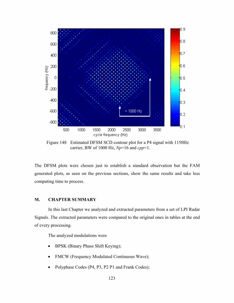
123
Figure 148 Estimated DFSM SCD contour plot for a P4 signal with 1150Hz
carrier, BW of 1000 Hz, Np=16 and cpp=1.
The DFSM plots were chosen just to establish a standard observation but the FAM
generated plots, as seen on the previous sections, show the same results and take less
computing time to process.
M. CHAPTER SUMMARY
In this last Chapter we analyzed and extracted parameters from a set of LPI Radar
Signals. The extracted parameters were compared to the original ones in tables at the end
of every processing.
The analyzed modulations were
• BPSK (Binary Phase Shift Keying);
• FMCW (Frequency Modulated Continuous Wave);
• Polyphase Codes (P4, P3, P2 P1 and Frank Codes);

124
• Costas Codes (Frequency Hopping);
• FSK/PSK (Combined Frequency Shift Keying and Phase Shift Keying) with a
Costas frequency distribution; and
• FSK/PSK (Combined Frequency Shift Keying and Phase Shift Keying) with a
target matched frequency distribution
It was possible to see that both time and frequency-smoothing methods of
cyclostationary processing may be applied to analyze these types of signals yielding
fairly appropriate results for the majority of the signals. A comparison between the
polyphase codes is also presented.

125
V. CONCLUSIONS AND RECOMMENDATIONS
This thesis effort was developed in order to implement two cyclostationary
processing techniques (Time and Frequency-Smoothing algorithms). The Time
Smoothing FFT Accumulation Method and the Direct Frequency Smoothing Method
were implemented in MATLAB® Version 6.1 [4] and tested in simulations using a
standardized data set. During this work it was possible to verify that the cyclostationary
processing approach is very suitable for analyzing radar signals with LPI characteristics.
Depending on the type of modulation, the processing and feature extraction can be more
or less difficult. The analysis of LPI signals can be improved for any type of signals with
the combination of the algorithms implemented here and other techniques such as:
• Parallel Filter Arrays and Higher Order Statistics [5];
• Quadrature Mirror Filtering [6]; and
• Wigner-Ville Distribution [7].
The similarities between the DFSM results and the FAM results go until a certain
level; in the zoomed plots we see that the channel pair regions are a little different in
shape and size, although they occur in the same values for frequency and cycle
frequency. This may be the result of the different windows applied in each method
(Hamming window for FAM and square window for DFSM). The computing time is also
noticeable larger, two or three times more, for the DFSM routine in comparison to the
FAM routine. The FAM implementation is recommended for long signals with a large
number of samples.
Both methods were very effective for phase modulated signals (BPSK, Frank, P1,
P2, P3, P4 and FSK/PSK Costas) and for FH signals (Costas) until signal-to-noise ratios
of 0dB and –6dB. The FMCW results showed more variation and errors in the results,
comparing to the original characteristics of the signals, even on the signal-only cases. The
FSK/PSK Target signal was also very difficult to analyze but mainly due to its pseudo-
random characteristic and complexity. In the technical report [10], signals with different
bandwidths and different code rates were included. It is possible to see that the
126
cyclostationary methods are very effective for signals with larger bandwidth and larger
code rates. In order to improve the computation time, a parallel processing
implementation is recommended for future work, using clusters or PC-based parallel
processors for academic purposes.
Starting from the extracted features, we recommend a future research on the
automatic classification of these types of signals as a form of maintaining the continuity
of this work. Neural networks have being exhaustively pointed as a viable solution for
accomplishing this task. The use of MATLAB® Version 6.1 and GUIDE Version 2.0 [4]
was very important to the success of this research and helped the development of a very
useful tool for future academic applications in Electronic Warfare and Signal Processing
oriented courses of the Naval Post Graduate School.

127
APPENDIX A. CYCLOSTATIONARY IMPLEMENTATION CODES (CYCLO.M, FAM.M AND DFSM.M)
%%%%%%%%%%%%%%%%%%%%%%%%%%%%%%%%%%%%%%%%%%%%%%%%%%% % % CYCLO.M % % Use: GUI implementation for inputing parameters in Cyclostationary Signal Processing Methods: DFSM.m and FAM.m % % Inputs: Path of the file to be analyzed; Name of the file; Sampling Frequency used in the generation of the file to be analyzed, % desired frequency resolution and desired method to be used (DFSM or FAM) % % Output: Various different plots exploring the bi-frequency plane representation typical of cyclostationary processing % % Created by Antonio F. Lima, Jr.-1o Ten. Av. Brazilian Air Force - March/2002 %%%%%%%%%%%%%%%%%%%%%%%%%%%%%%%%%%%%%%%%%%%%%%% % These are default commands and comments from the MATLAB® GUI guide tool % DO NOT EDIT !! %%%%%%%%%%%%%%%%%%%%%%%%%%%%%%%%%%%%%%%%%%%%%%% function varargout = cyclo(varargin) % CYCLO Application M-file for cyclo.fig % FIG = CYCLO launch cyclo GUI. % CYCLO('callback_name', ...) invoke the named callback. % Last Modified by GUIDE v2.0 01-May-2002 12:56:05 if nargin == 0 % LAUNCH GUI fig = openfig(mfilename,'reuse'); % Use system color scheme for figure: set(fig,'Color',get(0,'defaultUicontrolBackgroundColor')); % Generate a structure of handles to pass to callbacks, and store it. handles = guihandles(fig); guidata(fig, handles); if nargout > 0 varargout{1} = fig; end elseif ischar(varargin{1}) % INVOKE NAMED SUBFUNCTION OR CALLBACK try if (nargout) [varargout{1:nargout}] = feval(varargin{:}); % FEVAL switchyard else feval(varargin{:}); % FEVAL switchyard end catch

128
disp(lasterr); end end %% %%%%%%%%%%%%%% %%%%%%%%%%%% %%%%%%%%%%%% %%%%%%%%%% % These are the GUI functions definitions and global variables % -------------------------------------------------------------------- function varargout = edit3_Callback(h, eventdata, handles, varargin) d = get(h,'String'); handles.edit3 = d; % Save file path in global variable handles.edit3 (path = handles.edit3) guidata(h,handles); % -------------------------------------------------------------------- function varargout = edit1_Callback(h, eventdata, handles, varargin) name = get(h,'String'); handles.edit1 = name; % Save file name in global variable handles.edit1 (filename = handles.edit1) if isstr(name) else errordlg('Filename: Please enter a valid file name (B_1_7_7_s is default)', 'Bad input', 'modal') end guidata(h,handles); % -------------------------------------------------------------------- function varargout = edit2_Callback(h, eventdata, handles, varargin) fs = str2double(get(h,'String')); handles.edit2 = fs;% Save sampling frequency in global variable handles.edit2 (fs = handles.edit2) if isnan(fs) errordlg('Sampling Frequency: Please enter a numeric value (Hz)', 'Bad input', 'modal') end guidata(h,handles); % -------------------------------------------------------------------- function varargout = popupmenu1_Callback(h, eventdata, handles, varargin) val = get(h,'Value'); switch val % Switches between the values chosen by user on popupmenu case 1 handles.popupmenu1 = 128;% Save frequency resolution in global variable handles.popupmenu3 (df = handles.popupmenu3) case 2 handles.popupmenu1 = 64;% Save frequency resolution in global variable handles.popupmenu3 (df = handles.popupmenu3) case 3 handles.popupmenu1 = 32;% Save frequency resolution in global variable handles.popupmenu3 (df = handles.popupmenu3)

129
case 4 handles.popupmenu1 = 16;% Save frequency resolution in global variable handles.popupmenu3 (df = handles.popupmenu3) case 5 handles.popupmenu1 = 8;% Save frequency resolution in global variable handles.popupmenu3 (df = handles.popupmenu3) % case 6 handles.popupmenu1 = 4;% Save frequency resolution in global variable handles.popupmenu3 (df = handles.popupmenu3) case 7 handles.popupmenu1 = 2;% Save frequency resolution in global variable handles.popupmenu3 (df = handles.popupmenu3) end % More options may be added following the same pattern. guidata(h,handles); % -------------------------------------------------------------------- function varargout = popupmenu2_Callback(h, eventdata, handles, varargin) Mval = get(h,'Value'); switch Mval % Switches between the values chosen by user on popupmenu case 1 handles.popupmenu2 = 2;% Save reliability condition M in global variable handles.popupmenu2 (M = handles.popupmenu2) case 2 handles.popupmenu2 = 4;% Save reliability condition M in global variable handles.popupmenu2 (M = handles.popupmenu2) case 3 handles.popupmenu2 = 8;% Save reliability condition M in global variable handles.popupmenu2 (M = handles.popupmenu2) end guidata(h,handles); % % -------------------------------------------------------------------- function varargout = togglebutton1_Callback(h, eventdata, handles, varargin) dfsm;% Runs frequency smoothing method (DFSM.m), using the values entered - Direct Frequency Smoothing Method % -------------------------------------------------------------------- function varargout = togglebutton2_Callback(h, eventdata, handles, varargin) fam;% Runs time smoothing method (FFTAM.m), using the values entered - FFT Accumulation Method
130
%%%%%%%%%%%%%%%%%%%%%%%%%%%%%%%%%%%%%%%%%%%%%%% % FAM.M % Cyclostationary Estimator using the time smoothing FFT Accumulation Algorithm. % Part of the LPI oriented thesis work with Prof. P.E. PACE and Prof. H. LOOMIS % Student: Antonio F. LIMA Jr. - 1st. Lt. Brazilian Air Force %%%%%%%%%%%%%%%%%%%%%%%%%%%%%%%%%%%%%%%%%%%%%%% % Getting input data from the global variables generated by GUI cyclo_s.m and calculating constants % present_directory = cd; % Save present directory to a variable to make the GUI go back to it in the end path = handles.edit3; % Saving the path information in a variable cd (path);% Loading the file from the specified path filename = handles.edit1; % File to be analyzed from GUI generated global variable handles.edit1 fs = handles.edit2; % Sampling frequency from GUI generated global variable handles.edit2 df = handles.popupmenu1; % Frequency Resolution from GUI generated global variable handles.popupmenu3 M = 2; % df/dalpha = M >> 1 (reliability condition) dalpha = df/M; load (filename); %loading file to be analyzed in workspace x = I+ j.*Q;% using complex signal (for Real part only, use only I – input data file needs to be formatted as
% described in (4) % Defining parameters Np = pow2(nextpow2(fs/df)); % Initially, it is the number of rows in the channelization matrix (X) or % the number of input channels defined by fs/df L = Np/4; % Overlap factor in order to reduce the number of short time fft's % L is the offset between points in the same column at consecutive rows % should be less than or equal to Np/4 (Prof. Loomis paper) P = pow2(nextpow2(fs/dalpha/L)); % Number of columns formed in the channelization matrix (X) N = P*L; % Total number of points in the input data to be processed %%%%%%%%%%%%%%%%%%%%%%%%%%%%%%%%%%%%%%%%%%%%%%%%%%%% % Input channelization - this part limits the input total number of points to be analyzed. It also generates a Np X P matrix % (X) with shifted versions of the input vector in each column. if length(x)<N x(N) = 0; elseif length (x)>N x = x(1:N); end NN = (P-1)*L+Np; xx = x; xx(NN) = 0; xx = xx(:); X = zeros(Np,P);
131
for k = 0:P-1 X(:,k+1) = xx(k*L+1:k*L+Np); % X = (Np X P) Channelization input matrix end %%%%%%%%%%%%%%%%%%%%%%%%%%%%%%%%%%%%%%%%%%%%%%%%%%% % Windowing (Hamming window) - a vector of length Np is created with the MATLAB® 'hamming' function, then this vector is % inserted in a Np X Np matrix diagonal and this result is multiplied by the channelized input matrix (X). a = hamming (Np); XW = diag(a)*X; %%%%%%%%%%%%%%%%%%%%%%%%%%%%%%%%%%%%%%%%%%%%%%%%%%% % First FFT - this is the first short time fft (Np points long) applied to each column of matrix X. XF1 = fft(XW); XF1 = fftshift(XF1); XF1 = [XF1(:,P/2+1:P) XF1(:,1:P/2)]; %%%%%%%%%%%%%%%%%%%%%%%%%%%%%%%%%%%%%%%%%%%%%%%%%%% %Downconversion - the short sliding fft's results are shifted to base band to obtain decimated complex demodulate sequences [2] E = zeros(Np,P); for k = -Np/2:Np/2-1 for m = 0:P-1 E(k+Np/2+1, m+1) = exp(-i*2*pi*k*m*L/Np); end end XD = XF1.*E; XD = conj(XD'); % Transposing the matrix and taking the complex conjugate of the signal clear ('XF1', 'E', 'XW', 'X', 'x','I', 'Q'); % cleaning up memory space %%%%%%%%%%%%%%%%%%%%%%%%%%%%%%%%%%%%%%%%%%%%%%%%%%% % Multiplication - the product sequences between each one of the complex demodulates and the complex conjugate of the others % are formed. This forms the area in the bi-frequency plane as explained in [2] figures 4 , 7 and 10 XM = zeros(P,Np^2); for k = 1:Np for c = 1:Np XM(:,(k-1)*Np+c) = (XD(:,k).*conj(XD(:,c))); end end %%%%%%%%%%%%%%%%%%%%%%%%%%%%%%%%%%%%%%%%%%%%%%%%%%%% Second FFT - a P point FFT is applied to XM (in each of its columns) XF2 = fft(XM); XF2 = fftshift(XF2); XF2 = [XF2(:,Np^2/2+1:Np^2) XF2(:,1:Np^2/2)]; XF2 = XF2 (P/4:3*P/4,:); MM = abs(XF2); %%%%%%%%%%%%%%%%%%%%%%%%%%%%%%%%%%%%%%%%%%%%%%%%%%%
132
%Output matrices range alpha0 = -fs:fs/N:fs; f0 = -fs/2:fs/Np:fs/2; Sx = zeros(Np+1, 2*N+1); %%%%%%%%%%%%%%%%%%%%%%%%%%%%%%%%%%%%%%%%%%%%%%%%%%% % Display only the data inside the range of interest - centralizes the bi-frequency plane according to alpha0 and f0 vectors for k1 = 1:P/2+1 for k2 = 1:Np^2 if rem(k2,Np) == 0 c = Np/2 - 1; else c = rem(k2,Np) - Np/2 - 1; end k = ceil(k2/Np)-Np/2-1; p = k1-P/4-1; alpha = (k-c)/Np+(p-1)/N; f = (k+c)/2/Np; if alpha<-1 | alpha>1 k2 = k2+1; elseif f<-.5 | f>.5 k2 = k2+1; else kk = 1+Np*(f + .5); ll = 1+N*(alpha + 1); Sx(round(kk), round(ll)) = MM(k1,k2); end end end clear ('alpha', 'XM', 'XF2', 'MM', 'f'); % cleaning up memory space Sx = Sx./max(max(Sx)); % Normalizes the magnitudes of the values in output matrix (maximum = 1) %%%%%%%%%%%%%%%%%%%%%%%%%%%%%%%%%%%%%%%%%%%%%%%%%%%% % Plotting Routines % saves file containing results % savefile = 'FFTAM_result_s'; % save(savefile,'filename','N','alpha0', 'f0', 'Sx', 'M', 'df') % clear all; % clc; % % load ('FFTAM_result_s.mat'); % figure (df + M); % mesh % view (-55,70); % xlabel ('cycle frequency'); ylabel('frequency'); zlabel ('SCD magnitude'); % title (['Time Smoothing (FFTAM) generated SCD for ', filename, ', df = ', int2str(df), ' and N = ', int2str(N)]); % % % figure % % mesh (alpha0,f0, Sx, 'EdgeColor', 'interp');

133
% % view (0,90); % % xlabel ('cycle frequency'); ylabel('frequency'); zlabel ('SCD magnitude'); % % title (['SCD for ', filename, ' N=', int2str(N)]); % % % % figure % subplot(2,2,1:2); % plot (f0, Sx); grid; % title (['Time Smoothing Processing for ', filename, ', df = ', int2str(df), ' and N = ', int2str(N)]); % xlabel ('frequency (Hz)'); ylabel('SCD magnitude'); % subplot(2,2,3:4); % plot (alpha0, Sx); grid; % xlabel ('cycle frequency (Hz)'); ylabel ('SCD magnitude'); % % figure % % subplot(2,2,1:2); % % contour (alpha0, f0, Sx); grid; % % xlabel('cycle frequency (Hz)'); ylabel('frequency (Hz)'); % % title (['Time Smoothing (FFTAM) generated SCD for ', filename, ', df = ', int2str(df), ' and N = ', int2str(N)]); % % zoom(2);colorbar; % % subplot(2,2,3:4); % % contour (alpha0, f0, Sx); grid; % % xlabel('cycle frequency (Hz)'); ylabel('frequency (Hz)'); % % zoom(2);colorbar; % figure contour (alpha0, f0, Sx); grid; xlabel('cycle frequency (Hz)'); ylabel('frequency (Hz)'); title (['Time Smoothing (FFTAM) generated SCD for ', filename, ', df = ', int2str(df), ' and N = ', int2str(N)]); colorbar; delete ('FFTAM_result_s.mat'); % newname = ['FFTAM_' filename]; % cd('C:\Documents and Settings\aflima\Tese\Result Figures'); % saveas (gcf, newname, 'jpg'); cd('C:\Documents and Settings\aflima\Tese\cyclo');

134
%%%%%%%%%%%%%%%%%%%%%%%%%%%%%%%%%%%%%%%%%%%%%%%%%%% % *** Cyclostationary Estimator using the Direct Frequency Smoothing Method algorithm.*** % Part of the LPI oriented thesis work with Prof. P.E. PACE and Prof. H. LOOMIS % Student: Antonio F. LIMA Jr. - 1st. Lt. Brazilian Air Force %%%%%%%%%%%%%%%%%%%%%%%%%%%%%%%%%%%%%%%%%%%%%%%%%%% % Getting input data from the global variables generated by GUI cyclo_s.m % function f = dfsm_s (x); % present_directory = cd; % Save present directory to a variable to make the GUI go back to it in the end path = handles.edit3; % Saving the path information in a variable cd (path);% Loading the file from the specified path filename = handles.edit1; % File to be analyzed Fs = handles.edit2; % Sampling frequency df = handles.popupmenu1; % Frequency Resolution M = 2; % Smoothing window range load (filename); x = I;% Using real part of signal N = (M*Fs)/df; N = pow2 (nextpow2(N)); % windowing record for FFT X = fft(x,N); % fft of the truncated (or zero padded) time series X = fftshift(X);% shift components of fft Xc = conj(X); % precompute the complex conjugate vector S = zeros (N,N); % size of the Spectral Correlation Density matrix f = zeros (N,N); % size of the frequency matrix; alfa = zeros (N,N); % size of the cycle frequency matrix F = Fs/(2*N); % precompute constants - F = Fs/(2*N); G = Fs/N; % precompute constants - G = Fs/N; m = -M/2+1:M/2; % set frequency smoothing window index for k = 1:N % fix k % computes vectors of f and alfa, % store frequency and cycle frequency data for given k. k1 = 1:N; f(k,k1) = F*(k+k1-1) - Fs/2; % Computes f values and shift them to center in zero (f = (K+L)/2N) [1] alfa(k,k1) = G*(k-k1 + N-1) - Fs; % Computes alfa values and shift them to center in zero (alfa = (K-L)/N) [1] for k1 = 1:N %fix k1 = J %calculate X(K+m) & conj (X(J+m)) for arguments of X(1:N) only B = max(1-k, 1-k1); % Largest min of 1 <= (K+m)| (J+m) <= N A = min (N-k, N-k1); % Smallest max of 1 <= (K+m)| (J+m) <= N n = m((m<=A) & (m>=B)); %fix the index out of range problem by % truncating the window if isempty(n) S(k,k1) = 0; else p = k+n; q = k1+n; Y = X(p).*Xc(q);

135
S(k,k1) = sum(Y); end end end S = abs(S./max(max(S)));% normalize output matrix %%%%%%%%%%%%%%%%%%%%%%%%%%%%%%%%%%%%%%%%%%%%%%%%%%% % Saving variables, cleaning up memory and running plots savefile = 'DFSM_result_s'; %save(savefile,'I', 'Q', 'alfa', 'f', 'S', 'N', 'Fs', 'filename', 'M', 'df') save(savefile,'alfa', 'f', 'S', 'N','filename', 'M', 'df') clear all; load ('DFSM_result_s.mat'); % figure (2*(df+M)); % mesh (alfa,f, S, 'EdgeColor', 'interp'); % view (-55,70); % xlabel ('cycle frequency'); ylabel('frequency'); zlabel ('SCD magnitude'); % title (['Frequency Smoothing (DFSM) generated SCD for ', filename, ' df = ', int2str(df), ' N = ', int2str(N)]); % % % figure (2*(df+M) + 1); % mesh (alfa,f, S, 'EdgeColor', 'interp'); % view (0,90); % xlabel ('cycle frequency'); ylabel('frequency'); zlabel ('SCD magnitude'); % title (['SCD for', filename, ' df =', int2str(df), ' N=', int2str(N)]); % % figure(2*(df+M) + 2) % % subplot (2,2,1:2) % psd(I, N, Fs); % title(['I - real part for nfft = ', int2str(N), ' and for default nfft = 256']); % subplot (2,2,3:4) % psd(I, [], Fs); % subplot (2,2,3) % psd(I+j.*Q, N/2, Fs); % title('I+j.Q - complex'); % subplot (2,2,4) % psd(I-j.*Q, N/2, Fs); % title('I-j.Q - complex'); % % % figure % subplot(2,2,1:2); % plot (f, S); grid; % title (['Frequency Smoothing Processing for ', filename, ', df = ', int2str(df), ' and N = ', int2str(N)]); % xlabel ('frequency (Hz)'); ylabel('SCD magnitude'); % subplot(2,2,3:4); % plot (alfa, S); grid; % xlabel ('cycle frequency (Hz)'); ylabel ('SCD magnitude'); % % % % figure (2*(df+M) + 5) % subplot(2,2,1:2); % contour (alfa, f, S); grid; % xlabel('cycle frequency (Hz)'); ylabel('frequency (Hz)');

136
% title (['Frequency Smoothing (DFSM) generated SCD for ', filename, ', df = ', int2str(df), ' and N = ', int2str(N)]); % zoom(2);colorbar; % subplot(2,2,3:4); % contour (alfa, f, S); grid; % xlabel('cycle frequency (Hz)'); ylabel('frequency (Hz)'); % zoom(2);colorbar; figure contour (alfa, f, S); grid; xlabel('cycle frequency (Hz)'); ylabel('frequency (Hz)'); title (['Frequency Smoothing (DFSM) generated SCD for ', filename, ', df = ', int2str(df), ' and N = ', int2str(N)]); colorbar; delete ('DFSM_result_s.mat'); newname = ['DFSM_' filename]; cd('C:\Documents and Settings\aflima\Tese\Result Figures'); saveas (gcf, newname, 'jpg'); cd('C:\Documents and Settings\aflima\Tese\cyclo');
137
APPENDIX B. FSK/PSK GENERATION CODES
% FREQUENCY AND PHASE SHIFT COMBINED CODE using Costas Frequency modulation % Developed by Antonio Lima and Harsha Tummala % July, 2002 % Phase code for FSK/PSK from IEEE International Radar Conference Paper - 1990 % “The ambiguity properties of FSK/PSK signals” % by J. Patrick Donohoe, and Franklin M. Ingels clear all; clc; disp('********************************************************************************'); disp('FREQUENCY AND PHASE SHIFT CODE (FSK/PSK) USING COSTAS FREQUENCIES******'); disp('********************************************************************************'); % DEFAULT VARIABLES A=1; % Amplitude of CW fs =15e3; % Sample Rate SNR_dB = 0; %Signal to Noise Ratio cpf=1; %Cycles per frequency (> 10) scale=5; % Scaling for plotting time domain graphs barker = 5; % Number of Barker Bots for phase modulation j=sqrt(-1); % j % NEW INPUT newvar = 1; while newvar == 1; disp(' ') disp('WHICH PARAMETER DO YOU WANT TO SET ? ') disp(' ') fprintf('1. Amplitude of frequencies - A= %g.\n', A) fprintf('2. Sampling frequency - fs (Hz)= %g.\n', fs) fprintf('3. Signal to noise ratio - SNR_dB (dB) = %g.\n', SNR_dB) fprintf('4. Cycles per frequency = %g.\n', cpf) fprintf('5. Number of bits per Barker code for phase modulation - barker (13/11/7/5)= %g.\n', barker) fprintf('6. No changes\n') disp(' ') option= input('Select a option: '); switch option case 1 A=input('New amplitude of the carrier signal= '); case 2 fs=input('New sampling frequency (Hz)= '); case 3 SNR_dB=input('New signal to noise ratio (dB)= '); case 4 cpf=input('New number of cycles per frequency = '); case 5 barker=input('New number of bits for Barker Code = '); case 6 newvar = 0; end

138
clc; end % FREQUENCY CHOICES newvar = 1; while newvar == 1; disp(' ') disp('WHICH COSTAS FREQUENCY SEQUENCE WOULD YOU LIKE TO USE ? ') disp(' ') disp('1. 4, 7, 1, 6, 5, 2, 3 '); disp('2. 2, 6, 3, 8, 7, 5, 1 '); disp('3. 4, 1, 6, 7, 5, 3, 2 '); disp('4. 5, 6, 8, 2, 4, 3, 1 '); disp('5. 4, 9, 2, 5, 1, 9, 8 '); disp('6. 2, 4, 1, 1, 7, 11, 9'); disp('7. 2, 2, 5, 1, 3, 7, 4 '); disp(' ') option2= input('Select an option: '); freq=[4 7 1 6 5 2 3; 2 6 3 8 7 5 1; 4 1 6 7 5 3 2; 5 6 8 2 4 3 1; 4 9 2 5 1 9 8; 2 4 1 1 7 11 9; 2 2 5 1 3 7 4]*1000 switch option2 case 1 seq=freq(1,:); case 2 seq=freq(2,:); case 3 seq=freq(3,:); case 4 seq=freq(4,:); case 5 seq=freq(5,:); case 6 seq=freq(6,:); case 7 seq=freq(7,:); end newvar=0; clc; end % Create spanning Barker frequency

139
minimum=min(seq); SAR=ceil(fs/minimum); % Sampling ratio tb=1/(fs); % Sampling period % This section generates I & Q without COSTAS phase shift and I & Q with Phase shift. The signals are
generated % five times by the outer loop. The variable 'index' is used to generate a time vector for time domain plots. % The signal is generated at seven samples per phase change. pw = 1; if barker==13 phase = [ones(1,pw*5),-(ones(1,pw*2)),ones(1,pw*2),-ones(1,pw),ones(1,pw),-
ones(1,pw),ones(1,pw)];% 13 bits elseif barker==11 phase = [ones(1,pw*3),-(ones(1,pw*3)),ones(1,pw),-ones(1,pw),-ones(1,pw),ones(1,pw),-ones(1,pw)];%
11 bits elseif barker==7 phase = [ones(1,pw*3),-(ones(1,pw*2)),ones(1,pw),-ones(1,pw)];% 7 bits elseif barker==5 phase = [ones(1,pw*3),-(ones(1,pw)),ones(1,pw)];% 5 bits end index=0; for pp = 1:5 for xx=1:7 for nn = 1:barker for n=1:SAR*cpf IWO(index+1)=A*cos(2*pi*seq(xx)*(n-1)*tb); QWO(index+1)=A*sin(2*pi*seq(xx)*(n-1)*tb); I(index+1)=A*cos(2*pi*seq(xx)*(n-1)*tb)*phase(nn); Q(index+1)=A*sin(2*pi*seq(xx)*(n-1)*tb)*phase(nn); time(index+1)=index*tb; %time vector cumulation index = index +1; end end end end %Power Spectral Density for I with phase shift & with WGN with Signal to noise ratios (SNR) = [0,-
5,5,10,-10,-20]

140
%for loop makes calculations and plots for each value of SNR for WGN [a,b]=size(I); SNR=10^(SNR_dB/10); power=10*log10(A^2/(2*SNR));%calculate SNR in dB for WGN function noise=wgn(a,b,power);%calculate noise at specified SNR IN=I+noise; %add noise to I with FSK/PSK phase shift IPWON=I; %I with phase shift without noise QN=Q+noise; %add noise to Q with FSK/PSK phase shift QPWON=Q; %Q with phase shift without noise ffs = fs/1000; %******************************************************* %PLOTS %****************************************************** disp(' ') plt = input('Do you want to generate plots of the signal (Y/y or N/n) ?','s'); disp(' ') if (plt == 'Y') | (plt =='y') disp(' ') %Plot Power Spectral Density for I without phase shift % figure ; % open new figure for plot % psd(IWO,[],fs); %Power Spectral Density of I without Phase shift % title(['PSD of I without Phase Shift or Noise']); %Plot PSD of I+ FSK/PSK Phase + WGN and Time Domain of I + FSK/PSK Phase figure ;% open new figure for plot signal = I+j*Q; psd(signal,[],fs);%plot PSD for specified noise SNR title(['PSD of FSK-PSK-C-' num2str(option2) '-' num2str(ffs) '-' num2str(barker) '-' num2str(cpf) '-s
I+j*Q']); figure ;% open new figure for plot signal = IN+j*QN; psd(signal,[],fs);%plot PSD for specified noise SNR title(['PSD of FSK-PSK-C-' num2str(option2) '-' num2str(ffs) '-' num2str(barker) '-' num2str(cpf) '-'
num2str(SNR_dB) ' I+j*Q']); % %plot time domain signal I with FSK/PSK phase shift and WGN at specified SNR % figure ;%open new figure for plot % plot(time(1:floor(size(time,2)/scale)),I(1:floor(size(time,2)/scale))); % title(['FSK-PSK-C-' num2str(option2) '-' num2str(ffs) '-' num2str(barker) '-s Time Domain']); % xlabel('{\itTime - Seconds} '); % ylabel('Amplitude'); % grid on; % % Now check to see if signal is correct by plotting phase shift alone and then determining phase shift
from I+jQ. % To determine phase shift, look at the phase angle of I+jQ at every 7th time interval. Expect to see the
FSK/PSK phase % function plot repeated 5 times after unwrapping and detrending the phase angle. figure;%open new figure for plot plot(phase);

141
title(['FSK-PSK-C-' num2str(option2) '-' num2str(ffs) '-' num2str(barker) '-' num2str(cpf) '-s Phase Shift for each Costas frequency hop']);
xlabel('i - index for phase change'); ylabel('FSK/PSK Phase Shift - Theta'); grid on; else disp('Signal not plotted') fprintf('\n\n') end % This section generates the files for analysis INP=IN';%transpose I with noise and FSK/PSK phase shift for text file QNP=QN';%transpose Q with noise and FSK/PSK phase shift for text file IPWONT=IPWON';%transpose I with phase without noise for text file QPWONT=QPWON';%transpose Q with phase without noise for text file % % save results in data files I= INP(:,1); Q=QNP(:,1); II= IPWONT(:,1); QQ=QPWONT(:,1); disp(' ') saveresult = input('Do you want to save the new signal (Y/y or N/n) ?','s'); if (saveresult == 'Y') | (saveresult =='y') ffs=floor(fs/1e3); save(['FSK_PSK_C_' num2str(option2) '_' num2str(ffs) '_' num2str(barker) '_' num2str(cpf) '_'
num2str(SNR_dB)],'I','Q'); I=II; Q=QQ; save(['FSK_PSK_C_' num2str(option2) '_' num2str(ffs) '_' num2str(barker) '_' num2str(cpf) '_s'],'I','Q'); disp(' '); disp(['Signal and noise save as : FSK_PSK_C_' num2str(option2) '_' num2str(ffs) '_' num2str(barker) '_'
num2str(cpf) '_' num2str(SNR_dB)]); disp(['Signal only save as : FSK_PSK_C_' num2str(option2) '_' num2str(ffs) '_' num2str(barker) '_'
num2str(cpf) '_s']); disp(['Directory: ' num2str(cd)]); else disp(' ') disp('Signal not saved') fprintf('\n\n') end

142
% FREQUENCY AND PHASE SHIFT CODE (FSK/PSK) for a target frequency distribution % Developed by Antonio Lima and Harsha Tummala % July, 2002 % Phase code for FSK/PSK from IEEE International Radar Conference Paper % MATCHED FSK/PSK RADAR % by B. Jeffrey Skinner, J. Patrick Donohoe, and Franklin M. Ingels clear all; clc; disp('***********************************************************************'); disp('*************FREQUENCY AND PHASE SHIFT CODE (FSK/PSK)*************'); disp('***********************************************************************'); %DEFAULT VARIABLES A=1; % Amplitude of CW fs =15000; % Sampling Frequency SNR_dB = 0; % Signal to Noise Ratio scale=20; % Scaling for plotting time domain graphs j=sqrt(-1); % j global N; N=128; % Number of fsk/psk sections (frequency hops and phase changes) cpp = 5; % Number of cycles per phase % NEW INPUT newvar = 1; while newvar == 1; disp(' ') disp('WHICH PARAMETER DO YOU WANT TO SET ? ') disp(' ') fprintf('1. Amplitude of the carrier signal - A= %g.\n', A) fprintf('2. Sampling frequency - fs (Hz)= %g.\n', fs) fprintf('3. Signal to noise ratio - SNR_dB (dB) = %g.\n', SNR_dB) fprintf('4. Number of phase/frequency hops - N = %g.\n', N) fprintf('5. Number of cycles per phase - cpp = %g.\n', cpp) fprintf('6. No changes\n') disp(' ') option= input('Select a option: '); switch option case 1 A=input('New amplitude of the carrier signal= '); case 2 fs=input('New sampling frequency (Hz)= '); case 3 SNR_dB=input('New signal to noise ratio (dB)= '); case 4 N=input('New number of phase/frequency hops ='); case 5 cpp=input('New number of cycles per phase='); case 6 newvar = 0; end clc; end airplane; % Compute frequency hops values according to an airplane's frequency response
143
syn_test; % Generates frequency distribution according to previous probability distribution global target; % Compute Frequency, first call up airplane variable global detection; % tb=1/(fs); % Sampling period SAR=ceil(fs/min(detection)); % Sampling ratio (for smaller frequency) phase = rand(1,cpp); %Compute the phase encoding random sequence for each frequency burst greater = find(phase>=0.5); phase(greater) = pi; lesser = find(phase<0.5); phase(lesser) = 0; % This section generates I & Q without phase shift and I & Q with Phase shift. The signals are generated % five times the number of frequency hops by the outer loop. The variable 'index' is used to generate a
time vector for time domain plots. % The signal is generated at seven samples per phase change. index=0; % Time vector for time domain plots. for p=1:2% Generate the signal two times and store sequentially in corresponding vectors for ii = (1:N) %Loop for each frequency hop f = detection(ii,:); for kk = (1:size(target,1)) if f == target(kk,1) init_phase = target(kk,3); %defines initial phase of FSK sequence end end for n=1:SAR*cpp %Loop to increment time for single frequency value. I(index+1)=A*cos(2*pi*f*(n-1)*tb+phase(ceil(n/SAR))+init_phase); %Calculate in phase
component of signal with phase shift IWO(index+1)=A*cos(2*pi*f*(n-1)*tb); % Calculate in phase component of signal without phase
shift Q(index+1)=A*sin(2*pi*f*(n-1)*tb+phase(ceil(n/SAR))+init_phase); % Calculate quadrature
component of signal with phase shift QWO(index+1)=A*sin(2*pi*f*(n-1)*tb); %Calculate quadrature component of signal without
phase shift time(index+1)=index*tb; %time vector cumulation index = index +1; end end end %Power Spectral Density for I with phase shift & with WGN with Signal to noise ratios (SNR) = [0,-
5,5,10,-10,-20] %for loop makes calculations and plots for each value of SNR for WGN [a,b]=size(I); SNR=10^(SNR_dB/10); power=10*log10(A^2/(2*SNR));%calculate SNR in dB for WGN function noise=wgn(a,b,power);%calculate noise at specified SNR IN=I+noise; %add noise to I with FSK/PSK phase shift IPWON=I; %I with phase shift without noise QN=Q+noise; %add noise to Q with FSK/PSK phase shift
144
QPWON=Q; %Q with phase shift without noise ffs = fs/1000; %******************************************************* %PLOTS %****************************************************** disp(' ') plt = input('Do you want to generate plots of the signal (Y/y or N/n) ?','s'); disp(' ') if (plt == 'Y') | (plt =='y') disp(' ') global range; global airplane; %Plot Target Frequency Distribution and Range/Magnitude plot figure;% open new figure for plot plot(target(:,1), target(:,2)); title('Ship FFT ABS'); grid on title(['Original Target Frequency Probability Distribution']); xlabel('Frequency'); ylabel('Normalized Magnitude = Probability'); figure;% open new figure for plot plot(range, real(airplane(1:64))); title('Ship'); grid on title(['Original Target Range / Magnitude Plot']); xlabel('Range (ft)'); ylabel('Magnitude'); % Plot original frequency distribution histogram and frequency random firing distribution figure;% open new figure for plot orient tall; subplot(2,1,1), hist(detection(:,1),N); xlabel('Detection Index'); ylabel('Number of Occurences'); fid1=['Target SYNTHETIC']; title(fid1); subplot(2,1,2), bar(target(:,1), target(:,2)); xlabel('Detection Index') ylabel('Probability') fid2=['Target ORIGINAL']; title(fid2); %Plot Power Spectral Density for I without phase shift % figure ; % open new figure for plot % psd(IWO,[],fs); %Power Spectral Density of I without Phase shift % title(['PSD of I without Phase Shift or Noise']); %time domain plot of in phase signal I with phase shift % figure ; %open new figure for plot % % plot small portion of time domain signal I so that data will fit meaningfully in figure. % %floor(size(time,2)/scale) selects a small sample of the vectors to plot % plot (time(1:floor(size(time,2)/scale)),I(1:floor(size(time,2)/scale))); % title(['Time Domain of I with Phase Shift & no Noise']);
145
% xlabel('{\itTime - Seconds} '); % ylabel('Amplitude'); % grid on; % %Plot PSD of I+ FSK/PSK Phase + WGN and Time Domain of I + FSK/PSK Phase figure ;% open new figure for plot signal = I+j*Q; psd(signal,[],fs);%plot PSD for specified noise SNR title(['PSD of FSK-PSK-T-' num2str(ffs) '-' num2str(N) '-' num2str(cpp) '-s I+j*Q']); %plot time domain signal I with FSK/PSK phase shift and WGN at specified SNR figure ;%open new figure for plot plot(time(1:floor(size(time,2)/scale)),I(1:floor(size(time,2)/scale))); title(['FSK-PSK-T-' num2str(ffs) '-' num2str(N) '-' num2str(cpp) '-s Time Domain']); xlabel('{\itTime - Seconds} '); ylabel('Amplitude'); grid on; % Now check to see if signal is correct by plotting phase shift alone and then determining phase shift
from I+jQ. % To determine phase shift, look at the phase angle of I+jQ at every 7th time interval. Expect to see the
FSK/PSK phase % function plot repeated 5 times after unwrapping and detrending the phase angle. figure;%open new figure for plot plot(phase); title(['FSK-PSK-T-' num2str(ffs) '-' num2str(N) '-' num2str(cpp) '-s Phase Shift ']); xlabel('i - index for phase change'); ylabel('FSK/PSK Phase Shift - Theta'); grid on; else disp('Signal not plotted') fprintf('\n\n') end % This section generates the files for analysis INP=IN';%transpose I with noise and FSK/PSK phase shift for text file QNP=QN';%transpose Q with noise and FSK/PSK phase shift for text file IPWONT=IPWON';%transpose I with phase without noise for text file QPWONT=QPWON';%transpose Q with phase without noise for text file % % save results in data files I = INP(:,1); Q = QNP(:,1); II = IPWONT(:,1); QQ = QPWONT(:,1); disp(' ') saveresult = input('Do you want to save the new signal (Y/y or N/n) ?','s'); if (saveresult == 'Y') | (saveresult =='y') ffs=floor(fs/1e3);

146
save(['FSK_PSK_T_' num2str(ffs) '_' num2str(N) '_' num2str(cpp) '_' num2str(SNR_dB)],'I','Q', 'detection');
I=II; Q=QQ; save(['FSK_PSK_T_' num2str(ffs) '_' num2str(N) '_' num2str(cpp) '_s'],'I','Q','detection'); disp(' '); disp(['Signal and noise save as : FSK_PSK_T_' num2str(ffs) '_' num2str(N) '_' num2str(cpp) '_'
num2str(SNR_dB)]); disp(['Signal only save as : FSK_PSK_T_' num2str(ffs) '_' num2str(N) '_' num2str(cpp) '_s']); disp(['Directory: ' num2str(cd)]); else disp(' ') disp('Signal not saved') fprintf('\n\n') end %%%%%%%%%%%%%%%%%%%%%%%%%%%%%%%%%%%%%%%%%%%%%%%%%%% % This part may be implemented on a different file %%%%%%%%%%%%%%%%%%%%%%%%%%%%%%%%%%%%%%%%%%%%%%%%%%% function airplane = airplane; global target; global airplane; global range; % Target range Profile airplane = [complex(0,-0.00000032:0.00000001:-0.00000016), complex(-0.001,-0.00000015), complex(-
0.002,-0.00000014), complex(-0.003,-0.00000013), complex(-0.0027,-0.00000012), complex(-0.0025,-0.00000011), ...
complex(-0.0022,-0.00000010), complex(-0.0020, -0.00000009), complex(-0.0017, -0.00000008), complex(-0.0015,-0.00000007), complex(-0.0023, -0.00000006), complex(-0.003, -0.00000005), complex(-0.0015, -0.00000004), ...
complex(0,-0.00000003), complex(0,-0.00000002), complex(-0.0015, -0.00000001), complex(-0.003,0),complex(0.028, 0.00000001), complex(-0.0075, 0.00000002), complex(0.014, 0.00000003), complex(0.013,0.00000004), complex(-0.038,0.00000005), ...
complex(-0.003, 0.00000006), complex(-0.004, 0.00000007), complex(-0.005, 0.00000008), complex(-0.015, 0.00000009), complex(0.003, 0.0000001), complex(-0.0015, 0.00000011:0.00000001:0.00000016), complex(0, 0.00000017:0.00000001:0.00000031), complex(0,-0.00000032:0.00000001:0.00000031)];
% Target Time profile airplane_t = flipdim(airplane, 2); airplane_t = real(airplane_t).*(-1) + j.*(imag(airplane_t)); % FFT of the time record fo the target response airplane_1 = fft(airplane_t); airplane_2 = abs(fftshift(airplane_1)); ph_airplane = phase(airplane_1); freq_step = 64; % Number of frequency steps to be used fss = 12e6; fs = fss/2000; %Downsized sampling frequency (from 12MHz to 6000Hz) frequency = fs/2:fs/2/freq_step:fs - 1;
147
airplane_3 = airplane_2(64:127); total = sum(airplane_3); airplane_4 = airplane_3/total; target = [(frequency)', (airplane_4)', (ph_airplane(1:freq_step))']; range_bin = (fss*2e-9)^(-1); range = 1:range_bin:freq_step*range_bin-1; %%%%%%%%%%%%%%%%%%%%%%%%%%%%%%%%%%%%%%%%%%%%%%%%%%% % This part may be implemented on a different file %%%%%%%%%%%%%%%%%%%%%%%%%%%%%%%%%%%%%%%%%%%%%%%%%%% %% FREQUENCY SYNTHESIS ALGORITHM FOR FSK/PSK TARGET %% Frequencies are in the vector "detection" function syn_test = syn_test; fid=['Ship']; global N; global target; new_rec= target(:,1:2); %********************************************** %NO EDITS BELOW %********************************************** % PULL OFF THE DECIMAL DIGITS [nn,jo]=size(new_rec); % Determine number % of detections or rows % Pull off the density % decimal digits as strings “delta”=sprintf('%6.4f',new_rec(:,2)); ss=reshape(“delta”, 6, nn); ss=ss'; % Turn back into a number % with each digit a column “delta”s(:,[1])=str2num(ss(:,3)); “delta”s(:,[2])=str2num(ss(:,4)); “delta”s(:,[3])=str2num(ss(:,5)); “delta”s(:,[4])=str2num(ss(:,6)); %% kk =4; % NUMBER OF DECIMAL DIGITS % Define probabilities % p1 through p4 p0=0; p1=10^(-1) * sum(“delta”s(:,1)); p2=10^(-2) * sum(“delta”s(:,2)); p3=10^(-3) * sum(“delta”s(:,3)); p4=10^(-4) * sum(“delta”s(:,4)); % Determine pi values

148
pi0= 0; pi1= 10*p1; pi2= (10*p1)+(10^2 * p2); pi3= (10*p1)+(10^2 * p2)+(10^3 * p3); pi4= (10*p1)+(10^2 * p2)+(10^3 * p3) + (10^4 * p4); % Determine test values for % the uniform random variable ptest0=0; ptest1=p1; ptest2=ptest1+p2; ptest3=ptest2+p3; ptest4=ptest3+p4; % FILL MEMORY LOCATION % SET 1 ok=0; for j=1:nn % RANDOM VARIABLE INDEX if “delta”s(j,1)~=0 for i=1:”delta”s(j,1) mem(i+ok,1)=j; end ok=i+ok; end end if “delta”s(j,1)~=0 [mem_size xx]=size(mem); else mem_size = 0; xx = 0; end % FILL MEMORY LOCATIONS % SET 2 ok=0; for j=1:nn % RANDOM VARIABLE INDEX if “delta”s(j,2)~=0 for i=1:”delta”s(j,2) mem(i+ok+mem_size,1)=j; end ok=i+ok; end end [mem_size xx]=size(mem); % FILL MEMORY LOCATIONS % SET 3 ok=0; for j=1:nn % RANDOM VARIABLE INDEX if “delta”s(j,3)~=0 for i=1:”delta”s(j,3) mem(i+ok+mem_size,1)=j; end ok=i+ok;

149
end end [mem_size xx]=size(mem); % FILL MEMORY LOCATIONS % SET 4 ok=0; for j=1:nn % RANDOM VARIABLE INDEX if “delta”s(j,4)~=0 for i=1:”delta”s(j,4) mem(i+ok+mem_size,1)=j; end ok=i+ok; end end %____________________________________________________ % Now that mem is filled % generate the detections % nn number of detections for gi=1:N % uni is the uniform RV % pull the decimal digits off uni=rand; uni_str=sprintf('%6.4f',uni) ; sss=reshape(uni_str, 6, 1); sss=sss'; d1=str2num(sss(:,3)); d2=str2num(sss(:,4)); d3=str2num(sss(:,5)); d4=str2num(sss(:,6)); % Test the RV to find correct % index. Then generate detection % DETECTION global detection; if uni >= 0 & uni < ptest1 rv_index=mem(round(d1+1),1); detection(gi,[1])=new_rec(rv_index,(1:1)); elseif uni >= ptest1 & uni < ptest2 const=pi1-(100*(p1)); rv_index=mem(round(d1*10 + d2 + const +1),1); detection(gi,[1])=new_rec(rv_index,(1:1)); elseif uni >= ptest2 & uni < ptest3 const=pi2-(1000*(p1+p2)); rv_index=mem(round(d1*100 + d2*10 + d3 + const +1),1); detection(gi,[1])=new_rec(rv_index,(1:1)); elseif uni >= ptest3 & uni < ptest4 const=pi3-(10000*(p1+p2+p3)); rv_index=mem(round(d1*1000 + d2*100 + d3*10 +d4 + const +1),1); detection(gi,[1])=new_rec(rv_index,(1:1)); end

150
end % % ____________________PLOTS____________________ % % % figure % % orient tall; % subplot(2,1,1), % hist(detection(:,1),N); % xlabel('Detection Index'); % ylabel('Number of Occurences'); % fid1=[fid,' SYNTHETIC']; % title(fid1); % % subplot(2,1,2), % bar(new_rec(:,1), new_rec(:,2)); % xlabel('Detection Index') % ylabel('Probability') % fid2=[fid,' ORIGINAL']; % title(fid2);

151
%************************************************************************************ %PAF for FREQUENCY AND PHASE SHIFT CODE (FSK/PSK) % Developed by Antonio Lima % July, 2002 % Phase code for FSK/PSK from IEEE International Radar Conference Paper % “MATCHED FSK/PSK RADAR” % by B. Jeffrey Skinner, J. Patrick Donohoe, and Franklin M. Ingels %************************************************* clear all; clc; close all; load FSK_PSK_T_15_256_10_s; % Loads the I and Q for the P4 signal, 1 cycle N^2 = 128 cpp = 10; NN = 256; % load FSK_PSK_C_1_15_5_1_s; % Loads the I and Q for the P4 signal, 1 cycle N^2 = 128 % seq = 1; % barker = 5; % cpf = 1; SignalI=I(1:size(I,1)/2)'; % Signal repeates after 896 intervals, 128 phase codes*1 samples/phase*3
SAR*5 SignalQ=Q(1:size(Q,1)/2)'; SignalQ_j=SignalQ.*j; % Make Q the complex part u1=SignalI+SignalQ_j; % Create signal and reference signal u2=SignalI-SignalQ_j; tau = 1; T = 1; N = 1; % Adjust number of pulses in the train tx = length(u2); % Number of sambles in the time domain tb = T/tx; % Code(chip) period vstep = 500; % Steps in the freq shift dimension - (600 FOR COSTAS) t=[0:tx-1]*tau/tx; % Steps in the time dimension, positive dt = t(2)-t(1); z=[]; % Empty result matrix v=linspace(-50/tau,50/tau,vstep); % Width in the freq shift dimension - (TARGET, 50 FOR COSTAS) for m= 1:vstep mult=[]; mult = exp(j*2*pi*v(m)*t); u2ex= u2.*mult; u3 = conj(u2ex); % Transfer in order to use built in function c = xcorr(u3,u1).*dt; % Using the built in correlation function universal=[]; % Multiplying with the universal function dummy = (pi*v(m)*T); dummy = dummy + (dummy==0)*eps; universal = abs(sin(dummy*N)/(N*sin(dummy))); e= (c.* universal); z=[z;abs(e)]; v(m) = v(m)*tb; % Normalizing the freq shift axis end t=[fliplr(-t),t(2:tx)]; % Creating a negative time axis t=(t/(tb*tx)); % Normalizing the time axis z = z/max(max(z));

152
% FOR FSK_PSK_TARGET, USE THE FOLLOWING PLOTS%%%%%%%%%%%%%%%%%%%%%%
figure contour(t,v,z),grid on colorbar title(['FSK/PSK Target Code, Cpp = ', num2str(cpp) ', N hops = ' num2str(NN)]) xlabel('Normalized \tau') ylabel('Normalized \nu') % axis tight figure plot(t,z((vstep+1)/2,:)), grid on title('PSK/FSK Target code, Cut along the 0 doppler axis') xlabel('Normalized \tau') ylabel('Magnitude') axis tight figure plot(v,z(:,tx)), grid on title('PSK/FSK Target code, Cut along the 0 delay axis') xlabel('Normalized \nu') ylabel('Magnitude') axis tight % FOR FSK_PSK_COSTAS, USE THE FOLLOWING
PLOTS%%%%%%%%%%%%%%%%%%%%%%% % figure % contour(t,v,z),grid on % colorbar % title(['PAF for a FSK/PSK Costas Code, Costas sequence = ', num2str(seq) ', Barker Bits = '
num2str(barker) ', Cycles per Phase = ' num2str(cpf)]) % xlabel('Normalized \tau') % ylabel('Normalized \nu') % axis tight % % figure % plot(t,z((vstep+1)/2,:)), grid on % title('PSK/FSK Costas code, Cut along the 0 doppler axis') % xlabel('Normalized \tau') % ylabel('Magnitude') % axis tight % % figure % plot(v,z(:,tx)), grid on % title('PSK/FSK Costas code, Cut along the 0 delay axis') % xlabel('Normalized \nu') % ylabel('Magnitude') % axis tight % % % %Doing it again % index = 0; % for ii = 1:(cpf*375):((size(I,1))/2) % for pp = 0:74

153
% SignalI(index+1) = I(ii+pp)'; % SignalQ(index+1) = Q(ii+pp)'; % index = index + 1; % end % end % % SignalQ_j=SignalQ.*j; % Make Q the complex part % u1=SignalI+SignalQ_j; % Create signal and reference signal % u2=SignalI-SignalQ_j; % % tau = 1; % T = 1; % N = 1; % Adjust number of pulses in the train % tx = length(u2); % Number of sambles in the time domain % tb = T/tx; % Code(chip) period % vstep = 500; % Steps in the freq shift dimension - (600 FOR COSTAS) % t=[0:tx-1]*tau/tx; % Steps in the time dimension, positive % dt = t(2)-t(1); % z=[]; % Empty result matrix % v=linspace(-20/tau,20/tau,vstep); % Width in the freq shift dimension - (TARGET, 50 FOR COSTAS) % for m= 1:vstep % mult=[]; % mult = exp(j*2*pi*v(m)*t); % u2ex= u2.*mult; % u3 = conj(u2ex); % Transfer in order to use built in function % c = xcorr(u3,u1).*dt; % Using the built in correlation function % universal=[]; % Multiplying with the universal function % dummy = (pi*v(m)*T); % dummy = dummy + (dummy==0)*eps; % universal = abs(sin(dummy*N)/(N*sin(dummy))); % e= (c.* universal); % z=[z;abs(e)]; % v(m) = v(m)*tb; % Normalizing the freq shift axis % end % t=[fliplr(-t),t(2:tx)]; % Creating a negative time axis % t=(t/(tb*tx)); % Normalizing the time axis % z = z/max(max(z)); % % %%%%%%%%%%%%%% FOR FSK_PSK_COSTAS, USE THE FOLLOWING
PLOTS%%%%%%%%%%%%%%%%%%%%%%% % figure % contour(t,v,z),grid on % colorbar % title(['PAF for a FSK/PSK Costas Code, Costas sequence = ', num2str(seq) ', Barker Bits = '
num2str(barker) ', Cycles per Phase = ' num2str(cpf)]) % xlabel('Normalized \tau') % ylabel('Normalized \nu') % axis tight % % figure % plot(t,z((vstep+1)/2,:)), grid on % title('PSK/FSK Costas code, Cut along the 0 doppler axis') % xlabel('Normalized \tau') % ylabel('Magnitude') % axis tight %

154
% figure % plot(v,z(:,tx)), grid on % title('PSK/FSK Costas code, Cut along the 0 delay axis') % xlabel('Normalized \nu') % ylabel('Magnitude') % axis tight % % %%%%%%%%%%% FOR OTHER PLOTS, USE THE FOLLOWING
FIGURES%%%%%%%%%%%%%%%%%%%%%%%%%%% % % figure % % colormap(jet); caxis=[3 1]; % % mesh(t,v,z),grid on % % colorbar; % % title('PAF for a FSK/PSK Code') % % xlabel('Normalized \tau') % % ylabel('Normalized \nu') % % zlabel('Magnitude') % % axis tight % % % % % figure % % mesh(t,v,z),grid on % % view(0,0) % % colorbar % % title('Side-view towards the delay axis') % % xlabel('Normalized \tau') % % ylabel('Normalized \nu') % % zlabel('Magnitude') % % axis tight % % % % figure % % mesh(t,v,z),grid on % % view(90,0) % % colorbar % % title('Side-view towards the doppler axis') % % xlabel('Normalized \tau') % % ylabel('Normalized \nu') % % zlabel('Magnitude') % % axis tight % %

155
APPENDIX C. LIST OF LPI RADAR SIGNALS ANALYZED
SIGNAL NAME
CARRIER FREQUENCY OR HOPPING SEQUENCE
(kHz)
BW (Hz)
NPBB/CPP
NUMBER OF BITS / PHASES
AND MODULATION
PERIOD
MODULATION TYPE
B_1_7_11_1_-6.mat 1 1000 1 11 BPSK B_1_7_11_1_0.mat 1 1000 1 11 BPSK B_1_7_11_1_s.mat 1 1000 1 11 BPSK B_1_7_11_5_-6.mat 1 200 5 11 BPSK B_1_7_11_5_0.mat 1 200 5 11 BPSK B_1_7_11_5_s.mat 1 200 5 11 BPSK B_1_7_7_1_-6.mat 1 1000 1 7 BPSK B_1_7_7_1_0.mat 1 1000 1 7 BPSK B_1_7_7_1_s.mat 1 1000 1 7 BPSK B_1_7_7_5_-6.mat 1 200 5 7 BPSK B_1_7_7_5_0.mat 1 200 5 7 BPSK B_1_7_7_5_s.mat 1 200 5 7 BPSK
FR_1_7_16_1_-6.mat 1 1000 1 16 FRANK FR_1_7_16_1_0.mat 1 1000 1 16 FRANK FR_1_7_16_1_s.mat 1 1000 1 16 FRANK FR_1_7_16_5_-6.mat 1 200 5 16 FRANK FR_1_7_16_5_0.mat 1 200 5 16 FRANK FR_1_7_16_5_s.mat 1 200 5 64 FRANK FR_1_7_64_1_-6.mat 1 1000 1 64 FRANK FR_1_7_64_1_0.mat 1 1000 1 64 FRANK FR_1_7_64_1_s.mat 1 1000 1 64 FRANK FR_1_7_64_5_-6.mat 1 200 5 64 FRANK FR_1_7_64_5_0.mat 1 200 5 64 FRANK FR_1_7_64_5_s.mat 1 200 5 64 FRANK
F_1_7_250_20_-6.mat 1 250 X 20 FMCW F_1_7_250_20_0.mat 1 250 X 20 FMCW F_1_7_250_20_s.mat 1 250 X 20 FMCW F_1_7_250_30_-6.mat 1 250 X 30 FMCW F_1_7_250_30_0.mat 1 250 X 30 FMCW F_1_7_250_30_s.mat 1 250 X 30 FMCW F_1_7_500_20_-6.mat 1 500 X 20 FMCW F_1_7_500_20_0.mat 1 500 X 20 FMCW F_1_7_500_20_s.mat 1 500 X 20 FMCW F_1_7_500_30_-6.mat 1 500 X 30 FMCW F_1_7_500_30_0.mat 1 500 X 30 FMCW F_1_7_500_30_s.mat 1 500 X 30 FMCW Table 49. Test matrix of LPI radar signals analyzed.

156
P1_1_7_16_1_-6.mat 1 1000 1 16 P1 P1_1_7_16_1_0.mat 1 1000 1 16 P1 P1_1_7_16_1_s.mat 1 1000 1 16 P1 P1_1_7_16_5_-6.mat 1 200 5 16 P1 P1_1_7_16_5_0.mat 1 200 5 16 P1 P1_1_7_16_5_s.mat 1 200 5 16 P1 P1_1_7_64_1_-6.mat 1 1000 1 64 P1 P1_1_7_64_1_0.mat 1 1000 1 64 P1 P1_1_7_64_1_s.mat 1 1000 1 64 P1 P1_1_7_64_5_-6.mat 1 200 5 64 P1 P1_1_7_64_5_0.mat 1 200 5 64 P1 P1_1_7_64_5_s.mat 1 200 5 64 P1 P2_1_7_16_1_-6.mat 1 1000 1 16 P2 P2_1_7_16_1_0.mat 1 1000 1 16 P2 P2_1_7_16_1_s.mat 1 1000 1 16 P2 P2_1_7_16_5_-6.mat 1 200 5 16 P2 P2_1_7_16_5_0.mat 1 200 5 16 P2 P2_1_7_16_5_s.mat 1 200 5 16 P2 P2_1_7_64_1_-6.mat 1 1000 1 64 P2 P2_1_7_64_1_0.mat 1 1000 1 64 P2 P2_1_7_64_1_s.mat 1 1000 1 64 P2 P2_1_7_64_5_-6.mat 1 200 5 64 P2 P2_1_7_64_5_0.mat 1 200 5 64 P2 P2_1_7_64_5_s.mat 1 200 5 64 P2 P3_1_7_16_1_-6.mat 1 1000 1 16 P3 P3_1_7_16_1_0.mat 1 1000 1 16 P3 P3_1_7_16_1_s.mat 1 1000 1 16 P3 P3_1_7_16_5_-6.mat 1 200 5 16 P3 P3_1_7_16_5_0.mat 1 200 5 16 P3 P3_1_7_16_5_s.mat 1 200 5 16 P3 P3_1_7_64_1_-6.mat 1 1000 1 64 P3 P3_1_7_64_1_0.mat 1 1000 1 64 P3 P3_1_7_64_1_s.mat 1 1000 1 64 P3 P3_1_7_64_5_-6.mat 1 200 5 64 P3 P3_1_7_64_5_0.mat 1 200 5 64 P3 P3_1_7_64_5_s.mat 1 200 5 64 P3 P4_1_7_16_1_-6.mat 1 1000 1 16 P4 P4_1_7_16_1_0.mat 1 1000 1 16 P4 P4_1_7_16_1_s.mat 1 1000 1 16 P4 P4_1_7_16_5_-6.mat 1 200 5 16 P4 P4_1_7_16_5_0.mat 1 200 5 16 P4 P4_1_7_16_5_s.mat 1 200 5 16 P4 P4_1_7_64_1_-6.mat 1 1000 1 64 P4 P4_1_7_64_1_0.mat 1 1000 1 64 P4 Table 50. Test matrix of LPI radar signals analyzed.

157
P4_1_7_64_1_s.mat 1 1000 1 64 P4 P4_1_7_64_5_-6.mat 1 200 5 64 P4 P4_1_7_64_5_0.mat 1 200 5 64 P4 P4_1_7_64_5_s.mat 1 200 5 64 P4 C_1_15_10_-6.mat 4, 7, 1, 6, 5, 2, 3 - 10 1 COSTAS C_1_15_10_0.mat 4, 7, 1, 6, 5, 2, 3 - 10 1 COSTAS C_1_15_10_s.mat 4, 7, 1, 6, 5, 2, 3 - 10 1 COSTAS C_1_15_20_-6.mat 4, 7, 1, 6, 5, 2, 3 - 20 1 COSTAS C_1_15_20_0.mat 4, 7, 1, 6, 5, 2, 3 - 20 1 COSTAS C_1_15_20_s.mat 4, 7, 1, 6, 5, 2, 3 - 20 1 COSTAS C_2_17_10_-6.mat 2, 6, 3, 8, 7, 5, 1 - 10 1 COSTAS C_2_17_10_0.mat 2, 6, 3, 8, 7, 5, 1 - 10 1 COSTAS C_2_17_10_s.mat 2, 6, 3, 8, 7, 5, 1 - 10 1 COSTAS C_2_17_20_-6.mat 2, 6, 3, 8, 7, 5, 1 - 20 1 COSTAS C_2_17_20_0.mat 2, 6, 3, 8, 7, 5, 1 - 20 1 COSTAS C_2_17_20_s.mat 2, 6, 3, 8, 7, 5, 1 - 20 1 COSTAS
FSK_PSK_C_1_15_11_1_0.mat 4, 7, 1, 6, 5, 2, 3 1000 1 11 FSK/PSK COSTAS FSK_PSK_C_1_15_11_1_s.mat 4, 7, 1, 6, 5, 2, 3 1000 1 11 FSK/PSK COSTAS FSK_PSK_C_1_15_11_5_0.mat 4, 7, 1, 6, 5, 2, 3 200 5 11 FSK/PSK COSTAS FSK_PSK_C_1_15_11_5_s.mat 4, 7, 1, 6, 5, 2, 3 200 5 11 FSK/PSK COSTAS FSK_PSK_C_1_15_5_1_0.mat 4, 7, 1, 6, 5, 2, 3 1000 1 5 FSK/PSK COSTAS FSK_PSK_C_1_15_5_1_s.mat 4, 7, 1, 6, 5, 2, 3 1000 1 5 FSK/PSK COSTAS FSK_PSK_C_1_15_5_5_0.mat 4, 7, 1, 6, 5, 2, 3 200 5 5 FSK/PSK COSTAS FSK_PSK_C_1_15_5_5_s.mat 4, 7, 1, 6, 5, 2, 3 200 5 5 FSK/PSK COSTAS
FSK_PSK_T_15_128_10_0.mat - 3600 10 128 Hops FSK/PSK TARGET FSK_PSK_T_15_128_10_s.mat - 3600 10 128 Hops FSK/PSK TARGET FSK_PSK_T_15_128_5_0.mat - 4200 5 128 Hops FSK/PSK TARGET FSK_PSK_T_15_128_5_s.mat - 4200 5 128 Hops FSK/PSK TARGET
FSK_PSK_T_15_256_10_0.mat - 3600 10 256 Hops FSK/PSK TARGET FSK_PSK_T_15_256_10_s.mat - 3600 10 256 Hops FSK/PSK TARGET FSK_PSK_T_15_256_5_0.mat - 4200 5 256 Hops FSK/PSK TARGET FSK_PSK_T_15_256_5_s.mat - 4200 5 256 Hops FSK/PSK TARGET
T_1_7_1_s.mat 1000 - - - TEST SIGNAL 1
CARRIER
T_12_7_2_s.mat 1000 and 2000 - - - TEST SIGNAL 2
CARRIERS Table 51. Test matrix of LPI radar signals analyzed.

158
THIS PAGE INTENTIONALLY LEFT BLANK
159
LIST OF REFERENCES
[1] Fuller, K.L. – “To See and Not Be Seen,” IEEE Proceedings, Vol. 137, Pt. F., Nº 1, FEBRUARY 1990; [2] Scrick, G. and Wiley, R.G. – “Interception of LPI Radar Signals,” IEEE International Radar Conference, Pages 108-111, SEPTEMBER 1990; [3] Roberts, R.S.; Brown, W.A. and Loomis, H.H – “Computationally Efficient Algorithms for Cyclic Spectral Analysis,” IEEE Signal Processing Magazine, Pages 38-48, APRIL 1991; [4] MATLAB® Software – Version 6.1.0.2363, Release 12.1 on PCWIN, The MathWorks, Inc., OCTOBER 2001 [5] Taboada, Fernando – “Detection and Classification of LPI Radar Signals Using Parallel Filter Arrays and Higher Order Statistics,” NPS Master’s Thesis, SEPTEMBER 2002 [6] Jarpa, Pedro – “Quantifying the Differences in Low Probability of Intercept Radar Waveforms Using Quadrature Mirror Filtering,” NPS Master’s Thesis, SEPTEMBER 2002 [7] Gau, Jen Y. – “Analysis of LPI Radar Signals Using Wigner Distribution” NPS Master’s Thesis, SEPTEMBER 2002; [8] Carter, N.J. – “Implementation of Cyclic Spectral Analysis Methods,” NPS Master’s Thesis; DECEMBER 1992; [9] Costa, E.L.- “Detection and Identification of Cyclostationary Signals,” NPS Master’s Thesis, MARCH 1996; [10] Lima, A.F., Pace P.E. – “Analysis of Low Probability of Intercept (LPI) Radar Signals Using Cyclostationary Processing,” NPS EC Department Technical Report, to be published; [11] Skinner, B.J., Donohoe, J.P. and Ingels, F.M. – “Matched FSK/PSK Radar, IEEE Proceedings, SEPTEMBER 1994; [12] Gardner, W.A. – “Statistical Spectral Analysis – a Non-probabilistic Approach,” Prentice Hall, 1988;
160
[13] Roberts, R.S.; Brown, W.A. and Loomis, H.H – “A Review of Digital Spectral Correlation Analysis: Theory and Implementation,” IEEE Press, Pages 38-48, APRIL 1991; [14] Gardner, W.A. – “Introduction to Random Processes – with Applications to Signals and Systems,” McGraw-Hill, 1989; [15] Pace, P.E. - “Introduction to LPI Radars”, NPS, Class Notes for Course EC 4690, SPRING 2002; [16] Peebles Jr., P. Z. – “Probability, Random Variables and Random Signal Principles”, 4th ed., McGraw-Hill, 2001 [17] Tom, C. –“Cyclostationary Spectral Analysis of Typical SATCOM Signals Using the FFT Accumulation Method’’ - DREO Report 1280, DECEMBER 1995

161
INITIAL DISTRIBUTION LIST
1. Defense Technical Information Center 8725 John J. Kingman Rd., STE 0944 Ft. Belvoir, VA 22060-6218
2. Dudley Knox Library Naval Postgraduate School 411 Dyer Rd. Monterey, CA 93943-5121
3. IW, EW Curricular Officer, Code 37 Naval Postgraduate School
Monterey, CA 93943-5121
4. Dr. Dan C. Boger, Chairman, Code 37 Naval Postgraduate School
Monterey, CA 93943-5121 5. Dr. Phillip E. Pace, Code EC
Naval Postgraduate School Monterey, CA 93943-5121
6. Dr. Herschel H. Loomis, Code EC Naval Postgraduate School Monterey, CA 93943-5121
7. COL Narcelio Ramos Ribeiro CGEGAR / COMGAR Comando da Aeronautica, Ed. Anexo Esplanada dos Ministerios Brasilia, DF, 70064-901, Brazil
8. Dr. Jose Edimar Barbosa Aeronautical Institute of Technology - ITA Praça Marechal Eduardo Gomes, 50 Divisão de Engenharia Eletrônica - IEEE São José Dos Campos, SP, 12229 – 900, Brazil
9. CAPT Antonio F. Lima Jr Av. Maria Luiza Americano, 2163-A, Parque do Carmo São Paulo, SP, 08280-340, Brazil

162
THIS PAGE INTENTIONALLY LEFT BLANK


