

Linear Algebra
Course 211
David Simms
School of Mathematics
Trinity College
Dublin
Original typesetting
Brendan Griffin.
Alterations
Geoff Bradley.
0–1

Table of Contents
Table of Contents 0–11 Vector Spaces 1–12 Linear Operators 2–1
2.1 The Definition 2–12.2 Basic Properties of Linear Operators 2–32.3 Examples 2–42.4 Properties Continued 2–82.5 Operator Algebra 2–102.6 Isomorphisms of L(M, N) with Km×n 2–11
3 Changing Basis and Einstein Convention 3–14 Linear Forms and Duality 4–1
4.1 Linear Forms 4–14.2 Duality 4–34.3 Systems of Linear Equations 4–4
5 Tensors 5–15.1 The Definition 5–15.2 Contraction 5–35.3 Examples 5–45.4 Bases of Tensor Spaces 5–5
6 Vector Fields 6–16.1 The Definition 6–16.2 Velocity Vectors 6–36.3 Differentials 6–46.4 Transformation Law 6–7
7 Scalar Products 7–17.1 The Definition 7–17.2 Properties of Scalar Products 7–17.3 Raising and Lowering Indices 7–57.4 Orthogonality and Diagonal Matrix (including Sylvester’s Law of Inertia) 7–77.5 Special Spaces (including Jacobi’s Theorem) 7–12
0–2
8 Linear Operators 2 8–18.1 Adjoints and Isometries 8–18.2 Eigenvalues and Eigenvectors 8–48.3 Spectral Theorem and Applications 8–7
9 Skew-Symmetric Tensors and Wedge Product 9–19.1 Skew-Symmetric Tensors 9–19.2 Wedge Product 9–5
10 Classification of Linear Operators 10–110.1 Hamilton-Cayley and Primary Decomposition 10–110.2 Diagonalisable Operators 10–410.3 Conjugacy Classes 10–610.4 Jordan Forms 10–910.5 Determinants 10–18
11 Orientation 11–111.1 Orientation of Vector Spaces 11–111.2 Orientation of Coordinate Systems 11–6
12 Manifolds and (n)-dimensional Vector Analysis 12–112.1 Gradient 12–112.2 3-dimensional Vector Analysis 12–312.3 Results 12–412.4 Closed and Exact Forms 12–712.5 Contraction and Results (including Poincare Lemma) 12–912.6 Surface in R3 12–1412.7 Integration on a Manifold (Sketch) 12–1612.8 Stokes Theorem and Applications 12–18
0–3
Chapter 1
Vector Spaces
Recall that in course 131 you studied the notion of a linear vector
space. In that course the scalars were real numbers. We will study themore general case, where the set of scalars is any field K. For exampleQ, R, C, Z/(p).
Definition. Let K be a field. A set M is called a vector space over the fieldK (or a K-vector space) if
(i) an operation
M ×M →M
(x, y) 7→ x + y
is given, called addition of vectors, which makes M into a commutativegroup;
(ii) an operation
K ×M →M
(λ, x) 7→ λx
is given, called multiplication of a vector by a scalar, which satisfies:
(a) λ(x + y) = λx + λy,
(b) (λ + µ)x = λx + µx,
(c) λ(µx) = (λµ)x,
(d) 1x = x
for all λ, µ ∈ K, x, y ∈M, where 1 is the unit element of the field K.
1–1

The elements of M are then called the vectors, and the elements of K arecalled the scalars of the given K-vector space M .
Examples:
1. The set of 3-dimensional geometrical vectors (as in 131) is a real vectorspace (R-vector space).
2. The set Rn (as in 131) is a real vector space.
3. If K is any field then the following are K-vector spaces:
(a) Kn = (α1, . . . , αn) : α1, . . . , αn ∈ K, with vector addition:
(α1, . . . , αn) + (β1, . . . , βn) = (α1 + β1, . . . , αn + βn),
and scalar multiplication:
λ(α1, . . . , αn) = (λα1, . . . , λαn).
(b) The set Km×n of m × n matrices (m rows and n columns) withentries in K (m, n fixed integers ≥ 1), with vector addition:
α11 · · · α1n
......
αm1 · · · αmn
+
β11 · · · β1n
......
βm1 · · · βmn
=
α11 + β11 · · · α1n + β1n
......
αm1 + βm1 · · · αmn + βmn
,
and scalar multiplication:
λ
α11 · · · α1n
......
αm1 · · · αmn
=
λα11 · · · λα1n
......
λαm1 · · · λαmn
.
(c) The set KX of all maps from X to K (X a fixed non-empty set),with vector addition:
(f + g)(x) = f(x) + g(x),
and scalar multiplication:
(λf)(x) = λ(f(x))
for all x ∈ X, f, g ∈ KX , λ ∈ K.
1–2

Definition. Let N ⊂M , and let M be a K-vector space. Then N is calleda K-vector subspace of M if N is non-empty, and
(i) x, y ∈ N ⇒ x + y ∈ N closed under addition;
(ii) λ ∈ K, x ∈ N ⇒ λx ∈ N closed under scalar multiplication.
Thus N is itself a K-vector space.
Examples:
1. (α, β, γ) : 3α + β − 2γ = 0; α, β, γ ∈ R is a vector subspace of R3.
2. v : v.n = 0, n fixed, is a vector subspace of the space of 3-dimensionalgeometric vectors (see Figure 1.1).
n
v
Figure 1.1
3. The set C0(R) of continuous functions is a real vector subspace of theset RR of all maps R→ R.
4. Let V be an open subset of R. We denote by
C0(V ) the space of all continuous real valued functions on V ,
Cr(V ) the space of all real valued functions on V having contin-uous rth derivative,
C∞(V ) the space of all real valued functions on V having deriva-tives of all r.
Then
C∞(V ) ⊂ · · · ⊂ Cr+1(V ) ⊂ Cr(V ) ⊂ · · · ⊂ C0(V ) ⊂ RV
is a sequence of real vector subspaces.
1–3

5. The space of solutions of the differential equation
d2u
dx2+ w2u = 0
is a real vector subspace of C∞(R).
Definition. Let u1, . . . , ur be vectors in a K-vector space M , and let α1, . . . , αr
be scalars. Then the vector
α1u1 + · · ·+ αrur
is called a linear combination of u1, . . . , ur. We write
S(u1, . . . , ur) = α1u1 + · · ·+ αrur : α1, . . . , αr ∈ Kto denote the set of all linear combinations of u1, . . . , ur. S(u1, . . . , ur) is aK-vector subspace of M , and is called the subspace generated by u1, . . . , ur.
If S(u1, . . . , ur) = M , we say that u1, . . . , ur generate M (i.e. for eachx ∈ M there exists α1, . . . , αr ∈ K such that x = α1u1 + · · ·+ αrur).
Examples:
1. The vectors (1, 2), (−1, 1) generate R2 (see Figure 1.2), since
(α, β) =α + β
3(1, 2) +
β − 2α
3(−1, 1).
2. The functions cos ωx, sin ωx generate the space of solutions of thedifferential equation:
d2u
dx2+ w2u = 0.
(1,2)
(-1,1)
1–4

Figure 1.2
Definition. Let u1, . . . , ur be vectors in a K-vector space M . Then
(i) u1, . . . , ur are linearly dependent if there exist α1, . . . , αr ∈ K not allzero such that
α1u1 + · · ·+ αrur = 0;
(ii) u1, . . . , ur are linearly independent if
α1u1 + · · ·+ αrur = 0
implies that α1, . . . , αr are all zero.
Example: cos ωx, sin ωx (ω 6= 0) are linearly independent functions inC∞(R).
Proof of This B Let
α cos ωx + β sin ωx = 0; α, β ∈ R
be the zero function. Put x = 0 : α = 0; put x = π2ω
: β = 0. C
Note. If u1, . . . , ur are linearly dependent, with
α1u1 + α2u2 + · · ·+ αrur = 0,
and α1 (say) 6= 0 then
u1 = −(α−11 α2u2 + · · ·+ α−1
1 αrur).
Thus u1, . . . , ur linearly dependent iff one of them is a linear combination ofthe others.
Definition. A sequence of vectors u1, . . . , un in a K-vector space M is calleda basis for M if
(i) u1, . . . , un are linearly independent;
(ii) u1, . . . , un generate M .
Definition. If u1, . . . , un is a basis for a vector space M then for each x ∈Mwe have:
x = α1u1 + · · ·+ αnun
for a sequence of scalars:(α1, . . . , αn),
which are called the coordinates of x with respect to the basis u1, . . . , un.
1–5

The coordinates of x are uniquely determined once the basis is chosenbecause:
x = α1u1 + · · ·+ αnun = β1u1 + · · ·+ βnun
implies:(α1 − β1)u1 + · · ·+ (αn − αn)un = 0,
and henceα1 − β1 = 0, . . . , αn − βn = 0,
by the linear independence of u1, . . . , un. So
α1 = β1, . . . , αn = βn.
A choice of basis therefore gives a well-defined bijective map:
M → Kn
x 7→ coordinates of x,
called the coordinate map wrt the given basis.The following theorem (our first) implies that any two bases for M must
have the same number of elements.
Theorem 1.1. Let M be a K-vector space, u1, . . . , un be linearly independentin M , and y1, . . . , yn generate M . Then n ≤ r.
Proof I
u1 = α1y1 + · · ·+ αryr
(say), since y1, . . . , yr generate M . α1, . . . , αr are not all zero, since u1 6= 0.Therefore α1 6= 0 (say). Therefore y1 is a linear combination of u1, y2, y3, . . . , yr.Therefore u1, y2, y3, . . . , yr generate M . Therefore
u2 = β1u1 + β2y2 + β3y3 + · · ·+ βryr
(say). β2, . . . , βr are not all zero, since u1, u2 are linearly independent. There-fore β2 6= 0 (say). Therefore y2 is a linear combination of u1, u2, y3, . . . , yr.Therefore u1, u2, y3, . . . , yr generate M .
Continuing in this way, if n > r we get u1, . . . , ur generate M , and henceun is a linear combination of u1, . . . , ur, which contradicts the linear inde-pendence of u1, . . . , un. Therefore n ≤ r. J
Note. If u1, . . . , un and y1, . . . , yr are two bases for M then n = r.
Definition. A vector space M is called finite-dimensional if it has a finitebasis. The number of elements in a basis is then called the dimension of M ,denoted by dim M .
1–6

Examples:
1. The n vectors:
e1 = (1, 0, 0, . . . , 0), e2 = (0, 1, 0, . . . , 0), . . . , en = (0, 0, . . . , 0, 1)
form a basis for Kn as a vector-space, called the usual basis for Kn.
Proof of This B We have
α1e1 + · · ·+ αnen = α1(1, 0, . . . , 0) + · · ·+ αn(0, . . . , 0, 1)
= (α1, α2, . . . , αn).
Therefore
(a) e1, . . . , en generate Kn;
(b) α1e1 + · · ·+ αnen = 0⇒ ω1 = 0, . . . , ωn = 0.
Therefore α1, . . . , αn are linearly independent. C
2. The mn matrices:
1 0 0 · · · 00 0 0 · · · 0...
......
...0 0 0 · · · 0
,
0 1 0 · · · 00 0 0 · · · 0...
......
...0 0 0 · · · 0
, . . . ,
0 0 · · · 0 00 0 · · · 0 0...
......
...0 0 · · · 0 1
form a basis for Km×n as a K-vector space.
3. The functions cos ωx, sin ωx form a basis for the solutions of the equa-tion
d2u
dx2+ ω2u = 0 (ω 6= 0).
4. The functions1, x, x2, . . . , xn
form a basis for the subspace of C∞(R) consisting of polynomial func-tions of degree ≤ n.
5. dim Kn = n; dim Km×n = mn. We have:
dim Cm×n =
mn as a complex vector space;
2mn as a real vector space.
1–7
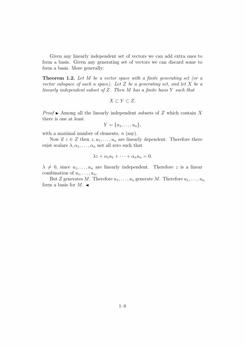
Given any linearly independent set of vectors we can add extra ones toform a basis. Given any generating set of vectors we can discard some toform a basis. More generally:
Theorem 1.2. Let M be a vector space with a finite generating set (or avector subspace of such a space). Let Z be a generating set, and let X be alinearly independent subset of Z. Then M has a finite basis Y such that
X ⊂ Y ⊂ Z.
Proof I Among all the linearly independent subsets of Z which contain Xthere is one at least
Y = u1, . . . , un,with a maximal number of elements, n (say).
Now if z ∈ Z then z, u1, . . . , un are linearly dependent. Therefore thereexist scalars λ, α1, . . . , αn not all zero such that
λz + α1u1 + · · ·+ αnun = 0.
λ 6= 0, since u1, . . . , un are linearly independent. Therefore z is a linearcombination of u1, . . . , un.
But Z generates M . Therefore u1, . . . , un generate M . Therefore u1, . . . , un
form a basis for M . J
1–8

Chapter 2
Linear Operators 1
2.1 The Definition
Definition. Let M, N be K-vector spaces. A map
MT→ N
is called a linear operator (or linear map or linear function or linear trans-formation or linear homomorphism) if
(i) T (x + y) = Tx + Ty (group homomorphism);
(ii) Tαx = αTx for all x, y ∈M, α ∈ K.
A linear operator is called a (linear) isomorphism if T is bijective. Wesay that M is isomorphic to N if there exists a linear isomorphism
M → N.
Note. Geometrically:
(i) means that T preserves parallelograms (see Figure 2.1);
(ii) means that T preserves collinearity (see Figure 2.2).
T(x+y) = Tx+Ty
y
x
x+y
Ty
Tx
2–1

Figure 2.1
Tx
x
0
Figure 2.2
Examples:
1. If
A = (αij) =
α11 . . . α1
n...
...αm
1 . . . αmn
∈ Km×n,
we denote by
Kn A→ Km
2–2

the linear operator given by matrix multiplication by A acting on ele-ments of Kn written as n× 1 columns. Since
A(x + y) = Ax + Ay,
Aαx = αAx
for matrix multiplication, it follows that A is a linear operator.E.g.
A =
(3 7 2−2 5 1
)
∈ R2×3
Now:
R3 → R2 :
αβγ
7→(
3α + 7β + 2γ−2α + 5β + γ
)
.
2. Taked
dt: C∞(R)→ C∞(R).
Now:
d
dt[x(t) + y(t)] =
d
dtx(t) +
d
dty(t),
d
dtcx(t) = c
d
dtx(t)
for all c ∈ R. Therefore ddt
is a linear operator.
3. The Laplacian
∆ =∂
∂x2+
∂
∂y2+
∂
∂z2: C∞(R3)→ C∞(R3)
is a linear operator.
2.2 Basic Properties of Linear Operators
1. If MT→ N is a linear operator and u1, . . . , ur ∈ M ; α1, . . . , αr ∈ K
thenT (α1u1 + · · ·+ αrur) = α1Tu1 + · · ·+ αrTur,
i.e.
T
r∑
i=1
αiui =
r∑
i=1
αiui,
i.e. T preserves linear combinations, i.e. T can be moved across sum-mations and scalars.
2–3

2. If MS,T→ N are linear operators, if u1, . . . , um generate M , and if Sui =
Tui (i = 1, . . . , m) then S = T .
Proof of This B Let x ∈M . Then x =∑m
i=1 αiui (say). Therefore
Sx = Sm∑
i=1
αiui =m∑
i=1
αiSui =m∑
i=1
αiTui = Tm∑
i=1
αiui = Tx.
C
Thus two linear operators which agree on a generating set must beequal.
3. Let u1, . . . , un be a basis for M , and w1, . . . , wn be arbitrary vectors inN . Then we can define a linear operator
MT→ N
byT (α1u1 + · · ·+ αnun) = α1w1 + · · ·+ αnun.
Thus T is the unique linear operator such that
Tui = wi (i = 1, . . . , m).
We say that T is defined by Tui = wi, and extended to M by linearity.
Definition. Let MT→ N be a linear operator. Then
ker T = x ∈ M : Tx = 0
is a vector subspace of M , called the kernel of M , and
im T = Tx : x ∈M
is a vector subspace of N , called the image of T . The dimension of im T iscalled the rank of T ,
rank T = dim im T.
2–4

2.3 Examples
1. Consider the matrix operator
Kn A→ Km,
where A ∈ Km×n,
A =
α11 α12 . . . α1n
......
αm1 αm2 . . . αmn
(say).ker T = x = (x1, . . . , xn) : Ax = 0
is the space of solutions of
α11 . . . α1n
......
αm1 . . . αmn
x1...
xn
=
0...0
,
i.e. The space of solutions of the m homogeneous linear equations in nunknowns, whose coefficients are the rows of A:
α11x1 + α12x2 + · · ·+ α1nxn = 0
...
αi1x1 + αi2x2 + · · ·+ αinxn = 0
...
αm1x1 + αm2x2 + · · ·+ αmnxn = 0
Number of equations = m = number of rows of A = dim Km.
Number of unknowns = n = number of columns of A = dim Kn.
We see that (x1, x2, . . . , xn) ∈ ker A iff the dot product:
(αi1, αi2, . . . , αin).(x1, . . . , xn) (i = 1, . . . , m)
with each row of A is zero. Therefore
ker A = (row A)⊥,
where row A is the vector subspace of Kn generated by the m rows ofA (see Figure 2.3).
Now row A is unchanged by the following elementary row operations:
2–5

(i) multiplying a row by a non-zero echelon;
(ii) interchanging rows;
(iii) adding to one row a scalar multiple of another row.
So ker A is also unchanged by these operations.
To obtain a basis for row A, and from this a basis for ker A, carry outelementary row operations in order to bring the matrix to row echelonform (i.e. so that each row begins with more zeros than the previousrow).
Example: Let
A =
2 1 −1 3−1 1 2 14 0 −1 2
: R4 → R3.
Now
A ∼
2 1 −1 30 3 3 50 −2 1 −4
2 row 2 + row 1row 3− 2 row 1
∼
2 1 −1 30 3 3 50 0 9 −2
3 row 3 + 2 row 2.
Since the new rows are in row echelon form they are linearly indepen-dent. Therefore row A is 3-dimensional, with basis (2, 1,−1, 3), (0, 3, 3, 5),(0, 0, 9,−2). Therefore
(α, β, γ, δ) ∈ ker A⇔ 2α + β − γ + 3δ = 0
3β + 3γ + 5δ = 0
9γ − 2δ = 0
⇔ γ = 29δ
3β = −3γ − 5δ = − 23δ − 5δ = −17
3δ
2α = −β + γ − 3δ = 179δ + 2
9δ − 3δ = −8
9δ
⇔ (α, β, γ, δ) = (− 49δ,−17
9δ, 2
9δ, δ) = δ
9(−4,−17, 2, 9)
Therefore ker A is 1-dimensional, with basis (−4,−17, 2, 9).
2–6
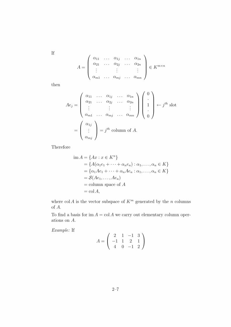
If
A =
α11 . . . α1j . . . α1n
α21 . . . α2j . . . α2n
......
...αm1 . . . αmj . . . αmn
∈ Km×n
then
Aej =
α11 . . . α1j . . . α1n
α21 . . . α2j . . . α2n
......
...αm1 . . . αmj . . . αmn
0·1·0
← jth slot
=
α1j
...αmj
= jth column of A.
Therefore
im A = Ax : x ∈ Kn= A(α1e1 + · · ·+ αnen) : α1, . . . , αn ∈ K= α1Ae1 + · · ·+ αnAen : α1, . . . , αn ∈ K= S(Ae1, . . . , Aen)
= column space of A
= col A,
where colA is the vector subspace of Km generated by the n columnsof A.
To find a basis for im A = col A we carry out elementary column oper-ations on A.
Example: If
A =
2 1 −1 3−1 1 2 14 0 −1 2
2–7

then
A ∼
2 0 0 0−1 3 3 54 −4 2 −8
2 col 2− col 12 col 3 + col 12 col 4− 3 col 1
∼
2 0 0 0−1 3 0 04 −4 6 −4
col 3− 2 col 23 col 4− 5 col 2
∼
2 0 0 0−1 3 0 04 −4 6 0
.
Therefore im A = col A has basis (2,−1, 4), (0, 3,−4), (0, 0, 6). There-fore rank A = dim im A = 3.
2. Let
D =d
dt: C∞(R)→ C∞(R) (Dx(t) =
d
dtx(t)).
(i) Let λ ∈ R and D − λ be the operator
(D − λ) =d
dtx(t)− λx(t).
Then
x ∈ ker(D − λ)⇔ (D − λ)x = 0⇔ dx
dt= λx⇔ x(t) = ceλt.
Therefore ker(D − λ) is 1-dimensional, with basis eλt.
(ii) To determine ker(D − λ)k we must solve:
(D − λ)kx = 0.
Put x(t) = eλty(t). Then
(D − λ)x = Dx(t)− λx(t)
= λeλty(t) + eλtDy(t)− λeλty(t)
= eλtDy(t).
Therefore
(D − λ)2x = eλtD2y(t)
...
(D − λ)kx = eλtDky(t).
2–8

Therefore
(D − λ)kx = 0⇔ eλtDky(t) = 0
⇔ Dky(t) = 0
⇔ y(t) = c0 + c1t + c2t2 + · · ·+ ck−1t
k−1
⇔ x(t) = (c0 + c1t + · · ·+ ck−1tk−1)eλt.
Therefore ker(D−λ)k is k-dimensional, with basis eλt, teλt, t2eλt, . . . , tk−1eλt.
2.4 Properties Continued
Theorem 2.1. Let MT→ N be a linear operator, where M is finite dimen-
sional. Let u1, . . . , uk be a basis for ker T , and let Tw1, . . . , Twr be a basisfor im T . Then
u1, . . . , uk, w1, . . . , wr
is a basis for M .
Proof I We have two things to show:
(i) Linear independence: Let
∑
αiui +∑
βjwj = 0
Apply T :
0 +∑
βjTwj = 0.
Therefore βj = 0 for all j. Therefore αi = 0 for all i.
Therefore u1, . . . , uk, w1, . . . , wr are linearly independent.
(ii) Generate: Let x ∈ M . Then
Tx =∑
βjTwj (say).
ThereforeTx = T
∑
βjwj.
ThereforeT [x−
∑
βjwj] = 0.
Thereforex−
∑
βjwj ∈ ker T.
2–9

Thereforex−
∑
βjwj =∑
αiui (say).
Thereforex =
∑
αiui +∑
βjwj.
Therefore u1, . . . , uk, w1, . . . , wr generate M . J
Corollary 2.1. dim ker T + dim im T = dim M .
Corollary 2.2. If dim M = dim N then
T is injective⇔ ker T = 0 ⇔ dim im T = dim N ⇔ T is surjective.
2.5 Operator Algebra
If M, N are K-vector spaces, we denote by
L(M, N)
the set of all linear operators M → N , and we denote by
L(M)
the set of all linear operators M →M .
Theorem 2.2. We have:
(i) L(M, N) is a K-vector space, with
(S + T )x = Sx + Tx,
(αT )x = α(Tx)
for all S, T ∈ L(M, N), x ∈M, α ∈ K.
(ii) Composition of operators gives a multiplication
L(L, M)× L(M, N) → L(L, N)(T, S) 7→ ST
LT→M
S→ N,
with(ST )x = S(Tx) for all x ∈ L,
which satisfies
(a) (RS)T = R(ST ),
2–10
(b) R(S + T ) = RS + RT ,
(c) (R + S)T = RT + ST ,
(d) (αS)T = α(ST ) = S(αT ),
provided each is well-defined.
Proof I Straight forward verification. J
Corollary 2.3. L(M) is
(i) a K-vector space: S + T, αS;
(ii) a ring: S + T, ST ;
(iii) (αS)T = α(ST ) = S(αT ) : αS, ST ,
i.e. L(M) is a K-algebra.
2.6 Isomorphisms of L(M, N) with Km×n
Definition. Let u1, . . . , un be a basis for M , and let w1, . . . , wm be a basis
for N . Let MT→ N . Put Then we have:
Tu1 = α11w1 + α2
1w2 + · · ·+ αi1wi + · · ·+ αm
1 wm,
...
Tuj = α1jw1 + α2
jw2 + · · ·+ αijwi + · · ·+ αm
j wm,
...
Tun = α1nw1 + α2
nw2 + · · ·+ αinwi + · · ·+ αm
n wm,
(say) where:
A = (αij) =
α11 α1
2 . . . α1j . . . α1
n...
......
αi1 . . . . . . αi
j . . . αin
......
...αm
1 . . . . . . αmj . . . αm
n
∈ Km×n.
Note. The coordinates of Tuj form the jth column of A - NOTE THETRANSPOSE! We call A the matrix of T wrt the bases u1, . . . , un for Mand w1, . . . , wm for N ,
Tuj =
m∑
i=1
αijωi.
2–11

Theorem 2.3. L(M, N)→ Km×n is a linear isomorphism where T → ma-trix of T w.r.t. basis u1, · · · , un; ω1, cdots, ωm.
Proof I Let T have matrix A = (αij), and let S have matrix B = (βi
j). Then
(T + S)uj = Tuj + Suj =
m∑
i=1
αijwi +
m∑
i=1
βijwi =
m∑
i=1
(αij + βi
j)wi.
Therefore T + S has matrix (αij + βi
j) = A + B. Also
(λT )uj = λ(Tuj) = λm∑
i=1
αijwi =
m∑
i=1
λαijwi.
Therefore λT has matrix (λαij) = λA. J
Corollary 2.4. dimL(M, N) = dim M. dim N .
Theorem 2.4. If LT→M has matrix A = (αi
j) wrt basis v1, . . . , vp, u1, . . . , un,
and MS→ N has matrix B = (βi
j) wrt basis u1, . . . , un, w1, . . . , wm then
LST→ N has basis
BA =
(n∑
k=1
βikα
kj
)
= (γij)
(say), wrt basis v1, . . . , vp, w1, . . . , wm.
Proof I
(ST )vj = S(Tvj) = S
(n∑
k=1
αkj uk
)
=
n∑
k=1
αkj Suk
=
n∑
k=1
αkj
m∑
i=1
βikwi =
m∑
i=1
(n∑
k=1
βikα
kj
)
wi =
m∑
i=1
γijwi.
J
Corollary 2.5. If dim M = n then each choice of basis u1, . . . , un of Mdefines an isomorphism of K-algebras:
L(M)→ Km : T 7→ matrix of T wrt u1, . . . , un.
Note. If MT→M has matrix A = (αi
j) wrt basis u1, . . . , un then
(i) Tuj =∑n
i=1 αijui, by definition;
2–12

(ii) the elements of the jth column of A are the coordinates of Tuj;
(iii) λ01 + λ1T + λ2T2 + · · ·+ λrT
r has matrix α0I + α1A + · · ·+ αrAr;
(iv) T−1 has matrix A−1,
since we have an algebra isomorphism.
Theorem 2.5. Let MT→ N have matrix A = (αi
j) wrt bases u1, . . . , un forM and w1, . . . , wm for N . Let x have coordinates
X = (ξi) =
ξ1
...ξn
wrt u1, . . . , un. Then Tx has coordinates
AX =
(m∑
i=1
αijξ
j
)
wrt w1, . . . , wm.
Proof I
Tx = T
(n∑
j=1
ξjuj
)
=
n∑
j=1
ξiTuj =
n∑
j=1
ξj
m∑
i=1
αijwi =
m∑
i=1
(n∑
j=1
αijξ
j
)
wi,
as required. J
Note. We have thus a commutative diagram:
MT−−−→ N
y
y
Kn A−−−→ Km
:x
T7→ Tx↓ ↓
x coord.A7→ Tx coord
2–13
Chapter 3
Changing Basis and EinsteinConvention
Definition. Ifold
u1, . . . , un andnew
w1, . . . , wn are two bases for M then we have:
u1 = p11w1 + p2
1w2 + · · ·+ pn1wn
...
uj = p1jw1 + p2
jw2 + · · ·+ pnj wn
...
un = p1nw1 + p2
nw2 + · · ·+ pnnwn
(say). Put
P = (pij) =
p11 . . . p1
j . . . p1n
p21 . . . p2
j . . . p2n
......
...pn
1 . . . p2j . . . pn
n
Note. The new coordinates of the old basis vector uj form the jth columnof P - NOTE THE TRANSPOSE! We call P the transition matrix from the(old) basis u1, . . . , un to the (new) basis w1, . . . , wn:
uj =n∑
i=1
pijwi.
Theorem 3.1. If x has old coordinates
X = (ξi) =
ξ1
...ξn
3–1

then x has new coordinates
PX =
n∑
j=1
(pijξ
j) = (ηi)
(say).
Proof I
x =
n∑
j=1
ξjuj =
n∑
j=1
ξj
n∑
i=1
pijwi =
n∑
i=1
(n∑
j=1
pijξ
j
)
wi =
n∑
i=1
ηiwi.
J
We shall often use the Einstein summation convention (s.c.) when deal-ing with basis and coordinates in a fixed n-dimensional vector space M .Repeated indices (one up, one down) are summed from 1 to n (contractionof repeated indices). Non-repeated indices may take each value 1 to n.
Example:
• αi denotes
α1
...αn
(column matrix; upper index labels the row).
• αi denotes
(α1, . . . , αn) (row matrix; lower index labels the column).
• αij denotes
α11 . . . α1
n...
...αn
1 . . . αnn
(square matrix).
• ui denotes u1, . . . , un (basis).
• αiui denotes α1u1 + · · ·+ αnun.
• αiβi denotes α1β1 + · · ·+ αnβn (dot product).
3–2

• αikβ
kj denotes AB (matrix product).
AlsoTuj = αi
jui (αij matrix of operator T )
anduj = pi
jwi (pij transition matrix from ui to wi).
If x has components ξi wrt ui then Tx has components αijξ
i wrt ui. If x hascomponents ξj wrt ui then x has components pi
jξj wrt wi.
• δij denotes the unit matrix
I =
1 0 . . . 00 1 . . . 0...
. . ....
0 . . . 0 1
.
• If Q = P−1 then (qij) denotes Q (inverse matrix) and
qikp
kj = δi
j = pikq
kj .
Theorem 3.2. Let MT→ N have matrix A wrt basis u1, . . . , un. Let P be
the transition matrix to (new) basis w1, . . . , wn. Then T has (new) matrix
PAP−1
wrt w1, . . . , wn.
Proof I Let P = (pij), A = (αi
j), P−1 = Q = (qij). Then
Tuj = αijui; uj = pi
jwi; wj = qijui.
Therefore
Twj = Tqljul = ql
jTul = qljα
kl uk = ql
jαkl p
ikwi = pi
kαkl q
lj
︸ ︷︷ ︸
PAP−1
wi,
as required. J
3–3

Chapter 4
Linear Forms and Duality
4.1 Linear Forms
Definition. Fix M a K-vector space. A scalar valued linear function
f : M → K
is called a linear form on M .
If f is a linear form on M , and x is a vector in M , we write
〈f, x〉
to denote the value of f on x. This notation has the advantage of treating fand x in a symmetrised way:
(i) 〈f, x + y〉 = 〈f, x〉+ 〈f, y〉,
(ii) 〈f + g, x〉 = 〈f, x〉+ 〈g, x〉,
(iii) 〈αf, x〉 = α〈f, x〉 = 〈f, αx〉,
(iv)⟨∑r
i=1 αifi,∑s
j=1 βjxj
⟩
=∑r
i=1
∑s
j=1 αiβj〈f i, xj〉.
If M is finite dimensional, with basis u1, . . . , un, then each x ∈ M can bewritten uniquely as
x = α1u1 + · · ·+ αnun =n∑
i=1
αiui = αiui.
We write〈ui, x〉 = αi
4–1

to denote the ith coordinate of x wrt basis u1, . . . , un. We have:
〈ui, x + y〉 = 〈ui, x〉+ 〈ui, y〉,〈ui, αx〉 = α〈ui, x〉.
Thus ui is a linear form on M , called the ith coordinate function wrt basisu1, . . . , un. We have:
1. 〈ui, uj〉 =
1 if i = j0 if i 6= j
= δij (Kronecker delta);
2. x =∑n
i=1〈ui, x〉ui for all x ∈M ;
3. 〈α1u1 + · · · + αnun, β1u1 + · · · + βnun〉 = α1β
1 + · · · + αnβn = αiβi
(dot product).
Theorem 4.1. If u1, . . . , un is a basis for M then the coordinate functionsu1, . . . , un form a basis for the space M ∗ of linear forms on M (called thedual space of M), called the dual basis, and
f =n∑
i=1
〈f, ui〉ui for each f ∈M ∗.
Proof I We have to show that u1, . . . , un generate M , and are linearly inde-pendent.
(i) Generate: Let f ∈M ∗; 〈f, uj〉 = βj (say). Then
⟨n∑
i=1
βiui, uj
⟩
=n∑
i=1
βi〈ui, uj〉 =n∑
i=1
βiδij = βj = 〈f, uj〉.
Therefore∑n
i=1 βiui and f are linear forms on M which agree on the
basis vectors u1, . . . , un. Therefore
f =n∑
i=1
βiui =
n∑
i=1
〈f, ui〉ui.
(ii) Linear independence: Let∑n
i=1 βiui = 0. Then
⟨n∑
i=1
βiui, uj
⟩
= 0
4–2

for all j = 1, . . . , n. Therefore
n∑
i=1
βiδij = 0
for all j = 1, . . . , n. Therefore βj = 0 for all j = 1, . . . , n. Thereforeu1, . . . , un are linearly independent. J
Corollary 4.1. dim M∗ = dim M .
Note. We denote by x, y, z the coordinate function on K3 wrt basis e1, e2, e3,and we denote by x1, . . . , xn the coordinate function on Kn wrt basis e1, . . . , en.These coordinates are called the usual coordinates.
4.2 Duality
Let M be finite dimensional, with dual space M ∗. If x ∈ M and f ∈ M∗
then
(i) f is a linear form on M whose value on x is 〈f, x〉;
(ii) we identify x with the linear form on M ∗ whose value on f is 〈f, x〉:f = 〈f, ·〉,x = 〈·, x〉.
What we are doing is identifying M with the dual of M ∗, by means ofthe linear isomorphism:
M →M∗∗
x 7→ 〈·, x〉.This is a linear map, and is bijective because:
(i) dim M∗∗ = dim M∗ = dim M ,
(ii) 〈·, x〉 = 0 ⇒ 〈ui, x〉 = 0 for all x ⇒ x = 0. So the map is injective(kernel = 0), and hence by (i) surjective.
If u1, . . . , un is a basis for M , and u1, . . . , un the dual basis for M ∗ then
〈ui, uj〉 = δij
shows that u1, . . . , un is the basis dual to u1, . . . , un.The identification of vectors x ∈ M as linear forms on M ∗ is called
duality. A basis u1, . . . , un for M∗ is called a linear coordinate system on M ,and consists of coordinate functions wrt its dual basis u1, . . . , un.
4–3

4.3 Systems of Linear Equations
Definition. If f 1, . . . , fk are linear forms on M then we consider the vectorsubspace of M on which
f 1 = 0, . . . , f k = 0 (∗).
Any vector in this subspace is called a solution of the equations (∗). Thusx ∈ M is a solution iff
〈f 1, x〉 = 0, . . . , 〈f k, x〉 = 0.
The set of solutions is called the solution space of the system of k homoge-neous equations (∗). The dimension of the space S(f 1, . . . , fk) generated byf 1, . . . , fk is called the rank (number of linearly independent equations) ofthe system of equations.
In particular, if u1, . . . , un is a linear coordinate system on M then wecan write the equations as:
f 1 ≡ β11u
1 + · · ·+ β1nun = 0
...
fk ≡ βk1u1 + · · ·+ βk
nun = 0
The coordinate map M ∗ → Kn maps
f 1 7→ (β11 , . . . , β
1n)
...
fk 7→ (βk1 , . . . , βk
n).
Thus it maps S(f 1, . . . , fk) isomorphically onto the row space of B = (β ij).
Therefore
rank of system = dimension of row space of B = dim row B.
Example: The equations
3x− 4y + 2z = 0,
2x + 7y + 3z = 0,
where x, y, z are the usual coordinates on R3, have
rank = dim row
(3 −4 22 7 3
)
= 2.
4–4

Theorem 4.2. A system of k homogeneous linear equations of rank r on ann-dimensional vector space M has a solution space of dimension n− r.
Proof I Letf 1 = 0, . . . , f k = 0
be the system of equations. Let u1, . . . , ur be a basis for S(f 1, . . . , fk). Ex-tend to a basis u1, . . . , ur
equations, ur+1, . . . , un for M∗. Let u1, . . . , ur, ur+1, . . . , un
solutions
be
the dual basis of M . Then
x = α1u1 + · · ·+ αrur + αr+1ur+1 + · · ·+ αnun ∈ solution space
⇔ α1 = 〈u1, x〉 = 0, . . . , αr = 〈ur, x〉 = 0
⇔ x = αr+1ur+1 + · · ·+ αnun.
Therefore ur+1, . . . , un is a basis for the solution space. Therefore solutionspace has dimension n− r. J
Theorem 4.3. Let B ∈ Kk×n, where K is a field. Then
dim row B = dim colB (= rank B).
Proof I Consider the k homogeneous linear equations on Kn with coefficientsB = (βi
j):
β11x
1 + · · ·+ β1nxn = 0
...
βk1x1 + · · ·+ βk
nxn = 0.
Now
n− dim row B = n− rank of equations
= dimension of solution space
= dim ker B
= n− dim im B
= n− dim col B.
Therefore dim col B = dim row B. J
4–5

Chapter 5
Tensors
5.1 The Definition
Definition. Let M be a finite dimensional vector space over a field K, letM∗ be the dual space, and let dim M = n. A tensor over M is a function ofthe form
T : M1 ×M2 × · · · ×Mk → K,
where each Mi = M or M∗ (i = 1, . . . , k), and which is linear in each variable(multilinear).
Two tensors S, T are said to be of the same type if they are defined onthe same set M1 × · · · ×Mk.
Example: A tensor of type
T : M ×M∗ ×M → K
is a scalar valued function T (x, f, y) of three variables (x a vector, f a linearform, y a vector) such that
T (αx + βy, f, z) = αT (x, f, z) + βT (y, f, z) linear in 1st variable,
T (x, αf + βg, z) = αT (x, f, z) + βT (x, g, z) linear in 2nd variable,
T (x, f, αy + βz) = αT (x, f, z) + βT (x, f, z) linear in 3rd variable.
If ui is a basis for M , and ui is the dual basis for M ∗ then the array ofn3 scalars
αijk = T (ui, u
j, uk)
are called the components of T .
5–1

If x, f, y have components ξi, ηj, ρk respectively then
T (x, f, y) = T (ξiui, ηjuj, ρkuk) = ξiηjρ
kT (ui, uj, uk) = ξiηjρ
kαijk
(using summation notation), i.e. the components of T contracted by thecomponents of x, f, y.
The set of all tensors over M of a given type form a K-vector space if wedefine
(S + T )(x1, . . . , xk) = S(x1, . . . , xk) + T (x1, . . . , xk),
(λT )(x1, . . . , xk) = λ(T (x1, . . . , xk)).
The vector space of all tensors of type
M ×M∗ ×M → K
(say) has dimension n3, since T 7→ T (ui, uj, uk) (components of T ) maps it
isomorphically onto Kn3.
Definition. If S : M1 × · · · ×Mk → K and T : Mk+1 × · · · ×Ml → K aretensors over M then we define their tensor product S ⊗ T to be the tensor:
S ⊗ T : M1 × · · · ×Mk ×Mk+1 × · · · ×Ml → K,
whereS ⊗ T (x1, . . . , xl) = S(x1, . . . , xk)T (xk+1, . . . , xl).
Example: If S has components αijk, and T has components βrs then S ⊗ T
has components αijkβ
rs, because
S ⊗ T (ui, uj, uk, u
r, us) = S(ui, uj, uk)T (ur, us).
Tensors satisfy algebraic laws such as:
(i) R⊗ (S + T ) = R⊗ S + R⊗ T ,
(ii) (λR)⊗ S = λ(R⊗ S) = R⊗ (λS),
(iii) (R⊗ S)⊗ T = R⊗ (S ⊗ T ).
ButS ⊗ T 6= T ⊗ S
in general. To prove those we look at components wrt a basis, and note that
αijk(β
rs + γr
s) = αijkβ
rs + αi
jkγrs,
for example, butαiβj 6= βjαi
in general.
5–2

5.2 Contraction
Definition. Let T : M1 × · · · ×Mr × · · · ×Ms× · · · ×Mk → K be a tensor,with
Mr = M∗, Ms = M
(say). Then we can contract the rth index of T with the sth index to get anew tensor
S : M1 × · · · ×omit
Mr × · · · ×omit
Ms × · · · ×Mk → K
defined by
S(x1, x2, . . . , xk−2) = T (x1, . . . , ui
rth slot, . . . , ui
sth slot
, . . . , xk−2),
where ui is a basis for M .
To show that S is well-defined we need:
Theorem 5.1. The definition of contraction is independent of the choice ofbasis.
Proof I PutR(f, x) = T (x1, x2, . . . , f, . . . , x, . . . , xk−2).
Then if ui, wi are bases:
R(wi, wi) = R(piku
k, qliul) = pi
kqliR(uk, ul) = δl
kR(uk, ul) = R(uk, uk),
as required. J
Example: If T has components αijk
lm wrt basis ui then contraction of the2nd and 4th indices gives a tensor with components
βikm = T (ui, uj, uk, u
j, um) = αijk
jm.
Thus when we contract we eliminate one upper (contravariant) index andone lower (covariant) index.
5.3 Examples
A vector x ∈M is a tensor:
x : M∗ → K
5–3

with components αi = 〈ui, x〉 (one contravariant index).A linear form f ∈M ∗ is a tensor:
f : M → K
with components αi = 〈f, ui〉 (one covariant index).A tensor with two covariant indices:
T : M ×M → K,
with T (ui, uj) = αij, is called a bilinear form or scalar product.
Example: The dot product
Kn ×Kn → K
((α1, . . . , αn), (β1, . . . , βn)) 7→ α1β1 + · · ·+ αnβn
is a bilinear form on Kn.If M
T→M is a linear operator, we shall identify it with the tensor:
T : M∗ ×M → K
byT (f, x) = 〈f, Tx〉.
This tensor has components
αij = T (ui, uj) = 〈ui, Tuj〉 = matrix of linear operator T
(one contravariant index, one covariant index).
Note (The Transformation Law). Let pij be the transition matrix from
basis ui to basis wi, with inverse matrix qji . Let T be a tensor M×M ∗×M →
K (say). Then
new comps.︷ ︸︸ ︷
T (wi, wj, wk) = T (qr
i ur, pjsu
s, qtkut) = qr
i pjsq
tk
old comps.︷ ︸︸ ︷
T (ur, us, ut),
i.e. Upper indices contract with p, lower indices contract with q.
5–4

5.4 Bases of Tensor Spaces
Let M ×M∗×M → K (∗) (say) be a tensor with components αijk wrt basis
ui. Then the tensor:αi
jk ui ⊗ uj ⊗ uk (∗∗)
is of the same type as T , and has components
αijku
i ⊗ uj ⊗ uk[ur, us, ut] = αi
jk〈ui, ur〉〈us, uj〉〈uk, ut〉
= αijkδ
irδ
sjδ
kt
= αrst.
Therefore (∗∗) has the same components as T . Therefore
T = αijk ui ⊗ uj ⊗ uk.
Therefore ui ⊗ uj ⊗ uk is a basis for the n3-dimensional space of all tensorsof type (∗).
5–5

Chapter 6
Vector Fields
6.1 The Definition
Let V be an open subset of Rn. Let x1, . . . , xn be the usual coordinate
functions on Rn. Let Vf→ R. If a = (a1, . . . , an) ∈ V then we define the
partial derivative of f wrt ith variable at a:
∂f
∂xi(a) = lim
t→0
f(a1, . . . , ai + t, . . . , an)− f(a1, . . . , ai, . . . , an)
t
= limt→0
f(a + tei)− f(a)
t
=d
dtf(a + tei)|t=0
(see Figure 6.1). If it exists for each a ∈ V then we have:
∂f
∂xi: V → R.
6–1

a+te
a V
Figure : 6.1
Note that∂xi
∂xj= δi
j.
If all repeated partial derivatives of all orders:
∂rf
∂xi1 · · ·∂xir=
∂
∂xi1. . .
∂
∂xirf : V → R
exist we call f C∞. We denote by C∞(V ) the space of all C∞ functionsV → R. C∞(V ) is an R-algebra:
(i) (f + g)(x) = f(x) + g(x),
(ii) (fg)(x) = f(x)g(x),
(iii) (αf)(x) = α(f(x)).
Each sequence α1, . . . , αn of elements of C∞(V ) defines a linear operator
v = α1 ∂
∂x1+ · · ·+ αn ∂
∂xn
6–2

on C∞(V ), where
(vf)(x) = α1(x)∂f
∂x1(x) + · · ·+ αn(x)
∂f
∂xn(x).
Such an operatorv : C∞(V )→ C∞(V )
is called a (contravariant) vector field on V .Now for each fixed a we denote by
∂
∂xia
the operator given by:∂
∂xia
f =∂f
∂xi(a).
Thus ∂∂xi
aacts on any function f which is defined and C1 on an open set
containing a. We define the linear combination∑n
i=1 αi ∂∂xi
aby
(
α1 ∂
∂xia
+ · · ·+ αn ∂
∂xna
)
f = α1 ∂f
∂x1(a) + · · ·+ αn ∂f
∂xn(a).
The set of linear combinations
α1 ∂
∂x1a
+ · · ·+ αn ∂
∂xna
: α1, . . . , αn ∈ R
is called the tangent space to Rn at a, denoted TaRn. Thus TaR
n is a realn-dimensional vector space, with basis
∂
∂x1a
, . . . ,∂
∂xna
.
The operators ∂∂xi
aare linearly independent, since
α1 ∂
∂x1a
+ · · ·+ αn ∂
∂xna
= 0⇒(
α1 ∂
∂x1a
+ · · ·+ αn ∂
∂xna
)
xi = 0⇒ αi = 0,
since ∂xi
∂xj (a) = δij.
If v = α1 ∂∂x1 + · · ·+ αn ∂
∂xn (αi ∈ C∞(V )) is a vector field on V then wehave (see Figure 6.2), for each x ∈ V a tangent vector
vx = α1(x)∂
∂x1x
+ · · ·+ αn(x)∂
∂xnx
∈ TxRn.
6–3

v
V
x
Figure 6.2
We call vx the value of v at x, and note that
vxf =
(
α1(x)∂
∂x1x
+ · · ·+ αn(x)∂
∂xnx
)
f
= α1(x)∂f
∂x1(x) + · · ·+ αn(x)
∂f
∂xn(x)
= (vf)(x)
for all x ∈ V . Thus v is determined by its values vx : x ∈ V , and viceversa. Thus a contravariant vector field is a function on V
x 7→ vx,
which maps to each point x ∈ V a tangent vector vx ∈ TxRn.
6.2 Velocity Vectors
β(t)
6–4

Figure 6.3
Let β(t) = (β1(t), . . . , βn(t)) be a sequence of real valued C∞ functionsdefined on an open subset of R. Thus β = (β1, . . . , βn) is a curve in Rn (seeFigure 6.3). If f is a C∞ real-valued function on an open set in Rn containingβ(t) then the rate of change of f along the curve β at parameter t is
d
dtf(β(t)) =
d
dtf(β1(t), . . . , βn(t))
=∂f
∂x1(β(t))
d
dtβ1(t) + · · ·+ ∂f
∂xn(β(t))
d
dtβn(t) (by the chain rule)
=
[
d
dtβ1(t)
∂
∂x1β(t)
+ · · ·+ d
dtβn(t)
∂
∂xnβ(t)
]
f
=.
β(t)f,
where.
β(t) =d
dtβ1(t)
∂
∂x1β(t)
+ · · ·+ d
dtβn(t)
∂
∂xnβ(t)
∈ Tβ(t)Rn
is called the velocity vector of β at t.We note that if β(t) has coordinates
βi(t) = xi(β(t))
then.
β(t) has components
d
dtβi(t) =
d
dtxi(β(t))
= rate of change of xi along β at t wrt basis ∂∂x1
β(t), . . . , ∂
∂xnβ(t)
.
In particular, if α = (α1, . . . , αn) ∈ Rn and a = (a1, . . . , an) ∈ Rn then thestraight line through a (see Figure 6.4) in the direction of α:
(a1 + tα1, . . . , an + tαn)
a
tα
Figure 6.4
6–5

has velocity vector at t = 0:
α1 ∂
∂x1a
+ · · ·+ αn ∂
∂xna
∈ TaRn.
Thus each tangent vector is a velocity vector.
6.3 Differentials
Definition. If a ∈ Rn, and f is a C∞ function on an open neighbourhoodof a then the differential of f at a, denoted
dfa,
is the linear form on TaRn defined by
〈dfa,.
β(t)〉 =d
dtf(β(t)) =
.
β(t)f
a
β(t)
= β(t)
Figure 6.5
for any velocity vector.
β(t), such that β(t) = a.
Thus
(i) 〈dfβ(t),.
β(t)〉 = rate of change of f along β at t (see Figure 6.5),
(ii) 〈dfa, v〉 = vf (for all v ∈ TaRn) = rate of change of f along v.
Theorem 6.1. dxia, . . . , dxn
a is the basis of TaRn∗ dual to the basis ∂
∂x1a, . . . , ∂
∂xna
for TaRn.
Proof I⟨
dxia,
∂
∂xja
⟩
=∂xi
∂xj(a) = δi
j,
as required. J
6–6
Definition. If V is open in Rn then a covariant vector field ω on V is afunction on V :
ω : x 7→ ωx ∈ TxRn∗.
The covariant vector fields on V can be added:
(ω + η)x = ωx + ηx,
and multiplied by elements of C∞(V ):
(fω)x = f(x)ωx.
Each covariant vector field ω on V can be written uniquely as
ωx = β1(x)dx1x + · · ·+ βn(x)dxn
x.
Thusω = β1dx1 + · · ·+ βndxn
(we confine ourselves to βi ∈ C∞(V )).If f ∈ C∞(V ) then the covariant vector field
df : x 7→ dfx
is called the differential of f . Thus we have:
• contravariant vector fields:
v = α1 ∂
∂x1+ · · ·+ αn ∂
∂xn, αi ∈ C∞(V );
• covariant vector fields:
ω = β1dx1 + · · ·+ βndxn, β ∈ C∞(V );
and more general tensor fields, e.g.
S = αijk dxi ⊗ ∂
∂xj⊗ dxk, αi
jk ∈ C∞(V ),
a function on V whose value at x is
Sx = αijk(x)dxi
x ⊗∂
∂xjx
⊗ dxkx,
a tensor over TxRn.We can add, multiply and contract tensor fields pointwise (carrying out
the operation at each point x ∈ V ). For example:
6–7

(i) (R + S)x = Rx + Sx,
(ii) (R⊗ S)x = Rx ⊗ Sx,
(iii) (contracted S)x = contracted (Sx),
(iv) (fS)x = f(x)Sx f ∈ C∞(V ).
Contracting the covariant vector field ω = β1dx1 + · · ·+ βndxn with thecontravariant vector field v = α1 ∂
∂x1 + · · ·+ αn ∂∂xn gives the scalar field
〈ω, v〉 = β1α1 + · · ·+ βnαn.
In particular, if f ∈ C∞(V ) has differential df then the scalar field
〈df, v〉 = vf
is the rate of change of f along v.If ω = β1dx1 + · · ·+ βndxn then
βi = ith component of ω =
⟨
ω,∂
∂xi
⟩
.
In particular:
ith compoment of df =
⟨
df,∂
∂xi
⟩
=∂f
∂xi.
Therefore
df =∂f
∂x1dx1 + · · ·+ ∂f
∂xndxn Chain Rule,
rate of change of f =∂f
∂x1.rate of change of x1 + · · ·+ ∂f
∂xn.rate of change of xn.
6.4 Transformation Law
A sequencey = (y1, . . . , yn) (yi ∈ C∞(V ))
is called a (C∞) coordinate system on V if
V →W
x 7→ y(x) = (y1(x), . . . , yn(x))
6–8

maps V homeomorphically onto an open set W in Rn, and if
xi = F i(y1, . . . , yn),
where F i ∈ C∞(W ).
(r,r
(x,y)
r
(r,π
θ)θ)
θθ
−π
Figure 6.6
Example: (r, θ) is a C∞ coordinate system on (x, y) : y or x > 0 (see Figure6.6), where r =
√
x2 + y2, θ unique solution of x = r cos θ, y = r sin θ (−π <θ < π).
If a ∈ V , and β is the parametrised curve – the curve along which allyj (j 6= i) are constant, and yi varies by t – such that
y(β(t)) = y(a) + tei
y(a)+te
W
V
a
y(a)y
6–9

i
Figure 6.7
(see Figure 6.7) then the velocity vector of β at t = 0 is denoted:
∂
∂yia
Thus if f is C∞ in a neighbourhood of a then
∂f
∂yi(a) =
∂
∂yia
f =d
dtf(β(t))|t=0 = rate of change of f along the curve β.
If we write f as a function of y1, . . . , yn:
f = F (y1, . . . , yn)
(say), then
∂f
∂yi(a) =
d
dtf(β(t))|t=0 =
d
dtF (y(β(t)))|t=0 =
d
dtF (y(a)+tei)|t=0 =
∂F
∂xi(y(a)),
i.e. to calculate ∂f
∂yi (a) write f as a function F of y1, . . . , yn, and calculate∂F∂xi (partial derivative of F wrt ith slot):
∂f
∂yi=
∂F
∂xi(y1, . . . , yn).
Now if β is any parametrised curve at a, with β(t) = a (see Figure 6.8),then
〈dfa,.
β(t)〉 =d
dtf(β(t))
=d
dtF (y1(β(t)), . . . , yn(β(t)))
=n∑
i=1
∂F
∂xi(y1(β(t)), . . . , yn(β(t)))
d
dtyi(β(t))
=
n∑
i=1
∂f
∂yi(β(t))〈dyi
a,.
β(t)〉
6–10
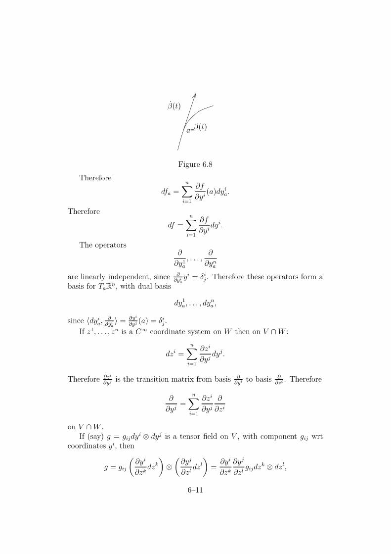
a=
β(t)
β(t)
Figure 6.8
Therefore
dfa =
n∑
i=1
∂f
∂yi(a)dyi
a.
Therefore
df =n∑
i=1
∂f
∂yidyi.
The operators∂
∂y1a
, . . . ,∂
∂yna
are linearly independent, since ∂∂yi
ayi = δi
j. Therefore these operators form abasis for TaR
n, with dual basis
dy1a, . . . , dyn
a ,
since 〈dyia,
∂∂yi
a〉 = ∂yi
∂yj (a) = δij.
If z1, . . . , zn is a C∞ coordinate system on W then on V ∩W :
dzi =n∑
i=1
∂zi
∂yjdyj.
Therefore ∂zi
∂yj is the transition matrix from basis ∂∂yi to basis ∂
∂zi . Therefore
∂
∂yj=
n∑
i=1
∂zi
∂yj
∂
∂zi
on V ∩W .If (say) g = gijdyi ⊗ dyj is a tensor field on V , with component gij wrt
coordinates yi, then
g = gij
(∂yi
∂zkdzk
)
⊗(
∂yj
∂zldzl
)
=∂yi
∂zk
∂yj
∂zlgijdzk ⊗ dzl,
6–11

using s.c., and therefore g has component
∂yi
∂zk
∂yj
∂zlgij
wrt coordinates zi.
Example: On Rn:
(i) usual coordinates x, y;
(ii) polar coordinates r, θ.
x = r cos θ, y = r sin θ.
So
dx =∂x
∂rdr +
∂x
∂θdθ = cos θ dr − r sin θ dθ,
dy =∂y
∂rdr +
∂y
∂θdθ = sin θ dr + r cos θ dθ.
The matrix (cos θ −r sin θsin θ r cos θ
)
is the transition matrix from r, θ to x, y:
∂
∂r=
∂x
∂r
∂
∂x+
∂y
∂r
∂
∂y= cos θ
∂
∂x+ sin θ
∂
∂y,
∂
∂θ=
∂x
∂θ
∂
∂x+
∂y
∂θ
∂
∂y= −r sin θ
∂
∂x+ r cos θ
∂
∂y.
6–12

Chapter 7
Scalar Products
7.1 The Definition
Definition. A tensor of type M × M → K is called a scalar product or(bilinear form) (i.e. two lower indices).
Example: The dot product Kn ×Kn → K. Writing X, Y as n× 1 columns:
((α1, . . . , αn), (β1, . . . , βn)) 7→ α1β1 + · · ·+ αnβn
(X, Y ) 7→ X tY.
7.2 Properties of Scalar Products
1. If (·|·) is a scalar product on M with components G = (gij) wrt basisui, if x has components X = (φi) and y has components Y = (νi)(gij = (ui|uj) and (·|·) = giju
i ⊗ uj) then
(x|y) = (φiui|νjuj)
= φiνj(ui|uj)
= gijφiνj
=(
φ1 . . . φn)
g11 . . . g1n
......
gn1 . . . gnn
ν1
...νn
= X tGY.
Note. The dot product has matrix I wrt ei, since ei.ej = δij.
7–1

2. If P = (pij) is the transition matrix to new basis wi then new matrix of
(·|·) is QtGQ, where Q = P−1.
Proof of This B As a tensor with two lower indices, new components
of (·|·) are:qki ql
jgkl = qki gklq
lj = QtGQ.
Check:(PX)tQtGQ(Y ) = X tP tQtGQY = X tGY.
C
3. (·|·) is called symmetric if
(x|y) = (y|x)
for all x, y. This is equivalent to G being a symmetric matrix Gt = G:
gij = (ui|uj) = (uj|ui) = gji.
A symmetric scalar product defines an associated quadratic form
F : M → K
by
F (x) = (x|x)
= X tGX
=(
ξ1 . . . ξn)
g11 . . . g1n
......
gn1 . . . gnn
ξ1
...ξn
= gijξiξj,
i.e.
F =(
u1 . . . un)
g11 . . . g1n
......
gn1 . . . gnn
u1
...un
= gijuiuj.
uiuj is a product of linear forms, and is a function:
(uiuj)(x) = ui(x)uj(x).
7–2

Example: If x, y, z are coordinate functions on M then
F =(
x y z)
3 2 32 −7 −13 −1 2
xyz
= 3x2 − 7y2 + 2z2 + 4xy + 6xz − 2yz.
(Thus quadratic form ≡ homogeneous 2nd degree polynomial).
The quadratic form F determines the symmetric scalar product (·|·)uniquely because:
(x + y|x + y) = (x|x) + (x|y) + (y|x) + (y|y),
2(x|y) = F (x + y)− F (x)− F (y) ( if 1 + 1 6= 0),
and gij = (ui|uj) are called the components of F wrt ui.
Definition. (·|·) is called non-singular if
(x|y) = 0 for all y ∈M ⇒ x = 0,
i.e.X tGY = 0 for all Y ∈ Kn ⇒ X = 0,
i.e.X tG = 0⇒ X = 0,
i.e.det G 6= 0.
Definition. A tensor field (·|·) with two lower indices on an open set V ⊂ Rn:
(·|·) = gijdyi ⊗ dyj
(say), yi coordinates on V , is called a metric tensor if
(·|·)x
is a symmetric non-singular scalar product on TxRn for each x ∈ V , i.e.
gij = gji and det gij nowhere zero.
The associated field ds2 of quadratic forms:
ds2 = gijdyidyj
is called the line-element associated with the metric tensor.
7–3
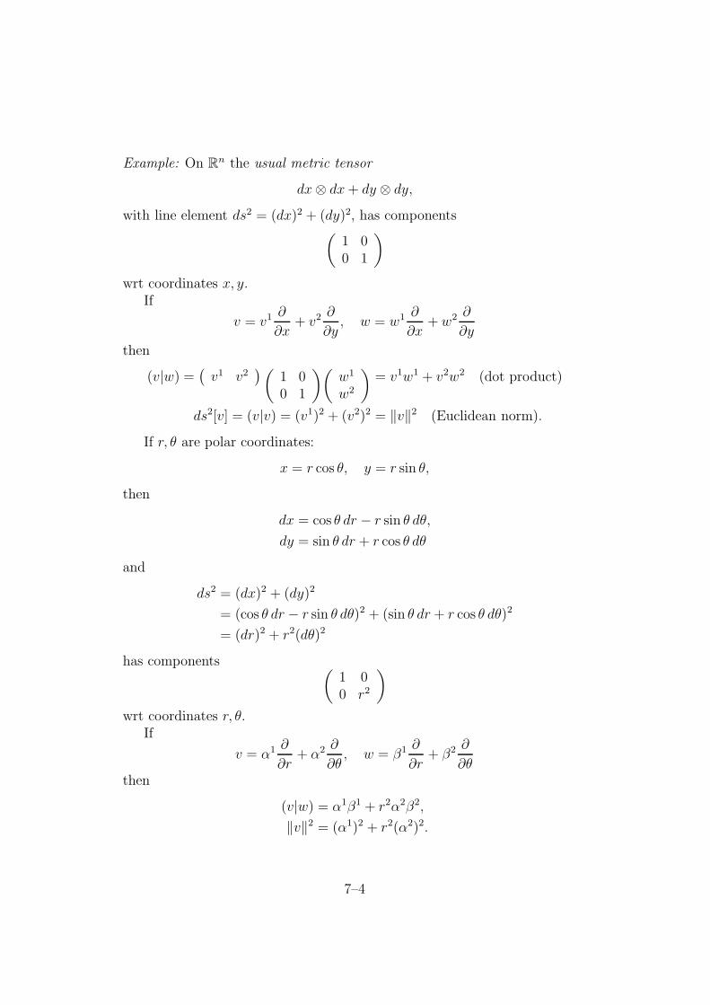
Example: On Rn the usual metric tensor
dx⊗ dx + dy ⊗ dy,
with line element ds2 = (dx)2 + (dy)2, has components(
1 00 1
)
wrt coordinates x, y.If
v = v1 ∂
∂x+ v2 ∂
∂y, w = w1 ∂
∂x+ w2 ∂
∂y
then
(v|w) =(
v1 v2)(
1 00 1
)(w1
w2
)= v1w1 + v2w2 (dot product)
ds2[v] = (v|v) = (v1)2 + (v2)2 = ‖v‖2 (Euclidean norm).
If r, θ are polar coordinates:
x = r cos θ, y = r sin θ,
then
dx = cos θ dr − r sin θ dθ,
dy = sin θ dr + r cos θ dθ
and
ds2 = (dx)2 + (dy)2
= (cos θ dr − r sin θ dθ)2 + (sin θ dr + r cos θ dθ)2
= (dr)2 + r2(dθ)2
has components (1 00 r2
)
wrt coordinates r, θ.If
v = α1 ∂
∂r+ α2 ∂
∂θ, w = β1 ∂
∂r+ β2 ∂
∂θthen
(v|w) = α1β1 + r2α2β2,
‖v‖2 = (α1)2 + r2(α2)2.
7–4
7.3 Raising and Lowering Indices
Definition. Let M be a finite dimensional vector space with a fixed non-singular symmetric scalar product (·|·). If x ∈ M is a vector (one upperindex), we associate with it
x ∈M∗,
a linear form (one lower index) defined by:
〈x, y〉 = (x|y) for all y ∈M.
We call the operation
M →M∗
x 7→ x
lowering the index. Thus
x ≡ (x|·) ≡ ‘take scalar product with x,.
If x = αiui has components αi then x has components
αj = 〈x, uj〉 = (x|uj) = (αiui|uj) = αi(ui|uj) = αigij.
Since (·|·) is non-singular, gij is invertible, with inverse gij (say), and we have
αj = αigij.
Thus
M →M∗
x 7→ x
is a linear isomorphism, with inverse
f∼
← f
(say), called raising the index. So
x = αiui = f∼
,
x = αiui = f
and(x|y) = (f
∼
|y) = 〈f, y〉 = 〈x, y〉.
7–5
To lower: contract with gij (αj = αigij).
To raise: contract with gij (αj = αigij).
Let MT→ M be a linear operator and (·|·) be symmetric. The matrix of
T is:αi
j = 〈ui, Tuj〉,one up, one down mixed components of T.
αij = (ui|Tuj),
two down covariant components of T.
αij = (ui|αkjuk) = (ui|uk)α
kj = gikα
kj
(lower by contraction with gij). Therefore
αij = gikαkj
(raise by contraction with gij).If we take the covariant components αij, and raise the second index we
getαi
j = αikgkj.
αij are the components of the tensor B (two lower indices) defined by:
B(x, y) = (x|Ty),
sinceB(ui, uj) = (ui|Tuj) = αij.
αji are the components of an operator T ∗ (one upper index, one lower
index) defined by:(T ∗x|y) = (x|Ty),
since T ∗ has components
γij = (ui|T ∗uj) = (T ∗uj|ui) = (uj|Tui) = αji,
and therefore T ∗ has mixed components:
γij = gikγkj = αjkg
ki = αji.
T ∗ is called the adjoint of operator T .
7–6

7.4 Orthogonality and Diagonal Matrix
Definition. If (·|·) is a scalar product on M and
(x|y) = 0,
we say that x is orthogonal to y wrt (·|·).If N is a vector subspace of M , we write
N⊥ = x ∈M : (x|y) = 0 for all y ∈ N,
and call it the orthogonal complement of N wrt (·|·) (see Figure 7.1).
y
N
N
x
⊥
Figure 7.1
We denote by (·|·)N the scalar product on N defined by
(x|y)N = (x|y) for all x, y ∈ N,
and call it the restriction of (·|·) to N .
Definition. Let N1, . . . , Nk be vector subspaces of a vector space M . Thenwe write
N1 + · · ·+ Nk = x1 + · · ·+ xk : x1 ∈ N1, . . . , xk ∈ Nk,
and call it the sum of N1, . . . , Nk. Thus M = N1 + · · ·+ Nk iff each x ∈ Mcan be written as a sum
x = x1 + · · ·+ xk, xi ∈ Ni.
7–7
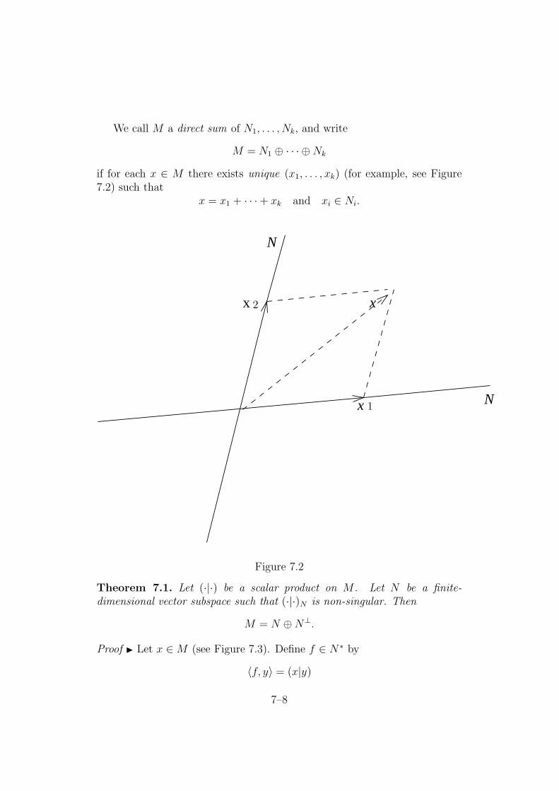
We call M a direct sum of N1, . . . , Nk, and write
M = N1 ⊕ · · · ⊕Nk
if for each x ∈ M there exists unique (x1, . . . , xk) (for example, see Figure7.2) such that
x = x1 + · · ·+ xk and xi ∈ Ni.
x
x
x
N
N
2
1
Figure 7.2
Theorem 7.1. Let (·|·) be a scalar product on M . Let N be a finite-dimensional vector subspace such that (·|·)N is non-singular. Then
M = N ⊕N⊥.
Proof I Let x ∈M (see Figure 7.3). Define f ∈ N ∗ by
〈f, y〉 = (x|y)
7–8

for all y ∈ N .Since (·|·)N is non-singular we can raise the index of f , and get a unique
vector z ∈ N such that〈f, y〉 = (z|y)
for all y ∈ N , i.e.(x|y) = (z|y)
for all y ∈ N , i.e.(x− z|y) = 0
for all y ∈ N , i.e.x− z ∈ N⊥,
y
N
z
xx-z
N
Figure 7.3
i.e.x = z
∈N+ (x− z)
∈N⊥
uniquely, as required. J
Lemma 7.1. Let (·|·) be a symmetric scalar product, not identically zero ona vector space M over a field K of characteristic 6= 2. (i.e. 1+1 6= 0). Thenthere exists x ∈M such that
(x|x) 6= 0.
Proof I Choose x, y ∈M such that (x|y) 6= 0. Then
(x + y|x + y) = (x|x) + (x|y) + (y|x) + (y|y).
Hence (x + y|x + y), (x|x), (y|y) are not all zero. Hence result. J
7–9
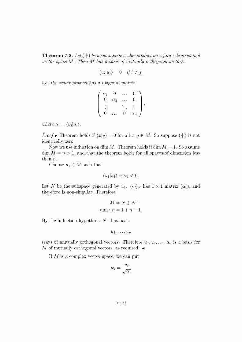
Theorem 7.2. Let (·|·) be a symmetric scalar product on a finite-dimensionalvector space M . Then M has a basis of mutually orthogonal vectors:
(ui|uj) = 0 if i 6= j,
i.e. the scalar product has a diagonal matrix
α1 0 . . . 00 α2 . . . 0...
. . ....
0 . . . 0 αn
,
where αi = (ui|ui).
Proof I Theorem holds if (x|y) = 0 for all x, y ∈ M . So suppose (·|·) is notidentically zero.
Now we use induction on dim M . Theorem holds if dim M = 1. So assumedim M = n > 1, and that the theorem holds for all spaces of dimension lessthan n.
Choose u1 ∈M such that
(u1|u1) = α1 6= 0.
Let N be the subspace generated by u1. (·|·)N has 1 × 1 matrix (α1), andtherefore is non-singular. Therefore
M = N ⊕N⊥
dim : n = 1 + n− 1.
By the induction hypothesis N⊥ has basis
u2, . . . , un
(say) of mutually orthogonal vectors. Therefore u1, u2, . . . , un is a basis forM of mutually orthogonal vectors, as required. J
If M is a complex vector space, we can put
wi =ui√αi
7–10

for each αi > 0. Then (wi|wi) = 1 or 0, and rearranging we have a basis wrtwhich (·|·) has matrix
11
. . .
1
0
0
00
. . .
0
(r × r diagonal block top left), and the associated quadratic form is a sumof squares:
(w1)2 + · · ·+ (wr)2.
If M is a real vector space, we can put
wi =
ui/√
αi αi > 0;
ui/√−αi αi < 0;
ui αi = 0.
Then (wi|wi) = ±1 or 0, and rearranging we have a basis wrt which (·|·) hasmatrix
1. . .
1
0 0
0
−1. . .
−1
0
0 0
0. . .
0
,
and the associated quadratic form is a sum and difference of squares:
(w1)2 + · · ·+ (wr)2 − (wr+1)2 − · · · − (wr+s)2.
7–11

Example: Let (·|·) be a scalar product on a 3-dimensional space M whichhas matrix
A =
4 2 22 0 −12 −1 −3
wrt a basis with coordinate functions x, y, z.To find new coordinate functions wrt which (·|·) has a diagonal matrix.
Method : Take the associated quadratic form
F = 4x2 − 3z2 + 4xy + 4xz − 2yz,
and write it as a sum and difference of squares, by ‘completing squares’. Wehave:
F = 4(x2 + xy + xz)− 3z2 − 2yz
= 4(x + 12y + 1
2z)2 − y2 − z2 − 2yz − 3z2 − 2yz
= 4(x + 12y + 1
2z)2 − (y2 + 4yz + 4z2)
= 4(x + 12y + 1
2z)2 − (y + 2z)2 + 0z2
= 4u2 − v2 + 0w.
Therefore (·|·) has diagonal matrix
D =
4 0 00 −1 00 0 0
wrt to coordinate functions
u = x + 12y + 1
2z,
v = y + 2z,
w = z.
The transition matrix is
P =
1 12
12
0 1 20 0 1
.
Check : P tDP = A?
1 0 012
1 012
2 1
4 0 00 −1 00 0 0
1 12
12
0 1 20 0 1
=
4 2 22 0 −12 −1 −3
.
7–12

For a symmetric scalar product on a real vector space the number of+ signs, and the number of − signs, when the matrix is diagonalised, isindependent of the coordinates chosen:
Theorem 7.3 (Sylvester’s Law of Inertia). Let u1, . . . , un and w1, . . . , wn
be bases for a real vector space, and let
F = (u1)2 + · · ·+ (ur)2 − (ur+1)2 − · · · − (ur+s)2
= (w1)2 + · · ·+ (wt)2 − (wt+1)2 − · · · − (wt+k)2
be a quadratic form diagonalised by each of the two bases. Then r = t ands = k.
Proof I Suppose r 6= t, r > t (say). The space of solutions of the n − r + thomogeneous linear equations
ur+1 = 0, . . . , un = 0, w1 = 0, . . . , wt = 0
has dimension at least
n− (n− r + t) = r − t > 0.
Therefore there exists a non-zero solution x so
F (x) = (u1(x))2 + · · ·+ (ur(x))2 > 0
= −(wt+1(x))2 − · · · − (wt+k(x))2 ≤ 0,
which is clearly a contradiction. Therefore r = t, and similarly s = k. J
7.5 Special Spaces
Definition. A real vector space M with a symmetric scalar product (·|·) iscalled a Euclidean space if the associated quadratic form is positive definite,i.e.
F (x) = (x|x) > 0 for all x 6= 0,
i.e. there exists basis u1, . . . , un such that (·|·) has matrix
1 0 . . . 00 1 . . . 0...
. . ....
0 . . . 0 1
(all + signs).
7–13

F = (u1)2 + · · ·+ (un)2,
(ui|uj) = δij,
i.e. u1, . . . , un is orthonormal.We write
‖x‖ =√
(x|x) (x ∈M),
and call it the norm of x. We have
‖x + y‖ ≤ ‖x‖+ ‖y‖ (Triangle Inequality).
Thus M is a normed vector space, and therefore a metric space, and thereforea toplogical space.
The scalar product also satisfies:
|(x|y)| ≤ ‖x‖‖y‖ (Schwarz Inequality).
We define the angle θ between two non-zero vectors x, y by:
(x|y)
‖x‖‖y‖ = cos θ (0 ≤ θ ≤ π)
(see Figure 7.4).
0
1
-1
π
Figure 7.4
If M is an n-dimensional vector space with scalar product having anorthonormal basis (e.g. a complex vector space or a Euclidean vector space)then the transition matrix P from one orthonormal basis to another satisfies:
P tIPnew
= Iold
,
7–14
i.e.P tP = I
i.e. P is an orthogonal matrix, i.e.
· · · ith col of P · · ·
...jth
colof P
=
1 0 . . . 00 1 . . . 0...
. . ....
0 . . . 0 1
,
i.e.(ith col of P ).(jth col of P ) = δij,
i.e. the columns of P form an orthonormal basis of Kn.Also
P orthonormal⇔ P t = P−1
⇔ PP t = I
⇔ the rows of P form an orthonormal basis of Kn.
Definition. A real 4-dimensional vector space M with scalar product (·|·)of type + + +− is called a Minkowski space. A basis u1, u2, u3, u4 is called aLorentz basis if wrt ui the scalar product has matrix
1 0 0 00 1 0 00 0 1 00 0 0 −1
,
i.e.F = (u1)2 + (u2)2 + (u3)2 − (u4)2.
The transition matrix P from one Lorentz basis to another satisfies:
P t
1 0 0 00 1 0 00 0 1 00 0 0 −1
P =
1 0 0 00 1 0 00 0 1 00 0 0 −1
.
Such a matrix P is called a Lorentz matrix.
Example: On Cn we define the hermitian dot product (x|y) of vectors
x = (α1, . . . , αn), y = (β1, . . . , βn)
7–15

to be(x|y) = α1β1 + · · ·+ αnβn.
This has the property of being positive definite, since:
(x|x) = α1α1 + · · ·+ αnαn = ‖α1‖2 + · · ·+ ‖αn‖2 > 0 if x 6= 0.
More generally:
Definition. If M is a complex vector space then a hermitian scalar product(·|·) on M is a function
M ×M → C
such that
(i) (x + y|z) = (x|z) + (y|z),
(ii) (αx|z) = α(x|z),
(iii) (x|y + z) = (x|y) + (x|z),
(iv) (x|αy) = α(x|y),
(v) (x|y) = (y|x).
(i) and (ii) imply linear in the first variable, (iii) and (iv) imply conjugate-linear in the second variable, (v) implies conjugate-symmetric.
If, in addition,(x|x) > 0
for all x 6= 0 then we call (·|·) a positive definite hermitian scalar product.
Definition. A complex vector space M with a positive definite hermitianscalar product (·|·) is called a Hilbert space.
Note. For a finite dimensional complex space M with an hermitian form (·|·)we can prove (in exactly the same way as for a real space with symmetricscalar product):
7–16

1. There exists basis wrt which (·|·) has matrix
1. . .
1
0 0
0
−1. . .
−1
0
0 0
0. . .
0
.
2. The number of + signs and the number of − signs are each uniquelydetermined by (·|·).
3. M is a Hilbert space iff all the signs are +.
Thus M is a Hilbert space iff M has an orthonormal basis. The transitionmatrix P from one orthonormal basis to another satisfies:
P tIPnew
= Iold
,
i.e.P tP = I.
Such a matrix is called a unitary matrix.
A Hilbert space M is a normed space, hence a metric space, hence atopological space if we define:
‖x‖ =√
(x|x).
To test how many +,− signs a quadratic form has we can use determi-nants:
Example:
F = ax2 + 2bxy + cy2 = a
(
x +b
ay
)2
+ac− b2
ay2
7–17

on a 2-dimensional space, with coordinate functions x, y and matrix
(a bb c
)
.
Therefore
++ ⇔ a > 0,
∣∣∣∣
a bb c
∣∣∣∣> 0,
−− ⇔ a < 0,
∣∣∣∣
a bb c
∣∣∣∣> 0,
+− ⇔∣∣∣∣
a bb c
∣∣∣∣< 0.
More generally:
Theorem 7.4 (Jacobi’s Theorem). Let F be a quadratic form on a realvector space M , with symmetric matrix gij wrt basis ui. Suppose each of thedeterminants
∆i =
∣∣∣∣∣∣∣
g11 . . . g1i
......
gi1 . . . gii
∣∣∣∣∣∣∣
is non-zero (i = 1, . . . , n). Then there exists a basis wi such that F hasmatrix
1∆1
∆1
∆2
. . .∆n−1
∆n
,
i.e.
F =1
∆1(w1)2 +
∆1
∆2(w2)2 + · · ·+ ∆n−1
∆n
(wn)2.
Thus
F is +ve definite⇔ ∆1, ∆2, . . . , ∆n all positive,
F is −ve definite⇔ ∆1 < 0, ∆2 > 0, ∆3 < 0, . . . .
Proof I F (x) = (x|x), where (·|·) is a symmetric scalar product, (ui|uj) = gij.Let
Ni = S(u1, . . . , ui).
(·|·)Niis non-singular, since ∆i 6= 0 for i = 1, . . . , n.
Now
0 ⊂ N1 ⊂ N2 ⊂ · · · ⊂ Ni−1 ⊂ Ni ⊂ · · · ⊂ Nn = M.
7–18

Therefore
Ni = Ni−1 ⊕ (Ni ∩N⊥i−1)
dim : i = (i− 1) + 1.
Choose non-zero wi ∈ Ni ∩N⊥i−1. Then
w1, . . . , wi−1, wi, . . . , wn
are mutually orthogonal, and wi is orthogonal to u1, . . . , ui−1. Therefore wi
is not orthogonal to ui, since (·|·) is non-singular. Therefore we can choosewi such that (ui|wi) = 1.
It remains to show that
(wi|wi) =∆i−1
∆i
.
To do this we write
λ1u1 + · · ·+ λi−1ui−1 + λiui = wi.
Taking scalar product with wi, u1, u2, . . . , ui we get:
0 + · · ·+ 0 + λi = (wi|wi)
λ1g11 + · · ·+ λi−1g1,i−1 + λig1i = 0
λ1g21 + · · ·+ λi−1g2,i−1 + λig2i = 0
...
λ1gi−1,1 + · · ·+ λi−1gi−1,i−1 + λigi−1,i = 0
λ1gi1 + · · ·+ λi−1gi,i−1 + λigii = 1
Therefore
(wi|wi) = λi =
∣∣∣∣∣∣∣∣∣
g11 . . . g1,i−1 0...
......
gi−1,1 . . . gi−1,i−1 0gi1 . . . gi,i−1 1
∣∣∣∣∣∣∣∣∣
∣∣∣∣∣∣∣∣∣
g11 . . . g1,i−1 g1i
......
...gi−1,1 . . . gi−1,i−1 gi−1,i
gi1 . . . gi,i−1 gii
∣∣∣∣∣∣∣∣∣
=∆i−1
∆i
,
as requried. J
This has an application in Calculus:
7–19

Theorem 7.5 (Criteria for local maxima or minima). Let f be a scalarfield on a manifold X such that dfX = 0, and let yi be coordinates on X ata. Put
∆i =
∣∣∣∣∣∣∣∣
∂2f
∂y12 . . . ∂2f
∂y1∂yi
......
∂2f
∂yi∂y1 . . . ∂2
∂yi2
∣∣∣∣∣∣∣∣
.
Then
1. If ∆i(a) > 0 for i = 1, . . . , n then there exists open nbd V of a suchthat
f(x) > f(a) for all x ∈ V, x 6= a,
i.e. a is a local minima of f ;
2. If ∆1(a) < 0, ∆2(a) > 0, ∆3(a) < 0, . . . then there exists open nbd V ofa such that
f(x) < f(a) for all x ∈ V, x 6= a,
i.e. a is a local maxima of f .
To make sure that ‖x‖ =√
(x|x) is a norm on a Euclidean or a Hilbertspace we need to show that the triangle inequality holds.
Theorem 7.6. Let M be a Euclidean or a Hilbert space. Then
(i) |(x|y)| ≤ ‖x‖‖y‖ Schwarz,
(ii) ‖x + y‖ ≤ ‖x‖+ ‖y‖ Triangle.
Proof I
(i) Let x, y ∈M . Then
(x|y) = |(x|y)|eiθ, (y|x) = |(x|y)|e−iθ
(say). So for all λ ∈ R we have:
0 ≤ (λe−iθx + y|λe−iθx + y)
= ‖x‖2λ2 + λe−iθ(x|y) + λeiθ(y|x) + ‖y‖2= ‖x‖2 + 2λ|(x|y)|+ ‖y‖2.
Therefore|(x|y)|2 ≤ ‖x‖2‖y‖2 (‘b2 ≤ 4ac,).
Therefore|(x|y)| ≤ ‖x‖‖y‖.
7–20

(ii)
‖x + y‖2 = (x + y|x + y)
= ‖x‖2 + (x|y) + (y|x) + ‖y‖2≤ ‖x‖2 + 2‖x‖‖y‖+ ‖y‖2
= (‖x‖+ ‖y‖)2.
Therefore‖x + y‖ ≤ ‖x‖+ ‖y‖.
J
7–21

Chapter 8
Linear Operators 2
8.1 Adjoints and Isometries
Let M be a finite dimensional vector space with a fixed non-singular sym-metric or hermitian scalar product (·|·). Recall that if
MT→M
is a linear operator then the adjoint of T is the operator
MT ∗
→M,
which satisfies(x|Ty) = (T ∗x|y)
for all x, y ∈M .If (·|·) has matrix G wrt basis ui and T has matrix A then T ∗ has matrix
A∗ = G−1AtG (G−1AtG in hermitian case)
becauseX tGAY = X tGAG−1GY = [G−1AtGX]tGY,
and similarly
X tGAY = X tGAG−1GY = [G−1AtGX]tGY .
8–1

Examples:
1. M Euclidean, basis orthonormal:
A∗ = At.
2. M Hilbert, basis orthonormal:
A∗ = At.
3. M Minkowski, basis Lorentz:
A∗ =
1 0 0 00 1 0 00 0 1 00 0 0 −1
At
1 0 0 00 1 0 00 0 1 00 0 0 −1
.
Definition. An operator MT→M is called an isometry if
(Tx|Ty) = (x|y) for all x, y ∈ M,
i.e. T preserves (·|·), i.e.(T ∗Tx|y) = (x|y),
i.e.T ∗T = 1,
i.e.T ∗ = T−1.
Examples:
1. M Euclidean, basis orthonormal, A matrix of T :
T is an isometry⇔ AtA = I,
i.e. A is an orthogonal matrix.
2. M Hilbert, basis orthonormal, A matrix of T :
T is an isometry⇔ AtA = I,
i.e. A is a unitary matrix.
8–2

3. M Minkowski, basis Lorentz, A matrix of T :
T is an isometry⇔ GAtGA = I ⇔ AtGA = G,
i.e. A is a Lorentz matrix.
Definition. An isometry of a Euclidean space is called an orthogonal trans-formation. An isometry of a Hilbert space is called a unitary transformation.An isometry of a Minkowski space is called a Lorentz transformation.
Definition. An operator MT→M is called self-adjoint if
T ∗ = T,
i.e.(Tx|y) = (x|Ty) for all x, y ∈ M,
i.e.(ui|Tuj) = (Tui|uj) = (uj|Tui),
i.e. covariant components of T are symmetric.
(In quantum mechanics physical quantities are always represented by self-adjoint operators).
Examples:
1. M Euclidean, basis orthonormal, A matrix of T :
T is self-adjoint⇔ At = A,
i.e. A is symmetric.
2. M Hilbert, basis orthonormal, A matrix of T :
T is self-adjoint⇔ At= A,
i.e. A is hermitian.
3. M Minkowski, basis Lorentz, A matrix of T :
T is self-adjoint⇔ GAtG = A.
Summary: Let MT→ M have matrix A wrt orthonormal or Lorentz basis.
Then:
Space: Euclidean Hilbert Minkowski
Matrix of T ∗: At At
GAtG
T self-adjoint: At = A At= A GAtG = A
A symmetric A Hermitian
T an isometry: AtA = I AtA = I AtGA = G
A orthogonal A unitary A Lorentz
8–3
8.2 Eigenvalues and Eigenvectors
Definition. A vector space N ⊂ M is called invariant under a linear oper-
ator MT→M if
T (N) ⊂ N,
i.e. x ∈ N ⇒ Tx ∈ N .A non-zero vector in a 1-dimensional invariant subspace under T is called
an eigenvector of T :
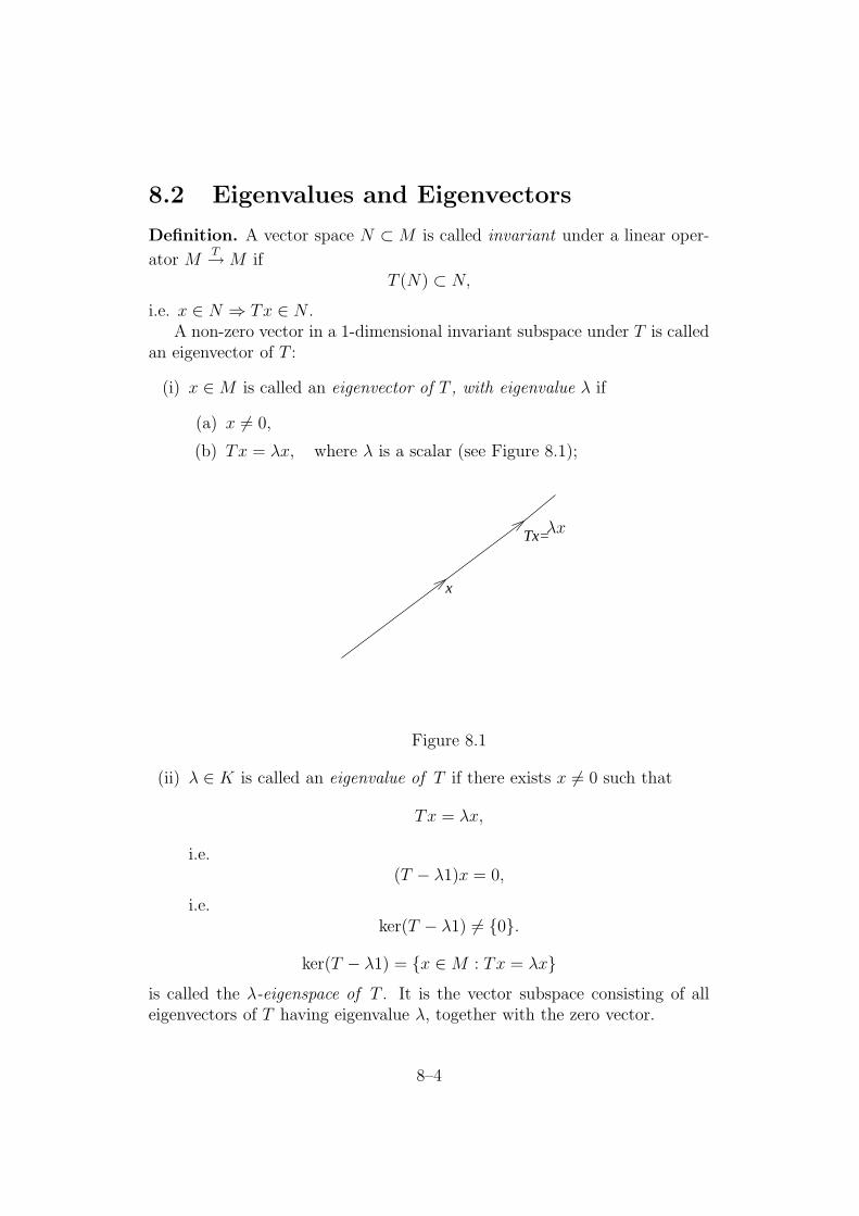
(i) x ∈M is called an eigenvector of T , with eigenvalue λ if
(a) x 6= 0,
(b) Tx = λx, where λ is a scalar (see Figure 8.1);
x
Tx=λx
Figure 8.1
(ii) λ ∈ K is called an eigenvalue of T if there exists x 6= 0 such that
Tx = λx,
i.e.(T − λ1)x = 0,
i.e.ker(T − λ1) 6= 0.
ker(T − λ1) = x ∈M : Tx = λxis called the λ-eigenspace of T . It is the vector subspace consisting of alleigenvectors of T having eigenvalue λ, together with the zero vector.
8–4

Definition. If MT→ M is a linear operator on a vector space of finite di-
mension n, with matrix A =(αi
j
)wrt basis ui, then the polynomial of degree
n with coefficients in K:
char T = det
∣∣∣∣∣∣∣∣∣
α11 −X α1
2 . . . α1n
α21 α2
2 −X...
.... . .
...αn
1 . . . . . . αnn −X
∣∣∣∣∣∣∣∣∣
= det(A−XI)
is called the characteristic polynomial of T .
char T is well-defined, independent of choice of basis ui, since if B is thematrix of T wrt another basis then
B = PAP−1.
Therefore
det(B −XI) = det(PAP−1 −XI)
= det P (A−XI)P−1
= det P det(A−XI) detP−1
= det(A−XI),
since det P det P−1 = det PP−1 = det I = 1.
Theorem 8.1. If MT→M is a linear operator and dim M <∞ and λ ∈ K
thenλ is an eigenvalue of T ⇔ λ is a zero of char T.
Proof I Let T have matrix A wrt basis ui. Then
λ is an eigenvalue of T ⇔ there exists y ∈M such that (T − λ1)y = 0
⇔ there exists Y ∈ Kn such that (A− λI)Y = 0
⇔ det(A− λI) = 0
⇔ λ is a zero of det(A−XI).
J
Corollary 8.1. If T is a linear operator on a finite dimensional complexspace then T has an eigenvalue, and therefore eigenvectors.
8–5

Theorem 8.2. Let MT→ M be a linear operator on a finite dimensional
vector space M . Then T has a diagonal matrix
λ1
. . .
λn
wrt a basis u1, . . . , un iff ui is an eigenvector of T , with eigenvalue λi, fori = 1, . . . , n.
Proof I
Tu1 = λ1u1 + 0u2 + · · ·+ 0un
Tu2 = 0u1 + λ2u2 + · · ·+ 0un
...
Tun = 0u1 + 0u2 + · · ·+ λnun,
hence result. J
Theorem 8.3. Let MT→M ba a self-adjoint operator on a Hilbert space M .
Then all the eigenvalues of T are real.
Proof I Let Tx = λx, x 6= 0, λ ∈ C. Then
λ(x|x) = (λx|x) = (Tx|x) = (x|Tx) = (x|λx) = λ(x|x).
(x|x) 6= 0. Therefore λ = λ. Therefore λ is real. J
Corollary 8.2. Let A ba a hermitian matrix. Then Cn A→ Cn is a self-adjoint operator wrt hermitian dot product. Therefore all the roots of theequation
det(A−XI) = 0
are real.
Corollary 8.3. Let T be a self-adjoint operator on a finite dimensional Eu-clidean space. Then T has an eigenvector.
Proof I Wrt an orthonormal basis T has a real symmetric matrix A:
At= At = A.
Therefore A is hermitian. Therefore det(A−XI) = 0 has real roots. There-fore T has an eigenvalue. Therefore T has eigenvectors. J
8–6

Theorem 8.4. Let N be invariant under a linear operator MT→ M . Then
N⊥ is invariant under T ∗.
Proof I Let x ∈ N⊥. Then for all y ∈ N we have:
(T ∗x|y) = (x|Ty) = 0.
Therefore T ∗x ∈ N⊥. J
Definition. MT→M is a normal operator if
T ∗T = TT ∗,
i.e. T commutes with T ∗.
Examples:
(i) T self-adjoint ⇒ T normal.
(ii) T an isometry ⇒ T normal.
Theorem 8.5. Let S, T be commuting linear operators M →M (ST = TS).Then each eigenspace of S is invariant under T .
Proof I
Sx = λx⇒ S(Tx) = T (Sx) = T (λx) = λ(Tx),
i.e. x ∈ λ-eigenspace of S ⇒ Tx ∈ λ-eigenspace of S. J
8.3 Spectral Theorem and Applications
Theorem 8.6 (Spectral theorem). Let MT→ M be either a self-adjoint
operator on a finite dimensional Euclidean space or a normal operator ona finite dimensional Hilbert space. Then M has an orthonormal basis ofeigenvectors of T .
Proof I (By induction on dim M). True for dim M = 1. Let dim M = n,and assume the theorem holds for spaces of dimension ≤ n− 1.
Let λ be an eigenvalue of T, Mλ the λ-eigenspace. (·|·)Mλis non-singular,
since (·|·) is positive definite. Therefore
M = Mλ ⊕M⊥
λ .
8–7

Mλ is T -invariant. Therefore M⊥λ is T ∗-invariant. T ∗ commutes with T .
Therefore Mλ is T ∗-invariant. Therefore M⊥λ is T -invariant.
Now(T ∗x|y) = (x|Ty)
for all x, y ∈M⊥λ . Therefore (T ∗)M⊥
λis the adjoint of TM⊥
λ. Therefore
T self-adjoint⇒ TM⊥
λis self-adjoint,
andT normal⇒ TM⊥
λis normal.
But dim M⊥λ ≤ n − 1. Therefore, by induction hypothesis M⊥
λ has anorthonormal basis of eigenvectors of T . Therefore M = Mλ ⊕M⊥
λ has anorthonormal basis of eigenvectors of T . J
Applications:
1. Let A be a real symmetric n× n matrix. Then
(i) Rn has an orthonormal basis of eigenvectors u1, . . . , un of A, witheigenvalues λ1, . . . , λn (say),
(ii) if P is the matrix having u1, . . . , un as rows then P is an orthog-onal matrix and
PAP−1 =
λ1 0 . . . 00 λ2 . . . 0...
. . ....
0 . . . 0 λn
= QtAQ,
where Q = P−1.
Proof I Rn is a Euclidean space wrt the dot product, e1, . . . , en is an
orthonormal basis. Operator RA→ Rn has symmetric matrix A wrt
orthonormal basis e1, . . . , en. Therefore A is self-adjoint. Therefore Rn
has an orthonormal basis u1, . . . , un, with eigenvalues λ1, . . . , λn.
Let P be the transition matrix from orthonormal e1, . . . , en to orthonor-mal u1, . . . , un, with inverse matrix Q. P is an orthogonal matrix, andtherefore
Q = P−1 = P t.
8–8

Q is the transition matrix from ui to ei. Therefore
uj = q1j e1 + · · ·+ qn
j en = (q1j , . . . , q
nj )
= jth column of Q
= jth row of P.
Matrix of operator A wrt basis ui is:
PAP−1 = PAP t =
λ1 0 . . . 00 λ2 . . . 0...
. . ....
0 . . . 0 λn
.
J
2. (Principal axes theorem) Let F be a quadratic form on a finitedimensional Euclidean space M . Then M has an orthonormal basisu1, . . . , un which diagonalises F :
F = λ1(u1)2 + · · ·+ λn(un)2.
Such a basis is called a set of principal axes for F .
Proof I F (x) = B(x, x), where B is a symmetric bilinear form. Raisingan index of B gives a self-adjoint operator T :
(x|Ty) = B(x, y) = (Tx|y).
Let u1, . . . , un be an orthonormal basis of M of eigenvectors of T , witheigenvalues λ1, . . . , λn (say). Then wrt ui the quadratic form F hasmatrix:
B(ui, uj) = (ui|Tuj) = (ui|λjuj) = λjδij,
i.e.
λ1 0 . . . 00 λ2 . . . 0...
. . ....
0 . . . 0 λn
,
as required. J
Note. If F has matrix A = (αij), and (·|·) has matrix G = (gij) thenT has matrix
(αij) = (gikαkj) = G−1A.
8–9

Therefore λ1, . . . , λn are the roots of
det(G−1A−XI) = 0,
i.e.det(A−XG) = 0.
3. Consider the surface
ax2 + by2 + cz2 + 2hxy + 2gxz + 2fyz = k (k > 0)
in R3. The LHS is a quadratic form with matrix
A =
a h gh b fg f c
wrt usual coordinate functions x, y, z. By the principal axes theoremwe can choose new orthonormal coordinates X, Y, Z such that equationbecomes:
λ1X2 + λ2Y
2 + λ3Z2 = k,
where λ1, λ2, λ3 are eigenvalues of A.
The surface is:
an ellipsoid if λ1, λ2, λ3 are all > 0, i.e. if the quadratic form ispositive definite, i.e.
a > 0, ab− h2 > 0, det A > 0 by Jacobi;
a hyperboloid of 1-sheet (see Figure 8.2) if the quadratic form isof type + +− (e.g. X2 + Y 2 = Z2 + 1), i.e.
a > 0, ab− h2 > 0, det A < 0
or a > 0, ab− h2 < 0, det A < 0
or a < 0, ab− h2 < 0, det A < 0;
8–10

Z
Figure 8.2
a hyperboloid of 2-sheets (see Figure 8.3) if the quadratic form isof type +−− (e.g. X2 + Y 2 = Z2 − 1), i.e.
a > 0, ab− h2 < 0, det A > 0
or a < 0, ab− h2 < 0, det A > 0
or a < 0, ab− h2 > 0, det A > 0.
8–11

Z
Figure 8.3
8–12

Chapter 9
Skew-Symmetric Tensors andWedge Product
9.1 Skew-Symmetric Tensors
Definition. A bijective map
σ : 1, 2, . . . , r → 1, 2, . . . , r
is called a permutation of degree r. The group Sr of all permutations ofdegree r is called the symmetric group of degree r. Thus Sr is a group oforder r!.
Let T rM denote the space of all tensors over M of type
M ×M × · · · ×M → K.
Thus T rM consists of all tensors T with components
T (ui1, . . . , uir) = αi1...ir (r lower indices),
T = αi1...irui1 ⊗ · · · ⊗ uir .
ui1 ⊗ · · · ⊗ uir is a basis for T rM .For each σ ∈ Sr, and each T ∈ T rM we define σ.T ∈ T rM by:
(σ.T )(x1, . . . , xr) = T (xσ(1), . . . , xσ(r)).
If T has components αi1...ir then σ.T has components βi1...ir , where
βi1...ir = (σ.T )(ui1 , . . . , uir) = T (uiσ(1), . . . , uiσ(r)
) = αiσ(1). . . αiσ(r)
.
9–1

Theorem 9.1. The group Sr acts on T rM by linear transformations, i.e.
(i) σ.(αT + βS) = α(σ.T ) + β(σ.S),
(ii) σ.(τ.T ) = (στ).T ,
(iii) 1.T = T
for all α, β ∈ K, σ, τ ∈ Sr, S, T ∈ T rM .
Proof I e.g. (ii)
[σ.(τ.T )](x1, . . . , xr) = (τ.T )[xσ(1), . . . , xσ(r)]
= T (xσ(τ(1)), . . . , xσ(τ(r)))
= [(στ).T ](x1, . . . , xr).
Therefore σ.(τ.T ) = (στ).T . J
Note. If σ ∈ Sr, we put
εσ =
+1 if σ is an even permutation;−1 if σ is an odd permutation
= sign of σ.
We have:
(i) εστ = εσετ ,
(ii) ε1 = 1,
(iii) εσ−1= εσ.
Definition. T ∈ T rM is skew-symmetric if
σ.T = εσT for all σ ∈ Sr,
i.e.T (xσ(1), . . . , xσ(r)) = εσT (x1, . . . , xr)
for all σ ∈ Sr, x1, . . . , xr ∈M , i.e. the components αi1...ir of T satisfy:
αiσ(1)...iσ(r)= εσαi1...ir .
Example: T ∈ T 3M , with components αijk is skew-symmetric iff
αijk = −αjik = αjki = −αkji = αkij = −αikj.
It follows that if T is skew-symmetric, with components αi1...ir (from nowon assume K has characteristic zero, i.e. α 6= 0⇒ α + α + · · ·+ α 6= 0) then
9–2

1. αi1...ir = 0 if i1, . . . , ir are not all distinct;
2. if we know αi1...ir for all increasing sequences i1 < · · · < ir then weknow αi1...ir for all sequences i1, . . . , ir;
3. if T is skew-symmetric, with components αi1...ir and S is skew-symmetric,with components βi1...ir , and if αi1...ir = βi1...ir for all increasing se-quences i1 < · · · < ir then T = S.
Theorem 9.2. Let T ∈ T rM . Then∑
σ∈Sr
εσσ.T
is skew-symmetric.
Proof I Let τ ∈ Sr. Then
τ.
(∑
σ∈Sr
εσσ.T
)
= ετ∑
σ∈Sr
ετσ(τσ).T = ετ∑
σ∈Sr
σεσ(σ.T ),
as required. J
Definition. The linear operator
A : T rM → T rM
defined by
AT =1
r!
∑
σ∈Sr
εσσ.T
is called the skew-symmetriser.
Example: Let T ∈ T 3M have components αijk. Then
AT (x, y, z) =
1
6[T (x, y, z)− T (y, x, z) + T (y, z, x)− T (x, z, y) + T (z, x, y)− T (z, y, x)],
and AT has components
βijk =1
6(αijk − αikj + αjki − αjik + αkij − αkji).
9–3

Theorem 9.3. Let S ∈ T sM, T ∈ T tM . Then
(i) A[(AS)⊗ T ] = A[S ⊗ T ] = A[S ⊗AT ],
(ii) A(S ⊗ T ) = (−1)stA(T ⊗ S).
Proof I
(i) We first note that if τ ∈ Ss then
[(τ.S)⊗ T ](x1, . . . , xs, xs+1, . . . , xs+t) = (τ.S)(x1, . . . , xs)T (xs+1, . . . , xs+t)
= S(xτ(1), . . . , xτ(s))T (xs+1, . . . , xs+t)
= S(xτ ′(1), . . . , xτ ′(s))T (xτ ′(s+1), . . . xτ ′(s+t))
= [τ ′.(S ⊗ T )](x1, . . . , xs, xs+1, . . . , xs+t),
where
τ ′ =
(1 . . . s s + 1 . . . s + t
τ(1) . . . τ(s) s + 1 . . . s + t
)
.
Thus(τ.S)⊗ T = τ ′.(S ⊗ T )
and ετ ′
= ετ .
Now
A[(AS)⊗ T ] =1
(s + t)!
∑
σ∈Ss+t
εσσ.
[(
1
s!
∑
τ∈Ss
ετ τ.S
)
⊗ T
]
=1
s!
∑
τ∈Ss
1
(s + t)!
∑
σ∈Ss+t
εστ ′
(στ ′).(S ⊗ T )
=1
s!
∑
τ∈Ss
A(S ⊗ T )
= A(S ⊗ T ).
(ii) Let
τ =
(1 . . . s s + 1 . . . s + t
t + 1 . . . t + s 1 . . . t
)
so that ετ = (−1)st. Then
[τ.(S ⊗ T )](x1, . . . , xs, xs+1, . . . , xs+t) = S ⊗ T [xt+1, . . . , xt+s, x1, . . . , xt]
= T (x1, . . . , xt)S(xt+1, . . . xt+s)
= (T ⊗ S)[x1, . . . , xt+s].
9–4

Thereforeτ.(S ⊗ T ) = T ⊗ S.
Therefore
A(S ⊗ T ) =1
(s + t)!
∑
σ∈Ss+t
εστστ.(T ⊗ S)
= ετ 1
(s + t)!
∑
σ∈Ss+t
εσσ.(T ⊗ S)
= (−1)stA(T ⊗ S),
as required. J
9.2 Wedge Product
Definition. If S ∈ T sM and T ∈ T tM , we define their wedge product (alsocalled exterior product) by
S ∧ T =1
s!t!
∑
σ∈Ss+t
εσσ(S ⊗ T ) =(s + t)!
s!t!A(S ⊗ T ).
Example: Let S, T ∈M ∗ have components αi, βi wrt ui. Then
S ∧ T = S ⊗ T − T ⊗ S.
ThereforeS ∧ T [x, y] = S(x)T (y)− T (x)S(y),
and S ∧ T has components
γij = S ∧ T [ui, uj] = S(ui)T (uj)− T (ui)S(uj) = αiβj − βiαj.
Theorem 9.4. The wedge product has the following properties:
1. (R + S) ∧ T = R ∧ T + S ∧ T ,
2. R ∧ (S + T ) = R ∧ S + R ∧ T ,
3. (λR) ∧ S = λ(R ∧ S) = R ∧ (λS),
4. R ∧ (S ∧ T ) = (R ∧ S) ∧ T ,
9–5

5. S ∧ T = (−1)stT ∧ S,
6. R1 ∧ · · · ∧ Rk = (r1+···+rk)!r1!...rk!
A(R1 ⊗ · · · ⊗ Rk).
(i), (ii) and (iii) imply bilinear; (iv) implies associative; (v) implies gradedcommutative.
Proof I e.g. 4.
(R ∧ S) ∧ T =(r + s + t)!
(r + s)!t!A[(r + s)!
r!s!(A(R⊗ S)⊗ T
]
=(r + s + t)!
r!s!t!A(R⊗ S ⊗ T )
sim.= R ∧ (S ∧ T ).
5.
S ∧ T =(s + t)!
s!t!A(S ⊗ T ) = (−1)st (t + s)!
t!s!A(T ⊗ S) = (−1)stT ∧ S.
6. By induction on k: true for k = 1, assume true for k − 1. Then:
(R1 ∧ · · · ∧ Rk−1) ∧ Rk
=(r1 + · · ·+ rk−1 + rk)!
(r1 + · · ·+ rk−1)!rk!A[r1 + · · ·+ rk−1)!
r1! . . . rk−1!A((R1 ⊗ · · · ⊗ Rk−1)⊗Rk)
]
=(r1 + · · ·+ rk)!
r1! . . . rk!A[R1 ⊗ · · · ⊗Rk].
J
Note. For each integer r > 0 we write
M (r) for the space of all skew-symmetric tensors of type
M × · · · ×M←r→
→ K;
M(r) for the space of all skew-symmetric tensors of type
M∗ × · · · ×M∗
←r→→ K;
M (0) = K = M(0).
9–6

If S ∈M (s) or S ∈ M(s), we say that S has degree s, and we have
S ∧ T = (−1)stT ∧ S if s = deg S, t = deg T.
Thus
1. S ∧ T = T ∧ S if either s or T has even degree;
2. S ∧ T = −T ∧ S if both S and T have odd degree;
3. S ∧ S = 0 if S has odd degree, since S ∧ S = −S ∧ S;
4. T1 ∧ T2 ∧ · · · ∧ S ∧ · · · ∧ S ∧ · · · ∧ Tk = 0 if S has odd degree;
5. If x1, . . . , xr ∈M and i1, . . . , ir are selected from 1, 2, . . . , r then
xi1 ∧ · · · ∧ xir = εi1...irx1 ∧ x2 ∧ · · · ∧ xr,
where
εi1...ir =
1 if i1, . . . , ir is an even permutation of 1, . . . , r;−1 if i1, . . . , ir is an odd permutation of 1, . . . , r;0 otherwise
= εi1...ir
is called a permutation symbol ;
6. If xj = αijyi, (αi
j) = A ∈ Kr×r then
x1 ∧ · · · ∧ xr = (αi11 yi1) ∧ · · · ∧ (αir
r yir)
= αi11 . . . αir
r yi1 ∧ · · · ∧ yir
= εi1...irαi11 . . . αir
r y1 ∧ · · · ∧ yr
= (det A)y1 ∧ · · · ∧ yr.
Theorem 9.5. Let M be n-dimensional, with basis u1, . . . , un. Then
(i) if r > n then M (r) = 0,
(ii) if 1 ≤ r ≤ n then
dim M (r) =n!
r!(n− r)!,
and ui1 ∧ · · · ∧ uiri1<···<ir is a basis for M (r).
Proof I
9–7

(i) If r > n and T ∈M (r) has components αi1...ir then the indices i1, . . . , ircannot be distinct. Therefore T = 0.
(ii) We have
〈ui, uj〉 =
1 i = j;0 i 6= j
= δij.
More generally:
ui1 ∧ · · · ∧ uir [uj1, . . . , ujr]
=∑
σ∈Sr
εσui1 ⊗ · · · ⊗ uir [ujσ(1), . . . , ujσ(r)
]
=∑
σ∈Sr
εσδi1jσ(1)
. . . δirjσ(r)
=
1 if i1, . . . , ir are distinct and an even permutation of j1, . . . , jr;
−1 if i1, . . . , ir are distinct and an odd permutation of j1, . . . , jr;
0 otherwise
= δi1...irj1...jr
(general Kronecker delta).
It follows that if 1 ≤ r ≤ n, and if T ∈ M (r) has components αi1...ir
then the tensor:
(∗)∑
i1<···<ir
αi1...irui1 ∧ · · · ∧ uir
has components
∑
i1<···<ir
αi1...irui1 ∧ · · · ∧ uir [uj1, . . . , ujr
] =∑
i1<···<ir
αi1...irδi1...ir
j1...jr
= αj1...jr,
provided j1 < · · · < jr. Therefore (∗) has the same components as T .Therefore
(∗∗) ui1 ∧ · · · ∧ uiri1<···<ir
generate M (r). Also(∗) = 0⇒ αj1...jr
= 0.
Therefore (∗∗) are linearly independent. Therefore (∗∗) form a basisfor M (r). J
9–8

Chapter 10
Classification of LinearOperators
10.1 Hamilton-Cayley and Primary Decom-
position
Let MT→ M be a linear operator on a vector space M over a field K.
Let K[X] be the ring of polynomials in X with coefficients in K. If p =α0 + α1X + α2X
2 + · · ·+ αrXr, write
p(T ) = α01 + α1T + α2T2 + · · ·+ αrT
r ∈ L(M).
Theorem 10.1 (Hamilton-Cayley). Let T ∈ L(M) have characteristicpolynomial p, and let dim M <∞. Then p(T ) = 0.
Proof I Let T have matrix αij wrt basis ui. Put P = (pi
j), where pij =
αij −Xδi
j. Then P is an n × n matrix of polynomials, and det P = p is thecharacteristic polynomial.
Let qij = (−1)i+j times the determinant of the matrix got from P by
removing the ith column and jth row. Then Q = (qij) is also an n× n matrix
of polynomials, andPQ = (det P )I,
i.e.pi
kqkj = pδi
j
Therefore
p(T )uj = p(T )δijui = pi
k(T )qkj (T )ui
= qkj (T )[αi
k − Tδik]ui = qk
j (T )[αikui − Tuk] = 0
10–1

Therefore p(T ) = 0, as required. J
Example:
(α βγ δ
)
: R2 → R2.
p =
∣∣∣∣
α−X βγ δ −X
∣∣∣∣= X2 − (α + δ)X + αδ − βγ.
Therefore
p
(α βγ δ
)
=
(α βγ δ
)2
− (α + δ)
(α βγ δ
)
+ (αδ − βγ)
(1 00 1
)
=
(0 00 0
)
.
Theorem 10.2 (Primary Decomposition Theorem). Let T ∈ L(M),and let
(T − λ11)r1 . . . (T − λk1)rk = 0,
where λ1, . . . , λk are distinct scalars, and r1, . . . , rk are positive integers.Then
M = M1 ⊕ · · · ⊕Mk,
where Mi = ker(T − λi1)ri for i = 1, . . . , k.
Proof I Let
f = (X − λ1)r1 . . . (X − λk)
rk ,
gi = (X − λi)ri,
f = gihi
(say), so f(T ) = 0 and Mi = ker gi(T ).Now h1, . . . , hk have hcf 1. Therefore there exist
Θ1, . . . , Θk ∈ K[X]
such thatΘ1h1 + · · ·+ Θkhk = 1.
Put Pi = Θi(T )hi(T ). Then
(i) P1 + · · ·+ Pk = 1. Also:
10–2

(ii) for each x ∈M ,
gi(T )Pix = gi(T )Θi(T )hi(T )x = f(T )Θi(T )x = 0.
Therefore Pix ∈Mi,
(iii) if xi ∈Mi and j 6= i then
Pjxi = Θj(T )hj(T )xi = 0,
since gi is a factor of hj, and gi(T )xi = 0.
Thus
1. for each x ∈M we have
x = 1x = P1x + · · ·+ Pkx, Pix ∈Mi;
2. if x = x1 + · · ·+ xk, with xi ∈Mi, then (for example, see Figure 10.1)
xi = (P1 + · · ·+ Pk)xi = Pixi = Pi(x1 + · · ·+ xk) = Pix.
Therefore xi is uniquely determined by x. Therefore
M = M1 ⊕ · · · ⊕Mk,
10–3

x
M
M2
P2x
P1x
1
Figure 10.1
as required. J
Note. Each subspace Mi is invariant under T , since
x ∈M1 ⇒ gi(T )x = 0
⇒ Tgi(T )x = 0
⇒ gi(T )Tx = 0
⇒ Tx ∈Mi.
Therefore, if we take bases for M1, . . . , Mk, and put them together to get abasis for M , then wrt this basis T has matrix
A1 0A2
. . .
0 Ak
,
where Ai is the matrix of TMi, the restriction of T to Mi.
Note also that(TMi
− λi1)ri = 0.
10–4
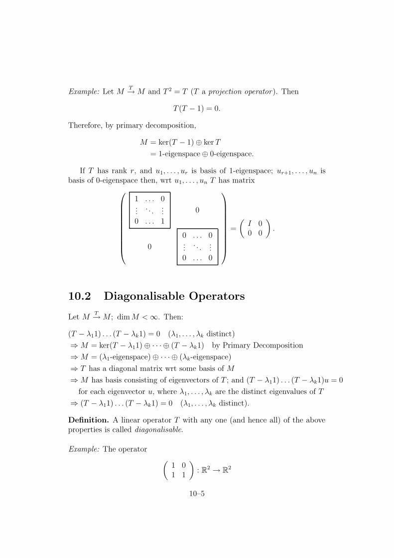
Example: Let MT→M and T 2 = T (T a projection operator). Then
T (T − 1) = 0.
Therefore, by primary decomposition,
M = ker(T − 1)⊕ ker T
= 1-eigenspace⊕ 0-eigenspace.
If T has rank r, and u1, . . . , ur is basis of 1-eigenspace; ur+1, . . . , un isbasis of 0-eigenspace then, wrt u1, . . . , un T has matrix
1 . . . 0...
. . ....
0 . . . 1
0
0
0 . . . 0...
. . ....
0 . . . 0
=
(I 00 0
)
.
10.2 Diagonalisable Operators
Let MT→M ; dim M <∞. Then:
(T − λ11) . . . (T − λk1) = 0 (λ1, . . . , λk distinct)
⇒M = ker(T − λ11)⊕ · · · ⊕ (T − λk1) by Primary Decomposition
⇒M = (λ1-eigenspace)⊕ · · · ⊕ (λk-eigenspace)
⇒ T has a diagonal matrix wrt some basis of M
⇒M has basis consisting of eigenvectors of T ; and (T − λ11) . . . (T − λk1)u = 0
for each eigenvector u, where λ1, . . . , λk are the distinct eigenvalues of T
⇒ (T − λ11) . . . (T − λk1) = 0 (λ1, . . . , λk distinct).
Definition. A linear operator T with any one (and hence all) of the aboveproperties is called diagonalisable.
Example: The operator(
1 01 1
)
: R2 → R2
10–5

is not diagonalisable.
Proof of This B The characteristic polynomial is
∣∣∣∣
1−X 01 1−X
∣∣∣∣= (1−X)2.
Therefore 1 is the only eigenvalue.Also
(α, β) ∈ 1-eigenspace⇔(
1 01 1
)(αβ
)
=
(αβ
)
⇔(
αα + β
)
=
(αβ
)
⇔ α = 0.
Therefore 1-eigenspace = β(0, 1) : β ∈ R is 1-dimensional. Therefore R2
does not have a basis of eigenvectors of
(1 01 1
)
. C
Theorem 10.3. Let S, T ∈ L(M) be diagonalisable (dim M < ∞). Thenthere exists a basis wrt which both S and T have diagonal matrices (S, Tsimultaneously diagonalisable) iff ST = TS (S, T commute).
Proof I
(i) Let M have a basis wrt which S has diagonal matrix
A =
λ1
. . .
λn
and T has diagonal matrix
B =
µ1
. . .
µn
Then AB = BA. Therefore ST = TS.
(ii) Let ST = TS. Since S is diagonalisable we have:
M = M1 ⊕ · · · ⊕Mi ⊕ · · · ⊕Mk,
10–6

distinct sum of eigenspaces of S. Since S and T commute, T leaveseach Mi invariant:
TMi: Mi →Mi.
Since T is diagonalisable we have:
(T − µ11) . . . (T − µl1) = 0,
distinct µ1, . . . , µl. Therefore
(TMi− µ11Mi
) . . . (TMi− µl1Mi
) = 0.
Therefore TMiis diagonalisable. Therefore Mi has a basis of eigenvec-
tors of T . Therefore M has a basis of eigenvectors of S, and of T .J
10.3 Conjugacy Classes
Problem: Given two linear operators
S, T : M →M,
to determine whether they are equivalent up to an isomorphism of M , i.e. is
there a linear isomorphism MR→M so that the diagram
MS−−−→ M
R
y
yR
M −−−→T
M
commutes, i.e.RS = TR,
i.e.RSR−1 = T ?
Definition. S is conjugate to T if there exists a linear isomorphism R suchthat
RSR−1 = T.
Conjugacy is an equivalence relation on L(M); the equivalence classes arecalled conjugacy classes.
10–7

If T ∈ L(M) has matrix A ∈ Kn×n wrt some basis of M then the set ofall matrices which can represent T is:
PAP−1 : P ∈ Kn×n is invertible,which is a conjugacy class in Kn×n.
Conversely, the set of all linear operators on M which can be representedby A is:
RTR−1 : R is a linear isomorphism of M,which is a conjugacy class in L(M).
Hence we have a bijective map from the set of conjugacy classes in L(M)to the set of conjugacy classes in Kn×n (see Figure 10.2).
PAP
TA
RTR −1−1
Figure 10.2
The problem of determining which conjugacy class T belongs to is thusequivalent to determining which conjugacy class A belongs to.
A simple way of distinguishing conjugacy classes is to use properties suchas: rank, trace, determinant, eigenvalues, characteristic polynomial, whichare the same for all elements of a conjugacy class.
Examples:
10–8

1. Let
J =
λ 0 0 01 λ 0 00 1 λ 00 0 1 λ
, a Jordan λ-block of size 4.
(4 × 4, λ on diagonal, 1 just below diagonal, zero elsewhere).
J − λI =
0 0 0 01 0 0 00 1 0 00 0 1 0
.
Therefore
(J − λI)e1 = e2,
(J − λI)e2 = e3,
(J − λI)e3 = e4,
(J − λI)e4 = 0.
ThusK4 e1 e2 e3 e4
↓ ↓ ↓ ↓ ↓im(J − λI) e2 e3 e4 0
↓ ↓ ↓ ↓im(JλI)2 e3 e4 0↓ ↓ ↓
im(j − λI)3 e4 0↓ ↓0 0
Thus
im(J − λI) has basis e2, e3, e4, rank(J − λI) = 3,
im(J − λI)2 has basis e3, e4, rank(J − λI)2 = 2,
im(J − λI)3 has basis e4, rank(J − λI)3 = 1,
(J − λI)4 = 0.
char J =
∣∣∣∣∣∣∣∣
λ−X 0 0 01 λ−X 0 00 1 λ−X 00 0 1 λ−X
∣∣∣∣∣∣∣∣
= (λ−X)4.
Therefore λ is the only eigenvalue of J , and the λ-eigenspace = ker(J−λI) has basis e4.
10–9
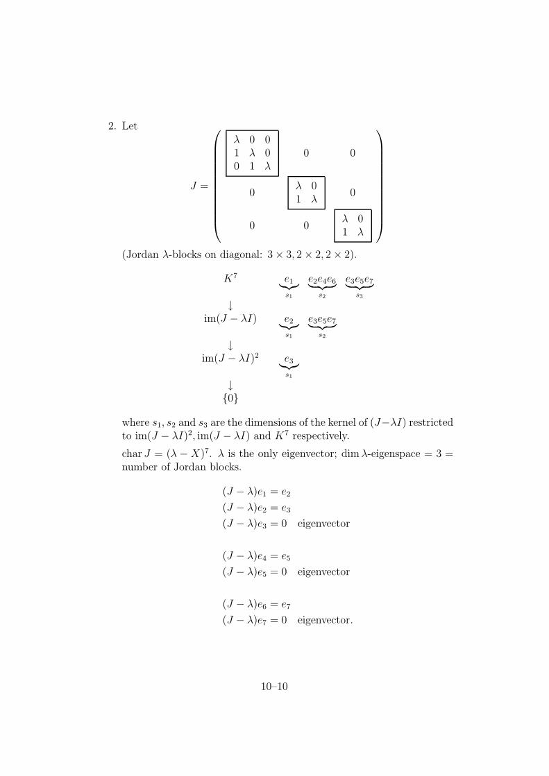
2. Let
J =
λ 0 01 λ 00 1 λ
0 0
0λ 01 λ
0
0 0λ 01 λ
(Jordan λ-blocks on diagonal: 3× 3, 2× 2, 2× 2).
K7 e1︸︷︷︸
s1
e2e4e6︸ ︷︷ ︸
s2
e3e5e7︸ ︷︷ ︸
s3
↓im(J − λI) e2
︸︷︷︸
s1
e3e5e7︸ ︷︷ ︸
s2
↓im(J − λI)2 e3
︸︷︷︸
s1
↓0
where s1, s2 and s3 are the dimensions of the kernel of (J−λI) restrictedto im(J − λI)2, im(J − λI) and K7 respectively.
char J = (λ −X)7. λ is the only eigenvector; dim λ-eigenspace = 3 =number of Jordan blocks.
(J − λ)e1 = e2
(J − λ)e2 = e3
(J − λ)e3 = 0 eigenvector
(J − λ)e4 = e5
(J − λ)e5 = 0 eigenvector
(J − λ)e6 = e7
(J − λ)e7 = 0 eigenvector.
10–10

10.4 Jordan Forms
Definition. A square matrix J ∈ Kn×n is called a Jordan matrix if it is ofthe form
J =
J1
J2
. . .
Jl
,
where each Ji is a Jordan block.
Example:
J =
λ 0 01 λ 00 1 λ
λ 01 λ
µ 01 µ
µ 01 µ
,
(where λ 6= µ (say)) is a 9× 9 Jordan matrix.Note that
(i) char J = (λ−X)5(µ−X)4; eigenvalue λ, with algebraic multiplicity 5;eigenvalue µ, with algebraic multiplicity 4.
(ii)
dimension of λ-eigenspace = number of λ-blocks
= geometric multiplicity of eigenvalue λ = 2;
geometric multiplicity of eigenvalue µ = 2.
10–11

(iii)
J − λI =
0 0 01 0 00 1 0
0 01 0
µ− λ 01 µ− λ
← non-sing.
non-sing. → µ− λ 01 µ− λ
,
(J − λI)2 =
0 0 00 0 01 0 0
0 00 0
(µ− λ)2 01 (µ− λ)2 ← non-sing.
non-sing. → (µ− λ)2 01 (µ− λ)2
,
(J − λ)3 =
0 0 00 0 00 0 0
0 00 0
N.S.
N.S.
.
Therefore
rank(J − λI) = 2 + 1 + 4,
rank(J − λI)2 = 1 + 0 + 4,
rank(J − λI)3 = 0 + 0 + 4.
10–12

More generally, if J is a Jordan n× n matrix, with
b1 λ-blocks of size 1,
b2 λ-blocks of size 2,
...
bk λ-blocks of size k,
and if λ has algebraic multiplicity m then
b1 + 2b2 + 3b3 + · · · = m,
rank(J − λI) has rank:
0b1 + 1b2 + 2b3 + 3b4 + · · ·+ (n−m),
rank(J − λI)2 has rank:
0b1 + 0b2 + 1b3 + 2b4 + · · ·+ (n−m),
rank(J − λI)3 has rank:
0b1 + 0b2 + 0b3 + 1b4 + 2b5 + · · ·+ (n−m),
and so on. Hence the number bk of λ-blocks of size k in J is uniquelydetermined by the conjugacy class of J .
Theorem 10.4. Let T ∈ L(M) be a linear operator on a finite dimensionalvector space over a field K which is algebraically closed. Then T can berepresented by a Jordan matrix J . The matrix J , which by the preceding isuniquely determined, apart from the arrangement of the blocks on the diago-nal, is called the Jordan form of T .
Proof I Since K is algebraically closed, the characteristic polynomial is aproduct of linear factors; so, by Hamilton-Cayley we have
(T − λ11)r1 . . . (T − λk1)rk = 0
(say), with λ1, . . . , λk distinct factors.By primary decomposition:
M = M1 ⊕ · · · ⊕Mk,
10–13

where Mi = ker(T − λi1)ri. We will show that Mi has a basis wrt which TMi
has a Jordan matrix with λi on the diagonal.Put S = TMi
− λi1Mi. Then
MiS→Mi
and Sri = 0, i.e. S is a nilpotent operator. Suppose Sr = 0 but Sr−1 6= 0,and consider:
Mi a1 . . . as1b1 . . . bs2 . . . y1 . . . ysr+1z1 . . . zsr
↓im S↓
im S2
↓...↓
im Sr−3 x1 . . . xs1y1 . . . ys2z1 . . . zs1 . . . zs2 . . . zs3
↓im Sr−2 y1 . . . ys1z1 . . . zs1 . . . zs2
↓im Sr−1 z1 . . . zs1
↓0
(∗)
Choose a basis z1, . . . , zs1 for im Sr−1. Choose y1, . . . , ys1 ∈ im Sr−2 such thatSyj = zj. Extend to a basis z1, . . . , zs1, . . . , zs2 for the kernel of im Sr−2 →im Sr−1. Thus y1, . . . , ys1, z1, . . . , zs2 is a basis for im Sr−2.
Now repeat the construction: choose x1, . . . , xs1 , y1, . . . , ys2 ∈ im Sr−3
such that Sxj = yj, Syi = zi. Extend to a basis z1, . . . , zs2 , . . . , zs3 forthe kernel of im Sr−3 → im Sr−2. Thus x1, . . . , xs1, y1, . . . , ys2, z1, . . . , zs3 is abasis for im Sr−3.
Continue in this way until we get a basis
a1, . . . , as1 , b1, . . . , bs2 , . . . , y1, . . . , ysr−1, z1, . . . , zsr
(say), for Mi, with
Saj = bj, Sbj = cj, . . . , Syj = zj, Szj = 0.
Now write the basis elements in order, by going down each column of (∗)in turn, starting at the left most column (and leaving out any column whoseelements have already been written down).
10–14

Relative to this basis for Mi the matrix of S is a Jordan matrix with zeroson the diagonal. Therefore the matrix of TMi
= S +λi1Miis a Jordan matrix
with λi on the diagonal.Putting together these bases for M1, . . . , Mk we get a basis for M wrt
which T has a Jordan matrix, as required. J
Example: To find a Jordan matrix J conjugate to the matrix
A =
5 4 3−1 0 −31 −2 1
.
The characteristic polynomial is
p =
∣∣∣∣∣∣
5−X 4 3−1 −X −31 −2 1−X
∣∣∣∣∣∣
= (5−X)[−X(1−X)− 6]− 4[−(1−X) + 3] + 3[2 + X]
= (5−X)[X2 −X − 6]− 4[X + 2] + 3[2 + X]
= 5X2 − 5X − 30−X3 + X2 + 6X − 4X − 8 + 3X + 6
= −X3 + 6X2 − 32
= (X + 2)(−X2 + 8X − 16)
= −(X + 2)(X − 4)2.
Therefore, by Hamilton-Cayley the operator R3 A→ R3 satisfies:
(A + 2I)(A− 4I)2 = 0.
Therefore, by primary decomposition:
R3 = ker(A + 2I)⊕ ker(A− 4I)2.
Now
ker(A + 2I) = ker
7 4 3−1 2 −31 −2 3
= ker
7 4 30 18 −180 0 0
row 3 + row 2
7 row 2 + row 1
10–15

Therefore
(α, β, γ) ∈ ker(A + 2I)⇔ 7α + 4β + 3γ = 0
β − γ = 0
⇔ 7α + 7γ = 0
β − γ = 0
⇔ (α, β, γ) = (α,−α,−α) = α(1,−1,−1).
Therefore ker(A + 2I) has basis u1 = (1,−1,−1).
ker(A− 4I)2 = ker
1 4 3−1 −4 −31 −2 −3
2
= ker
0 −18 −180 18 180 18 18
= ker
0 1 10 0 00 0 0
Therefore
(α, β, γ) ∈ ker(A− 4I)2 ⇔ β + γ = 0
⇔ (α, β, γ) = (α, β,−β) = α(1, 0, 0) + β(0, 1,−1).
Therefore (1, 0, 0), (0, 1,−1) is a basis for ker(A− 4I)2.Put
u2 = (1, 0, 0), u3 = (A− 4I)u2 = (1,−1, 1).
So u1, u2, u3 is a basis for R3 such that
(A + 2I)u1 = 0,
(A− 4I)u2 = u3,
(A− 4I)u3 = 0,
i.e.
Au1 = −2u1,
Au2 = 4u2 + u3,
Au3 = 4u3.
10–16

Therefore wrt basis
u1 = (1,−1,−1) = e1 − e2 − e3,
u2 = (1, 0, 0) = e1,
u3 = (1,−1, 1) = e1 − e2 + e3
the operator A has matrix
J =
−2 0 00 4 00 1 4
Let P be the transition matrix from (e1, e2, e3) to (u1, u2, u3).
P =
1 1 1−1 0 −1−1 0 1
−1
=1
2
0 −1 −12 2 00 −1 1
=
0 −12−1
2
1 1 00 −1
2−1
2
.
Therefore
PAP−1 =
0 −12−1
2
1 1 00 −1
212
5 4 3−1 0 −31 −2 1
1 1 1−1 0 −1−1 0 1
=
0 1 14 4 01 −1 2
1 1 1−1 0 −1−1 0 1
=
−2 0 00 4 00 1 4
= J,
as required.
Note. (i)
u1 = e1 − e2 − e3
u2 = e1
u3 = e1 − e2 + e3
⇒
e1 = u2
u1 + u3 = 2e1 − 2e2
u1 − u3 = −2e3
⇒e1 = u2
e2 = −12u1 + u2 − 1
2u3
e3 = −12u1 + 1
2u3
⇒ P =
0 −12−1
2
1 1 00 −1
212
.
10–17

(ii)
1 1 1 1 0 0−1 0 −1 0 1 0−1 0 1 0 0 1
∼
1 1 1 1 0 00 1 0 1 1 00 1 2 1 0 1
∼
1 1 1 1 0 00 1 0 1 1 00 0 2 0 −1 1
∼
2 2 0 2 1 −10 1 0 1 1 00 0 2 0 −1 1
∼
2 0 0 0 −1 −10 1 0 1 1 00 0 2 0 −1 1
Example: To find the Jordan form of
A =
1 1 35 2 6−2 −1 −3
.
char A =
∣∣∣∣∣∣
1−X 1 35 2−X 6−2 −1 −3−X
∣∣∣∣∣∣
= (1−X)[(2−X)(−3−X) + 6]− [5(−3−X) + 12] + 3[−5 + 2(2−X)]
= (1−X)[X2 + X]− [−5X − 3] + 3[−1− 2X]
= X2 + X −X3 −X2 + 5X + 3− 6X − 3
= −X3.
Therefore operator R3 A→ R3 satisfies
A3 = 0.
Now
A2 =
1 1 35 2 6−2 −1 −3
1 1 35 2 6−2 −1 −3
=
0 0 03 3 9−1 −1 −3
.
So put
u1 = e1 = (1, 0, 0) = e1,
u2 = Ae1 = (1, 5,−2) = e1 + 5e2 − 2e3,
u3 = A2e1 = (0, 3,−1) = 3e2 − e3.
So wrt new basis u1, u2, u3 operator A has matrix
J =
0 0 01 0 00 1 0
.
10–18

Alsou2 − 2u3 = e1 − e2.
So
e2 = u1 − u2 + 2u3,
e3 = 3e2 − u3 = 3u1 − 3u2 + 5u3.
Thus
e1 = u1,
e2 = u1 − u2 + 2u3,
e3 = 3u1 − 3u2 + 5u3.
Therefore PAP−1 = J , where
P =
1 1 30 −1 −30 2 5
.
Check:
PA = JP ⇔
1 1 30 −1 −30 2 5
1 1 35 2 6−2 −1 −3
=
0 0 01 0 00 1 0
1 1 30 −1 −30 2 5
⇔
0 0 01 1 30 −1 −3
=
0 0 01 1 30 −1 −3
.
10.5 Determinants
Let M be a vector space of finite dimension n, and MT→ N be a linear
operator. The pull-back (or transpose) of T is the operator
M∗ T ∗
← N∗
defined by〈T ∗f, x〉 = 〈f, Tx〉.
The transpose of T ∗ is T itself (by duality) written T∗. So:
MT∗→ N (T∗ = T ),
M∗ T ∗
← N∗,
〈T ∗f, x〉 = 〈f, T∗x〉.
10–19

If M = N and T has matrix A = (αij) wrt basis ui then
〈T ∗uj, ui〉 = 〈uj, T∗ui〉 = 〈uj, αki uk〉 = αj
i .
Therefore T ∗ has matrix At wrt basis ui.More generally we have the pull-back
M (r) T ∗
← N (r),
and push-forward
M(r)T∗→ N(r)
defined by
(T ∗S)(x1, . . . , xr) = S(T∗x1, . . . , T∗xr),
(T∗S)(f 1, . . . , f r) = S(T ∗f 1, . . . , T ∗f r).
These maps T ∗, T∗ are linear, and preserve the wedge-product. In particular
the spaces M (n) and M(n) are 1-dimensional. Therefore for MT→ M the
push-forward:
M(n)T∗→M(n),
and the pull-back
M (n) T ∗
←M (n)
must each be multiplication by a scalar (called det T, det T ∗ respectively).To see what these scalars are let T have matrix A = (αi
j) wrt basis ui.Then
T∗(u1 ∧ · · · ∧ un) = Tu1 ∧ · · · ∧ Tun
= (αi11 ui1) ∧ · · · ∧ (αin
n uin)
= det A u1 ∧ · · · ∧ un.
Therefore M(n)T∗→M(n) is multiplication by det A. Similarly M (n) T ∗
←M (n) ismultiplication by det At = det A. Therefore
det T = det T ∗ = det A,
independent of choice of basis.
Example: Let dim M = 4, and MT→ M have matrix A = (αi
j) wrt basis ui.Then
dim M(2) =4!
2!2!= 6,
10–20

and wrt basis u1 ∧ u2, u1 ∧ u3, u1 ∧ u4, u2 ∧ u3, u2 ∧ u4, u3 ∧ u4
T∗ : M(2) →M(2)
satisfies
T∗(u1 ∧ u2) = Tu1 ∧ Tu2
= (α11u1 + α2
1u2 + α31u3 + α4
1u4) ∧ (α12u1 + α2
2u2 + α32u3 + α4
2u4)
= (α11α
22 − α2
1α12)u1 ∧ u2 + . . . .
Therefore matrix of T∗ is a 6× 6 matrix whose entries are 2× 2 subdetermi-nants of A.
Theorem 10.5. If MT→M has rank r then
(i) M(r)T∗→M(r) is non-zero,
(ii) M(r+1)T∗→M(r+1) is zero.
Proof I
(i) Let y1, . . . , yr be a basis for im T , and let yi = Txi. Then
T∗ x1 ∧ · · · ∧ xr = Tx1 ∧ · · · ∧ Txr = y1 ∧ · · · ∧ yr 6= 0.
(ii) Let ui be a basis for M . Then
T∗ ui1 ∧ · · · ∧ uir+1 = Tui1 ∧ · · · ∧ Tuir+1 = 0,
since Tui1, . . . , Tuir+1 ∈ im T , which has dimension r. Therefore lin-early independent. J
Corollary 10.1. If T has matrix A then rank T = r ⇔ all (r + 1) × (r +1) subdeterminants are zero, and there exists at least one non-zero r × rsubdeterminant.
10–21

Chapter 11
Orientation
11.1 Orientation of Vector Spaces
Let M be a finite dimensional real vector space. Let P = (pij) be the transi-
tion matrix from basis u1, . . . , un to basis w1, . . . , wn:
uj = pijwi.
Thenu1 ∧ · · · ∧ un = det P w1 ∧ · · · ∧ wn.
Definition. u1, . . . , un has same orientation as w1, . . . , wn if u1 ∧ · · · ∧ un
is a positive multiple of w1 ∧ · · · ∧ wn, i.e. det P > 0. Otherwise oppositeorientation as, i.e. det P < 0.
‘Same orientation as’ is an equivalence relation on the set of all basesfor M . There are just two equivalence classes. We call M an oriented vec-tor space if one of these classes has been designated as positively orientedbases and the other as negatively oriented bases. We call this choosing anorientation for M .
For Rn we may designate the equivalence class of the usual basis e1, . . . , en
as being positively oriented bases. This is called the usual orientation of Rn.
Example: In R3, with usual orientation. e1, e2, e3 (see Figure 11.1) is posi-tively oriented (by definition).
e2 ∧ e1 ∧ e3 = −e1 ∧ e2 ∧ e3,
e2 ∧ e3 ∧ e1 = e1 ∧ e2 ∧ e3.
11–1
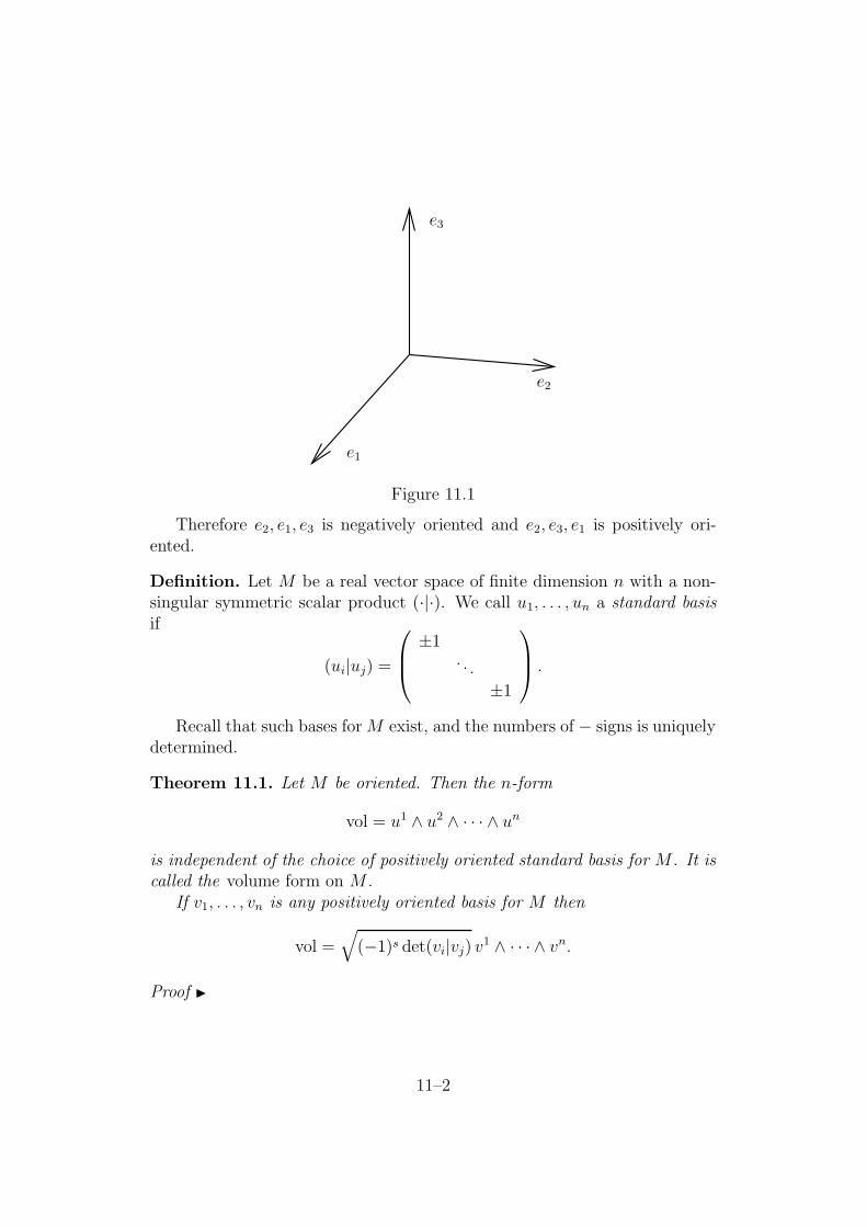
e3
e2
e1
Figure 11.1
Therefore e2, e1, e3 is negatively oriented and e2, e3, e1 is positively ori-ented.
Definition. Let M be a real vector space of finite dimension n with a non-singular symmetric scalar product (·|·). We call u1, . . . , un a standard basisif
(ui|uj) =
±1. . .
±1
.
Recall that such bases for M exist, and the numbers of − signs is uniquelydetermined.
Theorem 11.1. Let M be oriented. Then the n-form
vol = u1 ∧ u2 ∧ · · · ∧ un
is independent of the choice of positively oriented standard basis for M . It iscalled the volume form on M .
If v1, . . . , vn is any positively oriented basis for M then
vol =√
(−1)s det(vi|vj) v1 ∧ · · · ∧ vn.
Proof I
11–2

1. Let w1, . . . , wn be another positively oriented standard basis for M :wi = pi
juj (say). Therefore
w1 ∧ · · · ∧ wn = det P u1 ∧ · · · ∧ un.
But det P > 0 and
P t
±1. . .
±1
P =
±1. . .
±1
.
Therefore(−1)s(det P )2 = (−1)s.
Therefore(det P )2 = 1.
Therefore det P = 1. Therefore
w1 ∧ · · · ∧ wn = u1 ∧ · · · ∧ un = vol,
as required.
2. Let ui = pijv
j (say), det P > 0. Then
P t
±1. . .
±1
P = G,
where gij = (vi|vj). Therefore
(−1)s(det P )2 = det G.
Thereforedet P =
√
(−1)s det G.
Therefore
vol = u1 ∧ · · · ∧ un = det P v1 ∧ · · · ∧ vn =√
(−1)s det Gv1 ∧ · · · ∧ vn,
as required. J
Corollary 11.1. vol has components√| det gij| εi1...in wrt any positively ori-
ented basis.
11–3

Example: Take Rn with usual orientation and dot product. Let
D = t1v1 + · · ·+ tnvn : 0 ≤ ti ≤ 1
be the parallelogram spanned by vectors v1, . . . , vn. Let A be the matrixhaving v1, . . . , vn as columns.
Rn A→ Rn, vi = Aei.
e3
v3 v2e2
v1e1
Figure 11.2
(for example, see Figure 11.2).
vol(v1, . . . , vn) = vol(Ae1, . . . , Aen)
= det A vol(e1, . . . , en)
= det A
= ±| det A|= ±Lebesgue measure of D,
and Lebesgue measure of D =√| det(vi|vj)|.
We continue to consider a real oriented vector space M of finite dimensionn with a non-singular symmetric scalar product (·|·) with s signs.
M (r) denotes the vector space of skew-symmetric tensors of type
M × · · · ×M←r→
→ K.
Theorem 11.2. There exists a unique linear operator
M (r) ∗→M (n−r),
11–4
called the Hodge star operator, with the property that for each positivelyoriented standard basis u1, . . . , un we have
∗(u1 ∧ · · · ∧ ur) = sr+1 . . . snur+1 ∧ · · · ∧ un (no summation here),
where
gij =
s1 0s2
. . .
0 sn
= gij, si = ±1.
Example: If M is 3-dimensional oriented Euclidean, and u1, u2, u3 is anypositively oriented orthonormal then
M (1) ∗→M (2), M (2) →M (1),
with
∗(α1u1 + α2u
2 + α3u3) = α1 u2 ∧ u3 + α2 u3 ∧ u1 + α3 u1 ∧ u2,
∗(α1u2 ∧ u3 + α2u
3 ∧ u1 + α3u1 ∧ u2) = α1u
1 + α2u2 + α3u
3.
Thus, if v has components αi wrt ui, and w has components βi wrt ui then∗(v∧w) has components εijkαjβk wrt ui for any positively oriented orthonor-mal basis ui.
We write v × w = ∗(v ∧ w), and call it the vector product of v and wbecause:
v × w = ∗(v ∧ w)
= ∗[(α1u1 + α2u
2 + α3u3) ∧ (β1u
1 + β2u2 + β3u
3)]
= ∗[(α2β3 − α3β2)u2 ∧ u3 + . . . ]
= (α2β3 − α3β2)u1 + . . . ,
as required.
Proof I(of theorem) If ∗ exists then it must be unique, from the definition.Thus it is sufficient to define one such operator ∗. For any positively orientedbasis we define ∗ω by contraction as:
(∗ω)ir+1...in =(−1)s
r!gi1j1 . . . girjr ωj1...jr
︸ ︷︷ ︸
ω
√
| det gij| εi1...irir+1...in︸ ︷︷ ︸
vol
.
11–5

∗ω is then well-defined independent of choice of basis, since contraction isindependent of a choice of basis. Thus wrt a positively oriented standardbasis u1, . . . , un,
gij =
si i = j0 i 6= j
and ω = u1 ∧ · · · ∧ ur.
ωi...r = 1, other components of ω by skew-symmetry, otherwise zero. There-fore
(∗ω)r+1,...,n =(−1)s
r!s1s2 . . . srω1...rr!1.1 = sr+1 . . . sn,
as required as other components of ∗ω by skew-symmetry are zero.. J
Theorem 11.3. There is a unique scalar product (·|·) on each M (r) suchthat
ω ∧ η = (∗ω|η) vol
for each ω ∈ M (r), η ∈ M (n−r). The scalar product is non-singular andsymmetric for a standard basis
(u1 ∧ · · · ∧ ur|u1 ∧ · · · ∧ ur) = (u1|u1) . . . (ur|ur) = ±1,
and u1∧. . . ur is orthogonal to the other basis element of ui1∧· · ·∧uiri1<···<ir .
Proof I Define (·|·) by ω ∧ η = (∗ω|η) vol. Then (·|·) is a bilinear form onM (n−r).
If u1, . . . , un is a positively oriented standard basis for M then
vol = u1 ∧ · · · ∧ ur
︸ ︷︷ ︸
ω
∧ ur+1 ∧ · · · ∧ un
︸ ︷︷ ︸
η
= (sr+1 . . . snur+1 ∧ · · · ∧ un
︸ ︷︷ ︸
∗ω
| ur+1 ∧ · · · ∧ un
︸ ︷︷ ︸
η
) vol .
Therefore
(ur+1 ∧ · · · ∧ un|ur+1 ∧ · · · ∧ un) = sr+1 . . . sn = (ur+1|ur+1) . . . (un|un),
as required. Similarly other scalar products give zero. J
Similarly other scalar products give zero.
Example: If u1, u2, u3 is an orthonormal basis for M then u2∧u3, u3∧u1, u1∧u3
is an orthonormal basis for M (2), since
(u2 ∧ u3|u2 ∧ u3) = (u2|u2)(u3|u3) = 1.1 = 1,
(u2 ∧ u3|u3 ∧ u1) = (u2|u3)(u3|u1) = 0.0 = 0.
11–6
11.2 Orientation of Coordinate Systems
Definition. Let X be an n-dimensional manifold. Two coordinate systemson X: y1, . . . , yn with domain V , and z1, . . . , zn with domain W have thesame orientation if
∂(y1, . . . , yn)
∂(z1, . . . , zn)> 0
on V ∩W . We call X oriented if a family of coordinate systems is given onX whose domains cover X, and such that any two have the same orientation.We then call these coordinate systems positively oriented.
Note. On V ∩W ,
dyi =∂yi
∂zjdzj.
Therefore
dy1 ∧ · · · ∧ dyn = det
(∂yi
∂zj
)
dz1 ∧ · · · ∧ dzn
=∂(y1, . . . , yn)
∂(z1, . . . , zn)dz1 ∧ · · · ∧ dzn.
Therefore for each a ∈ V ∩W, ∂∂y1
a, . . . , ∂
∂yna
has same orientation as ∂∂z1
a, . . . , ∂
∂zna.
Thus each tangent space TaX is an n-dimensional oriented vector space.If X has a metric tensor (·|·) then TaX has a non-singular symmetric
scalar product (·|·)a for each a ∈ X. Therefore we can define a differentialn-form vol on X, called the volume form on X by:
(vol)a = the volume form on TaX.
Also, if ω is a differential r-form on X then we can define a differential(n− r)-form on X, ∗ω, called the Hodge star of ω by
(∗ω)a = ∗(ωa) for each a ∈ X.
If u1, . . . , un are positively oriented vector fields on X with domain V , and
ds2 = ±(u1)2 ± · · · ± (un)2
thenvol = u1 ∧ · · · ∧ un
on V .
11–7

If y1, . . . , yn is a positively oriented coordinate system on X with domainV then
vol =√
| det gij| dy1 ∧ · · · ∧ dyn
on V , where
gij =
(∂
∂yi| ∂
∂yj
)
.
Examples:
1. R2, with usual coordinates: x, y, and polar coordinates: r, θ (see Figure11.3). Take x, y as positively oriented:
x = r cos θ, y = r sin θ.
Therefore
dx ∧ dy = (cos θ dr − r sin θ dθ) ∧ (sin θ dr + r cos θ dθ) = r dr ∧ dθ.
R
∂∂y
∂∂r
∂∂θ
∂∂x
Figure 11.3
r > 0. Therefore r, θ is positively oriented.
area element = dx ∧ dy = r dr ∧ dθ,
ds2 = (dx)2 + (dy)2 = (dr)2 + (r dθ)2.
Therefore
∗dx = dy, ∗ dy = −dx,
∗dr = r dθ, ∗ (r dθ) = −dr.
11–8

2. Unit sphere S2 in R3 : x2 + y2 + z2 = 1. On S2 we have:
x dx + y dy + z dz = 0.
Therefore (wedge with dx):
y dx ∧ dy + z dx ∧ dz = 0.
Thereforedx ∧ dy =
z
ydz ∧ dx.
Therefore the coordinate system x, y on z > 0 has the same orientationas the coordinate system z, x on y > 0.
We orient S2 so that these coordinates are positively oriented. Now
ds2 = (dx)2 + (dy)2 + (dz)2
= (dx)2 + (dy)2 +(
−x
zdx− y
zdy)2
(on z > 0)
=
(
1 +x2
z2
)
(dx)2 + 2xy
z2dx dy +
(
1 +y2
z2
)
(dy)2.
Therefore wrt coordinates x, y,
gij =
(
1 + x2
z2xy
z2
xy
z2 1 + y2
z2
)
.
Therefore
det gij = 1 +x2
z2+
y2
z2=
x2 + y2 + z2
z2=
1
z2.
Therefore
area element =1
|z|dx ∧ dy.
11–9
Chapter 12
Manifolds and (n)-dimensionalVector Analysis
This chapter could be considered a continuation of Chapter 11.
12.1 Gradient
Definition. If f is a scalar field on a manifold X, with non-singular metrictensor (·|·), then we define the gradient of f to be the vector field grad fsuch that
(grad f |v) =< df |v >= vf = rate of change of f along v
for each vector field v.
Thus grad f is raising the index of df .
df =∂f
∂yidyi
has components∂f
∂yi,
and
grad f = gij ∂f
∂yj
∂
∂yi
has components
gij ∂f
∂yj.
Theorem 12.1. If the metric tensor is positive definite then
12–1

(i) grad f is in the direction of fastest increase of f ;
(ii) the rate of change of f in the direction of fastest increase is ‖ grad f‖;
(iii) grad f is orthogonal to the level surfaces of f (see Figure 12.1).
grad f
Figure 12.1
Proof I
(i) The rate of change of f along any unit vector field v has absolute value
|vf | = |(grad f |v)| ≤ ‖ grad f‖‖v‖ = ‖ grad f‖,
by Cauchy-Schwarz.
(ii) For
v =grad f
‖ grad f‖the maximum is attained:
|vf | =∣∣∣∣
(
grad f | grad f
‖ grad f‖
)∣∣∣∣= ‖ grad f‖.
(iii) If v is tangented to the level surface f = c then
(grad f |v) = vf = 0.
J
Definition. If f is a scalar field on a 2n-dimensional manifold X, withcoordinates
xi = (q1 . . . qn p1 . . . pn)
12–2
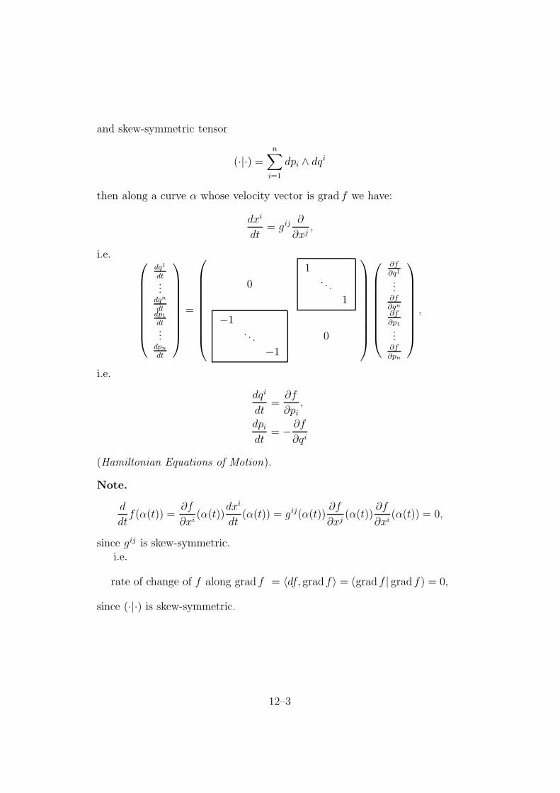
and skew-symmetric tensor
(·|·) =n∑
i=1
dpi ∧ dqi
then along a curve α whose velocity vector is grad f we have:
dxi
dt= gij ∂
∂xj,
i.e.
dq1
dt...
dqn
dtdp1
dt...
dpn
dt
=
0
1. . .
1
−1. . .
−1
0
∂f
∂q1
...∂f
∂qn
∂f
∂p1
...∂f
∂pn
,
i.e.
dqi
dt=
∂f
∂pi
,
dpi
dt= − ∂f
∂qi
(Hamiltonian Equations of Motion).
Note.
d
dtf(α(t)) =
∂f
∂xi(α(t))
dxi
dt(α(t)) = gij(α(t))
∂f
∂xj(α(t))
∂f
∂xi(α(t)) = 0,
since gij is skew-symmetric.i.e.
rate of change of f along grad f = 〈df, grad f〉 = (grad f | grad f) = 0,
since (·|·) is skew-symmetric.
12–3

12.2 3-dimensional Vector Analysis
Given X a 3-dimensional manifold, x, y, z positively oriented orthonormalcoordinates, i.e. metric tensor with line element (dx)2 +(dy)2 +(dz)2. Write
∇ =
(∂
∂x
∂
∂y
∂
∂z
)
, dr = (dx dy dz),
dS = (dy ∧ dz, dz ∧ dx, dx ∧ dy), dV = dx ∧ dy ∧ dz,
F = (F 1 F 2 F 3) = (F1 F2 F3), ∇f =
(∂f
∂x
∂f
∂y
∂f
∂z
)
for a scalar field f,
∇× F =
(∂F 3
∂y− ∂F 2
∂z, ,
)
, ∇.F =∂F 1
∂x+
∂F 2
∂y+
∂F 3
∂z.
The vector field→
F = F.∇ = F 1 ∂
∂x+ F 2 ∂
∂y+ F 3 ∂
∂z
components F , corresponds, lowering the index, to the 1-form (componentsF )
F.dr = F1dx + F2dy + F3dz,
df = (∇f).dr,
d[F.dr] = (∇× F ).dS,
d[F.dS] = (∇.F )dV,
∗1 = dV,
∗dr = dS,
∗dS = dr,
∗V = 1.
Now
1-forms 2-forms 3-froms
Ω(X) → Ω1(X) → Ω2(X) → Ω3(X)
F.drd7→ (∇× F ).dS ∗
f 7→ ∇F.dr F.dSd7→ (∇.F )dV
(∇× F ).dr,~F ,
grad f ,
curl ~F
12–4

12.3 Results
Field Components Typegrad f ∇f vector
curl ~F ∇× F vector
div ~F ∇.F scalar
Theorem 12.2. Let v be a vector field on a manifold, with non-singularsymmetric metric tensor. Let ω be the 1-form given by lowering the index ofv. Then the scalar field divv defined by:
d ∗ ω = (div v) vol
is called the divergence of v. If v has components vi wrt coordinates yi then
div v =1√g
∂
∂yi(√
g vi),
where g = | det gij|.
Proof I
(∗ω)j1...jn−1 = gijvj
√g εij1...jn−1 =
√g viεij1...jn−1.
Therefore
∗ω =√
g v1dy2 ∧ dy3 ∧ · · · ∧ dyn −√g v2dy1 ∧ dy3 ∧ · · · ∧ dyn + . . . .
Therefore
d ∗ ω =∂
∂yi(√
g vi)dy1 ∧ dy2 ∧ · · · ∧ dyn =1√g
∂
∂yi(√
g vi) vol,
as required. J
Theorem 12.3. Let f be a scalar field on a manifold, with non-singularsymmetric metric tensor. Then the scalar field
∆f = div grad f = ∗d ∗ df
is called the Laplacian of f . Wrt coordinates yi we have
∆f =1√g
∂
∂yi
(√g gij ∂f
∂yj
)
.
Thus
∆f =1√g
(∂
∂y1 . . . ∂∂yn
)√g
g11 . . . g1n
......
gn1 . . . gnn
∂f
∂y1
...∂f
∂yn
.
12–5

Examples:
(i) Rn, with (ds)2 = (dx1)2 + · · ·+ (dxn)2, (gij) = I, g = 1. Therefore
∆f =(
∂∂x1 . . . ∂
∂xn
)
∂f
∂x1
...∂
∂xn
=∂2f
∂x12 + · · ·+ ∂2f
∂xn2.
Therefore
∆ =∂2
∂x12 + · · ·+ ∂2
∂xn2usual Laplacian.
(ii) R4, with (ds)2 = (dx)2 + (dy)2 + (dz)2 − (dt)2: Minkowski.
∆f =(
∂∂x
∂∂y
∂∂z
∂∂t
)
11
1−1
∂f
∂x∂f
∂y∂f
∂z∂f
∂t
=∂2f
∂x2+
∂2f
∂y2+
∂2f
∂z2− ∂2f
∂t2.
Therefore
∆ =∂2
∂x2+
∂2
∂y2+
∂2
∂z2− ∂2
∂t2wave operator .
(iii) S2, with (ds)2 = (dθ)2 + (sin θ dϕ)2, gij =
(1 00 sin2 θ
)
, g = sin2 θ.
∆f =1
sin θ
(∂
∂θ
∂
∂ϕ
)
sin θ
(1 00 1
sin2 θ
)( ∂f
∂θ∂f
∂ϕ
)
=1
sin θ
(∂
∂θ
∂
∂ϕ
)(sin θ ∂f
∂θ1
sin θ
∂f
∂ϕ
)
=1
sin θ
[∂
∂θ
(
sin θ∂f
∂θ
)
+∂
∂ϕ
(1
sin θ
∂f
∂ϕ
)]
.
Definition. Let X be a 3-dimensional oriented manifold with non-singularsymmetric metric tensor. Let v be a vector field corresponding to the 1-formω. Then curl v is the vector field corresponding to the 1-form ∗dω. Wrtpositively oriented coordinates yi, curl v has components:
εijk 1√g
(∂vk
∂yj− ∂vj
∂yk
)
,
where g = | det gij|.
12–6

12.4 Closed and Exact Forms
Definition. A differential form ω ∈ Ωr(X) is called
(i) closed if dω = 0;
(ii) exact if ω = dη for some η ∈ Ωr−1(X).
We note that
1. ω exact ⇒ ω closed (d dη = 0),
2. ω an exact 1-form ⇒ ω = df (say)
⇒∫
α
ω =
∫
α
df = 0
for each closed curve α.
Examples:
1. If ω = P dx + Q dy is a 1-form on an open V ⊂ R2 then
ω = dP ∧ dx + dQ ∧ dy
=
(∂P
∂xdx +
∂P
∂ydy
)
∧ dx +
(∂Q
∂xdx +
∂Q
∂ydy
)
∧ dy
=
(∂Q
∂x− ∂P
∂y
)
dx ∧ dy.
Therefore
ω is closed⇔ ∂P
∂y=
∂Q
∂xon V ,
ω is exact⇔ P =∂f
∂x, Q =
∂f
∂y
for some scalar field f on V .
2. The 1-form
ω =x dy − y dx
x2 + y2
on R2 − 0 is called the angle-form about 0. We have:
∂
∂x
(x
x2 + y2
)
= +1
x2 + y2− 2x2
(x2 + y2)2=
y2 − x2
(x2 + y2)2,
∂
∂y
( −y
x2 + y2
)
= − 1
x2 + y2+
2y2
(x2 + y2)2=
y2 − x2
(x2 + y2)2.
12–7

Therefore ω is closed.
ω is not exact because if α(t) = (cos t, sin t) is the unit circle about 0(0 ≤ t ≤ 2π) then
∫
α
ω =
∫ 2π
0
cos t. sin t− sin t.(− sin t)
cos2 t + sin2 tdt =
∫ 2π
0
1 dt = 2π 6= 0.
However, on R2 − negative or zero x-axis we have
x = r cos θ, y = r sin θ,
where θ is a scalar field, with −π ≤ θ ≤ π and
ω =r cos θ.(−r cos θ)− r sin θ.(−r sin θ)
r2 cos2 θ + r2 sin2 θdθ = dθ.
bF
a
Figure 12.2
Therefore, if α is a curve from a to b (see Figure 12.2),
∫
α
ω =
∫
α
dθ = θ(b)− θ(a) = change in angle along α.
Note.
dz
z=
z dz
zz=
(x− iy)(dx + i dy)
x2 + y2=
x dx + y dy
x2 + y2+ i
x dy − y dx
x2 + y2.
Therefore ω = im ∂z∂
.
12–8

3. If~F = F 1 ∂
∂x+ F 2 ∂
∂y+ F 3 ∂
∂z
is a force field in R3 then
F.dr = F1dx + F2dy + F3dz, Fi = F i
is called the work element.∫
α
F.dr = work done by the force ~F along the curve α.
~F is conservative if F.dr is exact, i.e.
F.dr = dV,
where V is a scalar field. V is called a potential function for ~F .
Work done by ~F along α from a to b (see Figure 12.3) is
∫
α
F.dr =
∫
α
dV = V (b)− V (a) = potential difference.
bF
a
α
Figure 12.3
A necessary condition that ~F be conservative is that F.dr be closed,i.e.
∇× F = 0.
12.5 Contraction and Results
Definition. An open set V ⊂ Rn is called contractible to a ∈ V if thereexists a C∞ map
V × [0, 1]ϕ→ V
12–9

such that
ϕ(x, 1) = x,
ϕ(x, 0) = a
for all x ∈ V .
Example: V star-shaped⇒ V contractible. ϕ(x, t) = tx+(1−t)a (see Figure12.4).
x
aφ(x, t)
T
Figure 12.4
Theorem 12.4 (Poincare Lemma). Let ω ∈ Ωr(V ), where V is a con-tractible open subset of Rn, and r ≥ 1. Then ω is exact iff ω is closed.
Proof I Let I = [0, 1] be the unit interval 0 ≤ t ≤ 1, and define a linearoperator (‘homotopy’)
Ωr(V × I)H→ Ωr−1(V )
for each r ≥ 1 by
H[f dt ∧ dxJ ] =
(∫ 1
0
f dt
)
dxJ ,
H[f dxJ ] = 0.
Now calculate the operator dH + Hd:
(i) if η = f dt ∧ dxJ then
dHη + H dη = d
[(∫ 1
0
f dt
)
dxJ
]
+ H
[
− ∂f
∂xidt ∧ dxi ∧ dxJ
]
=
(∫ 1
0
∂f
∂xidt
)
dxi ∧ dxJ −(∫ 1
0
∂f
∂xidt
)
dxi ∧ dxJ
= 0;
12–10
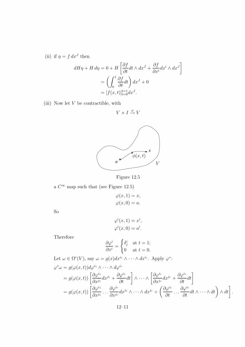
(ii) if η = f dxJ then
dHη + H dη = 0 + H
[∂f
∂tdt ∧ dxJ +
∂f
∂xidxi ∧ dxJ
]
=
(∫ 1
0
∂f
∂tdt
)
dxJ + 0
= [f(x, t)]t=1t=0dxJ .
(iii) Now let V be contractible, with
V × Iϕ→ V
x
aφ(x, t)
V
Figure 12.5
a C∞ map such that (see Figure 12.5)
ϕ(x, 1) = x,
ϕ(x, 0) = a.
So
ϕi(x, 1) = xi,
ϕi(x, 0) = ai.
Therefore∂ϕi
∂xi=
δij at t = 1;
0 at t = 0.
Let ω ∈ Ωr(V ), say ω = g(x)dxi1 ∧ · · · ∧ dxir . Apply ϕ∗:
ϕ∗ω = g(ϕ(x, t))dϕi1 ∧ · · · ∧ dϕir
= g(ϕ(x, t))
[∂ϕi1
∂xj1dxj1 +
∂ϕi1
∂tdt
]
∧ · · · ∧[∂ϕir
∂xjrdxjr +
∂ϕir
∂tdt
]
= g(ϕ(x, t))
[∂ϕi1
∂xj1. . .
∂ϕir
∂xjrdxj1 ∧ · · · ∧ dxjr +
(∂ϕi1
∂t. . .
∂ϕir
∂tdt ∧ · · · ∧ dt
)
∧ dt
]
.
12–11

Apply dH + Hd:
(dH + Hd)ϕ∗ω =
[
g(ϕ(x, t))∂ϕi1
∂xj1. . .
∂ϕir
∂xjr
]t=1
t=0
dxj1 ∧ · · · ∧ dxjr + 0
= g(x)δi1j1
. . . δirjr
dxj1 ∧ · · · ∧ dxjr
= g(x)dxi1 ∧ · · · ∧ dxir
= ω.
Hence:(dH + Hd)ϕ∗ω = ω
for all ω ∈ Ωr(V ).
(iv) Let ω be closed. Then
dϕ∗ω = ϕ∗dω = 0.
ThereforedHϕ∗ω = ω.
Therefore ω is exact. J
Theorem 12.5. Let ω be a closed r-form, with domain V open in manifoldX. Let a ∈ V . Then there exists an open neighbourhood W of a such that ωis exact on W .
Proof I Let y be a coordinate system on X at a, domain U ⊂ V , say. LetW ⊂ U be an open neighbourhood of a such that y(W ) is an open ball (seeFigure 12.8).
y(a)
VUW
y(U)
y(W)
ya
Figure 12.6
12–12

ConsiderW
y→ y(W ), W ←ϕ
y(W )
(open ball), where ϕ is the inverse map.
dϕ∗ω = ϕ∗dω = 0, since ω is closed. Therefore ϕ∗ω is closed. Thereforeϕ∗ω = dη on y(W ), by Poincare. Therefore
dy∗η = y∗dη = y∗ϕ∗ω = ω
on W . Therefore ω is exact on W . J
Theorem 12.6. Let X be a 2-dimensional oriented manifold with a positivedefinite metric tensor. Let u1, u2 be positively oriented orthonormal vectorfields on X, with domain V (moving frame). Then there exists a unique1-form ω on V such that
(∗)(
du1
du2
)
=
(0 −ωω 0
)
∧(
u1
u2
)
on V . ω is called the connection form (gauge field) wrt moving frame u1, u2.
Proof I Any 1-form ω on V can be written uniquely as:
ω = αu1 + βu2, α, β scalar fields.
ω satisfies (∗)⇔ du1 = −ω ∧ u2,
du2 = ω ∧ u1
⇔ du1 = −(αu1 + βu2) ∧ u2 = −αu1 ∧ u2,
du2 = (αu1 + βu2) ∧ u1 = −βu1 ∧ u2.
Thus α, β are uniquely determined. J
Theorem 12.7. Let X be a 2-dimensional oriented manifold with positivedefinite metric tensor. Let u1, u2 be a moving frame with domain V , withconnection form ω and
dω = Ku1 ∧ u2 = K.area element.
Then the scalar field K is independent of the choice of moving frame, and iscalled the Gaussian curvature of X.
12–13

Proof I Let w1, w2 be another moving frame with domain V :
(w1
w2
)
=
(cos θ − sin θsin θ cos θ
)(u1
u2
)
(say). Write this in matrix form as:
w = Pu.
Also (du1
du2
)
=
(0 −ωω 0
)
∧(
u1
u2
)
.
Write this in matrix form as:
du = Ω ∧ u.
Then
dw = (dP ) ∧ u + P du
= (dP ) ∧ u + PΩ ∧ u
= (dP + PΩ) ∧ u
= (dP + PΩ) ∧ P−1w
= [(dP )P−1 + PΩP−1] ∧ w
=
[(− sin θ dθ − cos θ dθcos θ dθ − sin θ dθ
)(cos θ sin θ− sin θ cos θ
)
+
(cos θ − sin θsin θ cos θ
)(0 −ωω 0
)(cos θ sin θ− sin θ cos θ
)]
∧ w
=
[(0 −dθdθ 0
)
+
(0 −ωω 0
)]
∧ w
=
(0 −(ω + dθ)
ω + dθ 0
)
∧ w.
Therefore ω + dθ is the connection form wrt moving frame w1, w2 and
d[ω + dθ] = dω + d dθ = dω,
as required. J
Example: On S2, with angle coordinates θ, ϕ,
ds2 = (dθ)2 + (sin θ dϕ)2, u1 = dθ, u2 = sin θ dϕ.
12–14

Recall
ω = − cos θ dϕ,
dω = sin θ dθ ∧ dϕ = u1 ∧ u2.
Therefore Gaussian curvature is constant function 1.
Theorem 12.8. Let X be an oriented 2-dimensional manifold with positivedefinite metric tensor. Then the Gaussian curvature of X is zero iff for eacha ∈ X there exists local coordinates x, y such that
ds2 = (dx)2 + (dy)2,
i.e.
gij =
(1 00 1
)
.
Proof I Let u1, u2 be a moving frame with connection form ω on an openneighbourhood V of a on which the Poincare lemma holds. Then, on V :
Gaussian curvature is zero⇔ dω = 0
⇔ ω = −dθ (say), by Poincare
⇔ ω + dθ = 0
⇔ u1, u2 can be rotated to a new frame w1, w2
having connection form 0
⇔ dw1 = 0, dw2 = 0
⇔ w1 = dx, w2 = dy (say), by Poincare
⇔ ds2 = (dx)2 + (dy)2.
~N J
12.6 Surface in R3
Let X be a 2-dimensional submanifold of R3. Denote all vectors by theirusual components in R3. Let ~N be a field of unit vectors normal to X, t1, t2
be coordinates on X, and let ~r = (x, y, z). Let ∂~r∂t1
, ∂~r∂t2
be a basis for vectorstangent to X (see Figure 12.9).
∂~r
∂ti. ~N = 0.
12–15
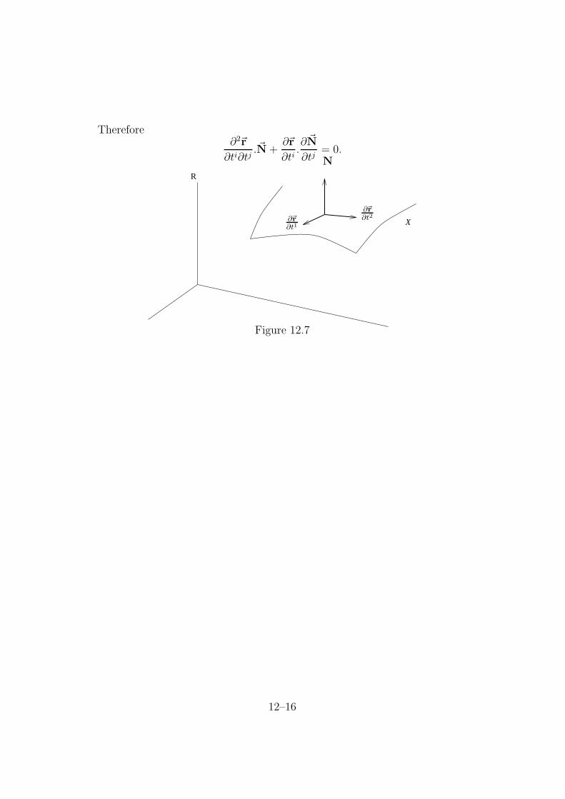
Therefore∂2~r
∂ti∂tj. ~N +
∂~r
∂ti.∂ ~N
∂tj= 0.
R
X
N
∂~r∂t2∂~r
∂t1
Figure 12.7
12–16
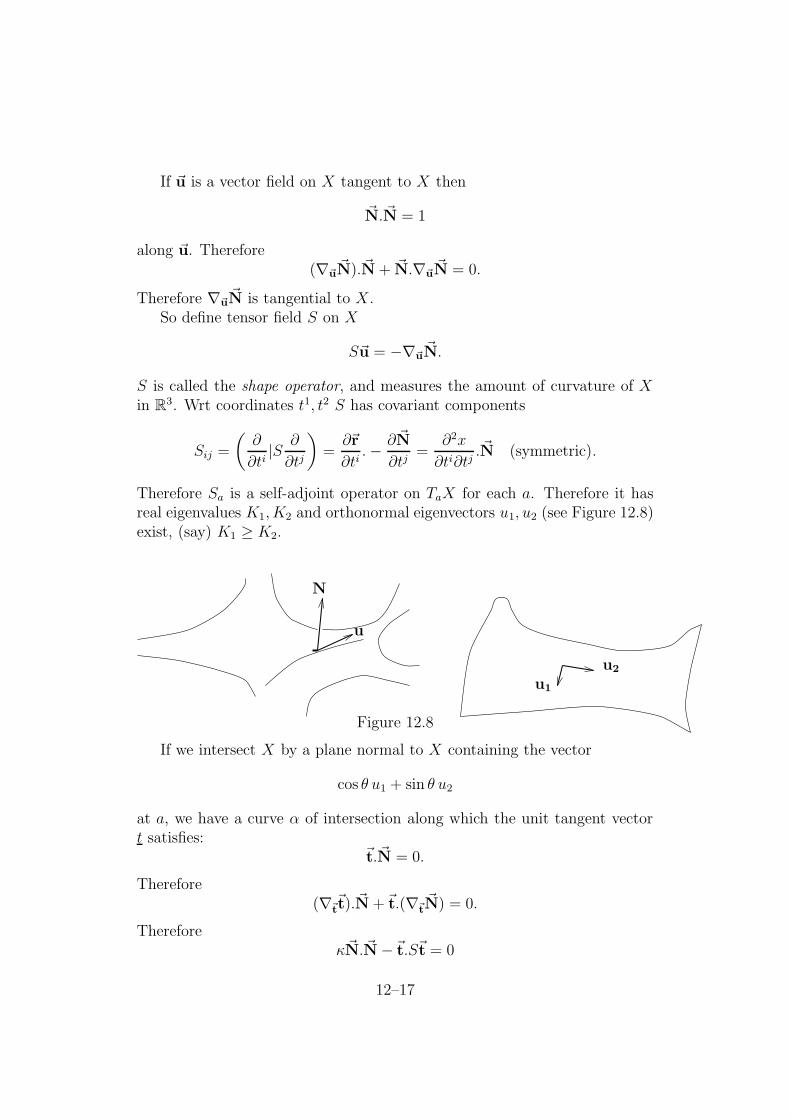
If ~u is a vector field on X tangent to X then
~N. ~N = 1
along ~u. Therefore(∇~u
~N). ~N + ~N.∇~u~N = 0.
Therefore ∇~u~N is tangential to X.
So define tensor field S on X
S~u = −∇~u~N.
S is called the shape operator, and measures the amount of curvature of Xin R3. Wrt coordinates t1, t2 S has covariant components
Sij =
(∂
∂ti|S ∂
∂tj
)
=∂~r
∂ti.− ∂ ~N
∂tj=
∂2x
∂ti∂tj. ~N (symmetric).
Therefore Sa is a self-adjoint operator on TaX for each a. Therefore it hasreal eigenvalues K1, K2 and orthonormal eigenvectors u1, u2 (see Figure 12.8)exist, (say) K1 ≥ K2.
N
u
u2
u1
Figure 12.8
If we intersect X by a plane normal to X containing the vector
cos θ u1 + sin θ u2
at a, we have a curve α of intersection along which the unit tangent vectort satisfies:
~t. ~N = 0.
Therefore(∇~t
~t). ~N +~t.(∇~t~N) = 0.
Thereforeκ~N. ~N−~t.S~t = 0
12–17
at a, where κ is the curvature of α at a. Therefore
κ = ~t.S~t = (cos θ u1 + sin θ u2).S(cos θ u1 + sin θ u2) (at a)
= κ1 cos2 θ + κ2 sin2 θ.
Therefore u1 is the direction of maximum curvature K1, and u2 is the direc-tion of minimum curvature K2.
Put ~N = u3, with u1, u2, u3 a moving frame.
∇u3 = −ω13 ⊗ u1 − ω2
3 ⊗ u2 − ω33 ⊗ u3.
Therefore
Su1 = −∇u1u3 = 〈ω13, u1〉u1 + 〈ω2
3, u1〉u2,
Su2 = −∇u2u3 = 〈ω13, u2〉u1 + 〈ω2
3, u2〉u2.
Therefore
κ1κ2 = det S
= 〈ω13, u1〉〈ω2
3, u2〉 − 〈ω13, u2〉〈ω2
3, u1〉= ω1
3 ∧ ω23(u1, u2)
= dω12(u1, u2)
= κ u1 ∧ u2(u1, u2)
= κ
(since dΩ = −Ω ∧ Ω, so dω12 = −ω1
k ∧ ωk2 = −ω1
3 ∧ ω32 = ω1
3 ∧ ω23).
12.7 Integration on a Manifold (Sketch)
Let ω be a differential n-form on an oriented n-dimensional manifold X. Wewant to define ∫
X
ω,
the integral of ω over X.To justify in detail the construction which follows X must satisfy some
conditions. It is sufficient, for instance, that X be a submanifold of someRN .
(i) Suppose
ω = f(y1, . . . , yn)dy1 ∧ · · · ∧ dyn
= y∗[f(x1, . . . , xn)dx1 ∧ · · · ∧ dxn]
= y∗ω1
12–18
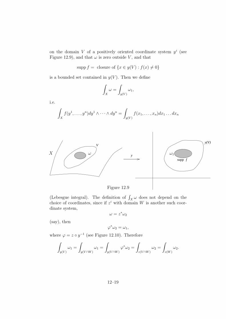
on the domain V of a positively oriented coordinate system yi (seeFigure 12.9), and that ω is zero outside V , and that
supp f = closure of x ∈ y(V ) : f(x) 6= 0
is a bounded set contained in y(V ). Then we define
∫
X
ω =
∫
y(V )
ω1,
i.e.∫
X
f(y1, . . . , yn)dy1 ∧ · · · ∧ dyn =
∫
y(V )
f(x1, . . . , xn)dx1 . . . dxn
fy
y(V)V
supp
X ω ω1
Figure 12.9
(Lebesgue integral). The definition of∫
Xω does not depend on the
choice of coordinates, since if zi with domain W is another such coor-dinate system,
ω = z∗ω2
(say), thenϕ∗ω2 = ω1,
where ϕ = z y−1 (see Figure 12.10). Therefore
∫
y(V )
ω1 =
∫
y(V ∩W )
ω1 =
∫
y(V ∩W )
ϕ∗ω2 =
∫
z(V ∩W )
ω2 =
∫
z(W )
ω2.
12–19

z
V
W
X
y(V) z(W)
y
ω
ω1 ω2
φ
Figure 12.10
(ii) For a general n-form ω on X we write
ω = ω1 + · · ·+ ωr,
where each ωi is an n-form satisfying the conditions of (i), and define
∫
X
ω =
∫
X
ω1 + · · ·+∫
X
ωr,
and check that the result is independent of the choice of ω1, . . . , ωr.
Definition. If X has a metric tensor then
volume of X =
∫
X
volume form.
Example: If
~v = v1 ∂
∂x+ v2 ∂
∂y+ v3 ∂
∂z= ~v.∇
12–20

is a vector field in R3,
v = v1 dx + v2 dy + v3 dz = ~v.d~r
is the corresponding 1-form (vi = vi), and
∗v = v1 dy ∧ dz + v2 dz ∧ dx + v3 dx ∧ dy = ~v.ds
is the corresponding 2-form then if ui is a moving frame, with u3 = ~N normalto surface S (see Figure 12.11), then
~v = αiui,
v = αiui,
∗v = α1 u2 ∧ u3 + α2 u3 ∧ u1 + α3 u1 ∧ u2,
where αi = αi. Therefore pull-back of ∗v to X is
α3u1 ∧ u2 = (~v. ~N)dS,
where dS = u1 ∧ u2 (area form). Therefore∫
v.dS =
∫
(~v. ~N)dS = flux of ~v across S∫
~N.dS =
∫
dS = area of S.
Note. ~v.dr is work element, ~v.ds is flux element, ~N.ds is area element ofvector field ~v.
S
~vu3 = ~N
u1
u2
Figure 12.11
12–21

12.8 Stokes Theorem and Applications
Theorem 12.9 (Stokes). (George Gabriel Stokes 1819 - 1903, Skreen Co.Sligo) Let ω be an (n − 1)-form on an n-dimensional manifold X with an(n− 1)-dimensional boundary ∂X (see Figure 12.12). Then
∫
X
dω =
∫
∂X
i∗ω,
where ∂Xi→ X is the inclusion map.
Proof I(Sketch) We write
ω = ω1 + · · ·+ ωr,
where each ωi satisfies the conditions of either (i), (ii) or (iii) below, and weprove it for each ωi. It then follows for ω.
W
X
V
∂X
Figure 12.12
(i) Letω = f(y1, . . . , yn)dy2 ∧ · · · ∧ dyn
on the domain V of a positively oriented coordinate system yi such that
y(V ) = (−1, 1)× · · · × (−1, 1) (cube),
ω zero outside V , and supp f a closed bounded subset of y(V ) (seeFigure 12.13). ∫
∂X
i∗ω = 0,
since ω is zero on ∂X.
dω =∂f
∂y1dy1 ∧ dy2 ∧ · · · ∧ dyn.
12–22

Therefore∫
X
dω =
∫
y(V )
∂f
∂x1dx1dx2 . . . dxn
=
∫ 1
−1
. . .
∫ 1
−1
[∫ 1
−1
∂f
∂x1dx1
]
dx2 . . . dxn
=
∫ 1
−1
. . .
∫ 1
−1
[f(1, x2, . . . , xn)− f(−1, x2, . . . , xn)]dx2 . . . dxn
= 0.
Therefore ∫
X
dω = 0 =
∫
∂X
i∗ω.
For (ii) and (iii), let ω be zero outside the domain W of functionsy1, y2, . . . , yn, with y a homeomorphism:
y(W ) = (−1, 0]× (−1, 1)× · · · × (−1, 1)
f
y(V)
supp
12–23
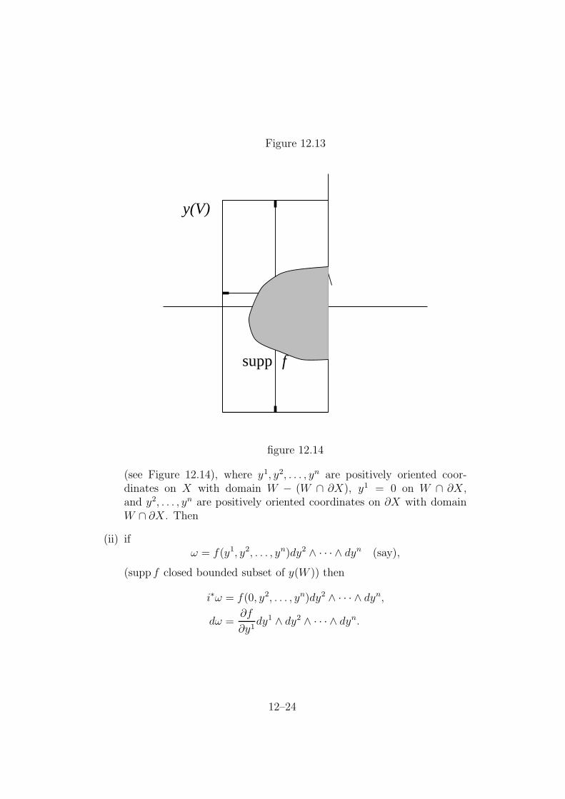
Figure 12.13
f
y(V)
supp
figure 12.14
(see Figure 12.14), where y1, y2, . . . , yn are positively oriented coor-dinates on X with domain W − (W ∩ ∂X), y1 = 0 on W ∩ ∂X,and y2, . . . , yn are positively oriented coordinates on ∂X with domainW ∩ ∂X. Then
(ii) ifω = f(y1, y2, . . . , yn)dy2 ∧ · · · ∧ dyn (say),
(supp f closed bounded subset of y(W )) then
i∗ω = f(0, y2, . . . , yn)dy2 ∧ · · · ∧ dyn,
dω =∂f
∂y1dy1 ∧ dy2 ∧ · · · ∧ dyn.
12–24

Therefore∫
X
dω =
∫
y(W )
∂f
∂x1dx1dx2 . . . dxn
=
∫
y(W∧∂X)
f(0, x2, . . . , xn)dx2 . . . dxn
=
∫
∂X
i∗ω;
(iii) ifω = f(y1, . . . , yn)dy1 ∧ dy3 ∧ · · · ∧ dyn
(say), (supp f closed bounded subset of y(W )) then
i∗ω = 0,
since y1 = 0 on W ∧ ∂X. Also
dω = − ∂f
∂y2dy1 ∧ dy2 ∧ · · · ∧ dyn.
Therefore∫
X
dω = −∫ 1
−1
. . .
∫ 0
−1
[∫ 1
−1
∂f
∂x2dx2
]
︸ ︷︷ ︸
0
dx1 . . . dxn = 0.
Therefore ∫
X
dω = 0 =
∫
∂X
i∗ω.
J
12–25

Applications of Stokes Theorem:
1. In R2: ω 1-form (see Figure 12.17).∫
∂D
i∗ω =
∫
ω
dω,
∫
∂D
(P dx + Q dy) =
∫
D
(∂Q
∂x− ∂P
∂y
)
dx ∧ dy Green’s Theorem.
In particular:
(a)∫
∂D
x dy = −∫
∂D
y dx =1
2i
∫
∂D
z dz =
∫
D
dx ∧ dy = area of D.
(b) if f = u + iv, ω = f dz then
dω =
[
−∂u
∂y− ∂v
∂x+ i
(∂u
∂x− ∂v
∂y
)]
dx ∧ dy.
Nowdω = 0⇔ f holomorphic ,
by Cauchy-Riemann. Therefore∫
∂D
f(z)dz = 0 if f holomorphic (Cauchy).
2. In R3: X surface (see Figure 12.18).∫
∂X
F .dr =
∫
X
(∇× F ).dS =
∫
X
(∇× F ). ~N dS,
i.e.
work of F around loop ∂X = flux of ∇× F across surface X
= flux of ∇× F through loop ∂X.
3. In R3: ∫
∂D
F.~N dS =
∫
∂D
F .dS =
∫
D
(∇.F )dV,
i.e. (see Figure 12.19)
flux of F out of region D = integral of ∇.F over interior of D.
12–26

If ∇.F > 0 at a then a is a source for F ,
if ∇.F < 0 at a then a is a sink for F ,
if ∇.F = 0 then F is source-free (see Figure 12.20).
4. If X is n-dimensional and ω ∧ η an (n− 1)-form then
∫
∂X
ω ∧ η =
∫
X
d(ω ∧ η) (by Stokes)
=
∫
X
(dω) ∧ η + (−1)r
∫
X
ω ∧ dη,
ω an r-form, by Leibsing. Therefore∫
X
(dω) ∧ η =
∫
∂X
ω ∧ η
︸ ︷︷ ︸
boundary term
+(−1)r+1
∫
X
ω ∧ dη
(integration by parts) (see Figure 12.21).
Example: X connected, 3-dimensional in R3.∫
∂X
f ∇f.n dS =
∫
∂X
f(∇f.dS)
=
∫
X
[∇f.∇f + f∇.(∇f)]
=
∫
X
[‖∇f‖2 + f∇2f ]dV.
Therefore
∇2f = 0; f or ∇f.n = 0 on ∂X ⇒ ∇f = 0 on X ⇒ f = 0 on X
(Dirichlet Neumann).
If X has a metric tensor and no boundary then∫
X
(∗dω|η) vol = (−1)r+1
∫
X
(∗ω|dη) vol .
If (say) the metric is positive definite and n odd then ∗∗ = 1, so putting∗ω in place of ω:
∫
X
((−1)r ∗ d ∗ ω|η) vol =
∫
X
(ω|dη) vol .
12–27

Therefore (−1)r ∗ d∗ is the adjoint of the operator d. Hence δ = ±∗ d∗is the operator adjoint to d.
∆ = dδ + δd
is self-adjoint, and is called the Laplacian on f .
5. If X is the unit ball in Rn (see Figure 12.22), with n ≥ 2:
X = x ∈ Rn :∑
x2i ≤ 1
then ∂X is the (n− 1)-dimensional sphere
∂X = x ∈ Rn :∑
x2i = 1.
Theorem 12.10. There is no C∞ map
Xϕ→ ∂X
which leaves each point of the sphere ∂X fixed.
Proof I Suppose ϕ exists. Then we have a commutative diagram:
ω Xϕ→ ∂X
i ↑ 1
α ∂X
where i is the inclusion map and 1 the identity map.
Letω = x1 dx2 ∧ · · · ∧ dxn, α = i∗ω.
So
dω = dx1 ∧ dx2 ∧ · · · ∧ dxn (volume form on X),
dα = 0,
since dα is an n-form on (n− 1)-dimensional ∂X. Therefore
i∗ω = α = i∗ϕ∗α.
Therefore ∫
∂X
i∗ω =
∫
∂X
i∗ϕ∗α.
Therefore volume of X is∫
X
dω =
∫
X
dϕ∗α =
∫
X
ϕ∗dα
∫
X
ϕ∗0 = 0.
This is a contradiction so the result follows. J
12–28

6. In R4, Minkowski: the electromagnetic field is a 2-form:
F = (E.dr) ∧ dt + B.dS,
where E is components of electric field, and B are components of mag-netic field.
One of Maxwell’s equations is:
dF = 0
(the other is d ∗ F = J charge-current), i.e.
d[(E.dr) ∧ dt + B.dS] = 0,
i.e.
(∇× E).dS ∧ dt + (∇.B)dV +∂B
∂t.dS ∧ dt = 0,
i.e.
∇× E = −∂B
∂t,
∇.B = 0,
i.e. magnetic field is source free.
Therefore electromotive force (EMF) around loop ∂X (see Figure 12.23)is
∫
∂X
E.drStokes=
∫
X
(∇× E).dS
Maxwell= − d
dt
∫
X
B.dS
= rate of decrease of magnetic flux through loop.
12–29


