
Lipschitz condition
Definition: function f (t, y) satisfies a Lipschitz condition in thevariable y on a set D ⊂ R2 if a constant L > 0 exists with
|f (t, y1)− f (t, y2)| ≤ L |y1 − y2| ,
whenever (t, y1), (t, y2) are in D. L is Lipschitz constant.
I Example 1: f (t, y) = t y2 does not satisfy any Lipschitzcondition on the region
D = {(t, y) | 0 ≤ t ≤ T } .
I Example 2: f (t, y) = t y2 satisfies Lipschitz condition on theregion
D = {(t, y) | 0 ≤ t ≤ T , −Y ≤ y ≤ Y } .

What is going on with f (t, y) = t y 2?Initial value problem
y ′(t) = t y2(t), y(t0) = α > 0
has unique, but unbounded solution
y(t) =2α
2 + α(t20 − t2),
the denominator of which vanishes at
t =
√2
α+ t20 .
I for |t0| < T , ODE has unique solution on
D = {(t, y) | 0 ≤ t ≤ T , −Y ≤ y ≤ Y } .
I for√
2α + t20 < T ODE solution breaks down at t =
√2α + t20
onD = {(t, y) | 0 ≤ t ≤ T } .

Well-posed problem
Definition in English: ODE is well-posed if
I A unique ODE solution exists, and
I Small changes (perturbation) to ODE imply small changes tosolution.

Well-posed problem
Well-posed problemDefinition in English: ODE is well-posed if
I A unique ODE solution exists, and
I Small changes (perturbation) to ODE imply small changes tosolution.
Theorem
Well-posed problem, example
Solution: Because
∂f
∂y(t, y) = 1,
∣∣∣∣∂f∂y (t, y)
∣∣∣∣ = 1.
f (t, y) = y − t2 + 1 satisfies a Lipschitz condition in y on D withLipschitz constant 1.Therefore this ODE is well-posed. In fact,
y(t) = 1 + t2 + 2t − 1
2et .

Euler’s Method: Initial value ODE to solve
dy
dt= f (t, y), a ≤ t ≤ b, y(a) = α.
I Choose positive integer N, and select mesh points
tj = a + j h, for j = 0, 1, 2, · · ·N, where h = (b − a)/N.

Euler’s Method: Initial value ODE to solve
dy
dt= f (t, y), a ≤ t ≤ b, y(a) = α.
I Choose positive integer N, and select mesh points
tj = a + j h, for j = 0, 1, 2, · · ·N, where h = (b − a)/N.

Euler’s Method: Initial value ODE to solve
dy
dt= f (t, y), a ≤ t ≤ b, y(a) = α.
I Choose positive integer N, and select mesh points
tj = a + j h, for j = 0, 1, 2, · · ·N, where h = (b − a)/N.
I For each j , do 2-term Taylor expansion
y(tj+1) = y(tj) + h y ′(tj) +h2
2y ′′(ξj), j = 0, 1, · · · ,N − 1.
I Because y(t) satisfies ODE,
y(tj+1) = y(tj)+h f (tj , y(tj))+h2
2y ′′(ξj), j = 0, 1, · · · ,N−1.
I Ignore error term, set w0 = α,
wj+1 = wj + h f (tj ,wj), j = 0, 1, · · · ,N − 1.
Euler’s Method: Initial value ODE to solve
dy
dt= f (t, y), a ≤ t ≤ b, y(a) = α.
I Choose positive integer N, and select mesh points
tj = a + j h, for j = 0, 1, 2, · · ·N, where h = (b − a)/N.
I Set w0 = α,
wj+1 = wj + h f (tj ,wj), j = 0, 1, · · · ,N − 1.

Euler’s Method: Initial value ODE to solve
dy
dt= f (t, y), a ≤ t ≤ b, y(a) = α.
I Choose positive integer N, and select mesh points
tj = a + j h, for j = 0, 1, 2, · · ·N, where h = (b − a)/N.
I Set w0 = α,
wj+1 = wj + h f (tj ,wj), j = 0, 1, · · · ,N − 1.

Euler’s Method: Initial value ODE to solve
dy
dt= f (t, y), a ≤ t ≤ b, y(a) = α.
I Choose positive integer N, and select mesh points
tj = a + j h, for j = 0, 1, 2, · · ·N, where h = (b − a)/N.
I Set w0 = α,
wj+1 = wj + h f (tj ,wj), j = 0, 1, · · · ,N − 1.

Euler’s Method: example
Initial Value ODEdy
dt= y − t2 + 1, 0 ≤ t ≤ 2, y(0) = 0.5,
exact solution y(t) = (1 + t)2 − 0.5 et .
I Choose positive integer N = 10, so
h = 0.2, tj = 0.2 j , for j = 0, 1, 2, · · · 10.
I Set w0 = 0.5. For j = 0, 1, · · · , 9,
wj+1 = wj + h (wj − t2j + 1) = wj + 0.2(wi − 0.04j2 + 1)
= 1.2wj − 0.008j2 + 0.2.

Euler’s Method: example
Initial Value ODEdy
dt= y − t2 + 1, 0 ≤ t ≤ 2, y(0) = 0.5,
exact solution y(t) = (1 + t)2 − 0.5 et .
I Set w0 = 0.5. For j = 0, 1, · · · , 9,
wj+1 = 1.2wj − 0.008j2 + 0.2.

Euler’s Method: example
Initial Value ODEdy
dt= y − t2 + 1, 0 ≤ t ≤ 2, y(0) = 0.5,
exact solution y(t) = (1 + t)2 − 0.5 et .
I Set w0 = 0.5. For j = 0, 1, · · · , 9,
wj+1 = 1.2wj − 0.008j2 + 0.2.

Error Bounds for Euler’s Method
D = {(t, y) | 0 ≤ t ≤ T , −Y ≤ y ≤ Y } .
I Set w0 = 0.5. For j = 0, 1, · · · , 9,
wj+1 = 1.2wj − 0.008j2 + 0.2.

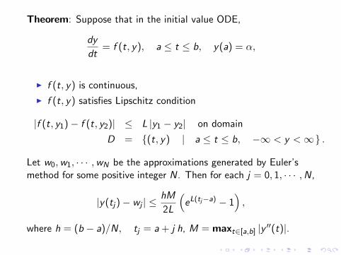
Theorem: Suppose that in the initial value ODE,
dy
dt= f (t, y), a ≤ t ≤ b, y(a) = α,
I f (t, y) is continuous,
I f (t, y) satisfies Lipschitz condition
|f (t, y1)− f (t, y2)| ≤ L |y1 − y2| on domain
D = {(t, y) | a ≤ t ≤ b, −∞ < y <∞} .
Let w0,w1, · · · ,wN be the approximations generated by Euler’smethod for some positive integer N. Then for each j = 0, 1, · · · ,N,
|y(tj)− wj | ≤hM
2L
(eL(tj−a) − 1
),
where h = (b − a)/N, tj = a + j h, M = maxt∈[a,b] |y ′′(t)|.
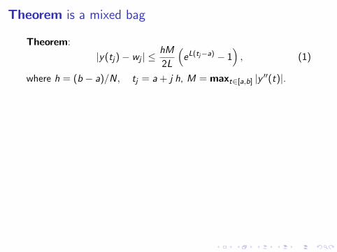
Theorem is a mixed bag
Theorem:
|y(tj)− wj | ≤hM
2L
(eL(tj−a) − 1
), (1)
where h = (b − a)/N, tj = a + j h, M = maxt∈[a,b] |y ′′(t)|.
How good is Theorem?
I Good News: Euler’s method converges:
limN→∞
hM
2L
(eL(tj−a) − 1
)= 0.
I Bad News: N may have to be impossibly large:
eL(tN−a) = eL(b−a) > 1043 if L > 10 and b − a > 10.

Theorem: Suppose that in the initial value ODE,
dy
dt= f (t, y), a ≤ t ≤ b, y(a) = α,
I f (t, y) is continuous,
I f (t, y) satisfies Lipschitz condition
|f (t, y1)− f (t, y2)| ≤ L |y1 − y2| on domain
D = {(t, y) | a ≤ t ≤ b, −∞ < y <∞} .
Let w0,w1, · · · ,wN be the approximations generated by Euler’smethod for some positive integer N. Then for each j = 0, 1, · · · ,N,
|y(tj)− wj | ≤hM
2L
(eL(tj−a) − 1
),
where h = (b − a)/N, tj = a + j h, M = maxt∈[a,b] |y ′′(t)|.

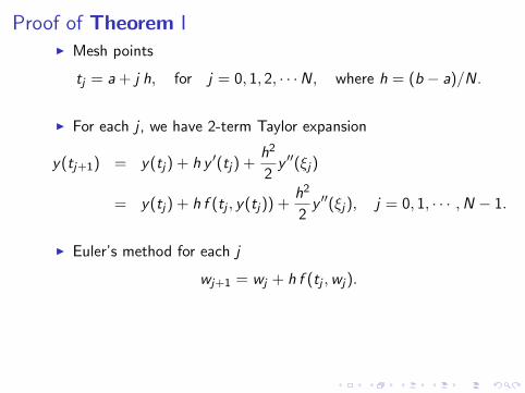
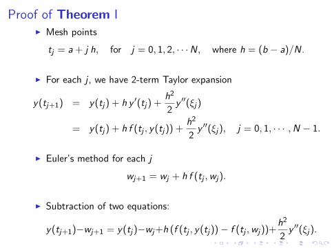
Proof of Theorem II Mesh points
tj = a + j h, for j = 0, 1, 2, · · ·N, where h = (b − a)/N.
I For each j , we have 2-term Taylor expansion
y(tj+1) = y(tj) + h y ′(tj) +h2
2y ′′(ξj)
= y(tj) + h f (tj , y(tj)) +h2
2y ′′(ξj), j = 0, 1, · · · ,N − 1.
I Euler’s method for each j
wj+1 = wj + h f (tj ,wj).
I Subtraction of two equations:
y(tj+1)−wj+1 = y(tj)−wj+h (f (tj , y(tj))− f (tj ,wj))+h2
2y ′′(ξj).

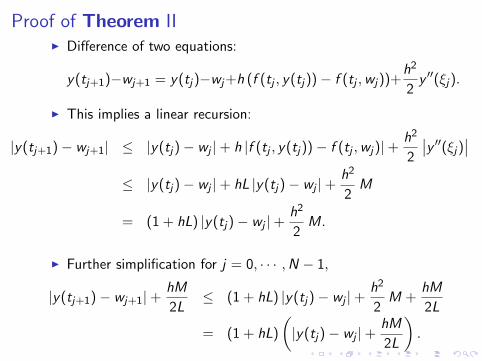
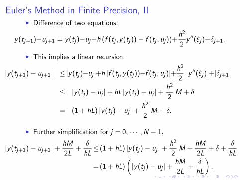
Proof of Theorem III Difference of two equations:
y(tj+1)−wj+1 = y(tj)−wj+h (f (tj , y(tj))− f (tj ,wj))+h2
2y ′′(ξj).
I This implies a linear recursion:
|y(tj+1)− wj+1| ≤ |y(tj)− wj |+ h |f (tj , y(tj))− f (tj ,wj)|+h2
2
∣∣y ′′(ξj)∣∣≤ |y(tj)− wj |+ hL |y(tj)− wj |+
h2
2M
= (1 + hL) |y(tj)− wj |+h2
2M.
I Further simplification for j = 0, · · · ,N − 1,
|y(tj+1)− wj+1|+hM
2L≤ (1 + hL) |y(tj)− wj |+
h2
2M +
hM
2L
= (1 + hL)
(|y(tj)− wj |+
hM
2L
).
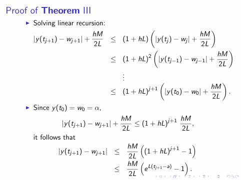
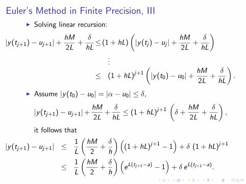
Proof of Theorem IIII Solving linear recursion:
|y(tj+1)− wj+1|+hM
2L≤ (1 + hL)
(|y(tj)− wj |+
hM
2L
)≤ (1 + hL)2
(|y(tj−1)− wj−1|+
hM
2L
)...
≤ (1 + hL)j+1
(|y(t0)− w0|+
hM
2L
).
I Since y(t0) = w0 = α,
|y(tj+1)− wj+1|+hM
2L≤ (1 + hL)j+1 hM
2L,
it follows that
|y(tj+1)− wj+1| ≤hM
2L
((1 + hL)j+1 − 1
)≤ hM
2L
(eL(tj+1−a) − 1
).
Theorem: Suppose that in the initial value ODE,
dy
dt= f (t, y), a ≤ t ≤ b, y(a) = α,
I f (t, y) is continuous,
I f (t, y) satisfies Lipschitz condition
|f (t, y1)− f (t, y2)| ≤ L |y1 − y2| on domain
D = {(t, y) | a ≤ t ≤ b, −∞ < y <∞} .
Let w0,w1, · · · ,wN be the approximations generated by Euler’smethod for some positive integer N. Then for each j = 0, 1, · · · ,N,
|y(tj)− wj | ≤hM
2L
(eL(tj−a) − 1
),
where h = (b − a)/N, tj = a + j h, M = maxt∈[a,b] |y ′′(t)|.

Euler’s Method: example (I)
Initial Value ODEdy
dt= y − t2 + 1, 0 ≤ t ≤ 2, y(0) = 0.5,
exact solution y(t) = (1 + t)2 − 0.5 et .
I Choose positive integer N = 10, so
h = 0.2, tj = 0.2 j , for j = 0, 1, 2, · · · 10.
I Set w0 = 0.5. For j = 0, 1, · · · , 9,
wj+1 = wj + h (wj − t2j + 1) = wj + 0.2(wi − 0.04j2 + 1)
= 1.2wj − 0.008j2 + 0.2.
Since y ′′(t) = 2− 0.5 et ,∂f
∂y(t, y) = 1,
it follows that∣∣y ′′(t)
∣∣ ≤ 0.5 e2 − 2def= M, L = 1.
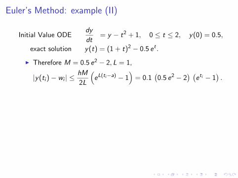
Euler’s Method: example (II)
Initial Value ODEdy
dt= y − t2 + 1, 0 ≤ t ≤ 2, y(0) = 0.5,
exact solution y(t) = (1 + t)2 − 0.5 et .
I Therefore M = 0.5 e2 − 2, L = 1,
|y(ti )− wi | ≤hM
2L
(eL(ti−a) − 1
)= 0.1
(0.5 e2 − 2
) (eti − 1
).

Euler’s Method: example (II)
Initial Value ODEdy
dt= y − t2 + 1, 0 ≤ t ≤ 2, y(0) = 0.5,
exact solution y(t) = (1 + t)2 − 0.5 et .
I Therefore M = 0.5 e2 − 2, L = 1,
|y(ti )− wi | ≤hM
2L
(eL(ti−a) − 1
)= 0.1
(0.5 e2 − 2
) (eti − 1
).
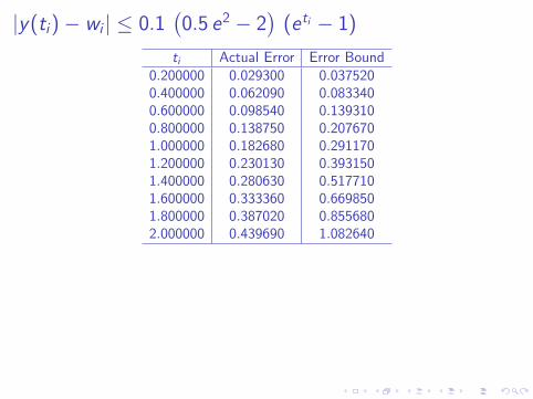
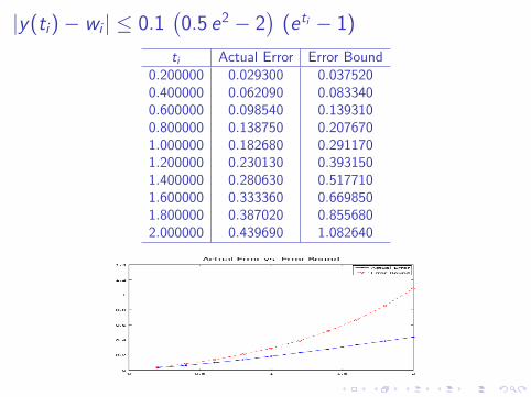
|y(ti)− wi | ≤ 0.1(0.5 e2 − 2
)(eti − 1)
ti Actual Error Error Bound0.200000 0.029300 0.0375200.400000 0.062090 0.0833400.600000 0.098540 0.1393100.800000 0.138750 0.2076701.000000 0.182680 0.2911701.200000 0.230130 0.3931501.400000 0.280630 0.5177101.600000 0.333360 0.6698501.800000 0.387020 0.8556802.000000 0.439690 1.082640
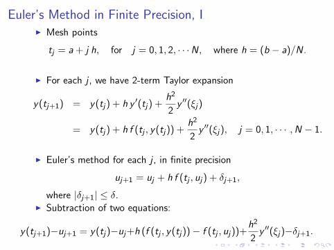
Euler’s Method in Finite Precision, II Mesh points
tj = a + j h, for j = 0, 1, 2, · · ·N, where h = (b − a)/N.
I For each j , we have 2-term Taylor expansion
y(tj+1) = y(tj) + h y ′(tj) +h2
2y ′′(ξj)
= y(tj) + h f (tj , y(tj)) +h2
2y ′′(ξj), j = 0, 1, · · · ,N − 1.
I Euler’s method for each j , in finite precision
uj+1 = uj + h f (tj , uj) + δj+1,
where |δj+1| ≤ δ.I Subtraction of two equations:
y(tj+1)−uj+1 = y(tj)−uj+h (f (tj , y(tj))− f (tj , uj))+h2
2y ′′(ξj)−δj+1.

Euler’s Method in Finite Precision, II Mesh points
tj = a + j h, for j = 0, 1, 2, · · ·N, where h = (b − a)/N.
I For each j , we have 2-term Taylor expansion
y(tj+1) = y(tj) + h y ′(tj) +h2
2y ′′(ξj)
= y(tj) + h f (tj , y(tj)) +h2
2y ′′(ξj), j = 0, 1, · · · ,N − 1.
I Euler’s method for each j , in finite precision
uj+1 = uj + h f (tj , uj) + δj+1,
where |δj+1| ≤ δ.
I Subtraction of two equations:
y(tj+1)−uj+1 = y(tj)−uj+h (f (tj , y(tj))− f (tj , uj))+h2
2y ′′(ξj)−δj+1.
Euler’s Method in Finite Precision, II Mesh points
tj = a + j h, for j = 0, 1, 2, · · ·N, where h = (b − a)/N.
I For each j , we have 2-term Taylor expansion
y(tj+1) = y(tj) + h y ′(tj) +h2
2y ′′(ξj)
= y(tj) + h f (tj , y(tj)) +h2
2y ′′(ξj), j = 0, 1, · · · ,N − 1.
I Euler’s method for each j , in finite precision
uj+1 = uj + h f (tj , uj) + δj+1,
where |δj+1| ≤ δ.I Subtraction of two equations:
y(tj+1)−uj+1 = y(tj)−uj+h (f (tj , y(tj))− f (tj , uj))+h2
2y ′′(ξj)−δj+1.

Euler’s Method in Finite Precision, III Difference of two equations:
y(tj+1)−uj+1 = y(tj)−uj+h (f (tj , y(tj))− f (tj , uj))+h2
2y ′′(ξj)−δj+1.
I This implies a linear recursion:
|y(tj+1)− uj+1| ≤ |y(tj)−uj |+h |f (tj , y(tj))−f (tj , uj)|+h2
2
∣∣y ′′(ξj)∣∣+|δj+1|
≤ |y(tj)− uj |+ hL |y(tj)− uj |+h2
2M + δ
= (1 + hL) |y(tj)− uj |+h2
2M + δ.
I Further simplification for j = 0, · · · ,N − 1,
|y(tj+1)− uj+1|+hM
2L+
δ
hL≤ (1 + hL) |y(tj)− uj |+
h2
2M +
hM
2L+ δ +
δ
hL
= (1 + hL)
(|y(tj)− uj |+
hM
2L+
δ
hL
).
Euler’s Method in Finite Precision, IIII Solving linear recursion:
|y(tj+1)− uj+1|+hM
2L+
δ
hL≤ (1 + hL)
(|y(tj)− uj |+
hM
2L+
δ
hL
)...
≤ (1 + hL)j+1
(|y(t0)− u0|+
hM
2L+
δ
hL
).
I Assume |y(t0)− u0| = |α− u0| ≤ δ,
|y(tj+1)− uj+1|+hM
2L+
δ
hL≤ (1 + hL)j+1
(δ +
hM
2L+
δ
hL
),
it follows that
|y(tj+1)− uj+1| ≤1
L
(hM
2+δ
h
)((1 + hL)j+1 − 1
)+ δ (1 + hL)j+1
≤ 1
L
(hM
2+δ
h
)(eL(tj+1−a) − 1
)+ δ eL(tj+1−a).

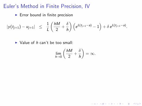
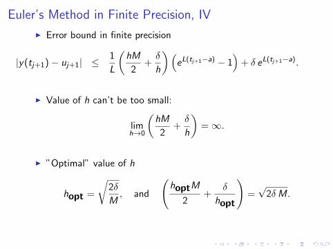
Euler’s Method in Finite Precision, IV
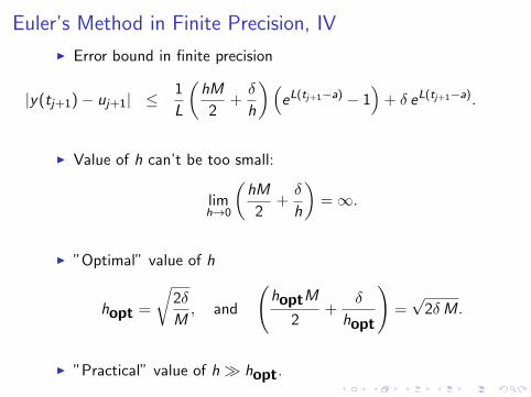
I Error bound in finite precision
|y(tj+1)− uj+1| ≤1
L
(hM
2+δ
h
)(eL(tj+1−a) − 1
)+ δ eL(tj+1−a).
I Value of h can’t be too small:
limh→0
(hM
2+δ
h
)=∞.
I ”Optimal” value of h
hopt =
√2δ
M, and
(hoptM
2+
δ
hopt
)=√
2δM.
I ”Practical” value of h� hopt.
Euler’s Method in Finite Precision, IV
I Error bound in finite precision
|y(tj+1)− uj+1| ≤1
L
(hM
2+δ
h
)(eL(tj+1−a) − 1
)+ δ eL(tj+1−a).
I Value of h can’t be too small:
limh→0
(hM
2+δ
h
)=∞.
I ”Optimal” value of h
hopt =
√2δ
M, and
(hoptM
2+
δ
hopt
)=√
2δM.
I ”Practical” value of h� hopt.
Euler’s Method in Finite Precision, IV
I Error bound in finite precision
|y(tj+1)− uj+1| ≤1
L
(hM
2+δ
h
)(eL(tj+1−a) − 1
)+ δ eL(tj+1−a).
I Value of h can’t be too small:
limh→0
(hM
2+δ
h
)=∞.
I ”Optimal” value of h
hopt =
√2δ
M, and
(hoptM
2+
δ
hopt
)=√
2δM.
I ”Practical” value of h� hopt.
Euler’s Method in Finite Precision, IV
I Error bound in finite precision
|y(tj+1)− uj+1| ≤1
L
(hM
2+δ
h
)(eL(tj+1−a) − 1
)+ δ eL(tj+1−a).
I Value of h can’t be too small:
limh→0
(hM
2+δ
h
)=∞.
I ”Optimal” value of h
hopt =
√2δ
M, and
(hoptM
2+
δ
hopt
)=√
2δM.
I ”Practical” value of h� hopt.
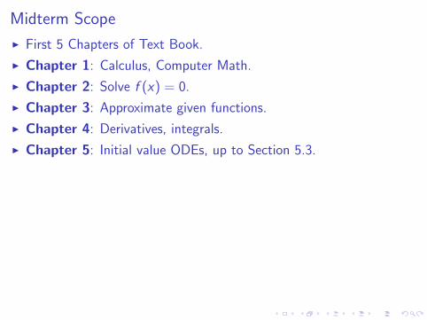
Midterm Scope
I First 5 Chapters of Text Book.
I Chapter 1: Calculus, Computer Math.
I Chapter 2: Solve f (x) = 0.
I Chapter 3: Approximate given functions.
I Chapter 4: Derivatives, integrals.
I Chapter 5: Initial value ODEs, up to Section 5.3.

Review: Midterm rules
I No calculators.
I one-sided one-page cheat sheet.
I exam problems are mostly (modified) from exercises intextbook.
I free to use results in the proper text, but not anything else.

Chapter 1
I CalculusI Extreme Value TheoremI Mean Value TheoremI Intermediate Value Theorem
I Machine PrecisionI Round-off errorsI Stable quadratic rootsI Numerical stability
I Rate of convergence: the Big O
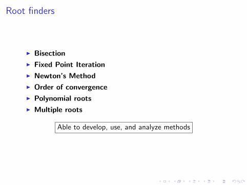
Root finders
I Bisection
I Fixed Point Iteration
I Newton’s Method
I Order of convergence
I Polynomial roots
I Multiple roots
Able to develop, use, and analyze methods

Interpolation and Polynomial Approximation
I Interpolation and the Lagrange Polynomial
I Error Analysis
I Divided Differences
I Hermite Interpolation
I Cubic Spline Interpolation
Able to develop and analyze approximation methods

Numerical Differentiation and Integration
I Numerical Differentiation
I Extrapolation
I Trapezoidal/Simpson rules, DoP
I Composite Numerical Integration
I Adaptive Quadrature, error bounds vs. estimates
I Gaussian Quadrature
I Multiple/Improper Integrals
Able to develop and analyze basic integration methods

Initial-Value Problems for ODEs
I Elementary Theory of Initial-Value Problems, Lipschitzconditions
I Euler’s Method
I Higher-Order Taylor Methods
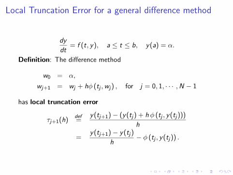
Local Truncation Error for a general difference method
dy
dt= f (t, y), a ≤ t ≤ b, y(a) = α.
Definition: The difference method
w0 = α,
wj+1 = wj + hφ (tj ,wj) , for j = 0, 1, · · · ,N − 1
has local truncation error
τj+1(h)def=
y(tj+1)− (y(tj) + h φ (tj , y(tj)))
h
=y(tj+1)− y(tj)
h− φ (tj , y(tj)) .
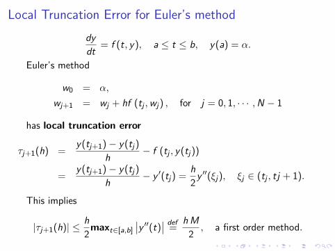
Local Truncation Error for Euler’s method
dy
dt= f (t, y), a ≤ t ≤ b, y(a) = α.
Euler’s method
w0 = α,
wj+1 = wj + hf (tj ,wj) , for j = 0, 1, · · · ,N − 1
has local truncation error
τj+1(h) =y(tj+1)− y(tj)
h− f (tj , y(tj))
=y(tj+1)− y(tj)
h− y ′(tj) =
h
2y ′′(ξj), ξj ∈ (tj , tj + 1).
This implies
|τj+1(h)| ≤ h
2maxt∈[a,b]
∣∣y ′′(t)∣∣ def=
hM
2, a first order method.

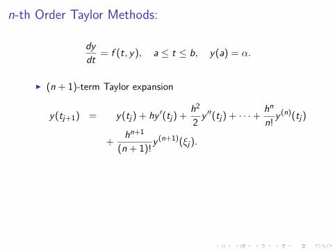
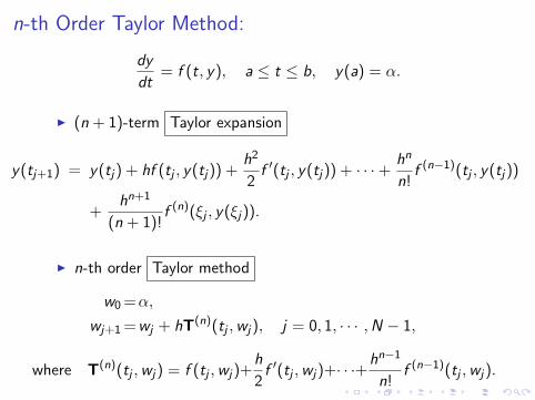
n-th Order Taylor Methods:
dy
dt= f (t, y), a ≤ t ≤ b, y(a) = α.
I (n + 1)-term Taylor expansion
y(tj+1) = y(tj) + hy ′(tj) +h2
2y ′′(tj) + · · ·+ hn
n!y (n)(tj)
+hn+1
(n + 1)!y (n+1)(ξj).
I On the other hand,
y ′(tj) = f (tj , y(tj)), y ′′(tj) = f ′(tj , y(tj)), · · ·y (n)(tj) = f (n−1)(tj , y(tj)).
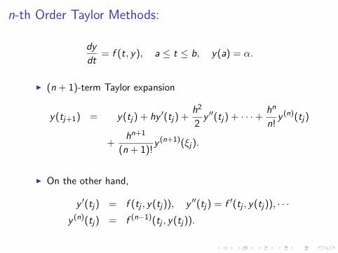

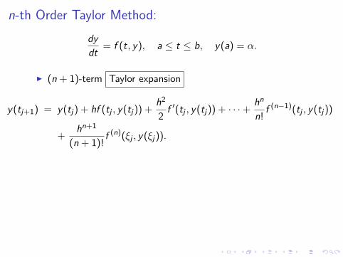
n-th Order Taylor Method:
dy
dt= f (t, y), a ≤ t ≤ b, y(a) = α.
I (n + 1)-term Taylor expansion
y(tj+1) = y(tj) + hf (tj , y(tj)) +h2
2f ′(tj , y(tj)) + · · ·+ hn
n!f (n−1)(tj , y(tj))
+hn+1
(n + 1)!f (n)(ξj , y(ξj)).
I n-th order Taylor method
w0 =α,
wj+1 =wj + hT(n)(tj ,wj), j = 0, 1, · · · ,N − 1,
where T(n)(tj ,wj) = f (tj ,wj)+h
2f ′(tj ,wj)+· · ·+hn−1
n!f (n−1)(tj ,wj).
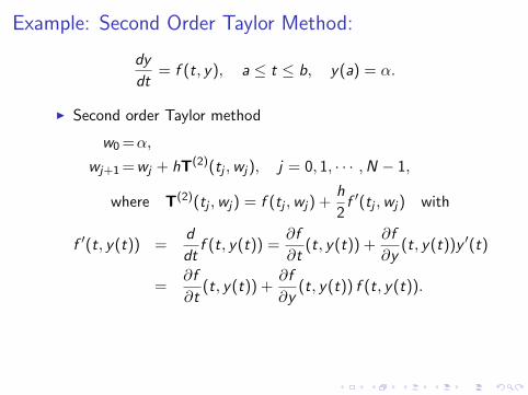
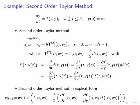
Example: Second Order Taylor Method:
dy
dt= f (t, y), a ≤ t ≤ b, y(a) = α.
I Second order Taylor method
w0 =α,
wj+1 =wj + hT(2)(tj ,wj), j = 0, 1, · · · ,N − 1,
where T(2)(tj ,wj) = f (tj ,wj) +h
2f ′(tj ,wj) with
f ′(t, y(t)) =d
dtf (t, y(t)) =
∂f
∂t(t, y(t)) +
∂f
∂y(t, y(t))y ′(t)
=∂f
∂t(t, y(t)) +
∂f
∂y(t, y(t)) f (t, y(t)).
I Second order Taylor method in explicit form
wj+1 =wj + h
(f (tj ,wj) +
h
2
(∂f
∂t(tj ,wj) +
∂f
∂y(tj ,wj) f ((tj ,wj))
)).
Example: Second Order Taylor Method:
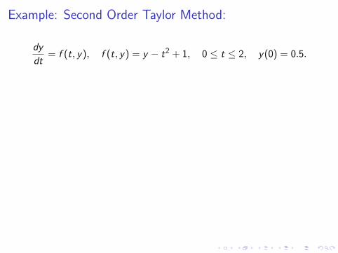
dy
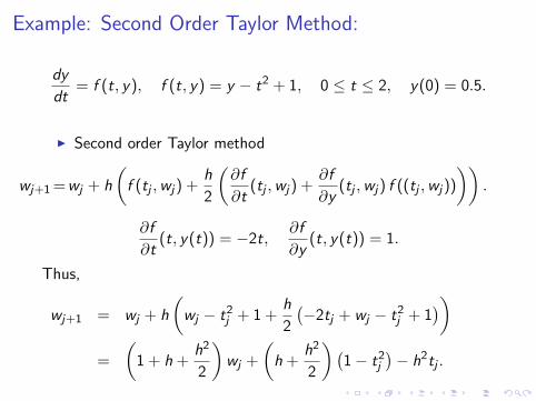
dt= f (t, y), f (t, y) = y − t2 + 1, 0 ≤ t ≤ 2, y(0) = 0.5.
I Second order Taylor method
wj+1 =wj + h
(f (tj ,wj) +
h
2
(∂f
∂t(tj ,wj) +
∂f
∂y(tj ,wj) f ((tj ,wj))
)).
∂f
∂t(t, y(t)) = −2t,
∂f
∂y(t, y(t)) = 1.
Thus,
wj+1 = wj + h
(wj − t2j + 1 +
h
2
(−2tj + wj − t2j + 1
))=
(1 + h +
h2
2
)wj +
(h +
h2
2
)(1− t2j
)− h2tj .
Example: Second Order Taylor Method:
dy
dt= f (t, y), f (t, y) = y − t2 + 1, 0 ≤ t ≤ 2, y(0) = 0.5.
I Second order Taylor method
wj+1 =wj + h
(f (tj ,wj) +
h
2
(∂f
∂t(tj ,wj) +
∂f
∂y(tj ,wj) f ((tj ,wj))
)).
∂f
∂t(t, y(t)) = −2t,
∂f
∂y(t, y(t)) = 1.
Thus,
wj+1 = wj + h
(wj − t2j + 1 +
h
2
(−2tj + wj − t2j + 1
))=
(1 + h +
h2
2
)wj +
(h +
h2
2
)(1− t2j
)− h2tj .

Euler’s Method vs. Second Order Taylor Method: N = 10
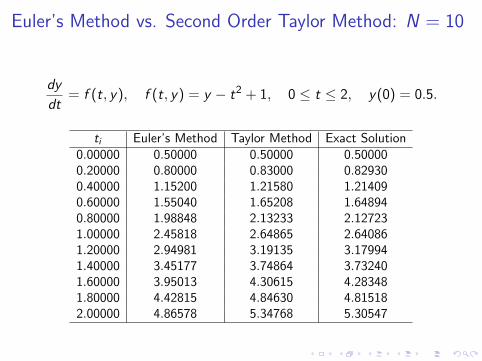
dy
dt= f (t, y), f (t, y) = y − t2 + 1, 0 ≤ t ≤ 2, y(0) = 0.5.
ti Euler’s Method Taylor Method Exact Solution0.00000 0.50000 0.50000 0.500000.20000 0.80000 0.83000 0.829300.40000 1.15200 1.21580 1.214090.60000 1.55040 1.65208 1.648940.80000 1.98848 2.13233 2.127231.00000 2.45818 2.64865 2.640861.20000 2.94981 3.19135 3.179941.40000 3.45177 3.74864 3.732401.60000 3.95013 4.30615 4.283481.80000 4.42815 4.84630 4.815182.00000 4.86578 5.34768 5.30547
Euler’s Method vs. Second Order Taylor Method: N = 10
dy
dt= f (t, y), f (t, y) = y − t2 + 1, 0 ≤ t ≤ 2, y(0) = 0.5.
ti Euler’s Method Taylor Method Exact Solution0.00000 0.50000 0.50000 0.500000.20000 0.80000 0.83000 0.829300.40000 1.15200 1.21580 1.214090.60000 1.55040 1.65208 1.648940.80000 1.98848 2.13233 2.127231.00000 2.45818 2.64865 2.640861.20000 2.94981 3.19135 3.179941.40000 3.45177 3.74864 3.732401.60000 3.95013 4.30615 4.283481.80000 4.42815 4.84630 4.815182.00000 4.86578 5.34768 5.30547

Euler’s Method vs. Second Order Taylor Method: N = 10I Second order method looks more accurate.
I Second order method has much smaller errors.

Euler’s Method vs. Second Order Taylor Method: N = 10I Second order method looks more accurate.
I Second order method has much smaller errors.

Runge-Kutta methods
With orders of Taylor methods yet without derivatives of f (t, y(t))
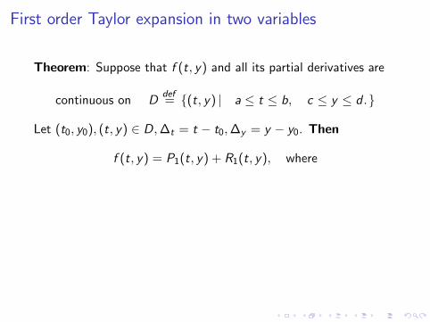
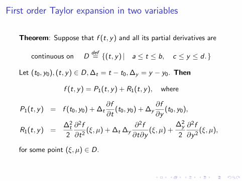
First order Taylor expansion in two variables
Theorem: Suppose that f (t, y) and all its partial derivatives are
continuous on Ddef= {(t, y) | a ≤ t ≤ b, c ≤ y ≤ d .}
Let (t0, y0), (t, y) ∈ D,∆t = t − t0,∆y = y − y0. Then
f (t, y) = P1(t, y) + R1(t, y), where
P1(t, y) = f (t0, y0) + ∆t∂f
∂t(t0, y0) + ∆y
∂f
∂y(t0, y0),
R1(t, y) =∆2
t
2
∂2f
∂t2(ξ, µ) + ∆t ∆y
∂2f
∂t∂y(ξ, µ) +
∆2y
2
∂2f
∂y2(ξ, µ),
for some point (ξ, µ) ∈ D.
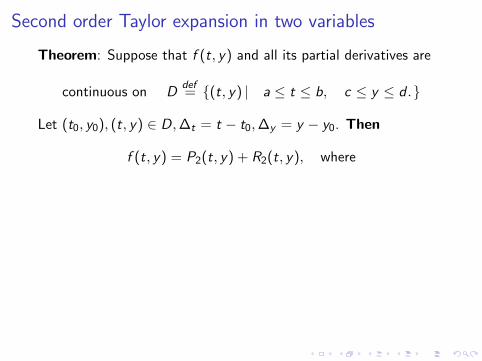
Second order Taylor expansion in two variables
Theorem: Suppose that f (t, y) and all its partial derivatives are
continuous on Ddef= {(t, y) | a ≤ t ≤ b, c ≤ y ≤ d .}
Let (t0, y0), (t, y) ∈ D,∆t = t − t0,∆y = y − y0. Then
f (t, y) = P2(t, y) + R2(t, y), where
P2(t, y) = f (t0, y0) +
(∆t
∂f
∂t(t0, y0) + ∆y
∂f
∂y(t0, y0)
)+
(∆2
t
2
∂2f
∂t2(t0, y0) + ∆t ∆y
∂2f
∂t∂y(t0, y0) +
∆2y
2
∂2f
∂y2(t0, y0)
),
R2(t, y) =1
3!
3∑j=0
(3j
)∆3−j
t ∆jy
∂3f
∂t3−j∂y j(ξ, µ)
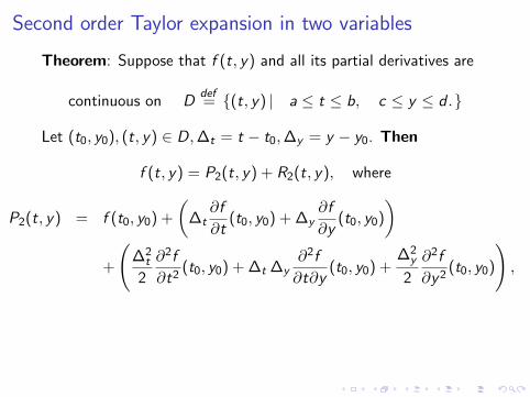

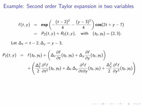
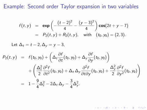
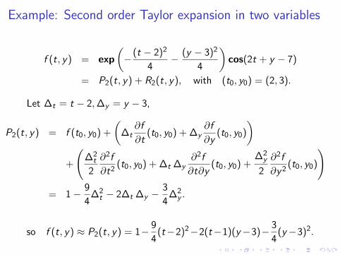
Example: Second order Taylor expansion in two variables
f (t, y) = exp
(−(t − 2)2
4− (y − 3)2
4
)cos(2t + y − 7)
= P2(t, y) + R2(t, y), with (t0, y0) = (2, 3).
Let ∆t = t − 2,∆y = y − 3,
P2(t, y) = f (t0, y0) +
(∆t
∂f
∂t(t0, y0) + ∆y
∂f
∂y(t0, y0)
)+
(∆2
t
2
∂2f
∂t2(t0, y0) + ∆t ∆y
∂2f
∂t∂y(t0, y0) +
∆2y
2
∂2f
∂y2(t0, y0)
)= 1− 9
4∆2
t − 2∆t ∆y −3
4∆2
y .
so f (t, y) ≈ P2(t, y) = 1− 9
4(t−2)2−2(t−1)(y−3)− 3
4(y−3)2.
Example: Second order Taylor expansion in two variables
f (t, y) = exp
(−(t − 2)2
4− (y − 3)2
4
)cos(2t + y − 7)
= P2(t, y) + R2(t, y), with (t0, y0) = (2, 3).
Let ∆t = t − 2,∆y = y − 3,
P2(t, y) = f (t0, y0) +
(∆t
∂f
∂t(t0, y0) + ∆y
∂f
∂y(t0, y0)
)+
(∆2
t
2
∂2f
∂t2(t0, y0) + ∆t ∆y
∂2f
∂t∂y(t0, y0) +
∆2y
2
∂2f
∂y2(t0, y0)
)
= 1− 9
4∆2
t − 2∆t ∆y −3
4∆2
y .
so f (t, y) ≈ P2(t, y) = 1− 9
4(t−2)2−2(t−1)(y−3)− 3
4(y−3)2.
Example: Second order Taylor expansion in two variables
f (t, y) = exp
(−(t − 2)2
4− (y − 3)2
4
)cos(2t + y − 7)
= P2(t, y) + R2(t, y), with (t0, y0) = (2, 3).
Let ∆t = t − 2,∆y = y − 3,
P2(t, y) = f (t0, y0) +
(∆t
∂f
∂t(t0, y0) + ∆y
∂f
∂y(t0, y0)
)+
(∆2
t
2
∂2f
∂t2(t0, y0) + ∆t ∆y
∂2f
∂t∂y(t0, y0) +
∆2y
2
∂2f
∂y2(t0, y0)
)= 1− 9
4∆2
t − 2∆t ∆y −3
4∆2
y .
so f (t, y) ≈ P2(t, y) = 1− 9
4(t−2)2−2(t−1)(y−3)− 3
4(y−3)2.
Example: Second order Taylor expansion in two variables
f (t, y) = exp
(−(t − 2)2
4− (y − 3)2
4
)cos(2t + y − 7)
= P2(t, y) + R2(t, y), with (t0, y0) = (2, 3).
Let ∆t = t − 2,∆y = y − 3,
P2(t, y) = f (t0, y0) +
(∆t
∂f
∂t(t0, y0) + ∆y
∂f
∂y(t0, y0)
)+
(∆2
t
2
∂2f
∂t2(t0, y0) + ∆t ∆y
∂2f
∂t∂y(t0, y0) +
∆2y
2
∂2f
∂y2(t0, y0)
)= 1− 9
4∆2
t − 2∆t ∆y −3
4∆2
y .
so f (t, y) ≈ P2(t, y) = 1− 9
4(t−2)2−2(t−1)(y−3)− 3
4(y−3)2.

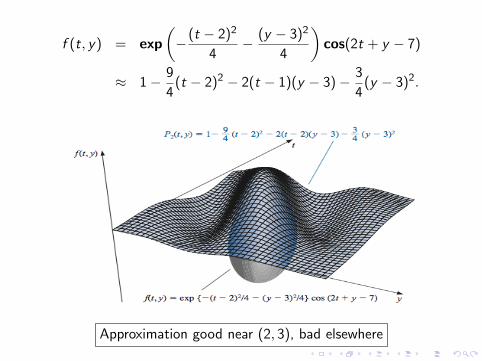
f (t, y) = exp
(−(t − 2)2
4− (y − 3)2
4
)cos(2t + y − 7)
≈ 1− 9
4(t − 2)2 − 2(t − 1)(y − 3)− 3
4(y − 3)2.
Approximation good near (2, 3), bad elsewhere
f (t, y) = exp
(−(t − 2)2
4− (y − 3)2
4
)cos(2t + y − 7)
≈ 1− 9
4(t − 2)2 − 2(t − 1)(y − 3)− 3
4(y − 3)2.
Approximation good near (2, 3), bad elsewhere
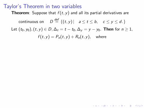
Taylor’s Theorem in two variablesTheorem: Suppose that f (t, y) and all its partial derivatives are
continuous on Ddef= {(t, y) | a ≤ t ≤ b, c ≤ y ≤ d .}
Let (t0, y0), (t, y) ∈ D,∆t = t − t0,∆y = y − y0. Then for n ≥ 1,
f (t, y) = Pn(t, y) + Rn(t, y), where
Pn(t, y) = f (t0, y0) +
(∆t
∂f
∂t(t0, y0) + ∆y
∂f
∂y(t0, y0)
)+
(∆2
t
2
∂2f
∂t2(t0, y0) + ∆t ∆y
∂2f
∂t∂y(t0, y0) +
∆2y
2
∂2f
∂y2(t0, y0)
)
+ · · ·+ 1
n!
n∑j=0
(nj
)∆n−j
t ∆jy
∂nf
∂tn−j∂y j(t0, y0)
,
Rn(t, y) =1
(n + 1)!
n+1∑j=0
(n + 1j
)∆n+1−j
t ∆jy
∂n+1f
∂tn+1−j∂y j(ξ, µ)
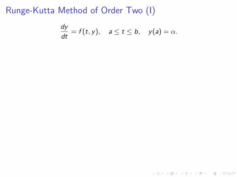
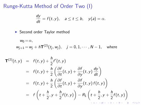
Runge-Kutta Method of Order Two (I)
dy
dt= f (t, y), a ≤ t ≤ b, y(a) = α.
I Second order Taylor method
w0 =α,
wj+1 =wj + hT(2)(tj ,wj), j = 0, 1, · · · ,N − 1, where
T(2)(t, y) = f (t, y) +h
2f ′(t, y)
= f (t, y) +h
2
(∂f
∂t(t, y) +
∂f
∂y(t, y)
dy
dt
)= f (t, y) +
h
2
(∂f
∂t(t, y) +
∂f
∂y(t, y) f (t, y)
)= f
(t +
h
2, y +
h
2f (t, y)
)− R1
(t +
h
2, y +
h
2f (t, y)
)

Runge-Kutta Method of Order Two (II)
I Second order Taylor method
w0 =α,
wj+1 =wj + hT(2)(tj ,wj), j = 0, 1, · · · ,N − 1, where
T(2)(t, y) = f
(t +
h
2, y +
h
2f (t, y)
)− R1
(t +
h
2, y +
h
2f (t, y)
),
I From first order Taylor expansion,
R1
(t +
h
2, y +
h
2f (t, y)
)=
h2
8
∂2f
∂t2(ξ, µ) +
h2f (t, y)
4∆t ∆y
∂2f
∂t∂y(ξ, µ)
+h2f 2(t, y)
8
∂2f
∂y2(ξ, µ) = O(h2).
Method remains second order after dropping R1
(t + h
2 , y + h2 f (t, y)
)
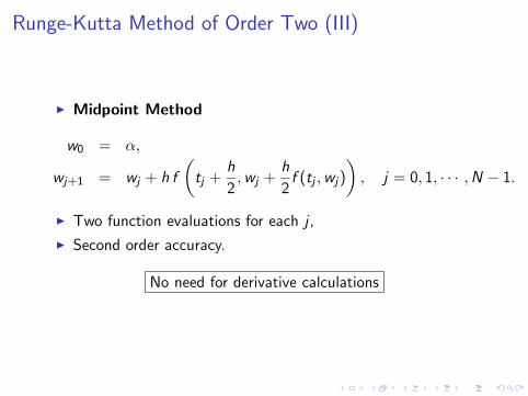
Runge-Kutta Method of Order Two (III)
I Midpoint Method
w0 = α,
wj+1 = wj + h f
(tj +
h
2,wj +
h
2f (tj ,wj)
), j = 0, 1, · · · ,N − 1.
I Two function evaluations for each j ,
I Second order accuracy.
No need for derivative calculations
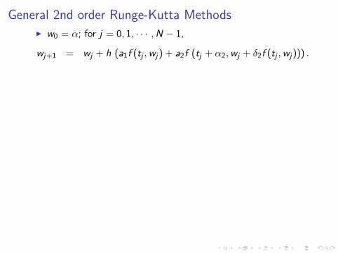
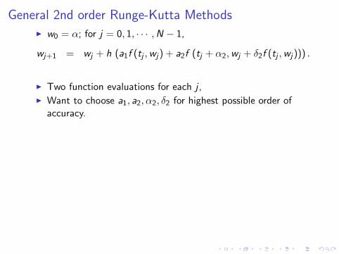
General 2nd order Runge-Kutta MethodsI w0 = α; for j = 0, 1, · · · ,N − 1,
wj+1 = wj + h (a1f (tj ,wj) + a2f (tj + α2,wj + δ2f (tj ,wj))) .
I Two function evaluations for each j ,I Want to choose a1, a2, α2, δ2 for highest possible order of
accuracy.
local truncation error
τj+1(h) =y(tj+1)−y(tj)
h− (a1f (tj , y(tj))+a2f (tj+α2, y(tj)+δ2f (tj , y(tj))))
= y ′(tj) +h
2y ′′(tj) + O(h2)
−(
(a1 + a2) f (tj , y(tj)) + a2 α2∂f
∂t(tj , y(tj))
+ a2 δ2f (tj , y(tj))∂f
∂y(tj , y(tj)) + O(h2)
).
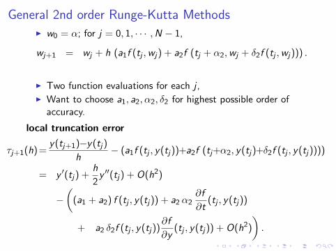
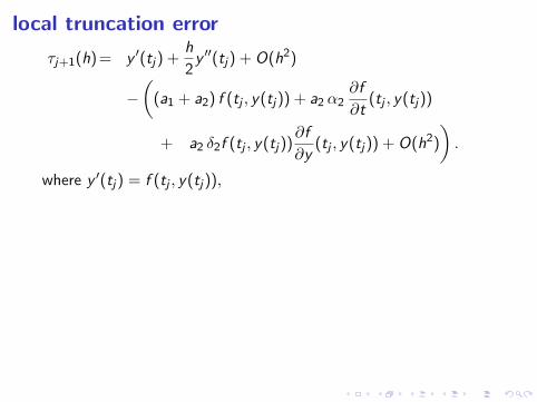
local truncation error
τj+1(h) = y ′(tj) +h
2y ′′(tj) + O(h2)
−(
(a1 + a2) f (tj , y(tj)) + a2 α2∂f
∂t(tj , y(tj))
+ a2 δ2f (tj , y(tj))∂f
∂y(tj , y(tj)) + O(h2)
).
where y ′(tj) = f (tj , y(tj)),
y ′′(tj) =d f
d t(tj , y(tj)) =
∂f
∂t(tj , y(tj)) + f (tj , y(tj))
∂f
∂y(tj , y(tj)).
For any choice with
a1 + a2 = 1, a2 α2 = a2 δ2 =h
2,
we have a second order method
τj+1(h) = O(h2).
Four parameters, three equations

General 2nd order Runge-Kutta Methods
w0 = α; for j = 0, 1, · · · ,N − 1,
wj+1 = wj + h (a1f (tj ,wj) + a2f (tj + α2,wj + δ2f (tj ,wj))) .
a1 + a2 = 1, a2 α2 = a2 δ2 =h
2,
I Midpoint method: a1 = 0, a2 = 1, α2 = δ2 = h2 ,
wj+1 = wj + h f
(tj +
h
2,wj +
h
2f (tj ,wj)
).
I Modified Euler method: a1 = a2 = 12 , α2 = δ2 = h,
wj+1 = wj +h
2(f (tj ,wj) + f (tj+1,wj + hf (tj ,wj))) .
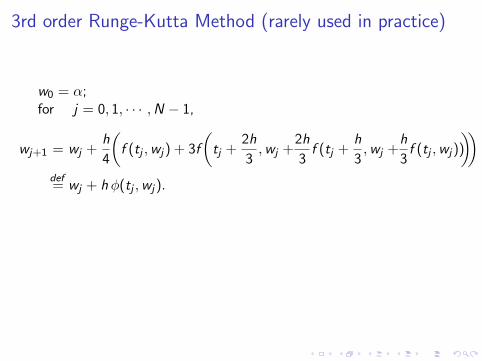
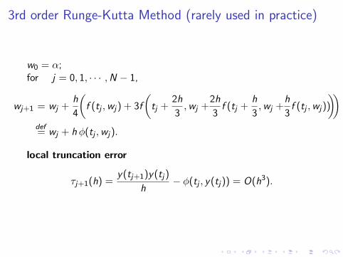
3rd order Runge-Kutta Method (rarely used in practice)
w0 = α;for j = 0, 1, · · · ,N − 1,
wj+1 = wj +h
4
(f (tj ,wj) + 3f
(tj +
2h
3,wj +
2h
3f (tj +
h
3,wj +
h
3f (tj ,wj))
))def= wj + h φ(tj ,wj).
local truncation error
τj+1(h) =y(tj+1)y(tj)
h− φ(tj , y(tj)) = O(h3).
3rd order Runge-Kutta Method (rarely used in practice)
w0 = α;for j = 0, 1, · · · ,N − 1,
wj+1 = wj +h
4
(f (tj ,wj) + 3f
(tj +
2h
3,wj +
2h
3f (tj +
h
3,wj +
h
3f (tj ,wj))
))def= wj + h φ(tj ,wj).
local truncation error
τj+1(h) =y(tj+1)y(tj)
h− φ(tj , y(tj)) = O(h3).

4th order Runge-Kutta Method
w0 = α;for j = 0, 1, · · · ,N − 1,
k1 = h f (tj ,wj),
k2 = h f
(tj +
h
2,wj +
1
2k1
),
k3 = h f
(tj +
h
2,wj +
1
2k2
),
k4 = h f (tj+1,wj + k3) ,
wj+1 = wj +1
6(k1 + 2k2 + 2k3 + k4) .
4 function evaluations per step
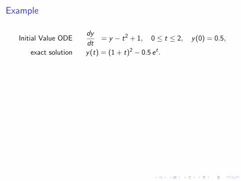
Example
Initial Value ODEdy
dt= y − t2 + 1, 0 ≤ t ≤ 2, y(0) = 0.5,
exact solution y(t) = (1 + t)2 − 0.5 et .

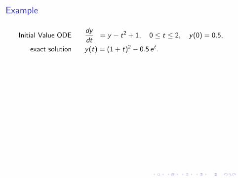
Example
Initial Value ODEdy
dt= y − t2 + 1, 0 ≤ t ≤ 2, y(0) = 0.5,
exact solution y(t) = (1 + t)2 − 0.5 et .
Example
Initial Value ODEdy
dt= y − t2 + 1, 0 ≤ t ≤ 2, y(0) = 0.5,
exact solution y(t) = (1 + t)2 − 0.5 et .

Example
Initial Value ODEdy
dt= y − t2 + 1, 0 ≤ t ≤ 2, y(0) = 0.5,
exact solution y(t) = (1 + t)2 − 0.5 et .


