

Lecture on atmospheric remote sensing [email protected]
Long Path (active) DOAS
-basic principle
-Long path DOAS (UV/vis/IR)
-instrumental improvements
-Specific applications
-white cell
-vertical profiles
-tomographic inversions

Lecture on atmospheric remote sensing [email protected]
A) Lambert-Beersches Gesetz: ( )I I c l= ⋅ − ⋅ ⋅0 exp σ
DOAS: ’Differentielle Optische AbsorptionsSpektroscopie’

Lecture on atmospheric remote sensing [email protected]
A) Lambert-Beersches Gesetz: ( )I I c l= ⋅ − ⋅ ⋅0 exp σ
DOAS: ’Differentielle Optische AbsorptionsSpektroscopie’
0
0.2
0.4
0.6
0.8
1
0 2 4 6 8 10Schichtdicke [km]
Rel
ativ
e In
tens
ität
Lichtabschwächung durch Ozon für UV-Licht bei 300nm
σ⋅
⎟⎠⎞⎜
⎝⎛
=l
II
c 0ln
Aus der Intensitätsmessung kann die Konzentration bestimmt werden

Lecture on atmospheric remote sensing [email protected]
SpiegelLichtquelle& Spektrograph
0.5 - 15 km
In der Realität ist es sehr ähnlich....
DOAS: ’Differentielle Optische AbsorptionsSpektroscopie’
A) Lambert-Beersches Gesetz: ( )I I c l= ⋅ − ⋅ ⋅0 exp σ

Lecture on atmospheric remote sensing [email protected]
Long Path DOAS
-basic principle
-Long path DOAS (UV/vis/IR)
-instrumental improvements
-Specific applications
-white cell
-vertical profiles
-tomographic inversions

Lecture on atmospheric remote sensing [email protected]
DOAS: ’Differentielle Optische AbsorptionsSpektroscopie’
SpiegelLichtquelle& Spektrograph
0.5 - 15 km

Lecture on atmospheric remote sensing [email protected]
http://http://wwwwww.chem..chem.leedsleeds..acac..ukuk/JMCP//JMCP/imagesimages//doaspicturedoaspicture..jpgjpg

Lecture on atmospheric remote sensing [email protected]
Typisches (früheres) LP-DOAS-Instrument
Spiegel Lichtquelle
Lecture on atmospheric remote sensing [email protected]
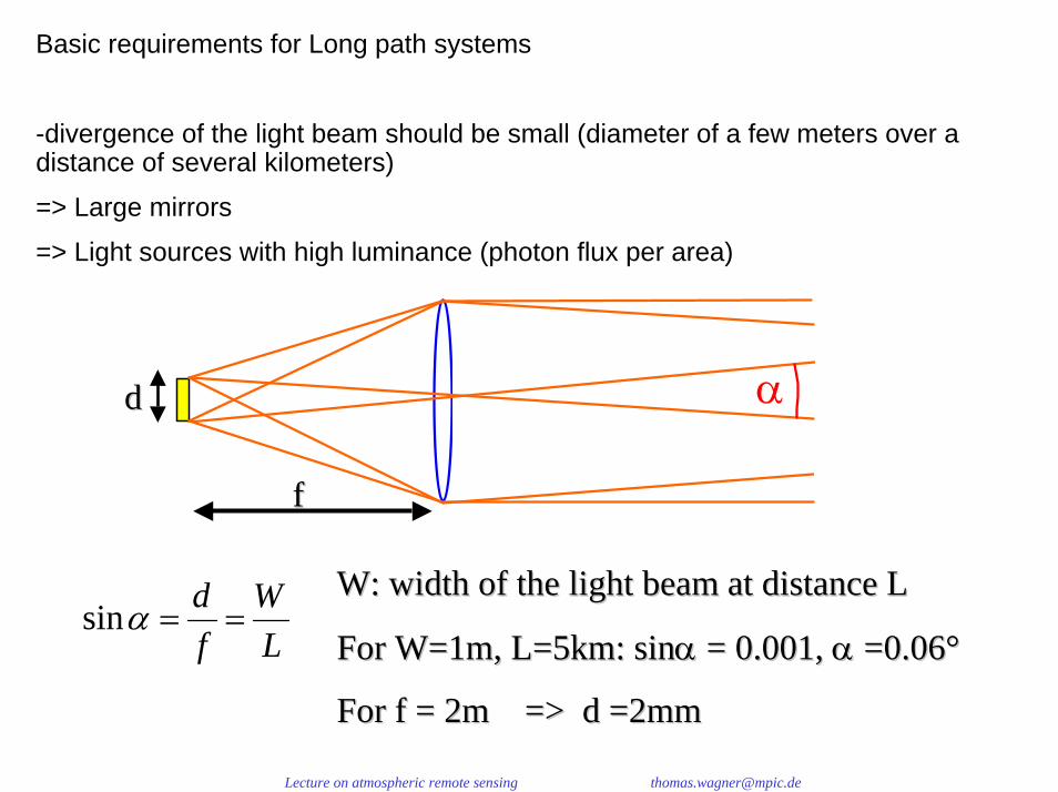
Basic requirements for Long path systems
-divergence of the light beam should be small (diameter of a few meters over a distance of several kilometers)
=> Large mirrors
=> Light sources with high luminance (photon flux per area)
αdd
ff
W:W: widthwidth ofof the light beamthe light beam at distance Lat distance L
For W=1m, L=5km:For W=1m, L=5km: sinsinαα = 0.001, = 0.001, αα =0.06°=0.06°
For f = 2m => d =2mm
LW
fd==αsin
For f = 2m => d =2mm

Lecture on atmospheric remote sensing [email protected]
Diplomarbeit Thorsten Hermes, IUP Heidelberg, 1999Diplomarbeit Thorsten Hermes, IUP Heidelberg, 1999

Der Druck der Xenon-Edelgasfüllung steigt während des Betriebs von etwa 8 bar im kalten Zustand auf bis zu 70 bar an.
Lecture on atmospheric remote sensing [email protected]

Lecture on atmospheric remote sensing [email protected]
Diplomarbeit Thorsten Hermes, IUP Heidelberg, 1999Diplomarbeit Thorsten Hermes, IUP Heidelberg, 1999

Lecture on atmospheric remote sensing [email protected]

Lecture on atmospheric remote sensing [email protected]
Diplomarbeit Jens Tschritter, IUP Heidelberg, 2007

Lecture on atmospheric remote sensing [email protected]

Lecture on atmospheric remote sensing [email protected]
The electromagnetic spectrum
UV/Vis and near IR: Electronic and vibrational transisons (typ. Absorption)
Thermal IR: Vibrational transisons (typ. Emission)
Microwaves: Rotational transisons (typ. Emission)

Lecture on atmospheric remote sensing [email protected]
Example of trace gas cross section:
H2O absorption cross section for 290K
(HITRAN data base)
How can spectra be determined?
(depending on properties of the molecules)

Lecture on atmospheric remote sensing [email protected]
Electronic transitions:
Energy levels:
-exact energy levels can be determined using (time independent) Schrödinger equation,
Example: Hydrogen atom
-energy levels are of the order of electron volts
Example: Hydrogen atom: -Lyman series: ≤ 13.6 eV (≥ 95 nm)
-Balmer series: ≤ 3.4 eV (≥ 430nm)
-Paschen series: ≤ 1.5 eV (≥ 1282nm)
Lecture on atmospheric remote sensing [email protected]
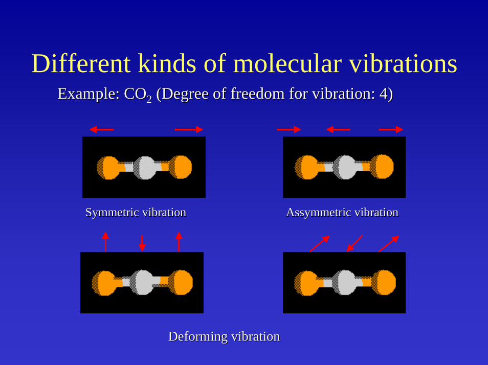
Different kinds of molecular vibrationsExampleExample: CO: CO22 ((DegreeDegree ofof freedom for vibrationfreedom for vibration: 4): 4)
SymmetricSymmetric vibrationvibration Assymmetric vibrationAssymmetric vibration
Deforming vibrationDeforming vibration
Lecture on atmospheric remote sensing [email protected]
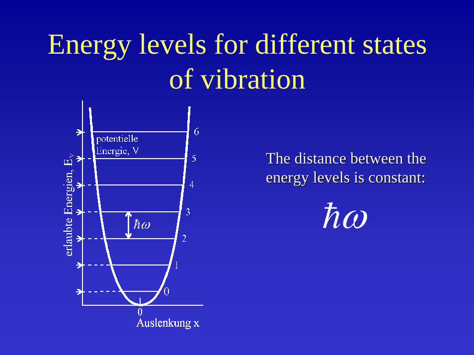
Energy levels for different statesof vibration
TheThe distancedistance between the between the energy levels is constantenergy levels is constant::
ω

Lecture on atmospheric remote sensing [email protected]
Energy levels for different statesof vibration
TheThe distancedistance between the energy between the energy levels are not constantlevels are not constant. For. Forincreasingincreasing vv thethe distancedistance decreasesdecreases..There exist onlyThere exist only aa limited numberlimited numberofof eneryg levelseneryg levels..
2
0 01 1( )2 2
⎛ ⎞ ⎛ ⎞= + − +⎜ ⎟ ⎜ ⎟⎝ ⎠ ⎝ ⎠
eG v v v xν ν

Lecture on atmospheric remote sensing [email protected]
Absorption cross section of the OClO molecule
0
2E-18
4E-18
6E-18
8E-18
1E-17
1.2E-17
1.4E-17
300 320 340 360 380 400 420 440Wavelength [nm]
Abs
orpt
ion
cros
s se
ctio
n [c
m²]

Lecture on atmospheric remote sensing [email protected]
250 300 350 400 450 600 650 7000
100200
Detection Limit
200 pptL=1km
1 pptL=16km
2 pptL=12km
20 pptL=12km
500 pptL=5km
5 pptL=5km
100 pptL=5km
200 pptL=5km
1 ppbL=5km
Phenol
Wavelength [nm]
04080
20 pptL=1km
50 pptL=1km
250 pptL=1km
para-Kresol
05
10
Toluol
01020
Benzol
0100200
IO
050 BrO
020 ClO
01
HCHO
0100 NO3
04
HONO
0
2NO2
048
SO2
0
4250 300 350 400 450 600 650
50 pptL=5km
σ'[1
0-19 c
m2 ]
O3
Solution:
-identification of different absorption processes by their spectral signature
=> Differential optical absorption spectroscopy (DOAS)
-consideration of scattering processes by broad band spectral structures, e.g. loworder polynomials

Lecture on atmospheric remote sensing [email protected]
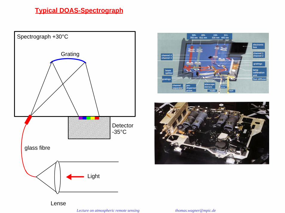
glass fibre
Spectrograph +30°C
Grating
Detector-35°C
Typical DOAS-Spectrograph
Light
Lecture on atmospheric remote sensing [email protected]
glass fibre
Spectrograph +30°C
Grating
Detector-35°C
Typical DOAS-Spectrograph
Light
channel 1channel 2
electronicbox
gratings
Sun diffuser
channel 4channel 3
beamsplitter
gratings
pre-disperserprism sun
channelseparator
Scannigmirror
nadir
telescopemirrors
595- 405- 240- 311-793 nm 611 nm 316 nm 405 nm
lampcalibrationunit

Lecture on atmospheric remote sensing [email protected]
Absorption spectroscopy
⎭⎬⎫
⎩⎨⎧
⋅⎟⎠
⎞⎜⎝
⎛+−⋅= ∫ ∑
l
si
ii dssII0
0 )()()(exp)()( λερλσλλ
Beer- Lambert-law :
σi: Absorption cross section of trace gas iρi: Concentration of trace gas iεs: Scatter coefficient
=> From the knowledge of the absorption cross section it is possible to determine the trace gas concentration
Optical depthOptical depth ττ

Lecture on atmospheric remote sensing [email protected]
Example: NO2 observation
0.E+00
2.E-19
4.E-19
6.E-19
8.E-19
250 300 350 400 450 500 550 600 650 700 750
Wavelength [nm]
abso
rptio
n cr
oss
sect
ion
[cm
²]
Typical wavelength window
l⋅⋅= ρστPath length: 6km
NO2 mixing ratio: 10ppb (parts per billion)
Air concentration: 2.9e19 molec/cm³
NO2 concentration: 2.9e11 molec/cm²
τ ≈ 0.07
=> I/I0 ≈ 0.93

Lecture on atmospheric remote sensing [email protected]
-also scattering reduces the measured intensity

Lecture on atmospheric remote sensing [email protected]
460 480 500 520 540
Wellenlänge [nm]
Inte
nsit
t I(
)
O3-Absorption
NO2-Absorption
Meßspektrum
'differentielle'optische Dichte
''ln0
σ⋅
⎟⎠⎞⎜
⎝⎛
=l
II
c
I’0
I
'σ
σ3
σ1
σ2
λ3λ2λ1
σdiff
Wavelength [arb. Units]
Cro
ss s
ectio
n [a
rb. U
nits
]

Lecture on atmospheric remote sensing [email protected]
0.96
0.99
1.02
400 300 200 100
pixel
atm
os. s
pekt
.
305 310 315
0.9998
1.0000
1.0002
resid
ual
wavelength [nm]
0.998
1.000
1.002
HCH
O
0.996
0.999
1.002
SO2
0.998
1.000
1.002
NO
2
0.998
1.000
1.002
O3
Example of a spectral analysis of O3, NO2, SO2, and HCHO in the polluted air of Heidelberg. The absorptions identified in the atmospheric spectrum (top trace) were: O3: 21.1 ± 0.5 ppb, SO2:0.64 ±0.01 ppb, and HCHO: 3.7 ± 0.1 ppb. The NO2 mixing ratio was not determined since this wavelength interval is not optimal for its analysis. The missing area around 312 nm was excluded from the analysis procedure.
Lecture on atmospheric remote sensing [email protected]
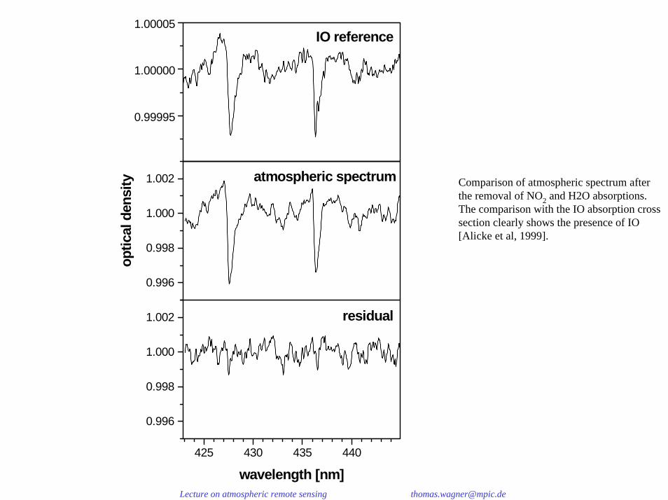
425 430 435 440
0.996
0.998
1.000
1.002
wavelength [nm]
residual
0.996
0.998
1.000
1.002
optic
al d
ensi
ty atmospheric spectrum
0.99995
1.00000
1.00005IO reference
Comparison of atmospheric spectrum after the removal of NO2 and H2O absorptions. The comparison with the IO absorption cross section clearly shows the presence of IO [Alicke et al, 1999].

Lecture on atmospheric remote sensing [email protected]
NO3 time series collected in the marine boundary layer of Mace Head, Ireland. The letters denote the origin of the observed air masses: A, Atlantic, P polar marine, EC, easterly continental, NC, northerly continental
[Allan et al, 2000].

Lecture on atmospheric remote sensing [email protected]
Catalytic ozone destruction mechanisms:
X + O3 → XO + O2
XO + O → X + O2
Net: O + O3 → 2O2
with:
X = OH, NO, Cl, Br

Lecture on atmospheric remote sensing [email protected]
Observation of Observation of volcanic emissionsvolcanic emissions
C. Kern, IUP HeidelbergC. Kern, IUP Heidelberg

Lecture on atmospheric remote sensing [email protected]
Lecture on atmospheric remote sensing [email protected]

Lecture on atmospheric remote sensing [email protected]

Lecture on atmospheric remote sensing [email protected]
Halogen compounds in coastal regions?
C. Peters, PhD-thesis, IUP Heidelberg

Lecture on atmospheric remote sensing [email protected]

Lecture on atmospheric remote sensing [email protected]

Lecture on atmospheric remote sensing [email protected]
Lecture on atmospheric remote sensing [email protected]

Lecture on atmospheric remote sensing [email protected]

Lecture on atmospheric remote sensing [email protected]
K. Hebestreit,K. Hebestreit,
PhDPhD--thesisthesis, IUP , IUP HeidelbergHeidelberg

Lecture on atmospheric remote sensing [email protected]
High High BrO coincides with low BrO coincides with low O3O3

Lecture on atmospheric remote sensing [email protected]

Lecture on atmospheric remote sensing [email protected]

Lecture on atmospheric remote sensing [email protected]
Long Path DOAS
-basic principle
-Long path DOAS (UV/vis/IR)
-instrumental improvements
-Specific applications
-white cell
-vertical profiles
-tomographic inversions
Lecture on atmospheric remote sensing [email protected]
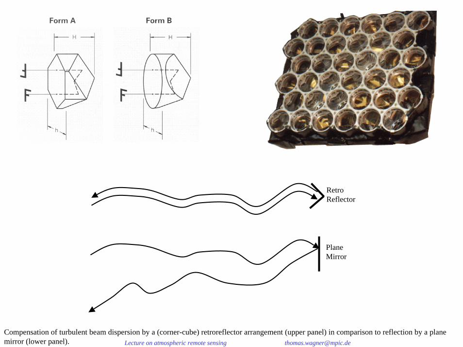
Retro Reflector
Plane Mirror
Compensation of turbulent beam dispersion by a (corner-cube) retroreflector arrangement (upper panel) in comparison to reflection by a plane mirror (lower panel).

Lecture on atmospheric remote sensing [email protected]
Lecture on atmospheric remote sensing [email protected]

Lecture on atmospheric remote sensing [email protected]

Lecture on atmospheric remote sensing [email protected]
J. Stutz, J. Stutz, PhDPhD--thesisthesis, IUP Heidelberg, IUP Heidelberg
Lecture on atmospheric remote sensing [email protected]

Lecture on atmospheric remote sensing [email protected]

Lecture on atmospheric remote sensing [email protected]
J. Stutz, J. Stutz, PhDPhD--thesisthesis, IUP Heidelberg, IUP Heidelberg

Lecture on atmospheric remote sensing [email protected]
R. Ackermann, R. Ackermann, PhDPhD--thesisthesis, IUP Heidelberg, IUP Heidelberg

Lecture on atmospheric remote sensing [email protected]
J. J. TschritterTschritter, , DiplomaDiploma--thesisthesis, IUP Heidelberg, IUP Heidelberg

Lecture on atmospheric remote sensing [email protected]
������������� ���������
� ������������������������������������������
������������������
��� ����� �������� ��
� ���� ���
����������� ����
! �"� �� �������#���������� ���
���������������$���������%������
�������� ���������&�����������
�������������������������������������
�������������������������'�(&������������������������������� )�
������������%������
����������
��������������������������������
������������������$���
�������
*+,-���������
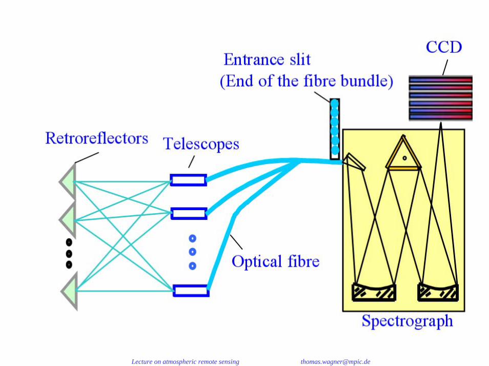
Schematic set-up of a DOAS system using a coaxial arrangement of transmitting- and receiving telescope in conjunction with a retro-reflector array [Geyer et al. 2001]. This type of set-up pioneered by Axelsson et al. [1990] has become the standard for artificial - light DOAS systems for research in the recent years.

Lecture on atmospheric remote sensing [email protected]

Lecture on atmospheric remote sensing [email protected]

Lecture on atmospheric remote sensing [email protected]
C. Hak, Dissertation, IUP Heidelberg, 2007C. Hak, Dissertation, IUP Heidelberg, 2007

Lecture on atmospheric remote sensing [email protected]
J. J. TschritterTschritter, , DiplomaDiploma--thesisthesis, IUP Heidelberg, IUP Heidelberg

Lecture on atmospheric remote sensing [email protected]

Lecture on atmospheric remote sensing [email protected]

Lecture on atmospheric remote sensing [email protected]
DOAS instrument used during theSOS field campaign in Nashville, TN, 1999, picture : Cathy Burgdorf, http://www.atmos.ucla.edu/~jochen/research/doas/DOAS.html

Lecture on atmospheric remote sensing [email protected]
Long Path DOAS
-basic principle
-Long path DOAS (UV/vis/IR)
-instrumental improvements
-Specific applications
-white cell
-vertical profiles
-tomographic inversions

Lecture on atmospheric remote sensing [email protected]
Lecture on atmospheric remote sensing [email protected]

Lecture on atmospheric remote sensing [email protected]
-Multi-Reflektions-System (White-Zelle):
Hohlspiegel
0.1 - 15 m
Lichtquelle& Spektrograph

Lecture on atmospheric remote sensing [email protected]
A. Geyer
Schematic optical set-up of the 'White' multi-pass system with a base path of 15 m as used during a field campaign in Pabstthum/Germany.
500 W Xe -arclamphouse
Quartz fibre withmode-mixer
Transferoptics
PC

Lecture on atmospheric remote sensing [email protected]
Schematic of the DOAS setup in the EUPHORE chamber in Valencia, Spain [Volkamer et al. 2002].

Lecture on atmospheric remote sensing [email protected]
Long Path DOAS
-basic principle
-Long path DOAS (UV/vis/IR)
-instrumental improvements
-Specific applications
-white cell
-vertical profiles
-tomographic inversions

Lecture on atmospheric remote sensing [email protected]
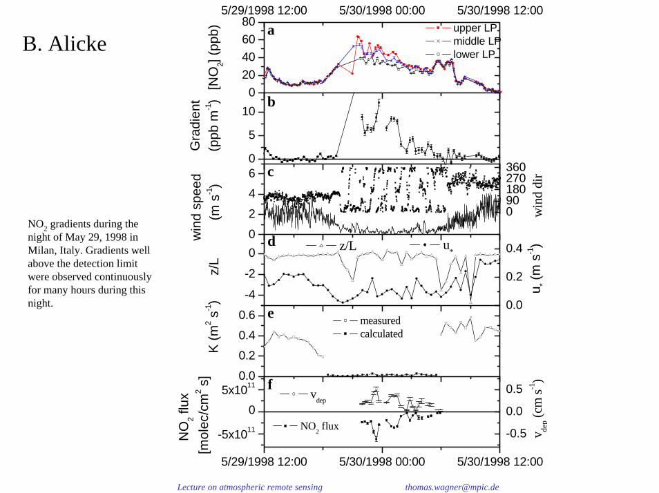
B. Alicke
DOAS
4 m
1.25 km
1.57 m
2.45 m
1.8 m
Sonic Anemometer
2.1m
Set-up of the experiment to measure gradients and fluxes of NO2 and HONO during the PIPAPO experiment. The DOAS instrument aimed sequentially at the three retroreflectors mounted on the tower at 1.25 km distance.
Lecture on atmospheric remote sensing [email protected]
020406080
5/29/1998 12:00 5/30/1998 00:00 5/30/1998 12:00
0.0
0.2
0.4
-4
-2
0
0.0
0.2
0.4
0.6
0
5
10
5/29/1998 12:00 5/30/1998 00:00 5/30/1998 12:00
-5x10¹¹
05x1011
-0.5
0.0
0.5
a
[NO
2] (p
pb) upper LP
middle LP lower LP
d u*
u * (m
s-1) z/L
z/L
measured calculated
e
K (m
2 s-1)
b
G
radi
ent
(ppb
m-1)
f
NO2 flux
NO
2 flu
x [m
olec
/cm
2 s]
vdep
vde
p (cm
s-1)
0
2
4
6 c
win
d sp
eed
(m
s-1)
090180270360
win
d di
r
B. Alicke
NO2 gradients during the night of May 29, 1998 in Milan, Italy. Gradients well above the detection limit were observed continuously for many hours during this night.

Lecture on atmospheric remote sensing [email protected]
0
1
2
35/29/1998 12:00 5/30/1998 00:00 5/30/1998 12:00
01002003004000.0
0.4
0.8
5/29/1998 12:00 5/30/1998 00:00 5/30/1998 12:00
-2x10¹⁰
0
2x10¹⁰
-0.5
0.0
0.5
0.00
0.03
0.06
-1
0
1
a
HO
NO
(ppb
) upper LP middle LP lower LP
c
NO
(p
pb)
b
gra
dien
t(p
pb m
-1)
e
HONO flux
HO
NO
flux
(m
olec
cm
-2 s
-1)
net vdep
vde
p (cm
s-1)f
d
[HO
NO
][N
O2]
HO
NO
corr
(ppb
)
B. Alicke
HONO gradients during the night of May 29. (a) shows the mixing ratios on the individual light paths (LP). The gradient is displayed in (b). To remove the influence of direct HONO emissions we calculated HONOcorr by subtracting 0.65% of the NOx(not shown here) from the HONO mixing ratios (d). The ratio of HONO to NO2 mixing ratios is displayed in (e). The fluxes and net deposition velocities is shown in (f)..

Lecture on atmospheric remote sensing [email protected]
J. Stutz
RTU 115mRTM 99mRTL 70m
DOAS Systems
WT 44mME 2m
6.1 km1.9 km750m
Setup during the TEXAQS 2000 experiment. Five retroreflector arrays were mounted at different distances and altitudes. The measurements weree performed by two DOAS instruments [Stutz et al, 2004].

Lecture on atmospheric remote sensing [email protected]
0 5 10 150
20406080
100120
altit
ude (
m)
0 5 10 15
2254
0 5 10 15
0042
0 5 10 15
0240
NO2 (ppb)
0 50 1000
20406080
100120
0 50 100 0 50 100 0 50 100
NO3 (ppt)
0 20 40 600
20406080
100120
0 20 40 60 0 20 40 60 0 20 40 60
O3 (ppb)
120
2032
J. Stutz
Vertical mixing ratio profiles during the night of 8/31 – 9/1 at four different times (noted on top of the graphs). The N2O5 mixing ratios shown are calculated from the steady state of measured NO2 ,NO3 , and N2O5 [Stutz et al., 2004].

Lecture on atmospheric remote sensing [email protected]

Lecture on atmospheric remote sensing [email protected]

Lecture on atmospheric remote sensing [email protected]

Lecture on atmospheric remote sensing [email protected]
Long Path DOAS
-basic principle
-Long path DOAS (UV/vis/IR)
-instrumental improvements
-Specific applications
-white cell
-vertical profiles
-tomographic inversions

Lecture on atmospheric remote sensing [email protected]
A. A. HartlHartl, Dissertation, IUP Heidelberg, 2007, Dissertation, IUP Heidelberg, 2007

Lecture on atmospheric remote sensing [email protected]
tomographic measurement setup during the BAB II campaign at the motorway BAB 656 between Heidelberg and Mannheim
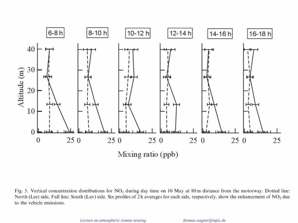
Lecture on atmospheric remote sensing [email protected]

Lecture on atmospheric remote sensing [email protected]
Modelled concentration distribution of NO2 and measurement setup
Measured (reconstructed) concentration distribution of NO2

Lecture on atmospheric remote sensing [email protected]
KaiKai--Uwe Mettendorf, Dissertation, IUP Heidelberg, 2006Uwe Mettendorf, Dissertation, IUP Heidelberg, 2006
Lecture on atmospheric remote sensing [email protected]

Lecture on atmospheric remote sensing [email protected]

Lecture on atmospheric remote sensing [email protected]
Measurement setup for the validation measurements

Lecture on atmospheric remote sensing [email protected]

Lecture on atmospheric remote sensing [email protected]

Lecture on atmospheric remote sensing [email protected]

Lecture on atmospheric remote sensing [email protected]

Lecture on atmospheric remote sensing [email protected]
Summary (I) Long Path (active) DOAS
-most direct application of the Lambert-Beer law
-long absorption path is needed to become sensitive even for small trace gas concentrations
-many trace gases were first observed by LP DOAS
-measurements also during night
-only the averaged trace gas concentration along the light path can be obtained (from simple LP DOAS)
-expensive and complicated instrumental set-up

Lecture on atmospheric remote sensing [email protected]
Summary (II) Long Path (active) DOAS
-recently many instrumental improvements were introduced, e.g. fibre optics, LED as light sources, which make instruments much cheaper and easier to operate
-many specialisations of LP-DOAS exist for specific applications:
-White (multi-reflection) system
-light paths at different altitudes
-balloon-borne reflectors
-tomographic inversions

Lecture on atmospheric remote sensing [email protected]

Lecture on atmospheric remote sensing [email protected]://www.lumileds.com/pdfs/techpaperspres/SID-BA-Paolini.PDF
Leuchtdichte von LEDs
Zum Vergleich:
Sonnenoberfläche1,5 x 10
9cd/m
2
Xenon Hochdrucklampetyp 4x 10
8cd/m
2
Glühdraht einer Glühlampe5 bis 35x 10
6cd/m
2
moderne Leuchtstofflampe0,3 bis 1,5x 10
4cd/m
2
Nachthimmeletwa 10
-11cd/m
2

Lecture on atmospheric remote sensing [email protected]
Lichtausbeute (Effizienz)Die Lichtausbeute ist ein Maß für die effektive Umwandlung elektrischer Energie in Lichtenergie. Die Effizienz der LED liegt zur Zeit bei bis zu 55 lm/W.

Lecture on atmospheric remote sensing [email protected]

Lecture on atmospheric remote sensing [email protected]


