

FINAL REPORT
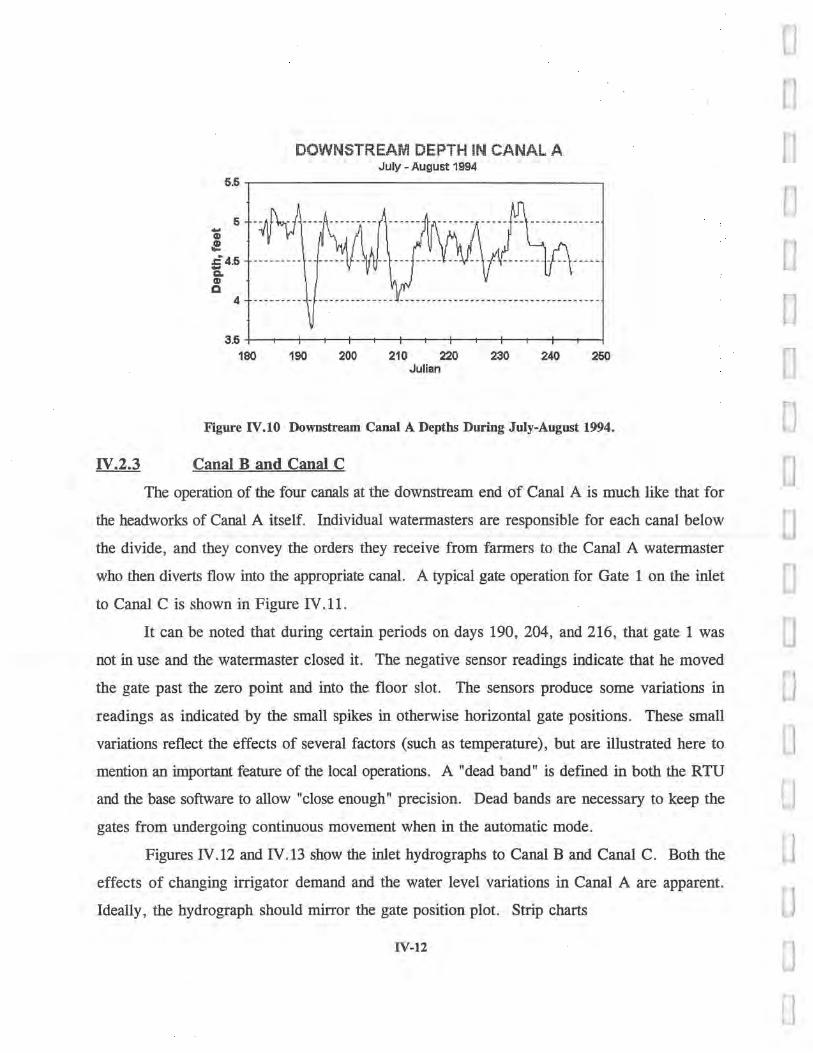
LOW COST ADAPTIVE CANAL AUTOMATION FOR CONSERVING
WATER AND MAXIMIZING DELIVERY SYSTEM FLEXIBILITY
This research was supported by the UNITED STATES DEPARTMENT OF THE INTERIOR, BUREAU OF RECLAMATION
Water Resources Research Laboratory Technical Service Center
Denvej,dColorado n er
Cooperative Agreement No. 1425-2-FC-81-18990 entitled
Water Conservation Innovative Technology Research - Irrigation Water
Water Technology and Environmental Research (WATER) Project No. WS032
Submitted by
Wynn R. Walker Blair L. Stringam
Department of Biological and Irrigation Engineering Utah State University
Logan, Utah 84322-4105
October 1994

r.
r. r, r, r. r, u r. r, v r r, C
ii
u u

FINAL REPORT
LOW COST ADAPTIVE CANAL AUTOMATION FOR CONSERVING
WATER AND MAXIMIZING DELIVERY SYSTEM FLEXIBILITY
This research was supported by the UNITED STATES DEPARTMENT OF THE INTERIOR, BUREAU OF RECLAMATION
Water Resources Research Laboratory Technical Service Center
Denven, (fol orado
er Cooperative Agreement No. 1425-2-FC-81-18990 entitled
Water Conservation Innovative Technology Research - Irrigation Water
Water Technology and Environmental Research (WATER) Project No. WS032
Submitted by
Wynn R. Walker Blair L. Stringam
Department of Biological and Irrigation Engineering Utah State University
Logan, Utah 84322-4105
October 1994

CONTENTS Page
ACKNOWLEDGEMENTS ......................................iv ABSTRACT............................................... v NOTATIONS .............................................. v TABLES .................................................A FIGURES................................................ vii
Section a
I EXECUTIVE SUMMARY ................................. I.1
II INTRODUCTION ............... .....................H.1 II.1 BACKGKOUND ..................................II.1 II.2 PROJECT CONCEPT ............................... II.2 II.3 RESEARCH OBJECTIVES AND SCOPE .................. II.3 II.4 EXPERIMENTAL DESIGN ........................... IIA
III INSTRUMENTATION ... ............................... III.1 III.1 SYSTEM HARDWARE ............................. III.1 III.2 CONTROLLER .................................. III.3 III.3 RADIO SYSTEM ................................. III.5 IIIA SENSORS ..................................... III.6 III.5 CONTROL AND INTERFACE WIRING .................. III.7 III.6 HARDWARE INSTALLATION ........................ III.9 III.7 GATE MECHANIZATION ........................... III.9
IV FIELD IMPLEMENTATION .............................. IV.1 IVA DESCRIPTION OF FIELD SITE ....................... IV.1
IV.1.1 Location and Setting ...................... IV.1 IV.1.2 Conveyance Losses ....................... IV.2 IV.1.3 Characteristics of the Canal A Inlet ............ IVA IV.1.4 Characteristics of the Canal A Channel .......... IV.5 IV.1.5 The Canal C, West Ditch and Pump Ditch ........ IV.6 IV.1.6 Canal B Headworks ...................... IV.8
IV.2 FIELD OPERATIONS .............................. IV.9 IV.2.1 DMAD Reservoir ........................ IV.9 IV.2.2 Upstream and Downstream Conditions in Canal A .. IV. 10 IV.2.3 Canal B and Canal C .................... IV.12 IV.2.4 Canal A Losses ......................... IV.14
IV.3 GENERAL OBSERVATIONS ........................ IV.17
ii

VSOFTWARE .........................................V.1 V.1 BASE STATION SOFTWARE ......................... V.2
V.1.1 General Program Description ...................... V.3 V.1.2 Program and System Configuration .................. VA V.1.3 Monitoring and Control ......................... V.7
V.1.3.1 RTU Data Displays .................... V.7 V.1.3.2 Monitoring System Control Prompts ........ V.10
V.1.4 Output ................................... V.12
V.2 SOFTWARE FOR THE REMOTE TERMINAL UNITS ........ V.16 V.2.1 Modes of Operation ........................... V.16 V.2.2 RTU Logic ................................. V.18 V.2.3 Testing ................................... V.20
V.3 SIMULATION SOFTWARE .......................... V.22 V.3.1 Software Configuration ......................... V.22 V.3.2 Input Data ................................. V.23 V.3.3 Evaluation of Channel Resistance .................. V.24 V.3.4 Evaluation of Channel Seepage .................... V.26
VI TECHNOLOGY TRANSFER .............................. VIA VIA ADVERTISING CANAL AUTOMATION ................. VIA
VI.1.1 Preparing Visual Aids for Demonstrations ........ VIA VI.1.2 Presentations and Demonstrations .............. VI.2
VI.2 LOCAL TRAINING ............................... VIA VI.3 PUBLICATIONS ................................. VI.5
VII CONCLUSIONS AND RECOMMENDATIONS ................. VH.1 VIIA CONCLUSIONS ...... VII.1 VII.2 RECOMMENDATIONS ........................... VII.3
APPENDIX I DESCRIPTION OF THE CANAL SIMULATION MODEL ... A-1 A.1 BACKGROUND ..................................A-1 A.2 MODEL DESCRIPTION AND APPLICATION ............... A-1 A.3 TECHNICAL FEATURES ............................ A-2 A.4 MODEL LIMITATIONS ............................. A-3 A.5 REFERENCES ...................................A-3
iii
ACKNOWLEDGEMENTS f Funding for this study was provided under Bureau of Reclamation Cooperative 0 Agreement No. 1425-2-FC-81-18990, Utah Agricultural Experiment Station Project AES803,
and by the Delta Canal and Melville Irrigation Companies.
The authors wish to thank the following individuals for their cooperation during this P g study: Mr. Clyde Bunker, President of the Melville Irrigation Company and the DMAD Reservoir Company; Mr. Kenneth Fowles, past President of the Delta Canal Company; and Mr. Dean Anderson, Secretary of the DMAD Reservoir Company. Personnel from the Technical Service Center and the Utah Projects Office of the Bureau of Reclamation provided valuable technical assistance throughout the project, and the authors appreciate their insights. Contracting Officer's Technical Representatives were Danny L. King and Philip H. Burgi.
Special appreciation is due Mr. Leon Smith, watermaster for the Melville Irrigation Company and operator of Canal A. Without his cooperation and support, this project would not have been possible.
51
iv
ABSTRACT
Canal automation was investigated in Central Utah to determine if such technology could be used to conserve water and to improve flexibility in responding to demands. Operational and seepage losses in the test canal over the previous 5 years averaged more than 10% of diversions. In 1993, local officials reported losses had been reduced 55% and attributed the reductions to the automation. The value of the water "saved" on the local rental market was twice the total cost of the automation. In only July and August 1994, the savings nearly equaled the cost of the system again. Watermaster travel was reduced by 400 miles per week and allowed a fourfold increase in the frequency of system adjustments. Based on these findings, it is concluded that: (1) canal automation can result in substantial water conservation; (2) remote manual control followed by full automatic control can result in significant increases in the frequency and reliability with which canal systems respond to irrigator demands, yielding more flexible and timely service; and (3) there are substantial and measurable benefits to both the irrigation company (or district) and their field personnel from reduced travel expense and better, more accurate flow regulation.
List of Key Words: Canal Automation, Canal Systems, Demand Scheduling, Flow Regulation, Instrumentation, Irrigation, Controllers, Sensors, Telemetry, Water Conservation.
NOTATIONS
This manuscript is submitted for publication with the understanding that the United States Government is authorized to reproduce and distribute reprints for governmental purposes.
The views and conclusions contained in this document are those of the authors and should not be interpreted as necessarily representing the official policies, either expressly or implied, of the U.S. Government.
The United States Government does not endorse products or manufacturers. Trade or manufacturer's names appear herein only because they are considered essential to the object of the document.
v

D
TABLES
Number Page
III.1 Base Station Components and Costs ...................... III.1 III.2 Repeater Station Components and Costs .... ............... III.2 III.3 Components and Costs of the DMAD System ................ III.2 IIIA Components and Costs of the Canal B System ................ III.2 III.5 Components and Costs of the Canal C Automation ............. III.3
A

FIGURES
Fizure Pa.e III.1 Schematic Diagram of Spring Return Water Level and Gate
Position Sensors ....................................... III.6 III.2 Schematic Diagram of the Weighted Pulley Water Level Sensor .......... III.6 III.3 Wiring Diagram of the Control Interface ........................ III.8 III.4 Canal Side RTU in the Canal A System ....................... III.10 III.5 Overall View of the Canal C Gate Structure ..................... 111. 11 III.6 Close-up View of the Canal B Gate Mechanism ................... 111. 11
IV.1 Location and Setting of the Field Site .......................... IV.1 IV.2 Historic Canal A Losses as a Percent of Diversions ................. IV.2 IV.3 Historic Canal A Losses in Acre-Feet Per Year .................... IV.3 IVA Canal A Cross-Sections .................................. IV.6 IV.S Canal C Weir Rating Curve ............... ... ............ IV.7 IV.6 DMAD Elevations in July-August 1994 ......................... IV.9 IV.7 DMAD Gate Positions in July-August 1994 ..................... IV. 10 IV.8 Canal A Inlet Hydrograph During July-August 1994 ................ IV.11 IV.9 Canal A Inlet Depths During July-August 1994 ................... IV.11 IV. 10 Downstream Canal A Depths During July-August 1994 .............. IV. 12 IV.11 Canal C Gate 1 Positions During July-August 1994 ................ IV. 13 IV. 12 Canal C Inflow During July-August 1994 ...................... IV. 13 IV. 13 Canal B Inflow During July-August 1994 ...................... IV. 14 IV. 14 Cumulative Inflow-Outflow in Canal A During July-August 1994 ........ IV. 16 IV. 15 Cumulative Losses in Canal A During July-August 1994 ............. IV. 16
V.1 Monitor Display Map in Base Station Software ..................... V.1 V.2 Opening Screen of Base Station Software ......................... V.3 V.3 Configuration Screen for Software and System Setup ................. V.5 VA The Monitor Screen at the Base Station .......................... V.8 V.5 Gate Opening Target Screen ............................... V.12 V.6 Graphics Plot of Monthly Inflow to Canal A ..................... V.13 V.7 Daily Canal Structure Hydrograph for Canal A Inflow ............... V.14 V.8 Numerical Display of Monitoring Data for Canal A Inflows ............ V.15 V.9 Flow Chart of the RTU Programming ......................... V. 19 V.10 Inflow and Outflow to Canal A from July 15th to August 14, 1995 ........ V.23 V.11 Canal A Inflow Minus Outflow During the Period of July 15th through
August 14, 1995 ...................................... V.24 V.12 Comparison of Measured and Simulated Upstream Depths in Canal A
as a Function of Channel Resistance ........................... V.25 V.13 Comparison of Measured and Simulated Downstream Depths in Canal A
Under Various Manning n Values ............................ V.25
vii j

V.14 Comparison of Measured and Simulated Upstream Depths in Canal A Under Different Seepage Rates .............................. V.26
V.15 Comparison of Measured and Simulated Downstream Depths in Canal A Under Different Seepage Rates .............................. V.26
V.16 Estimated Seepage Loss Rates in Canal A During the Simulation Period ..... V.27
VI.1 Photo of Robogate Showing a Full Scale Automatic Canal Gate with Upstream and Downstream Water Level Sensors, Gate Position Sensor and Complete RTU ..................................... VI.3
VI.2 The Robogate Monitoring Display ............................ VI.3

SECTION I
EXECUTIVE SUMMARY
This investigation examined the use of canal automation to conserve water within canal
networks and to improve their flexibility in responding to irrigator demands. Emphasis was given
to approaches that are particularly applicable to small- and medium-sized irrigation projects,
although the results can be applied to systems of any size. The small and medium systems dominate
irrigation in the West but have not historically benefited from the application of canal automation.
An increasing number of these irrigation systems are moving toward demand scheduling as irrigators
seek more timely delivery service. At the same time, irrigation companies and districts are
increasing the competition for water with municipalities, industry, and environmental concerns.
Agriculture must make a better justification for its use of water by maximizing efficiency. Under
these circumstances, canal automation offers new opportunities and solutions which many irrigation
projects will need.
Two irrigation companies in central Utah, the Delta Canal Company and the Melville
Irrigation Company,' approached the Bureau of Reclamation and Utah State University in 1991 to
automate their "Canal A." Canal A is a common canal which conveys water from DMAD Reservoir
through a six mile earthen canal to a "divide" where the headworks of each company are located.
The division is comprised of two major canals, one minor canal, and a pumping station serving a
fourth canal. The two companies share the O&M of Canal A.
Operational losses over the five years preceding this investigation had averaged more than
ten percent. In terms of the local water market, this loss amounts to as much as $200,000 per year.
Irrigators under both companies have demanded more flexible delivery schedules which has made
it increasingly difficult to manage the canal. From early discussions with the companies, a three-
way partnership evolved to implement and test the concept of automation in Canal A. The two
r 1 I.1 Both of these companies are organized as mutual ditch companies administered by a five member board of directors elected by the stockholders. These two companies, together with two others, operate a consolidated "water office." The water office is managed by a full time person responsible for record keeping, procurement, and disbursements.
0 I-1

I 0 companies contributed $10,000 toward the cost of sensors, telemetry, and computer equipment.
They also assumed full responsibility for mechanizing the reservoir and canal gates. The Bureau
of Reclamation provided funding and technical review of the project. Utah State University
designed and installed the monitoring and control system, and then provided O&M support during
the 1993 and 1994 irrigation seasons.
Two aspects of the project were given priority--low cost and adaptability. Costs were
minimized by coordinating monitoring and control from an IBM compatible pc computer at the
company office. A portable base station was also installed in the watermaster's2 truck so he could
monitor and regulate the system away from the water office. Water level and gate position sensors
were designed and built at the University, and a datalogger manufactured by a Utah company was
used for the canal-side monitoring system and gate controller.' The irrigation companies
mechanized existing reservoir and canal gates by adapting small electric motors to the gate frames.
Power for all canal gates was provided by a local ac line, but the reservoir gates had to be powered
by a solar panel and battery. Communication between the field sites and the base station was
facilitated by four-watt hand-held UHF radios adapted to the system through RF modems provided
by the datalogger supplier. The total cost of automating Canal A, including labor but excluding
software development, was about $42,000. There are 11 mechanized gates with position sensors,
10 water level sensors, three RTU's, and one telemetry repeater station.
The project included four phases: (1) instrumentation, which is discussed in Section III; (2)
field implementation and testing (Section IV); (3) software development (Section V); and (4)
technology transfer and training (Section VI).
The primary instrumentation devices associated with canal automation were the sensors that
measure and transmit water levels and gate positions. At the beginning of this investigation the
I.2 The designation of field personnel who operate the canals on a daily basis is "watermaster." Other terms such as "ditch rider" are in common use elsewhere.
I.3 The assembly of communication equipment, processor, datalogger, gate controller, etc. that must be located adjacent to the canal gates or monitoring stations is generally referred to as a "remote terminal unit" or RTU. The RTU abbreviation is used throughout this report and specific mention of individual components will only be made when they are of particular interest.
I-2
N
0

average cost of commercial sensors exceeded $600 per unit. At these rates, sensors would have
exceeded 50% of the hardware costs of the project. To determine if sensor costs could be reduced
by simplification and in-house manufacture, USU designed and built a self-contained sensor based
on a spring-wound pulley equipped with a rotational potentiometer. All gates and water level
positions were equipped with these for the first three months of the field investigation. An
evaluation revealed that the sensors were adequate for gate positions but not for water levels. A new
version for the water levels was designed using a simple weighted pulley equipped with a rotational
potentiometer. The old sensors at the water stage locations were replaced with the new version and
the results were adequate for the remainder of the investigation.
By the end of the project, the cost of commercial sensors had declined to $350-$400 per unit.
New devices such as those based on ultrasonic measurements are now available for about the same
cost. Thus, the need for substantial efforts to reduce sensor costs under future canal automation
projects is significantly reduced or eliminated.
The other key elements of the instrumentation package were the datalogger and telemetry
system. Prior to the initiation of this study, USU and the Utah Projects Office of Reclamation had
discussed the feasibility of using the Campbell Scientific, Inc. CRIO datalogger as the basic element
of the RTU.4 To convey sensor data to the base station as well as instructions from the base station
back to the datalogger, the Campbell Scientific RF95 modem and Motorola p50 hand-held radio
were used. The first CRIO's purchased for the project only had 2k bytes of programmable memory.
While the programming of the unit was efficient, the maximum number of instructions limited the
code in its error handling. However, midway through the project, modifications were made to the
CRIO that doubled the programmable memory to 4k bytes. Towards the end of this study the
memory was increased again to 8k bytes. These memories were found to be quite capable of
handling typical gate control algorithms. Thus, with the increased memory, the CRIO is an
effective RTU controller capable of gate control and data acquisition for installations of less than
6 gate structures. Larger systems could multiple CRIO's or migrate to a larger capacity controller.
I.4 Neither USU nor Reclamation specifically endorse any commercial product. The mention of the company name and product designation are to provide an accurate description of the system.
01 I-3
I

fl
m
The software to control and manage the system was comprised of two parts: (1) software for
the pc microcomputer at the base station needed to coordinate system-wide management; and (2)
software in the CR10 needed to interrogate sensors, convert readings, and operate the gate
structures. The development of the base station software was complicated by the problems of
commanding and interrogating the CR10's. Campbell Scientific provided their own software, but
this was not adequate for systems management. Consequently, a program was written based
originally on Campbell's own internal logic to connect the base station to the remote units. This
program was then supplemented with an interactive interface, input and output routines, graphics,
and control logic so the watermaster could operate Canal A from either the base station or from a
companion unit in his truck. This software is currently being adapted to other canal automation
projects in Utah.
The RTU software underwent several major revisions. Like the base station software,
considerable experimentation was necessary to develop a package that would work effectively under
the Canal A conditions. Most of the work involved programming to control gate movements.
Three gate control options were programmed. The first we have called "remote manual gate control"
in which new gate settings and a control flag are sent to the RTU from the base. The RTU then
activates a power switch on the appropriate gate motor, checks to verify that the gate is moving,
monitors the gate position until it is within a tolerance interval of the target, shuts off the gate motor,
and resets the control flag.
The second gate control option has been labeled "remote manual discharge control" in which
the base sends revised gate positions based on discharge targets. Under this option the operator
specifies a gate flow target to the base station software which then uses current water level and gate
position readings to compute a new gate position. The operation at the RTU level is therefore the
same as in remote manual gate control.
The third control option is "remote automatic discharge control." Under this option, the base
sends the RTU's targets for all gates and sets an automatic flag. The RTU then continuously
computes revised gate positions using adjacent water level readings and internal gate ratings and
adjusts the gate positions as necessary to maintain the flow targets. During automatic control the
RTU functions independently of the base station. Automatic control is only terminated whenever
I-4

a control error occurs or when the automatic flag is deactivated by the base. This option can be
applied to either the upstream or downstream water level control if necessary and can be repeated
during each base poll of the remote units to yield a step-wise approximation to full automation.
Field implementation of the system involved automating the canal, monitoring the system,
controlling the gates, and performing maintenance. As expected, the most important lessons evolved
from field applications--sensor designs were revised, software logic was modified and adapted, and
equipment problems were identified and resolved. But more interesting, the impact of the
automation on local canal management was observed. In 1993 (and independently of either USU
or the Bureau of Reclamation) the water companies reported that losses in Canal A had been reduced
55% and attributed the reductions to the automation. The value of the water "saved" on the local
rental market was twice the total cost of the demonstration project. In 1994 the losses were again
less than one-half the pre-automation loss rates. In only July and August of 1994, the savings
nearly equaled the cost of the system again.
. These were not the only benefits. The watermaster reported that the automation reduced his
travel by as much as 400 miles per week for a savings of $116 per week. He maintains that the
frequency of system adjustment to irrigator demands is now four times the rate prior to automation.
s He also reports, however, that the system has not saved him as much time as he would have
expected. Time historically spent driving to the stations is now required to monitor and adjust
sensor calibrations, check flow readings, and perform system maintenance. Some of this effort will
be reduced as improvements in sensors and telemetry are made and the need to satisfy USU data
requirements is ended.
The effective transfer of this technology to irrigators was recognized from the beginning of
the project. USU personnel attempted to include the local watermaster in each step of the field
implementation and a number of hardware and software changes were made during the project at
his suggestion. Every effort was made to explain what steps were being taken, why they were
important, and possible problems he may observe. Regular visits were made to the site to support
him. At the end of the project the watermaster was operating the system without USU guidance,
I.5 This is perhaps only an indirect benefit of the automation made possible by the ease and precision of system management.
I-5

performing maintenance, isolating and fixing problems, and evaluating the results of his
management.
In addition to local technical support and training, USU and Reclamation staff participated
in the Utah Water User's Workshop where presentations were made to more than 75 water users and
state agency personnel. A field day was held at Delta to give irrigation companies and districts in
Utah a chance to see an automated canal in operation and discuss applications in their systems. The
results of these activities have been quite remarkable. There are more than five irrigation companies
already proceeding with similar plans and have asked USU and Reclamation for assistance. Plans
are being discussed to apply this technology to local river systems as well.
In describing and discussing canal automation with irrigators in Utah, it is apparent that they
anticipate a somewhat different benefit of automation than what has been reported elsewhere. They
are primarily interested in the capability to remotely monitor conditions at a select number of critical
points. They are less interested in monitoring every site because the costs outweigh the perceived
benefits. For reservoirs or diversions some distance from the irrigated area, the capability for remote
manual gate or discharge control is also an attractive option. Again, however, remote control of
every structure is considered too costly.
Fully automatic canal-side water level or discharge control does not yet generate significant
interest. Most irrigation company or district personnel presently lack sufficient confidence in remote
control devices to trust them in an unattended mode. Most irrigation systems in Utah use separate
flow measurement structures downstream of regulating gates and therefore lack the calibrations of
the gates needed for remote automatic discharge or water level control. It is interesting that even
at Delta with two years of experience with the Canal A system, full automatic control is not a high
priority. Yet, with the increasing frequency of gate adjustments now being made to accommodate
irrigator demands, the transients in Canal A are more substantial, causing more variations in the
downstream canals.
At least part of the limitations with which this project demonstrated full automatic control
was a lack of operational time and the difficulty in calibrating the gates. After completing the
implementation and debugging the software and hardware, there simply wasn't sufficient time for
the system to earn credibility beyond monitoring and remote manual control. Projects such as this
will need to develop longer-term technical support for future implementations.
I-6

The ability to remotely monitor and control conditions of difficult-to-manage facilities or
those some distance away are the primary perceived benefits of low-cost and adaptive canal
automation. Remote automatic discharge control will have important benefits in the fixture but will
require more experience with the elements of automation. There are three important conclusions
from this study: (1) canal automation, which includes advanced capabilities for monitoring and
accounting, can result in substantial water conservation; (2) remote manual control followed
eventually by full automatic control can result in significant increases in the frequency and reliability
with which canal systems respond to irrigator demands, thereby leading to more flexible and timely
service; and (3) there are substantial and measurable benefits to both the irrigation company (or
district) and their field personnel from reduced travel expense and better, more accurate flow
measurement.
I-7

r ~i n
a
0
n
n
fl
0
0 0
0 n
0
u 0

SECTION H
INTRODUCTION
II.1 BACKGROUND
The performance of existing irrigation systems can usually be achieved with better and
more responsive management and control, which in turn may require improvements in auxiliary
functions -- such as flow measurement and scheduling. Performance can be characterized by
both efficiency (water conservation) and effectiveness (the system's ability to respond faster and
more reliably to irrigator demand). To improve system performance, both efficiency and
effectiveness must be optimized. This can best be achieved through improved water
management (the strategy for water control, distribution, allocation, and scheduling) and
improved water control (the regulation of water levels and flows).
The conditions which affect water movement in a canal change unpredictably in time and
space: the capacity and response of some canals where moss or aquatic weeds are a problem
may decline significantly in a period of weeks; seepage losses vary from reach to reach and as
water levels fluctuate; and the demand for water is dependent on weather variability.
Historically, these problems have been partially ignored until they became critical. Many canals
simply operate "full"; fields are irrigated the same way each time, and deliveries are made
according to a schedule whether they need water or not. Consequently, it is not uncommon for
a 30 to 40% loss of water to occur from the stream diversion to the field outlet due to seepage,
spills, unregulated turnouts, and poor measurement. Additionally, because of uncontrolled
tailwater or deep percolation, equivalent losses are common at the field level. Without a much
more rigorous approach to management and control, these losses cannot be reduced.
For many years engineers, agronomists, and economists examining the production
associated with water at the farm level have argued for more flexible and demand-based delivery
schedules. How this might be accomplished without complete redesign of an existing system
has been difficult to answer, and perhaps canal automation has become the most feasible
alternative. Canal automation can be implemented in several different ways, but if it is to
improve both control and management, it must include two capabilities: (1) it must provide the

canal manager and operator with real-time information about water levels and flows, and (2). it
must be capable of remote manual or automatic gate regulation.
If timely information on water levels, discharges, and structural settings are key elements
in improving the performance of the canal network, then the question arises as to how it should
be controlled and managed. Thereafter, the questions of what data are really necessary, how
to collect and transfer data to the decision maker, and how to derive the right decisions from the
information require consideration. For a more advanced level of management and control to be
successful, data acquisition, transmission, and analysis should follow a more intensive, ~y
computer-assisted methodology and be largely accomplished by stand-alone electronic devices.
Otherwise neither the farmers, the canal companies or districts, nor the state and federal
agencies have the time, interest, or funding to increase the level of information use. Finally,
the question of whether or not this technology can be cost-effectively adapted to existing canal }
systems and integrated with local water management practices needs to be addressed. ~f
This investigation examines the use of canal automation technologies to conserve water ,
within the distribution systems, primarily within small- and medium-sized irrigation projects.
These systems dominate irrigation in the West but have not historically benefited from the
application of canal automation. Irrigation companies and districts are in increasing competition
for water from municipalities, industry, and environmental concerns and must make substantially
better use of water. Canal automation offers new opportunities and solutions to these problems.
I1.2 PROJECT CONCEPT
The premise of this investigation was that water management and control in an irrigation
delivery system can be more efficient and effective if the acquisition, transfer, and interpretation
of field data along with the implementation of regulation decisions are adaptive and automated.
The concept of "adaptive" canal automation is important in two ways. Most irrigation
schemes cannot afford to replace existing facilities with devices engineered for automation.
Thus, canal automation's first requirement is that it be adaptable to existing canal structures.
Since it is infeasible to apply automation to every structure and device in an irrigation system,
the canal automation must also be adaptable to operational practices already in use. This is not
to assert that canal automation should not induce changes in existing practices. Such changes
11-2

will necessarily occur. It does argue that automation must be a integral part of water
management in the larger context and then be flexible enough to evolve with and in response to
other irrigation practices.
The third aspect of adaptive automation is that it provide for periodic assessment of the
state of the irrigation delivery system within the more general framework of "supervisory
control." Control of irrigation systems is often described as "downstream" if the system
automatically adjusts for withdrawals like a municipal water supply, or as "upstream" or
"supervisory" if water management is coordinated centrally and routed to outlets in response to
requests for water. Most irrigation management in canals is based on the "supervisory"
approach and is most effective when the interface with irrigators is well coordinated. A
supervisory control system is typically management oriented in the central office and control
oriented in the field. If the supervisory control system can adapt to varying field conditions,
the ability of central management to plan and execute system-wide water distribution is
substantially improved. At first glance, few non-automated systems would appear to exhibit any
capability toward adaptive control. However, many field personnel develop considerable skill
in reacting to the dynamic changes in an irrigation project.
II.3 RESEARCH OBJECTIVES AND SCOPE
The principal objective of this investigation was the development of an integrated system
of software, data acquisition, and control systems which can be applied selectively and
retroactively in a wide range of canal distribution systems to conserve water and increase
delivery flexibility.
Automation technology has a distinct diminishing return when applied to an existing
irrigation delivery network. For the locations that are difficult to manage and operate, or are
remote, automation allows the canal managers and operators the advantage of more precise local
control, reduced travel to the remote sites, and the capability to make more daily adjustments.
For other stations that are close, or operate simply, the benefits of automation are substantially
less and perhaps infeasible. Thus, in most cases, implementing high-technology management
and control systems throughout a canal system would be infeasible, unrealistic, and unnecessary.
II-3

Under this concept, canal automation offers three services (in descending order .of
importance): (1) monitoring, (2) remote manual gate and discharge control, and (3) remote
automatic discharge or water level control.
IIA EXPERIlVIENTAL DESIGN
The work plan for this investigation involved four tasks: (1) instrumentation; (2)
software development; (3) field implementation, evaluation, and demonstration; and (4)
technology transfer.
There were two purposes of an instrumentation phase. Initial installations will be
infeasible if equipment costs are not minimized. Irrigators are generally less aware of recurring
costs for maintenance and replacement than they are up-front expenses. Initial decisions
concerning new and untried technologies are often based on equipment and installation costs
outlays rather than costs associated with reliability and labor savings which become significant
long-term issues. Sensors and RTU's are expensive pieces of equipment. Thus, the first
purpose of an instrumentation phase was to determine if less expensive controller and datalogger
equipment would work satisfactorily as an RTU, and if locally fabricated sensors would prove
reliable and accurate. The second purpose of an instrumentation phase was to demonstrate that
water conservation and reliable, flexible water scheduling depend heavily on timely, accurate
information.
In addition to the important need for field testing of any new concept, the field
implementation phase of this project was aimed at two important problems that are in the minds
of the irrigators: (1) can canal automation cost-effectively improve a canal company's (or and
irrigation district's) ability to supply water on-demand, and (2) will automation reduce
conveyance losses. These two questions are related, and the selection of an area to implement
and test canal automation was based on a local interest to address both questions simultaneously.
During the last 10 years, the stockholders of the Delta Canal Company and the Melville
Irrigation Company of Delta, Utah have wanted a more "on-demand" operation--the willingness
to wait for water has diminished substantially. The older farmers attribute this to the impatience
of the younger generation. But one thing is obvious, as the system has tried to be more
responsive, the losses have increased significantly. When canals can be well regulated and the
II-4
measurement accurate, the losses can be reduced substantially. Of course one might argue that
the "losses" were mostly administrative, but to the users the losses are real since they cannot be
sure they received the water. The 11 % losses in 1991 occurred in a relatively dry year. The
7,000 acre-feet of loss from the main supply canal to the companies (Canal A), was worth about
$210,000 in the local rental market, or in terms of water at the field level, about one irrigation
on the lands served.
The development of microcomputer software to connect the management function of a
central office to the control locations along a canal system was a major focus of this project.
The principle software objective was to develop an integrated supervisory control and a RTU
software package that would allow a canal manager to make the same judgements from the office
that he or she would make from the field, but with substantially more precision and on a more
periodic basis. A critical function of the software was to indicate how the canal and its
structures were changing, and what effects these changes were having on the operation of the
canal.
Canal automation which is adaptive and low cost must be operated, maintained, replaced,
and updated by the water users themselves. Pressing concerns over water supplies for non-
agricultural uses suggest that canal automation be adopted and applied to many systems in Utah
and throughout the West. It is important, therefore, that canal automation technology be
"transferred" to local interests. Federal and state resources are inadequate to provide extensive
technical support to the number of irrigation companies and districts that should eventually
implement canal automation.
II-5


SECTION III
INSTRUMENTATION
III.1 SYSTEM HARDWARE
A base station at the headquarters of the irrigation companies and three field stations
comprised the monitoring and control system for the automated canal. The headquarters site
consisted of a pc computer connected via modem to a radio which could call, interrogate, and
command the field stations. The field stations included: one at the Canal A outlet from DMAD
Reservoir, one at the headworks of Canal B serving most of the Delta Canal Company, and one
at the headworks of Canal C supplying the Melville Irrigation Company. The equipment
required at the remote site included a site controller (Campbell Scientific CR10), radio modem,
radio, interface electronics (connecting the controller to sensors and gate actuators), water level
sensors, and gate position sensors. The site at DMAD Reservoir could not be contacted directly
by the base station and a repeater station was located near the Delta Municipal Airport. The
individual components and costs for each station are listed in Tables III.1 - 111. 5.
TABLE HIJ Base Station Components and Costs.
[7Quantity Cost Item Cost
1 ea 486 PC $2,700
1 ea Base Radio
/Modem
$950
1 ea Antenna $200
50 ft Radio Cable $50
20 ft RS232 Cable $20
Total Cost 1 $3,920
A major goal of the design in this canal automation system was to use low-cost equipment
that could be acquired locally. A small inventory of parts was acquired to replace some
components while others could be obtained within one to two days.
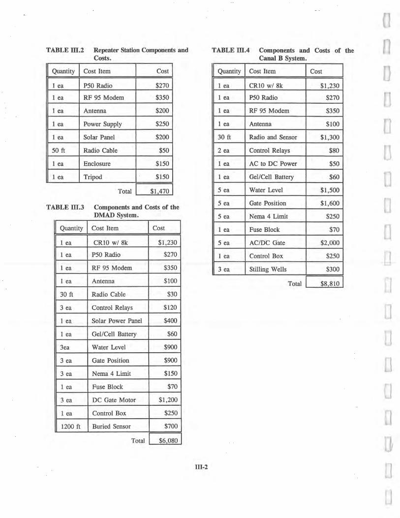
TABLE M.2 Repeater Station Components and Costs.
Total $1 470
TABLE M.3 Components and Costs of the DMAD System.
Quantity Cost Item Cost
1 ea CR10 w/ 8k $1,230
1 ea P50 Radio $270.
1 ea RF 95 Modem $350
1 ea Antenna $100
30 ft Radio Cable $30
3 ea Control Relays $120
1 ea Solar Power Panel $400
1 ea Gel/Cell Battery $60
3ea Water Level $900
3 ea Gate Position $900
3 ea Nema 4 Limit $150
1 ea Fuse Block $70
3 ea DC Gate Motor $1,200
1 ea Control Box $250
r1200 ft Buried Sensor $700
Total $6 080
TABLE MA Components and Costs of the Canal B System.
Quantity Cost Item Cost
1 ea CR10 w/ 8k $1,230
1 ea P50 Radio $270
1 ea RF 95 Modem $350
1 ea Antenna $100
30 ft Radio and Sensor $1,300
2 ea Control Relays $80
1 ea AC to DC Power $50
1 ea Gel/Cell Battery $60
5 ea Water Level $1,500
5 ea Gate Position $1,600
5 ea Nema 4 Limit $250
1 ea Fuse Block $70
5 ea AC/DC Gate $2,000
1 ea Control Box $250
3 ea Stilling Wells $300
Total $8 810
III-2
Quantity Cost Item Cost
1 ea P50 Radio $270
1 ea RF 95 Modem $350
1 ea Antenna $200
1 ea Power Supply $250
1 ea Solar Panel $200
50 ft Radio Cable $50
1 ea Enclosure $150
1 ea Tripod $150

TABLE III.S Components and Costs of the Canal C Automation.
FQuantity I Cost Item Cost
1 ea CR10 w/ 8k Memory $1,230
1 ea P50 Radio $270
1 ea RF 95 Modem $350
1 ea Antenna $100
30 ft Radio Cable $30
3 ea Control Relays $120
1 ea AC to DC Power 50
1 ea Gel/Cell Battery $60
3ea Water Level Sensors $900
3 ea Gate Position Sensors $900
3 ea Nema 4 Limit Switches $150
1 ea Fuse Block $70
3 ea AC/DC Gate Motor $1,200
1 ea Control Box $250
1200 ft Buried Sensor Cable $700
3 ea Stilling Wells $300
Total $6130
In the arrangement with the canal companies, the company personnel were asked to
mount motors on the control gates and run power to all parts of the system. The watermaster
also participated in the installation of the system.
USU developed control and management software, and designed and installed the central
communication site, site controllers, control interface systems, and radio communication
systems. This type of arrangement benefitted the project since the canal companies were able
to determine many of the problems and perform repairs as required.
III.2 CONTROLLER
The controller chosen for this project was the Campbell Scientific CR10. This device was
selected since it was locally manufactured, extensively used, had a good reputation for
III-3

[r7
reliability, had on-board surge protection, and a radio communication system that was readily
available. The CR10 came from the factory with 12 single-ended or 6 double-ended analog
inputs. The input accepts a maximum voltage of 2.5 Vdc. While this limited voltage span was
initially a concern, it was found that input could be resolved to 333 µvolts. In other words, a
sensor with a 10 foot span would have a resolution of 0.016 inches or 0.41 millimeters. The
maximum span used on the sensors in this project was 7 feet so the resolution was reduced to
0.01 inches or 0.28 millimeters. The system used 4-to-20 milliamp sensors and dropped the
output signals across a 125 ohm precision resistor to match the 2.5 Vdc input.
The CR10 also had 8 discrete outputs which were used for controlling gate motors, and
had additional features such as programmable analog outputs and pulse counters.
The CR10 came with limited memory but could be modified to double or quadruple
the memory for a cost of $50 to $300 depending on the number of units modified. The CR10
demonstrated sufficient programming capability for the functions required for this project.
Additional functions could be included if required. The CR10 units used in this project had
either the 4K or 8K memory modifications. A 4K unit was programmed to control 5 structures [ J
but was later replaced by an 8K memory device which allowed a better implementation of sensor
calibration coefficients.
In addition to controlling the gates, the CR10 also performed checks for common f 1 problems that occurred such as water levels becoming too high or too low, gates drifting from U
the last set position, gates not moving when required to move, bad sensors, and large unplanned 0 changes in measured values. The CR10 performed all programmed functions with little
difficulty. Most of the problems and malfunctions that occurred with these controllers were due 0 to programming mistakes or problems with the power supplies.
There are a number of other controllers available for canal automation which have been
tested elsewhere. Considering the cost and capabilities, the CR10 suited this project very well.
The CR10 proved to be one of the more reliable components of the monitoring and control 10 system. And judging from the programming capabilities of the CR10, nearly any control routine
implemented in other controllers could be implemented in the CR10. a
III-4 0
I

III.3 RADIO SYSTEM
The radio system consisted of a Motorola p50 radio and a Campbell Scientific RF95
modem. This system was designed with the dual capabilities of communicator for the CR10 and
as a repeater station. Each RTU station had a unique radio address which it responded to during
a polling event initiated by the base station. If an individual RTU station was also to act as a
repeater, the radio address sent from the base had two parts, the address of the local RTU
followed by the address of the end-of-line station it is repeating to. A chain of up to 255 RTU
stations could be linked as repeaters for the end-of-line station. This feature made this kind of
system more efficient and economical than many.
The station at the Canal A headworks was not radiometrically visible from either the base
station or the other two field stations. Consequently, a repeater site consisting of a modem and
radio was required.
An interesting variation of the repeater concept in this project was the use of the base
station by the watermaster. The mobile base installed in his truck lacked both the height and
the quality of the headquarters base and the field stations. As a result, there were times when
he could not poll one or more of the stations. On his own initiative he programmed the address
sequence to include the headquarters base and found that it would act as a repeater for the rest
of the system. This improved the capability of the mobile base, but it created a periodic conflict
between the mobile and headquarters bases when they were both attempting to poll the field
sites.
This communication system worked well initially. But as the system was used, more and
more communication problems were encountered. Problems were isolated by selectively
replacing the CR10, the RF95 modem and the p50 radios. In nearly every case, the p50 radios
were the cause of the problem. The watermaster in charge of maintaining the system was able
to isolate and change the failed radios using spare units but the frequency of the failures was
troubling. Following the 1994 irrigation season, the authors consulted a number of local and
industry radio specialists and discovered that voltages above 10 volts tend to degrade the final
drive transistors in these particular radios. Since the power supplies to the RTU systems were
common to each component and set at about 13 Vdc, future field installations will have to be
modified to supply the radios from a special circuit to correct this problem.
III-5

IH.4 SENSORS
When this project was first considered, a major concern was the cost of the water level
and gate position sensors. The initial estimate for these sensors was over $15,000--about one-
third of the total equipment and installation cost. After considering several different kinds of
sensors, a potentiometer-based sensor was designed and used to measure both water levels and
gate positions. The total cost for these sensors was approximately $6,600. These sensors were
a return spring type. They worked well for gate position measurement, but they did not respond
properly for water level measurements. In order for the water level sensing to be more accurate
the sensor was modified for a weighted float and pulley design. Schematics of both sensor
designs are shown in Figures. III.1 and III.2. When 10 or more of these sensors are
manufactured, each individual sensor costs $300. If more than 20 sensors are manufactured,
the cost is reduced to $250 to $280 per sensor.
Figure M.1 Schematic Diagram of the Figure H1.2 Schematic Diagram of Spring Weighted Pulley Water Level Return Water Level and Gate Sensor. Position Sensor.

The potentiometer is connected to a 4-to-20 milliamp current loop device to allow for
better signal transmission. The 4-to-20 milliamp device is an industry standard which is used
for the following reasons:
1. The sensors in the current loop are immune to and not corrupted by external
noise.
2. Isolation can be provided for individual sensors such that when one sensor is
exposed to a surge, other sensors will not experience the same surge.
3. Resistance changes that may occur due to cable deterioration or corrosion in
connections will not interfere with the sensor calibration.
III.5 CONTROL AND INTERFACE WIRING
Despite a well-designed control system or expensive components, system parts will
eventually fail and require replacement. Since these systems would be located in rural locations,
the components used in this project were common devices that could be easily obtained in a
short period of time. The control interface was also designed so that a problem could be
determined and corrected with little difficulty by the watermaster.
The CR10 did not have enough power to operate the relays that turn gate motors on and
off, so opto-isolators were used to energize the control relays. These devices also isolated the
CR10 from the control interface so that it could be protected from surges that may propagate
through the control interface circuit. The interface system used standard 12 Vdc relays with
three-pole double throw contacts. All fuses were common automotive glass fuses, and most of
the parts could be acquired at electrical supply shops or hardware stores. A schematic of one
of the wiring diagrams for the system is shown in Fig. III.3
The wiring required for the relays was incorporated into a PC board thus eliminating
installation wiring time and allowing modular construction. If a control problem arose in the
interface system, a relay board could be removed and replaced simply by disconnecting a few
wires. By designing in this manner, downtime was minimized and the electrical expertise was
III-7

DMA Gate 1 wring 1z we gra.
Figure M.3 Wiring Diagram of the Control Interface.
reduced. This also limited the need for extensive wiring since the majority of the wiring was
contained within the printed circuit board.
The control interface circuit was also designed with redundant control features. Control
systems are not totally infallible, so these features were required for protection. In the event
of a lightning strike or a mistake on the part of the site operator, for instance, the computer may
operate the site in such a way that damage would occur to system components. For example,
a lightning strike could disrupt or confuse the controller to such an extent that it may attempt
to drive the gate all the way to the end of the gate movement limits. If some sort of protection
is not designed into the system, the gate motor may burnout, the gate and gate frame may be
damaged, the movement mechanism may be ruined, or (if fortuitous circumstances happen) the
gate fuse will burnout.
Limit switches were installed on each gate and connected to the control interface wiring.
These switches will not allow the gate to be driven too far in one direction. If the gate is driven
to the end of its movement, the gate will trip a limit switch. At this point, the circuit is opened,
III-8

and the gate ceases to operate. This wiring safety is also beneficial if the person operating the
gate is not paying attention and drives the gate to its high- or low-limit.
Another feature incorporated into the interface system was a normally closed down-relay
contact in the up-relay energizing circuit and a normally closed up-relay contact in the
down-relay energizing circuit. This redundant feature was included to ensure that the gate could
be driven in only one direction at a time. If the up-relay was energized, the normally closed
contact in the down-relay energizing circuit would be opened, and the down-relay could not be
turned on while the up-relay was being operated. The relays and relay control circuits were
incorporated into a printed circuit board to speed installation and repairs.
Manual switches were also included in the control system. The CR10 was isolated from
the system when the switch was set to manual. Isolating the controller ensured that control
adjustments were not made when an operator made a manual adjustment. Also, in the event that
the operator made a mistake when making a manual adjustment and caused the controller to
respond in an undesirable manner, the controller could be switched to manual until the proper
corrections were made. As mentioned earlier, lightning may cause the controller to perform in
a manner that is not compatible with the control system. At this point, the controller could be
retired via the manual auto switch.
IV.6 HARDWARE INSTALLATION
A major cost of a control system is the cost of installation. For this project it was
estimated that hardware installation at Canal A and Canal C each required 10 person-days.
Installation of hardware at Canal B (including the West Canal and Pump Ditch) required
approximately 12 person-days. Figure III.4 shows a photo of a completed RTU.
IIIJ GATE MECHANIZATION
The responsibilities for designing, building, and maintaining the gates, gate motors and
power supplies were assumed by the canal companies. This significant involvement by the
companies and allowed USU concentrate on software and the RTU. The gate mechanization was
accomplished with exceptional skill and, except for minor problems, the gates worked well.
III-9

Figure MA Canal Side RTU in the Canal A System.
The outlet gates at DMAD Reservoir were motorized with do motors powered by a solar
panel and automobile battery. The gates were previously moved with a portable hydraulic pump
system or hand crank. The companies mounted the electric motor over the gate stems and
connected the motor to the gate sprocket with a chain. USU equipped the gates with limit
switches and connected the motor switches to the RTU. This installation worked very well
throughout the study. The motors had more than enough power, and the battery was maintained
by the solar panel.
The mechanization of the Canal B, Canal C, and West Ditch gates used the same scheme.
Figures III.5 and II1.6 give two views of the gate structures. The gates were rectangular slide
gates normally lifted or closed by manually turning a large wheel on a frame above the gates.
The motors for these gates were mounted on the gate frame itself and turned the gate by a chain
connecting a motor gear to a larger sprocket bolted to the existing wheel assembly. The motors
were ac/dc motors connected to a 110 ac power line. It was substantially harder for the
tit-to

¢w T

911
companies to mechanize these gates, and in the end the motors were slightly too small. In the
future the canal companies plan to replace all of these motors, although they partially resolved
the problem by changing gear ratios.
In the early stages of the gate mechanization, the companies asked about the speed
with which the drives should raise and lower the gates. The authors felt for this pilot study, it
would be best to move the gates slowly in order to reduce motor size, as well as allow the RTU
to control gate position more precisely. Thus, all of the gates were set to move at about 0.1 feet
per minute. 0
11
III-12

Data Display - Press F1 - Ganal A at DMAD F2 - Ganal B Offtake F3 - Ganal G Offtake R — Restore Display
SECTION IV
FIELD IMPLEMENTATION
IVA DESCRIPTION OF FIELD SITE
IV.1.1 Location and Settine
Figure IV.1 Location and Setting of the Field Site.
Figure IV.1 is the monitoring map from the base station software and illustrates the
location and setting of the field site near Delta, Utah. The Delta Canal Company and the
Melville Irrigation Company divert water from DMAD Reservoir into a common canal named
"Canal A." Canal A is an earthen conveyance six miles long which follows the southern bank
of the Sevier River. DMAD Reservoir is one of two regulating reservoirs at the terminus of the
Sevier River. It serves a smaller reservoir, Gunnison Bend Reservoir, 10 miles downstream
from which the Abraham and Deseret Irrigation Companies divert irrigation water. The name
"DMAD" is the abbreviation for Delta, Melville, Abraham, and Deseret, the four mutual ditch
companies that own and operate the dam.
IV-1

12
10
i►
X 9192
All of the DMAD irrigation companies are mutual ditch companies administered by five
person boards of directors elected annually by the stockholders. The boards elect a president,
and the four presidents constitute the board of directors for the DMAD Reservoir Company.
The four presidents elect the DMAD president.
The four companies, together with the Intermountain Power Association and the Central
Utah Canal Company, form the Sevier Bridge Reservoir Company. This company owns and
operates the Sevier Bridge Reservoir located about 30 river miles above DMAD Reservoir--the
main supply facility to the Delta area. The entire system operates under an on-demand supply
strategy.
IV. 1.2 Conveyance Losses
Year
Figure IV.2 Historic Canal A Losses as a Percent of Diversions
Figure IV.2 shows the historic losses in Canal A as a percentage of totol diversions. To
illustrate the importance of these losses, it is first necessary to note that water is "rented" among
both irrigators within an individual company and between companies. In 1994, the rental price
per acre-foot of water exceeded $40. The losses, therefore, are not only a concern in crop
IV-2

-6000 d
a)
It
4000
-1 2000
A
production but also a concern in allocatng water among farmers. The value of the historic losses
shown above exceeds $200,000 annually.
Since the early 1950's, all of the companies have undertaken extensive lining projects.
In fact, Canal A is one of the few remaining unlined main canals. Despite the linings, the
differences between the inflows at the canal headworks and farm deliveries remains above 30%.
These "losses" are comprised of both seepage and administrative loss, i.e., water that cannot be
accounted for by the measurement system and water given or "not counted" by the watermasters
during periods of regulation. Local measurements in the mid-1980's showed that seepage losses
were approximately 5 %. Thus, substantial reductions in conveyance losses have to be achieved
by better management and control.
Year
Figure IV.3 Historic Canal A Losses in Acre-Feet Per Year.
Figure IV.3 shows the same information as Figure IV.2 except in terms of "volume of
losses. " One observation is that as the companies have tried to deliver water into their canal
headworks on more of a demand basis, the losses have increased substantially.
IV-3
U If the 1994 rental prices were to apply over the period shown above, the 28-year
economic loss would be about $160,000 per year, and the average over the last eight years
would be $250,000 per year. One can easily see the monetary incentive for the irrigators in the
Delta, Utah area to conserve water.
IV. 1.3 Characteristics of the Canal A Inlet
The headworks of Canal A are located in the west leg of the DMAD dam. Three 4 by
6 foot rectangular slide gates are mounted on a 30 degree incline with their invert located at
4848 feet MSL. Three rectangular box culverts convey the water through the dam and release
the water vertically through a manifold stilling basin at the head of the canal. About 200 yards
downstream, the flow is measured in a 15 foot rectangular flume.' The floor of the flume is
located at an elevation of 4846.60 feet MSL. The flume was designed to operate primarily in
the submerged flow regime, so water level measurements are made upstream and downstream
of the flume. The flume calibration that has been established over the years is:
iNE 85.602 * qI - H ) 1.62
a b
1 - S 1.3230.11 . to 1-S
gtu 17- S
in which Q is the flume discharge in cfs, Ha and Hb are the upstream and downstream depths
respectively in feet, and S is the submergence, Hb/Ha. When the value of S is less than 0.789,
the flume operates in a free flow regime described by:
Q - 36.294 * Ha 62
IV.1 In 1965, G.V. Skogerboe began the development of the "cutthroat" flow measuring flume. After developing and testing a theory, a field site was set up at the inlet of Canal A to verify the theory under field conditions. It measures 65 feet in length, has a 3:1 converging inlet, a 30 foot rectangular throat, and a 3:1 diverging outlet. Results of the field tests indicated that the stability of the exit flow was not good and laboratory tests were repeated resulting in a design with a 6:1 outlet and no throat section, thus the term "cutthroat."
IV-4
X 0 0
I Cl
X
if

The calibration for the reservoir gates is not satisfactory. There appear to be conditions
when the hydraulics approximate a sluice gate and other times when they behave like submerged
orifices. An approximate equation was developed from a limited appraisal of the monitoring
data:
Q - C . 4.0 . G, g(EL-48 -H )
in which Q is the gate flow in cfs, G,, is the gate opening in feet, EL is the water level in
DMAD reservoir (4800 feet), Ha is the upstream flume reading and Cd is a discharge coefficient
defined as:
C = 0.98 - 0.1.Go
This rating is used by the watermaster to make relative changes in the Canal A flow.
After the flow through the flume has stabilized, minor adjustments are made to the gate openings
to arrive at the desired flow.
IV.1.4 Characteristics of the Canal A Channel
In the fall of 1993 a survey of Canal A was made to determine bed slope and cross-
section. The slope was determined by surveying the elevations along the canal. It was found
that the elevation of the gate inverts at Canal B were 4842.82 feet MSL. The distance between
the inlet flume and the Canal B gates was 32,100 feet (6.08 miles). The average canal slope was
therefore 0.0001178 feet per feet.
Three cross-sections were surveyed along the canal. These are shown in Figure IVA.
When the canal depth at the lower end near the Canal B gates is five feet, the storage volume
in the canal is about 200 acre-feet. A one foot change in the canal water level elevation
corresponds to a volume change of about 40 acre-feet. This is an important feature of the canal.
For instance, in early August 1994 the demands on Canal A were about 200 cfs. Using only
the storage volume in the top one foot of the canal, these demands could be satisfied for more
than two hours without any release from the reservoir. Since the time required for a flow
change at the reservoir to reach the divide is about 2 hours, this means that the watermaster can
IV-5

10
y as 8 w E 0 V 0 In 5
0 U. M 4 CL d O
2 U
CANAL A CROSS-SECTIONS
-- - - - - - - - - - - - - - - - - - - - - - - - - - - - - - - - - - - - - - - - - - - - - - - - - - - - - -- - -- --
-®- Sta 1- Sta 2 --r-- Sta 3
--= ----- -------------------------------------------~ ̀-------
---------<-->---,----------------------------- --------------
0 10 13 1 39 43
Distance From North Bank, feet
Figure IV. 4 Canal A Cross-Sections.
supply demands into either company system as soon as they occur. Put another way, using the
storage volume of the canal with automation to regulate flows brings the supply point of the
Canal A system more than 6 miles closer to the irrigators. Without automation, the watermaster
must wait for flows to reach the divide before supplying the demands.'
IV. 1.5 The Canal C, West Ditch and Pump Ditch
At the downstream end of Canal A there are four canals. Canal B serves the
Delta Canal Company. Canal C, West Ditch and the Pump Ditch serve the Melville Irrigation
Company. All of the gates at the headworks of these canals are vertical rectangular slide gates,
three feet wide and about five feet high.
The three Canal C gates and the. West Ditch gate operate in a submerged condition and
are calibrated as follows:
IV.2 Since the operators do not need automation to use the canal storage in this manner, it can be argued that it is an indirect benefit of automation. However, there is substantial effort involved in stabilizing large, flat canals like Canal A. Only automated systems provide gate operations that are sufficiently frequent and precise that operators have confidence in being able to return the canal to a stable condition in a short period of time.
IV-6

Q - 0.73 Go * 3.0 g(FI -Hb )
in which Q is the discharge in cfs, G,, is the gate opening in feet, and Ha and Hb are the upstream
and downstream heads on the gates. This equation is used directly for West Ditch
measurements.
About 50 yards below the Canal C gates is a broadcrested weir or ramp flume. The
calibration of the weir is shown in Figure IV.5
CANAL C WEIR RATING 300
250
200 m
150 t cs
p 100
50
0
----------------------------------- -------------------------I
0 0.5 1 1.5 2 2.5 3 Head On Weir, feet
Figure IV. 5 Canal C Weir Rating Curve.
The pump lift is comprised of two pumps which can be operated together and
independently. A simple stage discharge relationship on the pump outlet defines the flows into
the pump ditch. This relationship is as follows;
Q = 12 cfs if 1.25 < Ha < 2.2
Q=14 cfs if2.4<Ha <2.6
Q = 24 cfs if Ha > 2.7
IV-7

IV.1.6 Canal B Headworks a Canal B diverts water from Canal A through five three foot rectangular slide gates, four
of which are mechanized and equipped with position sensors. After early discussions with the
watermaster, it was concluded that the fifth gate would not be used. The headworks structure
is somewhat unusual in that a concrete floor extends about 4 feet downstream of the gates
causing the gates to behave like sluice gates rather than submerged orifices. Attempts to
calibrate these structures have been complicated since none of the standard orifice or sluice gate
equations seemed to work. After some trial and error, the following relation was found;
Q - 0.73 * 3.0 * G * 2g-(H - G ) o a a
where Q is the gate flow in cfs, G,, is the gate opening in feet, and Ha is the head level on the _
upstream side of the gates. (~
About 200 feet downstream of the gates the flow is measured by a 12-foot Parshall Flume
which has the following rating:
Q - 34.56. Hal .51
in which Ha is the upstream head in the flume. In June of the 1994 season, the demands on the
Canal B system were unusually high and the flume became submerged. The design of the a
monitoring system had not anticipated this, and as a result, there were no measurements on the
downstream depth. The irrigators made adjustment to their records using measurements from
downstream offtakes, but the monitoring system was only able to evaluate the flows through the
gates. To get the high demand through the gates, the watermaster also opened the fifth gate.
Thus, neither the flume nor the monitoring system on the gates were giving accurate totals.
Because the problems of calibrating a control gate has generated an important conclusion
in this study with respect to adapting automation to existing systems, further discussion on this
subject will be left to a later section.
IV-8

IV.2 FIELD OPERATIONS
DMAD RESERVOIR STAGE July - August 1994
~, 68 d w 66 0 64 CD 62
2 60 Y
N 58
W 56
54 0 -062
W s0
---------
----------------------------------------------------
--------------------------- ----------------------------
--------------------------- ---------------- -- ---- ------------
180 190 200 210 220 230 240 260 Julian Date
Figure 11V.6 DMAD Elevations in July-August 1994.
IV.2.1 DMAD Reservoir
In order to illustrate the operation of the Canal A implementation in 1993 and 1994,
monitoring data from the July-August period of 1994 were converted from the raw data files to
spreadsheet files and plotted.
Figure IV.6 shows the water level in DMAD Reservoir. There are two things that
complicate the operation of Canal A inherent in the reservoir stage. First, the reservoir is
actually operated under the direction of the Sevier River Commissioner. Water is transferred
from Sevier Bridge Reservoir by the Commissioner after consulting with all four local
companies. Whenever there is a problem anticipating irrigator demand or the Commissioner and
the watermasters do not communicate accurately, DMAD Reservoir fluctuates. Since the flows
into Canal A respond to these fluctuations, the watermaster has to adjust gate settings
periodically to compensate. Secondly, neither the Delta Canal Company nor the Melville
Irrigation Company have winter storage rights in DMAD. They must therefore empty the
reservoir prior to November 1st of each year. This process begins in August, and thus Canal
A operations during the second half of the year have to be made when the reservoir level will
be trending downward.
IV-9
DMAD GATE OPENINGS July - August 1994
2
1.5
m c ~ 1 N Q 0 N
8 0.5
r^J
-~------ {` - - - - - - - - - - - - - - -~. - -- -
04- 180 190 200 210 220 230 240
Julian Date
Gate 1 Gate 2 ... Gate 3
Figure IV.7 DMAD gate positions in July-August 1994.
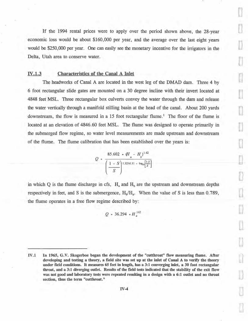
IV.2.2 Upstream and Downstream Conditions in Canal A
Figure IV.7 shows the gate positions at the Canal A headworks. Adjustments are made
in response to changing water levels in Canal A, increasing or decreasing demands on the
system, and adjusting for DMAD Reservoir levels. The results of the reservoir level
fluctuations and the gate adjustments are reflected in the Canal A inlet hydrograph shown in
Figure IV. 8.
The variability of this hydrograph is an important reason to incorporate remote automatic
control in the daily operations of Canal A. Even though the canal volume is large, these
fluctuations migrate downstream and complicate the management of the divide gates to the Canal
B, Canal C, and West Canals. For instance, the water levels in the upstream and downstream
ends of Canal A are shown in Figures IV.9 and IV. 10. The upstream water levels follow the
hydrograph as one would expect. The downstream levels reflect not only the transients
migrating along Canal A but also the fluctuations associated with flow management into the
company canals.
IV-10

3.5
3
2.5
1
0.5
CANAL A INLET DISCHARGE July - August 1994
300
250 w U
e200 IA i N
15 150 H 0
100
50 TITITITITITI i L1 180 190 200 210 220 230 240 250
Julian Date
Figure 11V.8 Canal A Inlet Hydrograph During July-August 1994.
UPSTREAM DEPTH IN CANAL A July - August 1994
-------------------------
- - - - - - - - - - - - - - - - - - - - - - -
It
---------------------------- \ -_
------- ------- - ------------------------------------ - /_ -
180 190 200 210 220 230 240 Julian Date
Figure IV.9 Canal A Inlet Depths During July-August 1994.
IV-11
r
a 7
DOWNSTREAM DEPTH IN CANAL July - August 1994
0
u A
11 a 7
•J 9 u
It
I ZUV Z10 ZZV Z3V Z4V Zou Julian
3.5 180
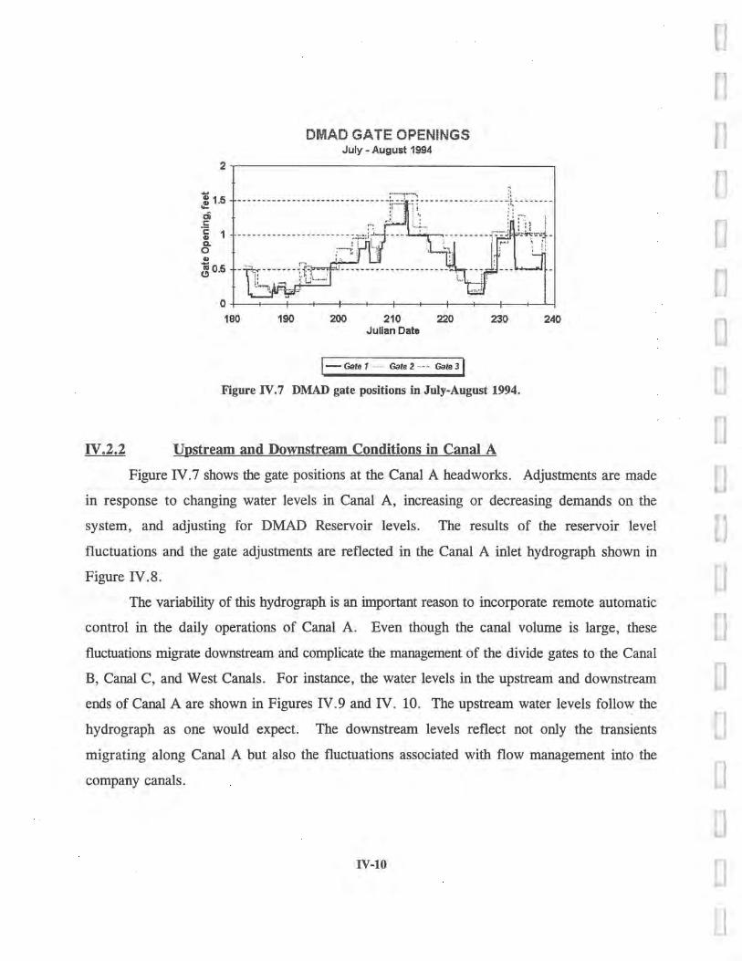
Figure IV.10 Downstream Canal A Depths During July-August 1994.
IV.2.3 Canal B and Canal C
The operation of the four canals at the downstream end of Canal A is much like that for
the headworks of Canal A itself. Individual watermasters are responsible for each canal below
the divide, and they convey the orders they receive from farmers to the Canal A watermaster
who then diverts flow into the appropriate canal. A typical gate operation for Gate 1 on the inlet
to Canal C is shown in Figure IV. 11.
It can be noted that during certain periods on days 190, 204, and 216, that gate 1 was
not in use and the watermaster closed it. The negative sensor readings indicate that he moved
the gate past the zero point and into the floor slot. The sensors produce some variations in
readings as indicated by the small spikes in otherwise horizontal gate positions. These small
variations reflect the effects of several factors (such as temperature), but are illustrated here to
mention an important feature of the local operations. A "dead band" is defined in both the RTU
and the base software to allow "close enough" precision. Dead bands are necessary to keep the
gates from undergoing continuous movement when in the automatic mode.
Figures IV. 12 and IV. 13 show the inlet hydrographs to Canal B and Canal C. Both the
effects of changing irrigator demand and the water level variations in Canal A are apparent.
Ideally, the hydrograph should mirror the gate position plot. Strip charts
IV-12

G 20
CANAL C GATE 1 OPENING July - August 1994
1.2
1
0.8 d w 0016
0.4 CL 0 0.2
0
-02
----------------------
I
------- iln-_ ---- -------- - - --- F ----------- - ------ --- ------- --- -------- - -- ------------------------
180 190 200 210 220 230 240 260 Julian Date
Figure IV. 11 Canal C Gate 1 Positions During July-August 1994.
CANAL C FLOW July -August 1994
100
80
-------------------------------
0 180 190 200 210 220 230 240 260
Julian Date
Figure IV. 12 Canal C Inflow During July-August 1994.
IV-13

CANAL B OUTFLOW July - August 1994
200
w 150 V
04- 180 190 200 210 220 230 240 250
Julian Date
Figure IV. 13 Canal B Inflow During July-August 1994.
recording the flume and weir heads are maintained by the two companies but their flow records
show only daily averages. As a result, it has not been possible to compare flow hydrographs
before and after the automation of Canal A. However, the authors have seen the strip
recordings and qualitatively judge that there is more variance in the hydrographs after
automation than before. Figures IV. 12 and IV. 13 indicate that Canal A is more responsive to
irrigator demands, but the quality of service may be poorer.' Again, the remote automatic
control would improve the stability of the canals without impacting the flexibility.
IV.2.4 Canal A Losses
The water rights of the two companies are defined at the Canal A flume. The flume is
actually under the supervision of the Sevier River Commissioner, and he maintains a recording
of the upstream and downstream heads and then calculates the flow allocated to the two
companies. The Canal A watermaster maintains water level sensors in the same stilling wells
for the Canal A monitoring system. The differences between what the River Commissioner
IV.2 The Canal B watermaster often asks the Canal A watermaster for additions and subtractions of as little as 1 or 2 cfs when the total flow in the canal is as high as 200 cfs. Consequently, part of the variance problem is that all the watermasters are using the flexibility of the Canal A automation.
IV-14

charges the companies and what they record as flows entering the four canals diverting from
Canal A are the losses.
The irrigation companies report that 1993 losses were about 3,300 acre-feet. The losses
from 1985 through 1992 averaged nearly 6,300 acre-feet. Both the watermaster and the DMAD
secretary have stated that the Canal A monitoring capability provided by the project was
substantially responsible for the lower losses. The value of this water on the 1993 local rental
market was $90,000. No attempt has been made to evaluate these figures using the monitoring
data from 1993. Setting up the system and correcting equipment problems left large gaps in the
electronic record, but as a rule the flume and weir measurements agree closely with the
companies' data.
At the time of this report, the companies had not yet released their 1994 loss figures.
The DMAD secretary told the authors that he expected the losses to be as low as reported for
1993.
For the purposes of this report, the data in Figures IV. 8, IV. 11, IV. 12 and hydographs
for the West Ditch and the Pump Ditch can be used to estimate losses in July and August 1994.
Figures IV. 14 and IV. 15 show two views of these results. Figure IV. 14 shows the cumulative
into and out of Canal A in July and August as measured by the monitoring system. At the end
of August, the total losses were about 960 acre-feet out of nearly 20,000 acre-feet diverted into
Canal A. This is a 4.8% total loss, or a savings of 900 acre-feet over the average value of the
last eight years.
Figure IV. 15 shows how the cumulative loss plots over the two month period. During
these two months, the average losses occurred at a rate of 15.5 acre-feet per day. This lass rate
varies from about 23 acre-feet per day in the last half of August to less than four acre-feet per
day in late July and early August. A rate of 23 acre-feet per day is a loss rate of 7.1 %, still
nearly 2 % below the last eight year average. A four acre-feet per day loss is a 1 % loss rate.
It is likely that net inflows are occurring in some sections from about day 203 to day 220.
The reasons for the loss and gain in Canal A are not obvious from the data. The sensor
calibrations were checked weekly with no noticeable problems. When this result was mentioned
to a retired Sevier River Commissioner, he indicated that during the 1968-1983
IV-15
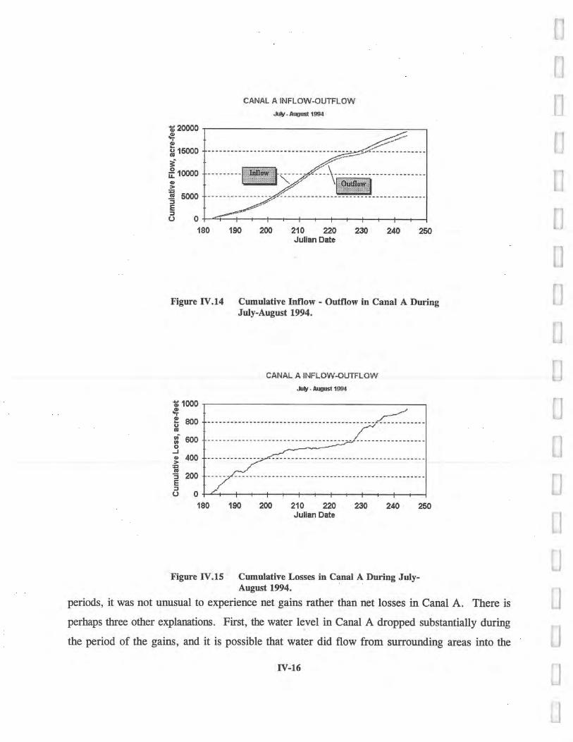
CANAL A INFLOW-OUTFLOW O July- August 1994
d 20000 w d
16000
0 LL 10000
5000 E U 0
- - - -- - - -
-
--- --
--------------
~1 IM
-------------
180 190 200 210 220 230 240 260 Julian Date
Figure IV. 14 Cumulative Inflow - Outflow in Canal A During July-August 1994.
CANAL A INFLOW-OUTFLOW July - August 1994
d 1000 w
800 M H 600
400
3 200 E U 0
---------------------
180 190 200 210 220 230 240 250 Julian Date
Figure IV.15 Cumulative Losses in Canal A During July-August 1994.
periods, it was not unusual to experience net gains rather than net losses in Canal A. There is
perhaps three other explanations. First, the water level in Canal A dropped substantially during
the period of the gains, and it is possible that water did flow from surrounding areas into the
IV-16

canal. The water table is often above the bottom of the canal bottom. Secondly, there has been
some discussion locally about the transition submergence in the Canal B Parshall Flume. There
appears to be some evidence that a value of 70% is more realistic than the published 75%. If
this turns out to be true, then it is possible that some of the gains periodically computed in Canal
A may be due to under estimation of flows in Canal B. Third, and equally likely, is the
observation that the losses are well within the accuracy of the flumes and weirs. Differential
mossing or other growths on one structure or another could shift the measurements enough to
produce similar results. During an earlier attempt to calibrate the Canal B gates, the
watermaster cleaned the sides and bottom of the Parshall Flume with a garden hoe and reported
that the flume reading dropped about 4-5 %.
Although one might argue the absolute magnitude of the water savings associated with
the automation of Canal A, it is difficult to discount the conclusion that the automation produced
savings. Even if the savings were as little as 3% per year, the economic value of the project
would still exceed the cost of automation by twice each year.
IV.3 GENERAL OBSERVATIONS
The estimates of water conservation presented above along with the reports from the
watermaster about travel savings and increased response are significant incentives for other canal
companies to consider canal automation. This is, in fact, happening in Utah. There are,
however, several other observations the authors have made during the two years of this study
that need to be mentioned.
The first observation is that equipment maintenance and calibration are problems the
irrigation companies or districts will have to master if canal automation is to achieve its full
potential. Some would perhaps argue that it is possible to buy perfectly reliable sensors, RTU's,
etc., but this is probably unrealistic. At DMAD reservoir, more than 1,500 measurements on
water levels were made in July 1994. Of these less than 4% were inaccurate as judged by the
authors. More than 80% of these errors were associated with the depth sensor on the reservoir
itself. This sensor is a $750 submersible pressure transducer. Only 20% of the errors found
were associated with either the $300 USU-built water level sensors at the Canal A flume or the
RTU/telemetry system. Any canal automation project must anticipate problems with sensors and
IV-17
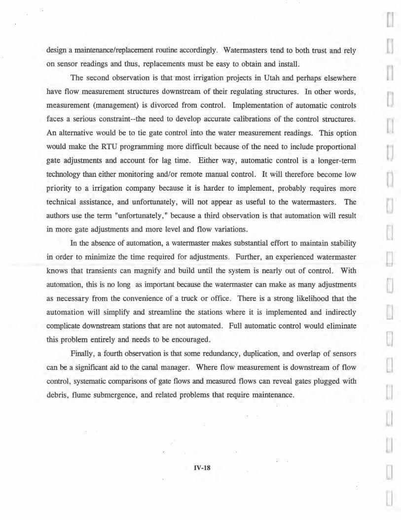
design a maintenance/replacement routine accordingly. Watermasters tend to both trust and rely
on sensor readings and thus, replacements must be easy to obtain and install.
The second observation is that - most irrigation projects in Utah and perhaps elsewhere
have flow measurement structures downstream of their regulating structures. In other words,
measurement (management) is divorced from control. Implementation of automatic controls
faces a serious constraint--the need to develop accurate calibrations of the control structures.
An alternative would be to tie gate control into the water measurement readings. This option
would make the RTU programming more difficult because of the need to include proportional
gate adjustments and account for lag time. Either way, automatic control is a longer-term
technology than either monitoring and/or remote manual control. It will therefore become low
priority to a irrigation company because it is harder to implement, probably requires more
technical assistance, and unfortunately, will not appear as useful to the watermasters. The
authors use the term "unfortunately," because a third observation is that automation will result
in more gate adjustments and more level and flow variations.
In the absence of automation, a watermaster makes substantial effort to maintain stability
in order to minimize the time required for adjustments. Further, an experienced watermaster
knows that transients can magnify and build until the system is nearly out of control. With
automation, this is no long as important because the watermaster can make as many adjustments
as necessary from the convenience of a truck or office. There is a strong likelihood that the
automation will simplify and streamline the stations where it is implemented and indirectly
complicate downstream stations that are not automated. Full automatic control would eliminate
this problem entirely and needs to be encouraged.
Finally, a fourth observation is that some redundancy, duplication, and overlap of sensors
can be a significant aid to the canal manager. Where flow measurement is downstream of flow
control, systematic comparisons of gate flows and measured flows can reveal gates plugged with
debris, flume submergence, and related problems that require maintenance.
I
0 n
Il C
III
IV-18
SECTION V
SOFTWARE
i'1g'Ul-C V .1 1V111111LUY IJI51H ly LVlQY 111 D'QJC MUL11111 allILWUFC.
Two software packages were developed for the Canal A automation, and a third was used
to evaluate the hydraulic characteristics of the canal. The first was a large program for the base
station pc computer. This software provided an interface for the watermaster to perform several
functions. First, he could monitor water levels and flows at both ends of Canal A and determine
if gate changes were necessary. Second, he could remotely control the gates at DMAD
Reservoir and at the divide to either regulate their position or their discharge. And third, he
could examine conditions over any previous monthly or daily period either graphically or
digitally (he could also print data if desired). The base station software (written in C computer
language) also conducted regular polls of the system as part of its routine monitoring function.
All data retrieved by the base station was archived.
V-1

The second software developed for this project was the instruction set in the remote units
necessary to coordinate sensor inputs and initiate gate controls. All sensor inputs were recorded
in the remote unit by taking the average of 50 sequential measurements at periodic intervals and
storing these data in input data registers. When the RTU received a J in a command string,
these data were then sent back to the base station through the radio link. The RTU software
included routines that checked sensor data for errors and included such errors in its base station
transmission. The software included a quasi Proportional Integral (PI) logic to control the gates
in the system under two modes of operation--remote manual instruction and full automation.
The third software package, briefly described in Appendix I, was used to use long-term
simulation capabilities in determining the variable influences of channel roughness and seepage.
Because this software was developed under another program and has been verified and described
elsewhere, only the results of the analyses will be presented in this section.
V.1 BASE STATION SOFTWARE C
The Canal A automation was designed to function under a supervisory control
framework. This necessitated the development of centralized software from which the operating
personnel could monitor and regulate the canal. The core of the software is the communication
routines which connect the base station to the RTU's at the gate sites. The RTU vendor,
Campbell Scientific, Inc. of Logan, Utah, provided software for the CR10 datalogger used in
this study as the RTU, but the software at the time this investigation began was not configured a
for the daily routine of canal monitoring and management. Technical information found in the
company's product literature was not in sufficient detail to allow USU to write its own code to
communicate, command and interrogate the RTU. Consequently, the company licensed part of
their code to USU and the authors wrote a C version of several key program segments.
Because a significant part of the code supplied by the company was in binary form and
could not be used by USU, the base station code as it exists today is actually only an emulation
of the company code.
V.1.1 General Program Description
The base station software is a DOS program executed by typing and entering (~
DMAD.EXE at the prompt. The opening screen (shown below in Figure V.2) represents the U
V-2 a

first level menu and includes five options, all of which are initiated by pressing either the upper
or lower case letter that is highlighted and/or underlined. The first level menu options are: (1)
q or Q to quit program execution and return to the DOS prompt; (2) c or C to enter a program
and system configuration menu, a second level menu; (3) in or M to execute the monitoring and
control program (Figure V.1); (4) o or O to access display, print, or graphical output of all data
monitored by the base station; and (5) s or S to enter a small spreadsheet where sensor
calibration coefficients can be entered or modified.
The entire software interface is graphic so the programming will only run on pc
computers with color or gray scale VGA monitors. Although it is about 300 kbytes in compiled
form, it runs well within the 640 kbyte limits of a typical 80286 or higher-level IBM-compatible
pc computer. There are no extensive computations, so a math co-processor is not necessary.
Figure V.2 Opening Screen of Base Station Software.
V-3
I
D
It is however advisable to use systems with large hard disks if the polling interval is short. For fl
example, the raw data files created in a month using a 30 minute polling cycle will exceed 1
Mbyte. n The Biological and Irrigation Engineering Department of Utah State University does not
warrant the base station software for any specific purpose and does not assume any liability
resulting from use of the software. The programming includes commonly reported procedures
and algorithms for interrogating, managing and controlling the Canal A automation. It can be
modified for other systems, and in fact this is already underway. However, application of the
software to specific situations may involve parameter combinations which violate assumptions
or may require interpretations beyond points of various algorithms resulting in incorrect or
inaccurate results that cannot be anticipated by the developers. Therefore, any use of the
software beyond the application in Canal A unless fully supported by USU is at the risk of the
user.
V.1.2 Program and System Configuration
Before the program can be run, several configuration options have to be set. Shown in
Figure V.3 is a simple spreadsheet where each of the parameters controlling program execution
or access to the field system is identified. The cursor bar can be moved up or down the right
side of the screen to highlight specific parameters which are then entered or changed by simply
typing in new values and pressing the enter key.
The first two lines define the polling procedures. If the user wants the program to poll
the entire system when the program is first executed, a value of .1 is entered. From that point
on, an automatic system poll will occur at an interval defined by the second line value. Polling
requires about 30 seconds per station.
The third input is the number of the RS232 port that is connected to the telemetry system
at the base computer. Generally, this will be a 1 or a 2 representing COM1 or COM2. The
programming automatically opens and configures the port specified. 0 The software has been written to accommodate up to 9 field stations. The internal code
can actually handle up to 255 individual stations. The base station software was designed for
9 stations to allow the Canal A system some room for expansion if the two irrigation companies
V-4

Figure V.3 Configuration Screen for Software and System Setup.
want to monitor and control more of the canals downstream or the reservoir upstream. The
actual number of stations linked to the system is specified by the fourth parameter in the
configuration menu. If there are "n" stations specified, then the first "n" station addresses will
be monitored during each automatic poll.
The next 11 inputs are station addresses for the repeaters and field sites. The two
repeater addresses are for information purposes only. As an example, suppose station 1 was
configured in the field to respond whenever the base called address 617, and further suppose that
the base could not directly contact station 1 because of line of sight or distance problems. Then
it would be necessary to route calls to station 1 through repeaters or other field stations acting
as field stations. This is automatically accomplished by specifying a station address for station
1 as follows: 7.2.617, where the 7 could be a repeater address, and 2 could be another field
station address. The transmissions would go from the base to the repeater then to the other
station and then to station 1 and return. In the Canal A system, the station at DMAD reservoir
V-5

cannot be contacted reliably from the base station and a repeater is used. The watermaster has
a portable base in his truck which is often out of range of the DMAD station. In this case, he
polls the reservoir from his truck through the office base station to the repeater and then to the
reservoir. This feature is a powerful and convenient one for either large systems or those in
mountainous terrain.
The next input is a project suffix code that can be used to flag certain data files. The
code is appended to the end of each file name prefix. For example, the raw data files produced
from the monitoring are all labeled "DATOUT.". When the project suffix is 1, this name
becomes "DATOUT1" and, depending on the month in which the data are collected, will have
a three letter designation appended as the file suffix. In August the raw data file is labeled
"DATOUT L AUG. "
When a headquarters base and a portable field base are operating simultaneously. One
or the other should be disengaged from the gate control algorithms. The next parameter does
this. By specifying a 0, all of the access to flag, gate, and discharge controls are by-passed.
A value of 1 similarly accesses these routines. +L.1
The monitoring map shown in Figure V.1 tends to be a distraction to the watermaster in
the field. Its display can be omitted by specifying "0" on the next line.
Finally, the actual telemetry linkage may take various forms. Three options are
provided. The first, selected by entering a 0 on the last line, connects the computer to a base
radio/modem which then polls the field sites by VHF or UHF signals. The remote sites receive
the radio signal with the same radio/modem system that the base uses to send the signal, and the
remote modem connects the RTU to the system.
A second option is activated when a value of 1 links the base computer to the field
through a telephone connection. At the base station the computer connects to a modem through
which it can communicate over normal telephone or cellular channels. At or near one of the
field sites, a telephone is connected to modem/radio combination which allows an instruction
received at the remote telephone to be broadcast via radio to other remote sites. This is an
interesting connection because it allows access to the system from virtually anywhere in the
world and allows technical support and problem diagnosis to be provided without the expense
and delay of on-site visits.
V-6

The third link is defined by specifying a 2 on the last line of the configuration menu.
This option is similar to the second in that communications with the field sites are accomplished
from the base computer through the telephone system. The difference is that at the remote sites
the telephone and modem connect directly into the RTU rather than to a radio for area-wide
broadcast. Some stations will be located near a phone line and can be tied directly to the
computer. The expanding service of cellular systems makes this an attractive option, particularly
where line-of-sight problems exist and multiple repeaters would be necessary for radio
communication.
V.1.3 Monitoring and Control
When in or M is pressed from the main menu, the monitoring map shown in Figure V. 1
will appear on the screen (unless deactivated in configuration menu, in which case the screen
will be blank). The map includes a list on the lower right-hand side of four display options
activated by pressing the F1, F2, F3, or R (r) keys. The F-keys bring up an RTU data display
as shown in the center of the map in Figure VA for the Canal B station. The F-keys are also
drawn on the map to indicate where they provide monitoring information. Pressing a r or R
erases the data display.
The small second level "Monitoring System Control Prompts" menu in the lower left-
hand side of the screen is displayed by pressing F10 and erased by pressing a or E. It includes
eight options: (1) quit and return to the first level menu, (2) initiate the output programming
which will be described in a later section, (3) erasure of the menu, (4) manual station poll, (5)
flag set/release, (6) discharge targets, (7) gate targets, and (8) time of the the next automatic
system-wide poll. The use of these options will be outlined below.
V.1.3.1 RTU Data Displays.
Management and control of the Canal A system begin and end with the RTU data
display. In the Canal A system, the data displays show the most recent telemetry results for
water levels, gate positions, gate and flow targets, flag status, and RTU errors. When the
display is first shown, all the data come from the raw data file, but during a manual or automatic
poll, the data are those just received from the RTU. During the course of a poll, the base
station requests RTU data more than once, and these data will update as new information
appears, targets are changed, or flags are set/released.
V-7
I

M
P:
A: ar,, UAU ♦.~ 111G 1V1V1111V1 Ul.1 GG11 Q1 111G "dlau ll1QWVLL•
1
Because all of the RTU data display screens are similar, it is perhaps only necessary to
describe the Canal B screen shown in Figure VA But first a note of explanation. The ~l
irrigation system at Delta, Utah is comprised of four irrigation companies which are unique in
many respects. Nearly every canal or lateral bifurcation and all farmer turnouts are metered.
However, the flow measuring structures are generally different than the flow regulating ;
structures. Below DMAD Reservoir, for example, a large rectangular flume about 200 yards
downstream of the reservoir gates measures flow. Below the Canal B gates a truncated Parshall
Flume is used, and below Canal C gates the companies have installed a broad crested weir.2
In other words, their control is segregated from their monitoring. Over the last several years
the companies have been attempting to calibrate their regulator gates with their flow measuring
VA This weir was first developed by John Repogle at the USDA laboratory in Phoenix, Arizona. USU has often referred to it as the Repogle Broadcrested Weir. Reclamation seems to use the term "ramp . flume" more often. In the Canal A project, it is simply called the Canal C Weir. . 0
V-8
0
4

structures to give themselves better flow management capabilities. The automation of Canal A
requires accurate gate calibrations in order to implement gate and flow control algorithms, and
since these calibrations were generally inadequate at the beginning of this study, the RTU data
display contains both the readings from the measuring structures and the gates.
The RTU data display shows five kinds of information. The first is a listing of all sensor
readings at the station. These are labeled in some form as gate openings and gate heads. From
these data the second kind of information, discharges through measuring structures and gates,
are computed. The base station software makes these computations from sensor readings.
although the RTU also makes the same computations. This gives the system some redundancy
and error checking on sensor calibrations. A total gate discharge is listed and can be compared
to the measuring structure reading to check for a number of problems like sensor errors,
submergence, gate plugging, tampering and vandalism, accuracy of the gate calibrations, etc.
Listed alongside the measured gate openings and computed gate flows. are the opening
and flow targets if they have been defined and entered by the watermaster. It is important to
note that for management purposes these data are defined at the base computer, sent to and
recorded in the RTU, and relayed back to the RTU data display from either automatic or manual
polling. This is the third type of information in the display. Neither gate nor flow targets are
acted upon by the RTU unless a flag has been set through instruction from the base station.
Thus, the fourth type of information is the flag status shown near the bottom of the display. A
flag value of 0 means the flag is off, and a value of 1 means the flag in on. These values are
again displayed on the basis of what the RTU has recorded and responded with rather than what
is set in the base station. Any remote manual or automatic adjustment in the system is therefor
a two step process: (1) the watermaster enters, sends, and confirms gate or flow targets; and (2)
sets, sends, and confirms flag values. When the RTU programming detects a flag that is set
(value =1), it loops to its control algorithms which will be described later.'
The final information in the RTU data display is the error status of the system. Any
value other than 0 indicates that the RTU has detected a problem and deactivated all control
V.2 This two-step procedure for initiating remote or automatic controls was designed to make this is very deliberate step for the watermaster and one that has to be sequenced properly for any action to occur.
1a:
r 1

0 logic. When an error is recorded in the RTU data registers, gate and flow targets as well as
control flags can be set or cleared from the base station, but the RTU will take no action. As
will be described below, these errors range from problems associated with gate movement to
sensor readings.
V.1.3.2 Monitoring_ System Control Prompts
The second level menu listed under the "Monitoring System Control Prompts" window
accesses output and controls. As noted, output is discussed under a separate section.
The most basic of the base station
monitoringfunctions is the periodic polling P P g Erase F10 - Menu of the field system. The watermaster can Wed
Next Automatic Poll Im 56 min. determine the time until the next automatic
poll by pressing t or T at the second level
menu. The Monitoring and System Control Prompts menu will be replaced by the small box
shown at the right. When the information is noted, the watermaster returns to the second level
menu by pressing F10.
The base station software uses the Setting Flag Options - Station 2
RTU flag registers to control the logic of the Press AnU Keg To Return
RTU. Pressing f or F at the monitoring I Automatic 2 Manual Remote
menu will create a new window at that 3 Susten-
position as shown at the right. Flag 1 is set
to activate automatic flow control at the RTU site and remains set until either an error occurs
at the site or the watermaster clears the flag from the base station. The second flag activates
a remote manual gate operation in which the RTU moves the gates to their target values, stops,
and resets the flag 2 value to 0. Thus, remote manual operation is a one-time process at the
RTU site while automatic control is continuous. The third flag accomplishes two things. First,
it clears all RTU error values so that automatic or remote manual control can proceed and
secondly, it sets all gate and flow targets to values equal to existing field readings. After a flag
3 is set, any gate or flow adjustments have to be proceeded by re-entering targets from the base
and setting flag 1 or 2.
V-10 ~~j;

a.
I
11
There are several occasions when the
watermaster needs to poll a station manually.
There may be an interest in checking on the
status of flows, water levels, or gate
positions. This is typically the case when in
the field performing other duties. In that case, the manual poll is executed by pressing a p or
P so another small window appears. Then pressing a F-key will route the base programming
through a polling sequence for the station selected. A manual poll will add data to the raw data
file. Note that a manual poll from the portable base will interfere with an automatic poll from
.1 the office base if they are not coordinated.
Figure V.5 Gate Opening Target Screen.
R The last action that can be taken form the monitoring menu is to set gate or flow targets.
Although this step can be taken anytime, it is discussed last because it is the most critical
management step for the watermaster. When either a d (D) or a g (G) is pressed, the
spreadsheet shown in Figure V.5 replaces the monitoring map and display.
V-11
--J

All of the gates in the system that can be targeted are listed with their current settings
tabulated in the first column and their current targets in the second. By pressing a F1, all targets
can be set to 0 in order to completely shut a station off. Pressing the F2, equates all targets
with present conditions (the same as setting flag 3 in the RTU). It is standard practice to press
F2 each and every time this part of the control system is entered. Then, specific values can be
modified to accomplish the regulation or management needed. During the next automatic or
manual poll, all set points are sent to and verified in the RTU's. When the watermaster is
finished, pressing q or Q returns the user to the monitoring map and displays. It is again noted
that no action will be taken in the field unless there are no errors detected and flags 1 or 2 are
off. But it is important to note that it is possible to proceed through these steps with the wrong
targets and cause considerable trouble in the field.
V.1.4 Output
When an o or O is pressed from either
the main menu or the monitoring screen
menu, the screen is cleared and the small
window at the right appears in the lower left-
hand side. This is the output menu which
accesses display, print, and graphic routines. Pressing 1 or L reveals a small window listing all
of the stations being monitored and a file number associated with each. Pressing f or F then
allows the user to enter a file number corresponding to the data file to be output. The user can
also press in or M to define a month for which output is desired, although both month and file
identifications can be entered later as well. All data accessed by the output routines are stored
in the raw data files DATOUT. Depending on the frequency of the automatic polling, these files
may be relatively large. Consequently, the programming also allows the user to consolidate the
raw data files into files containing hourly averaged data. Generally, however, there is little need
to do this since the computers in use today can read and output large data files rapidly.
HI
v
C
10
The important keys in this level of the
output system are d (D), p (P), or g (G)
corresponding to display, print, or graphic
output. When these are pressed another D V-12
0
u

output window menu is displayed as shown here. On the left of the window the user can press
q (Q) to return to the previous menu, or an a, b, or c to change between print, plot (graphic),
or display output. On the right side of the window the choices between flow readings, depth
readings, or gate openings can be made. When the user has configured the output file and
format as desired, pressing the g (G) key clears the screen and displays a standard x-y axis as
shown in Figure V.6 below.
Figure V.6 is the result of pressing o, g, g in the output sequences. Without specifying
a file or a month, the first file and the current monthly are selected by default. Individual data
points are plotted using a small + symbol, and for the case above where there are more than
2000 measurements, a broad line appears.
Each graphics display has two menus to modify the display. In the upper right-hand side
of the screen, the individual measurements for the selected file are listed alongside a number.
Pressing any of the numbers will plot the associated data in different colors.
Figure V.6 Graphics Plot of Monthly Inflow to Canal A.
V-13

PC
At the bottom of the screen, there are the following options. Pressing q (Q) clears the B screen and returns to the previous menu. Pressing d (D) changes the plot from a monthly x-axis
to a daily 24-hour x-axis. The up and down arrow keys change the month, and the page up and tj
page down keys change the day. Pressing an f or F allows the user to change data files and plot
other data on the same axes. Pressing a or E erases and redraws the screen using a x-y scale fl
appropriate to the currently selected file and time frame. Figure V.7 shows the same data on
a daily time axis.
n
0
0
R, Figure V.7 Daily Canal Structure Hydrograph for Canal A Inflow.
Data from any station file can also be displayed in numeric form or printed. Figure V.8
shows the listing of data for the DMAD station. In display or print output, all the readings and
calculated flows are tabulated. To avoid having to prepare separate headings for each station,
a general heading is used, and some columns are empty because a particular station may involve
few numbers or measurements.
If one compares the information the watermaster has at his disposal, it is obvious that the ,
plotted data are much more useful than the displayed data. He can see past history and system
V-14

Displaq Intervals Resume Quit Cull QUattro Year 1994 Month 10 Da-.j 20 File JL
DMAD TELEMETRY READINGS 7 / 1.3 Res Flume Data Gate "eads Gate Openings Gate Ele,j Heads Flow 1 2 3 4 1 2 3 4 5 Flow ft 1 2 cfs feet feet c ff.
65.93 2.29 1.76 139.6 0.27 0.54 0.30 13219 65.93 2.29 1.77 139.9 0.27 0.54 0.30 132.9 65,95 2.30 1.78 140.4 0.27 0.55 0.31 134.2 65.96 2.30 1.79 140.4 0.27 0.55 0.31 134.2 65.96 2.30 1.81 140.0 0.27 0.55 0.31 13412 65.97 8.30 1.81 139.8 0.27 0.55 0.31 134.1 65.96 2.23 1.82 137.1 0.27 0.55 0.31 134.1 65.96 2.22 1.80 130.3 0.27 0.55 0.31 134.4 65.90 2.22 1.79 131.2 0.27 0.54 0.30 133.1 65.94 2.22 1.79 131.4 0.27 0.54 0.30 133.8 65.94 2.23 1.70 132.0 0.27 0.55 0.31 134.2 65.08 2.23 1.78 131.6 0.27 0.55 0.31 134.0 65.97 2.23 1.78 131.6 0.27 0.55 0.31 133.8 65.88 2.23 1.78 131.7 0.27 0.54 0.31 133.3 65.86 2.22 1.77 130.9 0.27 0.54 0.31 133.7 65.84 2.22 1.77 131.2 0.27 0.54 0.31 13313 65.96 2.22 1.77 131.6 0.27 0.54 0.31 133.6 65.85 2.22 1.77 131.9 0.27 0.54 0.31 133.6 65.05 2.24 1.76 133.0 0.27 0.54 0.30 133.4 65.84 2.41 1.81 152.3 0.27 0.54 0.52 157.4 65.82 2.42 1.84 153.3 0.27 0.54 0.52 1156.1. 65.70 2.41 1.04 152.3 0.26 0.54 0.51 154.1 65.80 2.45 1.87 156.0 0.27 0.54 0.52 155.3 65.80 2.46 1.89 156.7 0.27 0.54 0.52 155.4 65.03 2.47 1.91 157.6 0.27 0.55 0.52 157.1 65.80 2.46 1.91 156.6 0.27 0.54 0.52 155.7 65.78 2.46 1.92 156.2 0.27 0.54 0.52 155.6 65.80 2.46 1.93 156.7 0.27 0.55 0.52 157.0 65.79 2.46 1.93 156.6 0.27 0.55 0.52 157.3 65.78 2.47 1.94 156.8 0.27 0.55 0.52 157.3 65.80 2.47 1.94 156.5 0.27 0.55 0.52 157.3 65.79 2.46 1.94 156.5 0.27 0.54 0.52 155.9 65.00 2.47 1.95 157.1 0.27 0.55 0.52 157.2 65.77 8.46 1.94 156.1 0.27 0.54 0.52 156.0 65.00 2.46 1.35 156.1 0.27 0.36 0.52 135.5 65.79 2.44 1.95 153.2 0.27 0.36 0.52 136.0 65.72 2.35 1.92 141.5 0.26 0.35 0.51 122.7 65.77 2.35 1.89 143.2 0.27 0.36 0.52 136.2 65.76 2.34 1.88 142.5 0.27 0.36 0.52 136.3
" M
0 is 0 45 15 45 15
2 45 3 15 3 46 4 16 4 45 15 49 Ifi 45
7 is 7 45 15 45
9 45 10 15 10 45 li 15 11 45 12 15 12 46 13 is 13 45 14 15 14 45 15 15 16 it LG is 16 19 16 20 16 23 Is 25 is 45 17 45 16 16

designation for a file suffix. The user can then rename this file outside of the program to
display, plot, or print the data.
A similar option is initiated when a u or U is pressed. The raw data file is reviewed,
bad values are culled, and the remainder are recorded in a ASCII coma delimited file that can
be imported into one of several popular spreadsheet programs (DATOUTq.wbl). This is also
the feature that is used to provide data to the hydraulic simulation models. It was felt that for
outputting graphic plots of the data, it would be easier to use available spreadsheet programs
rather than attempt to print out graphics images from a DOS-based program. All of the graphs
in Section IV were prepared in this manner.
V.2 SOFTWARE FOR THE REMOTE TERMINAL UNITS "
V.2.1 Modes of Operation
The RTU was programmed to function in four operating modes. These modes are
monitor, remote manual gate move control, remote manual flow control, and remote automatic
flow control. The monitor mode is the start-up condition as well as the fault condition whenever
errors are detected. The remote manual gate and flow control and the remote automatic flow
control modes can be implemented only from the base computer. This controller design gives
the canal management people the opportunity to become comfortable with simpler processes
before progressing to the next mode of operation.
The monitor mode allows management to observe present conditions in the canal. In this
mode only observations are permitted. Flow adjustments must be made in the usual manner--the
canal operators must go to the control structures to make changes. As the management make
the usual adjustments, they are able to observe the results and become accustomed to the
equipment and its capabilities.
Remote manual gate control allows the watermaster to observe present conditions,
determine when gate adjustments are needed, send gate position changes over the radio link to
the site controllers, and then initiate the gate movement remotely by sending a control flag from
the base to the RTU. Once the site controllers receive the control flag, it drives the gate to the
position defined by its internal set point and does not make another change until another gate set
point and flag is sent to the controller. The control flag is reset automatically following a gate
V-16 a

move or an error. This mode has helped the watermaster for Canal A become confident with
the controller's ability and reliability to make desired changes.
Remote manual flow control is similar to remote manual gate control at the RTU. The
difference in the overall scheme is that the operator at the base computer first polls the RTU for
the latest measurement data. From this information the watermaster determines if flow
adjustments are necessary. If they are, he defines new flow targets in the base software. When
the base next polls the RTU, it sends new gate positions which achieve the flow targets.
Under both remote manual gate and flow control, the RTU is programmed in such a
manner that will allow gate movement if it determines that there are no problems. If errors are
detected, the RTU is placed back into monitor mode. The error checking routines that have
been implemented thus far are as follows:
Check for sensors giving no signal input
Check for control gates moving when they are required to move
Check for control gates drifting from last set position
0' Check for bad water level sensor readings
0' Check for water levels that are too high or too low
If the RTU detects any of these problems, the logic is taken out of gate control and a
number is stored in an error register which indicates the water level sensor or gate sensor that
is responsible for the problem. On each program cycle, the error registers are looked at. The
implementation of the water level sensor check routine is simple and has proven to be quite
effective. The water level sensor is continually monitored and compared with the last reading.
If the reading has changed more than 15 cm. (0.5 ft.) within a 20 sec. time period, the CR10
assumes that the sensor is not functioning properly and discontinues gate control.
The fmal control option is remote automatic flow control. Under this. logic, the RTU is
given flow set points rather than gate positions and another control flag is set. The RTU then
checks water levels and gate positions during each program cycle, calculates the flow through
the gates, evaluates whether or not these flows are outside the dead band tolerance, and if so,
computes a revised gate position and moves the gates accordingly. The automatic control flag
remains on until reset from the base or an error occurs.
A variant of remote automatic flow control that was developed (but not tested) toward
V-17

the end of the project was to program the base software to automatically initiate remote manual
flow control during each poll. Thus, instead of the RTU evaluating flow conditions during each
cycle and having the capability for nearly continuous flow control, the base software does so
during each poll. If the polling interval is relatively short, the flow control is nearly continuous.
The advantage of this variation on the concept of automatic flow control is that it simplifies RTU
programming. The disadvantage is that it depends on continuous communication between RTU
and base to be effective. Some monitoring and control systems are being planned that interface
the RTU and the base only periodically, particularly when the base is actually in the
watermaster's truck.
V.2.2 RTU Logic
A flow chart of the RTU logic which was developed for the Campbell Scientific CR10
is shown in Figure V.8. The following is an explanation of how the control logic operates in
the CR10. The program begins by reading the sensor inputs and then calculates flow rates
through the control gates using these sensor values. It then checks for problems--the first being
a static gate error. If the CR10 tries to move a gate and for some reason it will not move, the
CR10 stores a number which corresponds to the problem gate in a storage register. Then on
each program cycle the CR10 looks for a value in the register and stops control if a value is
found. The control program will not allow the CR10 to operate the gates until the problem is
checked out. The program then checks for bad sensors. If the water level has changed more
than 15 cm. (0.5 ft.) in the last 20 seconds, or if the sensors are giving zero input values, the
program assumes that the sensors are not functioning properly, and control is taken from the
appropriate CR10 program loop. When the program detects a problem sensor, a value
corresponding to the sensor is placed in the "bad sensor storage register. "
The program then checks for the gates drifting from the last set position. Drifting can
be indicative of bad gate position sensors, vandalism, or unauthorized gate movement. Once
again, if this problem is detected, a value is posted in the gate drift storage register, and the
CR10 loses control until the problem is dealt with. Finally the water levels are checked to see
if the level is high or low, and if a water level problem is detected, automatic control is
discontinued.
V-18

start
Does Yes No
Manual Gate ate Pos. Differ Read
Analog Inputs Move On Desired Pos.
Shut Off Auto. Compute Flow No Yes or Gate Move through
Will Control Canal Gates
Reset Gate Gate be
Pos. to Max Yes
Driven Beyond
Is or Min. Pos. ax. of Mi
Pos. Yes Static Error
Flag On No
Turn on
No Gate Motor
Check Yes
For Bad Read
Sensors Analog Inputs
No
Have Yes Is Gate Moving
Yes Gates Drifted
From Last
Position
No
No Turn on
Static Flag
Water Levels High or Low No
Does
Gate Pos. Yes Turn Off No Yes
Differ From Gate Motor
Desired
Pos.
Figure V.9 Flow Chart of RTU Programming.
V-19
After is the CR10 if error checking accomplished, checks to see the remote automatic
flow control flag is on or off. If the flag is on, the control program computes target gate
from flow positions the target rates as well as a deadband which prevents gate hunting. These
target gate positions are compared to the present gate positions. If the present positions differ n
from the target positions, the gate control subroutines are called, and the gates are moved. On u
the other hand, if the present gate positions correspond to the target gate positions, the program
initiates the cycle all over again. under operational conditions. This process was repeated with
good results as faults were
The auto/manual gate move routine functions in the flowing manner. This routine causes u
the CR10 to drive the gates to a desired position. In the auto/manual gate control routines the
CR10 compares the target gate positions to the present gate positions and initiates gate movement 1~
subroutines as required. The gate move subroutine operates in the following manner. First, the
routine makes sure the gate will not be driven past the minimum or maximum positions. If the
desired position is beyond the maximum or minimum, the gate is reset to these positions. Once
the positions are checked, the gate motor is turned on and the sensor inputs are read. The lJ
routine then checks to see if the gate is moving. If the gate does not move, the motor is shut
off and a number corresponding to the unresponsive gate is stored in the "static gate error
register. " If the gate is moving, the gate position is compared to the desired position and the
subroutine repeats the entire procedure until the gate is moved to the desired position.
V.2.3 Testing ! 1 lJ
The RTU software underwent nearly two years of testing and development. This
involved two parts, laboratory and field. As will be noted in more detail in the next section,
a prototype gate assembly was built which used the same components as the field system. A
base station was set up to link the base software to the RTU, and a long series of tests were
conducted to evaluate various gate control and error checking routines. When the software
appeared to be working satisfactorily, it was downloaded into the field RTU's and evaluated
identified in the field that had not been detected in the lab. Some problems were detected in the
and corrected lab before field implementation.
One of the problems with the CR10 programming was that it must be connected to the
sensors and gates it is intended to operate before the software could be checked. Unlike a
V-20 a fl

a more conventional language, the RTU software was only operable in either the prototype gate
or field situations. Since the field installations were more complicated than the prototype gate
some programming errors in the field RTU's were unavoidable.
As expected, the monitoring capabilities of the RTU were its strong point since it was
originally designed as a datalogger. Remote manual gate and remote manual flow control are
relatively simple procedures for the RTU and were tested by the watermaster during the 1994
season. DMAD Reservoir was operated in July and August with minimal site visits. The
remote automatic flow control was field tested during brief periods when the authors were
visiting the field site. The watermaster was reluctant to use this mode of operation for extended
periods.
While the CR10 met and exceeded USU's expectations, there was one problem that
repeatedly occurred and should be mentioned. During the programming cycles when the gates
were being moved and monitored, the programming was looping through subroutines. The base
software had the option of monitoring the field RTU's continually during gate movements and
was sending a "K" command every 5-8 seconds asking for a data dump from the input resisters.
In the first versions of the programming, the CR10 had difficulty responding to base station polls
during gate movements. The RTU program was modified to pause program cycling for about
0.1 second each cycle, and the problem became sporadic. During the problem, the RTU
functioned reliably and normally at the field site, but the base received data with transmission
errors.
The problem was reported to Campbell Scientific and future arrangements will be made
to identify and remedy the problem. Nevertheless, the problem was very disconcerting to both
USU and the watermaster. The first time it was noticed, the watermaster made a high-speed
emergency trip to DMAD Reservoir thinking the system had gone out of control, only to find
that all the gates were set precisely as he had instructed the RTU. It was later discovered that
the data transmission problems during gate adjustments only appeared during continuous polling. e
A manual poll a short time after the gate move flag had been sent, resulted in normal data
transmission and verification that the gate had been moved.
In summary, the RTU programming was developed, verified, and tested under field
conditions and has proven reliable and effective. However, as yet the remote automatic flow
V-21

control has not been judged safe or reliable by the watermaster for extensive. There may be
intermediate steps which can be taken in future implementations to facilitate the transition
between the monitoring, remote manual control, and remote automatic control.
V.3 SIMULATION SOFTWARE
Perhaps one of the most important uses of canal simulation is provide insights into the
complexity of the distribution system and hydraulic behavior, the lack of field (or errors in) data
for canal operation, and channel carrying capacity restrictions. The constraints and uncertainties
imposed by system complexities, for instance, can be partially removed through use of the
simulation model because it provides a view of alternative operations in a potentially large and
branching network of supply canals. Without this kind of model, and in the absence of
automation hardware, canal system operation is limited to simple hand calculations and
operational experience. This, in turn, may restrict operation to a narrow range of water
distribution conditions, even though there may be many years of practical experience.
The specific uses of a canal simulation program are outlined in several technical
publications, and this report does not attempt to reiterate them. In the early stages of the Canal
A automation project there were two questions that were addressed by simulation: (1) how the
growth of bank vegetation and mossing affected capacity; and (2) how much of the recorded
losses were the actually result of seepage.
V.3.1 Software Configuration
The writers utilized data from Section 3 the CanalMan software to simulate upstream and
downstream depths in Canal A over the period of July 15 - August 14, 1994. The input data
included the inflow hydrograph from the telemetry readings at the Canal A flume, the outflow
hydrographs from the flume in Canal B, the weir in Canal C, the computed gate hydrographs
from the West Ditch and the hydrographs from the Pump Ditch, as well as an average of the
three measured channel cross-sections, and the average slope of the channel,. The data were
from the automatic polling during the period of July 15th through August 14, 1994. No
information was use to describe the variations in the Canal A channel slope, the channel cross-
sections (which were known to be substantial), nor information on the conditions prior to July
V-22
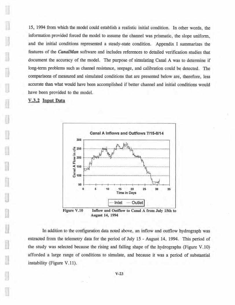
15, 1994 from which the model could establish a realistic initial condition. In other words, the
information provided forced the model to assume the channel was prismatic, the slope uniform,
and the initial conditions represented a steady-state condition. Appendix I summarizes the
features of the CanalMan software and includes references to detailed verification studies that
document the accuracy of the model. The purpose of simulating Canal A was to determine if
long-term problems such as channel resistance, seepage, and calibration could be detected. The
comparisons of measured and simulated conditions that are presented below are, therefore, less
accurate than what would have been accomplished if better channel and initial conditions would
have been provided to the model.
V.3.2 Input Data
Canal A Inflows and Outflows 7115-8114
300
250 -------------•---,--- ..-...r -...k-'.----Y -' ..............................................
C ,N
200 '
------- ---------- ------------------------------- O ~ h
Q150 . .......................... ............. ................... ----------- ----------------
UU 100 ..................................•-•-•------------•---•------..........-------- ......................
50 L
0 5 10 15 20 25 30 35 Time in Days
Inlet ----- Outlet
Figure V.10 Inflow and Outflow to Canal A from July 15th to August 14, 1994
In addition to the configuration data noted above, an inflow and outflow hydrograph was
extracted from the telemetry data for the period of July 15 - August 14, 1994. This period of
the study was selected because the rising and falling shape of the hydrographs (Figure V.10)
afforded a large range of conditions to simulate, and because it was a period of substantial
instability (Figure V.11).
V-23

Canal A Inflow - Outflow 7115 - 8114 40 -
30 ------ --------------------------------------------------------------------------------------------------------
2D------ -- - -------- -------------- — -------- -------- .................................
~ 1D e
3 Q ! V
~
.
-10 ---------------------- -- `----- --------- ----------
-20 -- " ...........................
-30
D 2 4 B 8 10 12 14 16 18 20 22 24 26 28 30 32 Time in Days
Figure V. 11 Canal A Inflow Minus Outflow During the Period of July 15th through August 14, 1994.
V.3.3 Evaluation of Channel Resistance
Figures V.12 and V.13 compare the measured upstream and downstream depths in Canal
A with simulations using two values of the Manning n which were used to quantify resistance.
The simulated water levels were generated with Manning n values of 0.009, the best fit value,
and 0.0045. These values were somewhat less than published values for earthen canals, but the
velocity in Canal A was quite slow.
Figures. V.12 and V.13 show that the effects of varying roughness in this range over the
31-day simulation period. Changes in upstream water levels are significant, but downstream
effects appear substantial only during periods of large water level fluctuations. It is not certain
how much effect on channel resistance is caused by the growth of bank vegetation and moss, but
one would expect that it might easily result in a change of this magnitude. Conversely, a channel
cleaning might create the same effect. However, much larger fluctuations are caused by the
operation of the downstream gates and the imbalances in the inflows and outflows. As a result,
it is concluded that for Canal A, the effects of bank vegetation and mossing probably do not
impact operations. This conclusion is somewhat verified by the irrigation companies because
their Canal A maintenance schedule over many years has been sporadic.
V-24

Measured 1 Simulated Upstream Depths At Various Manning n Values
3.5
W 3 W LL c 2.5
> 2 W J
.r 1.5
c~ 1
0.5
0 5 10 15 20 25 30 35 Time in Days
Figure V.12 Comparison of Measured and Simulated Upstream Depths in Cana A as a Function of Channel Resistance.
Measured I Simulated Downstream Depths At Various Manning n Values
B
d 5.5 LL c 5
m
4.5 `m
4
3.5
Qi44+15
h, f i'• ! j
0 049
t ^`
- - - - - - - - - - - - - - - - t - ------------ ' - - - - - - - - - - - - - - - - - - - - - - - - - - - - - lYleaswred..
0 5 10 15 20 25 30 35 Time in Days
Figure V.13 Comparison of Measured and Simulated Downstream Depths in Canal A under Various Manning n Values.
V-25

V.3.4 Evaluation of Channel Seepage
Following the same procedures, the values of seepage rate were varied from 1.46 cfs
to 2.57 cfs (the best fit) to determine if a particular value could be determined from a "best-fit"
of the upstream and downstream depths. Figures V.14 and V.15 compare the measured and
simulated depths as a function of seepage rate.
Measured / Simulated Upstream Depths At Various Seepage Loss Rates in CFS
4.5
w 4 ---------------------- --------------------_------ m
.:.-- 3 --- .,,
> 2.5 -------- • . ........................ - ........... ............. .
2 ------------------------------ ~
m 01.5 - .................................. -•----------------......------............... ..
1 - - - - - - - 0.5
0 5 10 15 20 25 30 35 Time in Days
Fig. V.14 Comparison of Measured and Simulated Upstream Depths in Canal A Under Different Seepage Rates.
Measured / Simulated Downstream Depths At Various Seepage Loss Rates in CFS
s
m LL 56 6 m a J5 L m
4
3
x .......... - ----------------- ----- -------- --
------------------ •1 N.: y.. .~.......... . . Mepsuroi: r=
0 5 10 15 20 25 30 35 Time in Days
Fig. V.15 Comparison of Measured and Simulated Downstream Depths in Canal A Under Different Seepage Rates.
V-26

It is apparent that seepage rates must be accurately estimated in order for a simulation
model to closely simulate water levels at either end of the canal. In Canal A, a three foot error
in computed downstream water levels results from an error in seepage rates of only 1 cfs. The
corollary of this conclusion is that if one assumes that models have been proven, then fitting
seepage rates to a model is an effective method of determining seepage rates in the field. There
is some verification for this observation in the field data. For example, the average difference
in Canal A inflows and outflows shown previously in Fig. V.11 is 2.52 cfs.
Another important observation gained from the simulations was that seepage rates have
to vary to account for additions to and from bank storage. For instance, from about day 11 until
day 20 of the simulation ( July 26 - August 5), the water levels in Canal A dropped about one
foot. During this period, the seepage rates have to be negative (inflow to the canal) in order for
the simulation to proceed. Thus, the average seepage rate of 2.57 cfs over the simulation period
is somewhat misleading since the fluctuations range from about 7 cfs of loss (the average value
of the July 1st - August 31st period) to about five cfs of gain. Figure V. 16 shows the estimated
variance of seepage rates during the simulation period.
Seepage Losses in Canal A 7115 - 8114
a
w6 -------------- ------------------------------------- ---------------------------------------------------------- v
4 -------------- m 0
2 ......................................................................................... ...................... w fA
J 0 CD m 0.-2 ............................................................. ................................................ CD CD
(0 -4 ----------- ---------------------- ------------ --------- ----------------- -------- --------------------
_g
0 5 10 15 20 25 30 35 Time in Days
Figure V.16 Estimated seepage loss rates in Canal A during the simulation period.
V-27

'Il
There are a number of interesting recommendations that emerge from the simulation of
Canal A. The evaluation of seepage rates will be of particular interest to the watermaster
operating Canal A. If he relies primarily on remote manual control and monitoring to manage
the canal, he will be continually adjusting the downstream gates for fluctuations in water level
caused by the imbalance between the releases from DMAD Reservoir and the downstream
diversions. He can reduce the transients in the canal substantially by adjusting DMAD releases
to the downstream demand plus seepage losses (or gain).
Based on the simulation of Canal A in 1994, the writers would recommend that DMAD n
release exceed downstream demands by seven cfs during period of steady demand of 200 cfs or u
more. When additional water is diverted from Canal A to satisfy a new downstream demand
and adjustments at DMAD Reservoir have yet to stabilize the canal at a new level, the releases
can be adjusted for a net gain of about five cfs in the canal flow as bank storage returns to the (~
channel. In late July and August the canal water levels will decrease because the total demand ~}
decreases and the losses will average about 2.5 cfs.
There are undoubtedly a number of evaluations yet to be made in Canal A and in other
canal systems using the simulation models now available. Such evaluations are beyond the
expertise of most watermasters and company or district personnel, but could be provided by state
and federal extension specialists, research institutions, and consulting firms.
11
0

SECTION VI
TECHNOLOGY TRANSFER
The transfer of the technology of canal automation during this investigation involved
three phases: (1) demonstration and explanation of canal automation to state and local irrigation
interests in Utah, (2) local training of the Canal A watermaster, and (3) publication of the results
for irrigators outside Utah.
VIA ADVERTISING CANAL AUTOMATION
The personnel responsible for the majority of irrigation projects, both large and small,
are aware of canal automation and have at least seen gates that automatically regulate upstream
water level or downstream flow. The irrigators they serve are knowledgeable about automatic
methods of applying water to their fields. In fact, there is a lot of automation technologies in
use by the general public every day. What they generally have not seen or become aware of is
that variations on this technology can be applied to the management and operation of irrigation
systems to conserve water and increase scheduling flexibility.
VI.1.1 Preparing Visual Aids for Demonstrations
Three visual aids were developed to communicate with irrigators and project personnel.
The first was the project map shown as Figure IV. 1. The map was drawn and recorded as a
graphics file on the base station pc disk. The base station software displays this map as noted
in the previous section. The purpose of the map display was to "catch the eye" of irrigators
during presentations of the Canal A project. Data displayed on the screen was therefore given
a physical dimension for those who are not familiar with the canal layout.
The second aid was a large 4 foot by 6 foot wall display of the Canal A system built as
a senior design project in the Department of Electrical Engineering at USU. The display is a
map of the Canal A system with LCD displays of the flows from each gate and flume in the
system. The base station software updates the data displayed at the end of each poll. The
VI-1

purpose of this display, besides that of the electrical engineering student,' is to illustrate the real-
time monitoring that is possible. The display shows the present status of the entire canal to the
Boards of Directors of the Delta Canal Company and the Melville Irrigation Company who
participated in and supported this study. Of course, farmers throughout the Central Utah region
often visit the local office and see the display during a discussion of the merits of canal
automation.
The third aid is a full-scale automatic canal gate model which USU calls "Robogate. "
It became apparent that irrigators needed to see the entire concept working to appreciate what
can be done, what is involved, and how it would operate. A photo of Robogate is shown in
Figure VI. 1. The model is equipped with the same RTU, water level sensors, and gate position
sensors used at Canal A. The base station software is the same as that used in Delta, and the
RTU programming is a subset of the Canal C gate monitoring and control code. A special
display map was prepared for the software showing the gate in operation. This map is shown
below as Figure VI.2. The function of the Robogate software is the same as described in the
previous section.
VI.1.2 Presentations and Demonstrations
For USU the mechanism for technology transfer is institutionalized in its state agricultural D extension service. In June of 1993, shortly after the Canal A system had been installed, the
State Irrigation Specialist for the extension service advertised a "field day" throughout Utah.
Nearly 50 irrigation company (or district) personnel, irrigators, and state and federal agency
personnel visited Delta where an explanation of the Canal A system was presented by the authors
and the Canal A watermaster. The presentation involved a demonstration of the base station
software and a field tour of the Canal A RTU sites. The message was simple-- canal automation
can be implemented within a reasonable time frame, at a justifiable cost with significant benefits
to the company or district. Q
VIA This student project won second place in the state-wide competition among student engineers in n Utah. 0
VI-2 (~
0
u

j
~~
I hl
I r~~
0
Figure VIA Photo of Robogate Showing an Full Scale Automatic Canal Gate with Upstream and Downstream Water Level Sensors, Gate Position Sensor and
D Complete RTU.
I
III Figure VI.2 The Robogate Monitoring Display.
VI-3

D
CPS In early March 1994 the authors and personnel from the Utah Projects Office of
Reclamation made a presentation on canal automation at the Utah Water User's Workshop in St.
George, Utah. The USU presentation involved a demonstration using Robogate with the pc
screen projected on a large screen in the room. It was possible to first explain the components
of canal automation and then demonstrate monitoring, remote manual gate control, and remote
automatic flow control.
Throughout the project the concept of canal automation has been demonstrated at USU
using the model gate. Presentations have been made in several locations in Utah as well as part
of USU Extension activities.
VI.2 LOCAL TRAINING
Canal automation is not a standardized technology; nearly every irrigation system has a
unique combination of structures and management. Therefor, the specific control, monitoring,
and mechanization must be tailored for each system. Large irrigation projects can afford to hire
technical staff to maintain various parts of an automatic system, but small and medium projects
must rely primarily upon their operational personnel. Automation that is overly complicated,
difficult to service, replace, or expensive may not be acceptable in the short-term nor sustainable
in the long-term. Thus, a critical element of future projects has to be sufficient training and
technical support to allow watermasters and other field personnel to operate and maintain their
own systems.
When this project began, a key objective was the transfer of the technology to the Delta
Canal and Melville Irrigation Companies, since USU cannot afford a long-term technical
assistance program. The benefits of canal automation would be completely lost throughout Utah
if the Canal A control system were installed and then failed when the canal companies took over
because of maintenance.
From the beginning of installing instrumentation to the final testing of the software, the
investigators worked side-by-side with the Canal A watermaster. Explanations were provided
for each step and careful attention was given to helping him understand the function of each
system component. His suggestions were incorporated into revisions of the software, and USU
V14
0
L
'I]
C1'
0

equipped his truck with a portable base station so he could access the automation at any time of
the day or night from wherever he might be. The watermaster was encouraged to experiment
with the system. On a number of occasions when USU toured other groups through the project,
the watermaster was invited to conduct a field visit and explain the way the system was being
used.
As noted, the watermaster tested and experimented with the system. There were several
times a problem occurred, such as a radio failure, and he resolved it without notifying USU.
A number of his observations became invaluable revisions to the electronic designs and
software.
VI.3 PUBLICATIONS
One of the questions most asked during presentations and discussions is whether or not
something has been written about canal automation. There are, of course, several technical
reports in the engineering literature, but it is difficult to find something suitable for irrigators.
In the June 1994 issue of Utah Science, a publication summarizing all of USU's
Agricultural Experiment Station research, an article entitled, "Canal Automation... " was
published. Utah Science is distributed throughout Utah, all Land Grant Universities in the US,
the US Department of Agriculture, and in Canada. The article presented a first level message
about the advantages of canal automation. (Copies can be obtained through the authors).
A more detailed message was prepared for Utah irrigation projects in the form of a
proposal to the Utah Permanent Community Impact Fund Board that could be submitted by
irrigation companies through their respective county organizations. This document describes the
purpose and goals of canal automation in terms of water conservation and scheduling flexibility,
reviews the results of this investigation, outlines a procedure for an individual company or
district to initiate a demonstration project on canal automation, describes the components of
canal automation, and summarizes the costs. This document was first written as a Extension
Service Fact Sheet for distribution through county agents, but it was later targeted for the
companies interested in funding support for a pilot program.
VI-5


SECTION VII
CONCLUSIONS AND RECOMMENDATIONS
VII.I CONCLUSIONS
1. Canal automation can reduce losses from conveyance and distribution of irrigation
water through canal networks. In this study, the seasonal losses in 1993 and 1993
were reduced more than 50%. The precise and frequent monitoring of water
levels and gate positions substantially improves water measurement and thus
reduces the water that cannot be accounted for and allocated. The ability to
monitor the entire system accurately from a central location aids the canal
operator in making more reliable and timely gate or flow adjustments. When the
canal operator becomes comfortable with the automation, water levels in the
canals can be reduced to lower seepage and thereby eliminate unregulated spills.
2. Canal automation can improve the flexibility and responsiveness of canal systems.
The capability of an operator to make gate and flow changes almost instantly
from an office or mobile base station allows the system to respond substantially
faster than under traditional manual control practices. Canal automation is likely
to be the only feasible means for some irrigation projects to implement on-
demand scheduling.
3. Widespread acceptance of canal automation will occur rapidly. The importance
of accurate flow measurement, lower operating levels, and more timely and
reliable system response to irrigator demands are already understood by canal
managers and farmers. The automation, however, must be adaptive and low -
cost, at least initially. The principal requirement for meeting both conditions is
that the automation be adaptable to existing regulation and outlet structures where
possible. It must also be useable within existing management practices and be
easy to adjust, diagnose, and repair.
4. Personnel within the irrigation community are quite capable of mechanizing
existing gate structures. They will need technical assistance with the design and
installation of sensors, canal-side and base station processing, and control
V11-1

equipment. These people are also quite capable of diagnosing and correcting
problems with the electronic components of automation. They are probably not
capable of software modifications for either the base or canal-side computers.
5. Water level and gate position sensor costs were too high at the beginning of this
investigation, but are now comparable with sensors that can be designed and built
locally. While the need for continued development of low-cost sensor systems
for canal automation still exists, there is probably little justification for local
fabrication.
6. It is unrealistic to conclude that electronic components like sensors, radios,
modems, computers, etc. will be entirely trouble-free. Since technical assistance
for irrigation companies and districts is limited, redundancy in many cases will
be cost-effective, not only to safeguard the canal operation but also to diagnose
and correct problems like flow structure submergence and gate plugging.
7. While there are several manufacturers of devices that can be used as RTU's, only
one, the Campbell Scientific CR10, was tested in this project. It is rugged,
reliable, low cost, and adaptable. The unit is primarily a datalogger, but it also
has a number of features generally associated with industrial controllers that make
it a good canal automation RTU. Early versions had limited memory and gate
control algorithms were limited, but present versions have adequate memory for
standard gate control and error checking algorithms. The CR10 uses a
proprietary programming language that is more difficult to debug outside of the
RTU site because it needs to be connected to sensors and switches to be fully
tested. However, it is a simple and powerful language, that once mastered can
be used effectively. It has some difficulty communicating while executing gate
move routines; the nature of this problem is unknown at this time and may be
a software fault.
8. A very useful feature of the Campbell Scientific RF95 modem is its addressing
which allows any field site to act as both a RTU and a repeater linking the base
to another site. In the mountainous terrain of Utah, line-of-sight radio
transmissions are not feasible for all stations and repeaters have to be used.
VII-2

Recent coverage of cellular phone service will mitigate some of these problems.
9. The one component of the equipment that did not work as well as it should was
the radios. Components supplied by Campbell Scientific, Inc. were not rugged
nor reliable enough for the conditions a canal system operates under. Alternative
radios designed specially for field data telemetry are available and should be used.
10. The key to improving canal management in the age of the microcomputer is
software. Software for both the RTU and the base station proved to be a major
undertaking in this investigation, and most of it can be transferred to use at other
sites without difficulty. However, because irrigation projects are configured and
operated in many ways, some software modification will be required for all new
installations. Nevertheless, the ability to not only note existing conditions but to
review data from the last few days, weeks, and months are important management
inputs to canal operations.
VH.2 RECOMMENDATIONS
1. The technology for mechanizing, automating, and controlling selective
components of irrigation distribution systems should be made available through
a widespread program of technical assistance and cost sharing. The results of this
project have shown that losses in a distribution system can be reduced by this
technology. These losses exceed the losses due to seepage for which extensive
canal lining has are been implemented, and comparable losses can be reduced for
a fraction of the cost of canal lining. Few irrigation companies and districts have
the in-house expertise to initiate canal automation, but projects such as this,
where one or two sites are automated and careful attention is given to technology
transfer, will allow them to expand, adapt and implement automation on a larger
internal scale.
2. Since most existing irrigation projects separate water control from water
management and allocation by installing separate structures for measurement and
regulation, canal automation by adapting controls to existing structures faces the
problem of control structure calibration. It is apparent that little or no
VII-3

consideration for flow measurement was made when many of these structures
were designed and constructed. As a consequence, the hydraulic characteristics
of many are not amenable to standardized equations and procedures. Gate
calibration needs to be an important component of technical assistance provided
to canal automation efforts.
3. Irrigation companies and districts that have historically operated on a rotational
or continuous flow basis can move toward on-demand scheduling, but the
administrative and regulation problems are formidable without remote monitoring
and control. Selective automation of critical structures, particularly those at
remote locations, is a cost-effective means of facilitating a change in scheduling.
A pilot study should be undertaken when a project shows interest in going to on
demand scheduling to determine the associated processes and costs.
In a canal automation project, particularly one involving a private company or
district, the primary benefits will initially derive from monitoring, followed by
remote manual control, and ultimately by automatic flow or water level control.
Monitoring and remote manual control have been demonstrated and proven in this
study, but automatic control was given limited testing and did not reach the stage
of complete local acceptance. The increased transients in a canal that are likely
when remote manual control is implemented affect the management of the system
more than the canal operators and managers perhaps appreciate. Automatic
control should be more fully tested and demonstrated as a means of improving
canal operations further. This takes longer than one or two irrigation seasons and
should therefore be part of a larger, longer-term technical assistance package for
irrigators.
5. The authors are satisfied with the Campbell Scientific CR10 as a canal-side RTU
and recommends the device for that purpose. However, there are several such
devices available that may serve as well and should be evaluated.
The software that operates a canal should be interfaced or merged with the
software that is used for other management functions within an irrigation
company or district. This would reduce the need for having one computer
VIEW

dedicated solely for canal control and monitoring for which the processors are
actually in use a small fraction of the time. Linking a control function to
administrative functions would streamline both canal operation and project
management.
VII-5


APPENDIX I
DESCRIPTION OF THE CANAL SIMULATION MODEL'
A_1 BACKGROUND
The United States Agency for International Development (USAID) funded a project called Water Management Synthesis II during the mid-1980's. Part of this project was designated to support the development and application of computer models for use in improving irrigation water management. Under that part of the project, a transient-flow model called CANAL was developed for simulating canal hydraulics and for calculating control structure and turnout openings according to specified delivery schedules (Merkley 1987). The model was originally written in the Pascal programming language on a Hewlett-Packard workstation. It was later transferred to an IBM-PC/AT microcomputer under the MS-DOS operating system. The current version of the model was entirely rewritten in the C language as an MS Windows application. Included in this revision have been numerous new features and improvements to the technical routines and interface. This new version is called CanalMan.
Beginning in 1979, a similar effort was undertaken within the Bureau of Reclamation, first as a main frame application and later to a pc version (Rogers and Merkley, 1993). This model is named USM (unsteady model) and differs from CanalMan only in terms of select features, solution methodology, and interface.
Both the Pascal version of CanalMan and the USM software were evaluated in 1993 under a cooperative program among several research groups in the Western U.S. The results of this evaluation for the CanalMan software is reported by Merkley and Rogers (1993).
A.2 MODEL DESCRIPTION AND APPLICATION
The CanalMan software was developed for performing hydraulic simulations of unsteady flow in branching canal networks. The model is intended primarily for use in operational and training activities but can also be applied design and analysis. The model can be used to simulate canal operations to generate operating schedules through a centralized control logic as well as several local control options. Several of the common types of local gate automation schemes can be easily selected and calibrated through the model interface.
Results from CanalMan include flow depths in the canal reaches, volumetric flow rates, and control structure (gate) settings -- all as a function of time. Simulation results can be viewed in numerical and graphical formats on-screen, and tabular results can be written to text files. Direct
A.1 This description is taken from the user's manual for the Canakwan program, Version 4.0, April 1994.
A-1

printouts ofthe tabular results can also be obtained from the model. Changes in selected reach depth profiles, downstream target levels and gate settings can be monitored during a simulation through graphical flow profile windows. Reach inflow and outflow rates, modes and statuses can also be viewed during a simulation.
The model is highly interactive and includes integrated data editing capabilities with numerous options for canal system configuration, hydraulic simulations, and output of results. Internal data cross-checking and input range restrictions on individual parameters help prevent infeasible configurations and operating conditions. Canal networks are built interactively by inserting and arranging nodes graphically in a system layout window on-screen. Nodes represent locations of flow control structures and channel bifurcations.
Input data are modified easily for successive simulation studies. Multiple trials can be completed rapidly. Simulations can start, stop, pause or step through an analysis with the ability to change input data at any time and view intermediate results during a simulation.
The model's different modes of operation offer a great deal of flexibility. Structure settings and discharges can be specified through time graphs entered before a simulation. They can be changed at any time during program execution. Structure settings can also be generated through a gate scheduling mode, and local gate automation algorithms can be applied. The program is an excellent tool for duplicating day-to-day operations of real canals.
A.3 TECHNICAL FEATURES
CanalMan implicitly solves an integrated form of the Saint-Venant equations of continuity and motion (Strelkoff 1969) for one-dimensional unsteady open-channel flow. Computational nodes, which are automatically inserted along the length of a canal reach, are used internally by the model. Simulations can be started by filling an empty canal system, continuing a previous simulation, or from a specified steady or unsteady flow condition.
The model will directly simulate the layout of most canal systems, including branching canals. Canal reaches are separated by in-line control structures such as gates, weirs, and pumps. Several in-line structures can be independently simulated in parallel at the downstream end of a canal reach. Turnouts can be used to remove water from the simulated canal system, or divert water into laterals or sub-laterals within the system. Turnout operations can be simulated by specifying a setting (the model calculates flow rate), specifying a "demand" flow rate (the model calculates setting), or giving an "actual" flow rate in which the model simply assumes the flow is correct. Time graphs of flow rate and setting can also be created for individual turnouts and applied to these three operational modes.
A variety of in-line and turnout structures can be selected from the editor for inclusion in a system layout, including weirs, underflow gates, pumps, "non-structure" section changes, and uniform flow boundaries. The inflow rate at the system source can be "manually" specified,
A-2
calculated according to local conditions, or calculated according to system-wide delivery requirements.
A.4 MODEL LIMITATIONS
The model cannot analyze channel de-watering, rapid flow changes (such as bores and surges), negative flow at in-line structures, hydraulic jumps, or supercritical flow. Looping canal systems are not handled. The computational time step can be from one to ten minutes, in whole minutes only, so hydraulic phenomena involving changes on the order of seconds are not adequately handled.
Channel cross-sections can be either circular or trapezoidal. Trapezoidal sections can be non-symmetrical. The cross-sectional shape and size can change from reach to reach, but not within a reach. Thus, the model uses either circular or trapezoidal sections to approximate non-prismatic or natural channel sections.
Maximum system dimensions include forty 40 reaches, with up to 20 turnouts, 4 lateral ofltakes, and 9 in-line structures per reach. Absolute maximum number of structures in an entire canal network are one 100 in-line structures, 200 turnouts, and 12 lateral ofltakes.
The maximum number of system levels is four, meaning that there can be one primary branch and multiple secondary, tertiary and quaternary branches. Reaches at the quaternary system level cannot contain lateral ofltakes. The maximum duration of a simulation is 65,530 time steps, which depending on the size of the time step would be from about 45 days to 455 days. However, if results are output to disk files during a simulation, the disk may become full before this limit is reached.
A.5 REFERENCES
Merkley, G.P. 1987. Users Manual for the Pascal Version of the USU Main System Hydraulic Model. Utah State University, Logan, Utah.
Merkley, G. P. and D.C. Rogers. 1993. Description and Evaluation of Program Canal. J. Irrigation and Drainage Div., ASCE 119(4):714-723.
Rogers, D. C. and G. P. Merkley. 1993. Description and Evaluation of Program USM. J. Irrigation and Drainage Div., ASCE 119(4):693-702.
Strelkofl; T. 1969. One-Dimensional Equations of Open Channel Flow. J. Hydraulics Div., ASCE 95(3):861-876.
A-3

r_j r
r,"
I I I I
I I I I I ll


