

1

2
Reading “Quiz”

3
Review • Often in PL we try to form judgments about
complex human-related phenomena
• The right answer arises from a complex interaction of features
• ML can help us model this sort of thing

4
Examples • Bug Reports
• Readability
• Documentation
• Program Synthesis
• Genetic Programming
5
Last Time • ML Basics
• ML (heart) PL
• K-means Clustering (Unsupervised)
• Linear Regression (Supervised)

6
This Exciting Episode
• Quick review of basics (now with formalisms)
• “Advanced” ML Algorithms (supervised only)
• Coercing a problem in ML
• Evaluation Techniques
• Other “useful” info

7
Review: Supervised Learning
Given a set of example pairs (instances, answers)
Find a function (in the allowed class)
That minimizes some cost function
},),({ YyXxyx
FfYXf ,:
,: FC
8
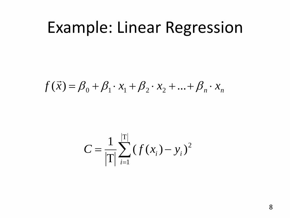
Example: Linear Regression
1
2))((1
i
ii yxfC
nn xxxxf ...)( 22110

9
Example: Logistic Regression
1
2))((1
i
ii yxfC
zexf
1
1)(
nn xxxz ...22110

10
Learning Goals
Numerical (scalar values):
• 3.456, 3.457, 12.3452
Ordinal (categories with an ordering):
• Low, Medium, High
Nominal (categories with no ordering):
• Tree, Car, Fire
11
Advanced ML Algorithms
• Support Vector Machines
• Bayesian
• Decision Trees
• Artificial Neural Networks

12
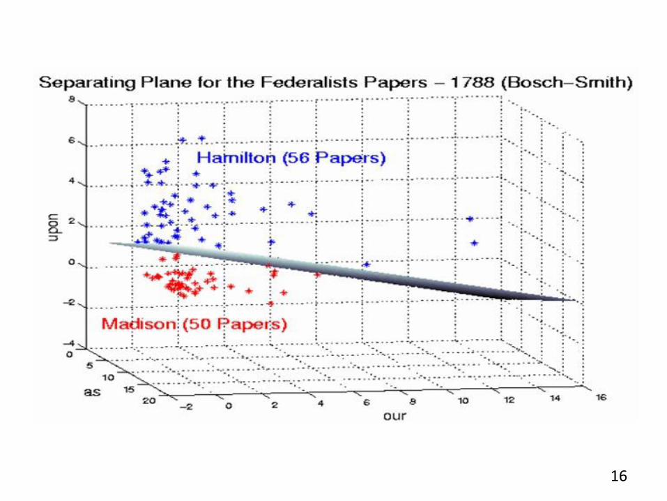
Support Vector Machines

13
Support Vector Machines
Generalized Linear Classifiers
Binary Class Version:
• Given Training Data
• We want to give the hyperplane that divides the points having y=-1 from y=1 that has “maximal margin”
}}1,1{,),({ yxyx p

14

15
16
17
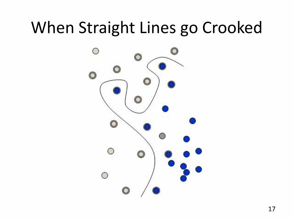
When Straight Lines go Crooked

18
When Straight Lines go Crooked
• Rather than fitting nonlinear curves to the data, SVM handles this by using a kernel function to map the data into a different space where a hyperplane can be used to do the separation.

19
When Perfect Separation is not possible
• SVM models have a cost parameter, C, that controls the trade off between allowing training errors and forcing rigid margins.
20
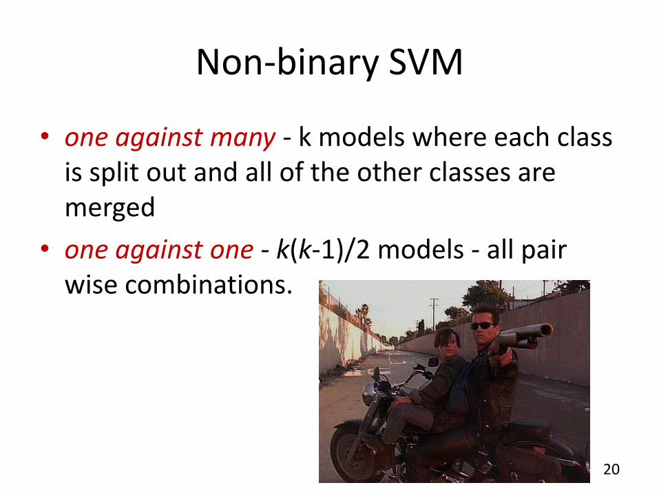
Non-binary SVM
• one against many - k models where each class is split out and all of the other classes are merged
• one against one - k(k-1)/2 models - all pair wise combinations.

21
What you have to do

22
SVM Tradeoffs
Advantages
• Hypothesis has an explicit dependence on data (support vectors)
• Few tuning parameters
Disadvantages
• No clear estimate of “confidence” to go along with classification. Next: A probabilistic model…
23
Bayesian Learner

24
A Probabilistic Classifier
• What’s the probability of class C, given feature vector x?
• The problem: If features can take on r different values, there are rn different probabilities to consider!
• Bayes’ Theorem to the rescue…
)|( ,1 nxxCP

25
Bayes’ Theorem
• Bayes' theorem describes the way in which one's beliefs about observing 'A' are updated by having observed 'B'.
)(
)()|()|(
BP
APABPBAP
26
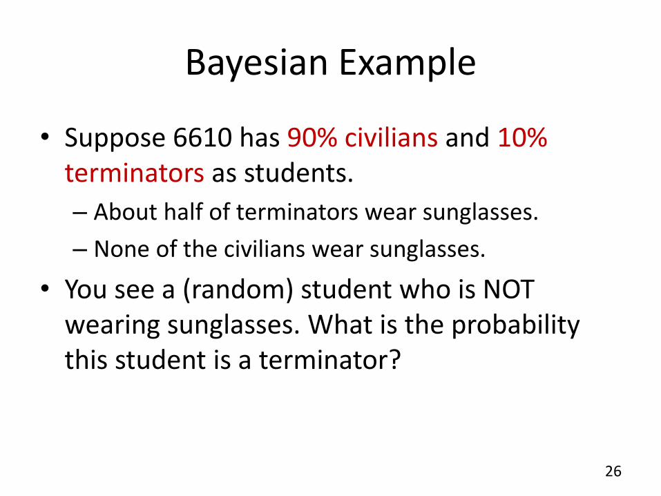
Bayesian Example
• Suppose 6610 has 90% civilians and 10% terminators as students.
– About half of terminators wear sunglasses.
– None of the civilians wear sunglasses.
• You see a (random) student who is NOT wearing sunglasses. What is the probability this student is a terminator?
27
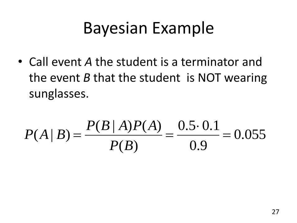
Bayesian Example
• Call event A the student is a terminator and the event B that the student is NOT wearing sunglasses.
055.09.0
1.05.0
)(
)()|()|(
BP
APABPBAP

28
Applying Bayes’ Theorem to ML
• Denominator is effectively constant.
• Assuming conditional independence
• We can say:
)(
)|()()|(
,1
,1
,1
n
n
nxxP
CxxPCPxxCP
)|()|()|,( CxPCxPCxxP jiji
n
i
in CxPCPxxCP1
,1 )|()()|(
29
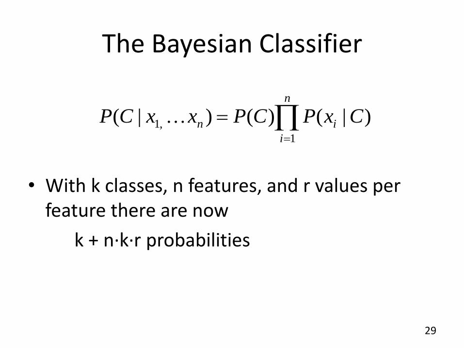
The Bayesian Classifier
• With k classes, n features, and r values per feature there are now
k + n∙k∙r probabilities
n
i
in CxPCPxxCP1
,1 )|()()|(

30
Bayesian Advantages
• Fast to train, fast to classify
• Well suited for nominal features
• Good for combining models:
– Suppose we have two kinds of feature vectors, x1 and x2 Rather than building a monolithic model, it might be more practical to learn two separate classifiers, P(C|x1) and P(C|x2) and then to combine them.
)(
)|()|(),|( 21
21CP
xCPxCPxxCP
31
Bayesian Disadvantages
• If conditional independence isn’t true (at least most of the time), it may not make for a very good model

32
Advanced ML Algorithms
• Support Vector Machines
• Bayesian
• Decision Trees
• Artificial Neural Networks

33
Decision Trees

34
Automatic Decision Tree Building
• Most algorithms are variations on a top-down, greedy search through the space of possible decision trees.
• Search through the attributes of the training instances and pick the attribute that best separates the given examples.
• If the attribute perfectly classifies the training sets then stop.
• Otherwise recursively operate on the partitioned subsets to get their "best" attribute.

35
Decision Tree Advantages
• Simple to understand and interpret.
• Able to handle both numerical and categorical data.
• Possible to validate a model using statistical tests. That makes it possible to account for the reliability of the model.
• Decisions are fast

36
Artificial Neural Networks

37
ANNs • Idea: simulate biological neural networks
• Learning occurs by changing the effectiveness of the synapses so that the influence of one neuron on another changes.
38
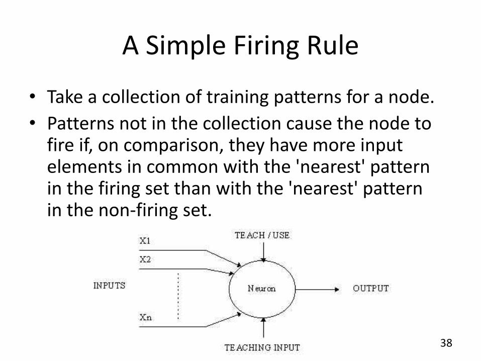
A Simple Firing Rule
• Take a collection of training patterns for a node.
• Patterns not in the collection cause the node to fire if, on comparison, they have more input elements in common with the 'nearest' pattern in the firing set than with the 'nearest' pattern in the non-firing set.

39
A More Complicated Neuron
• Weight the inputs.
• These weighted inputs are then added together and if they exceed a pre-set threshold value, the neuron fires. In any other case the neuron does not fire.

40
Multilayer Neural Net
41
ANN Success Stories
• Handwriting recognition
• Recognizing spoken words
• Face recognition
• ALVINN
• TD-BACKGAMMON

42
ALVINN
• Autonomous Land Vehicle
in a Neural Network
• 1995 – Drove 1000 miles in traffic at speed of
up to 120 MPH
– Steered the car coast to coast (throttle and brakes controlled by human)
• 30 x 32 image as input, 4 hidden units, and 30 outputs

43
TD-GAMMON
• Plays backgammon
• Created by Gerry Tesauro in the early 90s
• Uses variation of Q-learning
– Neural network was used to learn the evaluation function
• Trained on over 1 million games played against itself
• Plays competitively at world class level

44
ANN Advantages
• Online learning
• Large dataset applications
• Their simple implementation and the existence of mostly local dependencies exhibited in the structure allows for fast, parallel implementations in hardware.

45
ANN Disadvantages
• Model is opaque
• Can take a long time to train
• Have to re-train whole thing when new features are added
46
You must choose…
How would you design a …
1. Spam Filter
2. Alarm system for a nuclear power plant
3. Terminator (Learn to act like a human, terminate John Connor)

47
Boosting
Can a set of weak learners create a single strong learner?
• Weak learner: classifier which is only slightly correlated with the true classification.
• Strong learner: a classifier that is arbitrarily well-correlated with the true classification.
• Most boosting algorithms consist of iteratively weighting weak learners in some way that is usually related to the weak learner's accuracy.
• After a weak learner is added, the data is reweighted: examples that are misclassified gain weight and examples that are classified correctly lose weight.

48
Boosting & Cake Eating
• Can only work when the different learners have learned different things
• Combining is non-trivial
• Boosted decision trees a probably most popular

49
Now: Practical Stuff
• Features (find, selecting, etc.)
• Evaluating a model
• External Validity
• Other things to think about
• Where to go for code etc.
50
Features

51
Forming a model
• ML is a recipe for solving a certain type of problem:
• Trick is to formulate a predictive model by choosing the right “features”
},),({ YyXxyx
FfYXf ,:
,: FC

52

53
Features /**
* Moves this unit to america.
*
* @exception IllegalStateException If the
move is illegal.
*/
public void moveToAmerica() {
if (!(getLocation() instanceof Europe))
{
throw new IllegalStateException("A
unit can only be "
+ "moved to america from
europe.");
}
setState(TO_AMERICA);
// Clear the alreadyOnHighSea flag
alreadyOnHighSea = false;
}
feature value
Comments 2
Function calls 3
LOC 19
Has Exception? TRUE

54
Feature Importance
• Often we want to understand which features are most predictive
• Three Basic Techniques
– Inspect Model Directly (Not always possible)
– Leave-one-out analysis (Train on all features but one)
– Singleton feature analysis (Train on each feature individually)

55
Feature Importance Example

56
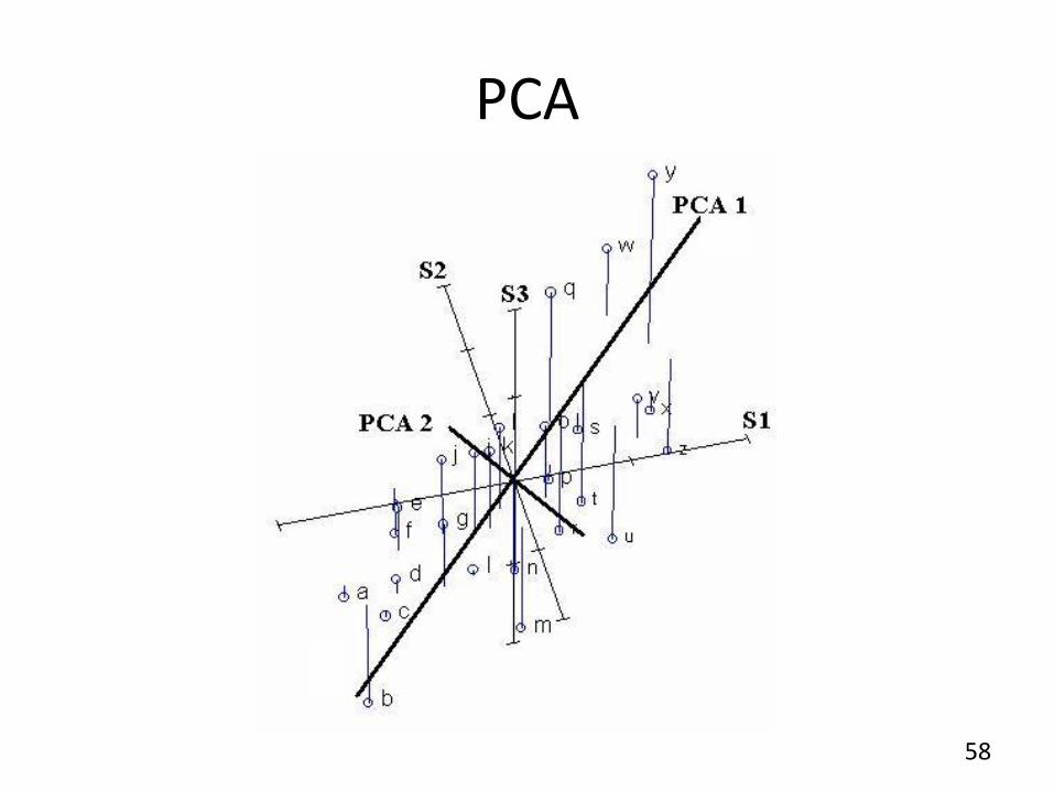
When Features Overlap
• Sometimes we want to know how many features are actually needed
• Example: – Feature 1: Lines of code
– Feature 2: Lines of code ∙ 2
• Solution: Principle Component Analysis (PCA)
• Idea: Iteratively perform linear regressions, find out how many vectors (ideal features) are needed to account for variance in the data.

57
PCA
58
PCA

59
PCA
• Each PC reduces dimensionality such that the total linear variability is reduced
• Repeat until no dimensions left
• Can only account for linear variability
60
Curse of Dimensionality
• More features is NOT always “more better”
• Problems tend to become intractable as number of variables increases
• Data spreads out exponentially with the number of dimensions (makes data sparse in high dimensions)
• Makes any kind of attempt to search, sort, filter or organize nearly impossible as you will have no way to compare two items in your data set with values along mostly disjoint sets of variables.

61
Feature Selection
• Alleviating the curse of dimensionality
• Enhances generalization capability
• Speeds up learning process
• Improves model interpretability

62
Feature Selection
• Optimal feature selection requires an exhaustive search of all possible subsets of features of size N
• Feature ranking: rank the features by a metric and choose the top N
• Stepwise Regression: Greedy algorithm that adds the best feature (or deletes the worst feature) at each round until N are left.

63
Evaluation

64
Direct Model Evaluation
• How closely does the model conform to the data?
• This is non-trivial
• Major Issues
– Bias
– Statistical Significance
– Over-fitting

65
Evaluation Strategy 1: Correlation
• Suppose we have a vector of correct answers X, and model output Y
• Question: How similar are X and Y?
• Pearson Product Moment Correlation Coefficient : r
• If r2 is 0.90, then 90% of the variance of Y can be “explained" by the linear relationship between X and Y
• But what if the data is categorical?

66
Evaluation Strategy 2: f-measure
• You have a binary classifier for “will this report be resolved in <= 30 days”
• You have 27,984 reports with known answers – C = correct set of reports resolved in 30 days
– R = set of reports the model returns
Precision = Recall =
f-measure=
||
||
R
RC
||
||
C
RC
RP
RP
2

67
f-measure and Bias
• Say you have 100 instances • 50 yes instances, 50 no instances, at random
– “Flip Fair Coin”: Prec=0.5, Rec=0.5, F=0.5 – “Always Guess Yes”: Prec=0.5, Rec=1.0, F=0.66
• 70 yes instances, 30 no instances, at random – “Flip Fair Coin”: Prec=0.7, Rec=0.5, F=0.58 – “Flip Biased Coin”: Prec=0.7, Rec=0.7, F=0.7 – “Always Guess Yes”: Prec=0.7, Rec=1.0, F=0.82
• May want to subsample to 50-50 split for evaluation purposes

68
Other accuracy metrics
• % of instances correctly classified
• Cohen’s Kappa
• Root mean squared error

69

70
Cross Validation to test for over-fitting
• Idea: Don’t evaluate on the same data you trained on.
• N-Fold Cross-Validation
– Partition instances into n subsets
– Train on 2..n and test on 1
– Train on 1, 3..n and test on 2, etc.

71
External Validity
• Sometimes we want to explore how well a model correlates with some external truth (e.g., to show utility)
• Solution:
– Discrete Case: f-measure
– Continuous Case: Pearson
– Hybrid: Bins + Kendall’s Tau

72
Even More Practical
ML implementations available in the environment of your choice
• Matlab
• R
• Weka (Java)
• Mathmatica
• [Many others]

73
The End?


