

Regression Basis Functions Loss Functions Weights Regularization Bayesian
Linear Models for RegressionMachine Learning
Torsten Möller
©Möller/Mori 1

Regression Basis Functions Loss Functions Weights Regularization Bayesian
Reading
• Chapter 3 of “Pattern Recognition and Machine Learning” byBishop
• Chapter 3+5+6+7 of “The Elements of Statistical Learning”by Hastie, Tibshirani, Friedman
©Möller/Mori 2
Regression Basis Functions Loss Functions Weights Regularization Bayesian
Outline
Regression
Linear Basis Function Models
Loss Functions for Regression
Finding Optimal Weights
Regularization
Bayesian Linear Regression
©Möller/Mori 3

Regression Basis Functions Loss Functions Weights Regularization Bayesian
Outline
Regression
Linear Basis Function Models
Loss Functions for Regression
Finding Optimal Weights
Regularization
Bayesian Linear Regression
©Möller/Mori 4
Regression Basis Functions Loss Functions Weights Regularization Bayesian
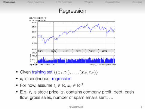
Regression
• Given training set {(x1, t1), . . . , (xN , tN )}• ti is continuous: regression• For now, assume ti ∈ R, xi ∈ RD
• E.g. ti is stock price, xi contains company profit, debt, cashflow, gross sales, number of spam emails sent, …
©Möller/Mori 5
Regression Basis Functions Loss Functions Weights Regularization Bayesian
Outline
Regression
Linear Basis Function Models
Loss Functions for Regression
Finding Optimal Weights
Regularization
Bayesian Linear Regression
©Möller/Mori 6

Regression Basis Functions Loss Functions Weights Regularization Bayesian
Linear Functions
• A function f(·) is linear if
f(αx1 + βx2) = αf(x1) + βf(x2)
• Linear functions will lead to simple algorithms, so let’s seewhat we can do with them
©Möller/Mori 7
Regression Basis Functions Loss Functions Weights Regularization Bayesian
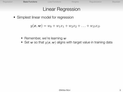
Linear Regression• Simplest linear model for regression
y(x,w) = w0 + w1x1 + w2x2 + . . .+ wDxD
• Remember, we’re learning w• Set w so that y(x,w) aligns with target value in training data
• This is a very simple model, limited in what it can do
�
�
�����
0 1
−1
0
1
©Möller/Mori 8
Regression Basis Functions Loss Functions Weights Regularization Bayesian
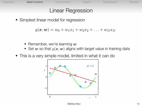
Linear Regression• Simplest linear model for regression
y(x,w) = w0 + w1x1 + w2x2 + . . .+ wDxD
• Remember, we’re learning w• Set w so that y(x,w) aligns with target value in training data
• This is a very simple model, limited in what it can do
�
�
�����
0 1
−1
0
1
©Möller/Mori 9
Regression Basis Functions Loss Functions Weights Regularization Bayesian
Linear Regression• Simplest linear model for regression
y(x,w) = w0 + w1x1 + w2x2 + . . .+ wDxD
• Remember, we’re learning w• Set w so that y(x,w) aligns with target value in training data
• This is a very simple model, limited in what it can do
�
�
�����
0 1
−1
0
1
©Möller/Mori 10
Regression Basis Functions Loss Functions Weights Regularization Bayesian
Linear Basis Function Models
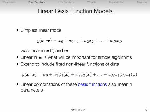
• Simplest linear model
y(x,w) = w0 + w1x1 + w2x2 + . . .+ wDxD
was linear in x (∗) and w
• Linear in w is what will be important for simple algorithms• Extend to include fixed non-linear functions of data
y(x,w) = w0 + w1ϕ1(x) + w2ϕ2(x) + . . .+ wM−1ϕM−1(x)
• Linear combinations of these basis functions also linear inparameters
©Möller/Mori 11
Regression Basis Functions Loss Functions Weights Regularization Bayesian
Linear Basis Function Models
• Simplest linear model
y(x,w) = w0 + w1x1 + w2x2 + . . .+ wDxD
was linear in x (∗) and w
• Linear in w is what will be important for simple algorithms• Extend to include fixed non-linear functions of data
y(x,w) = w0 + w1ϕ1(x) + w2ϕ2(x) + . . .+ wM−1ϕM−1(x)
• Linear combinations of these basis functions also linear inparameters
©Möller/Mori 12
Regression Basis Functions Loss Functions Weights Regularization Bayesian
Linear Basis Function Models
• Simplest linear model
y(x,w) = w0 + w1x1 + w2x2 + . . .+ wDxD
was linear in x (∗) and w
• Linear in w is what will be important for simple algorithms• Extend to include fixed non-linear functions of data
y(x,w) = w0 + w1ϕ1(x) + w2ϕ2(x) + . . .+ wM−1ϕM−1(x)
• Linear combinations of these basis functions also linear inparameters
©Möller/Mori 13
Regression Basis Functions Loss Functions Weights Regularization Bayesian
Linear Basis Function Models
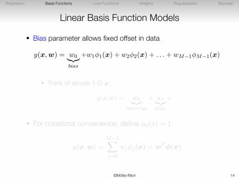
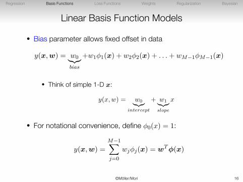
• Bias parameter allows fixed offset in data
y(x,w) = w0︸︷︷︸bias
+w1ϕ1(x) + w2ϕ2(x) + . . .+ wM−1ϕM−1(x)
• Think of simple 1-D x:
y(x,w) = w0︸︷︷︸intercept
+ w1︸︷︷︸slope
x
• For notational convenience, define ϕ0(x) = 1:
y(x,w) =
M−1∑j=0
wjϕj(x) = wTϕ(x)
©Möller/Mori 14

Regression Basis Functions Loss Functions Weights Regularization Bayesian
Linear Basis Function Models
• Bias parameter allows fixed offset in data
y(x,w) = w0︸︷︷︸bias
+w1ϕ1(x) + w2ϕ2(x) + . . .+ wM−1ϕM−1(x)
• Think of simple 1-D x:
y(x,w) = w0︸︷︷︸intercept
+ w1︸︷︷︸slope
x
• For notational convenience, define ϕ0(x) = 1:
y(x,w) =
M−1∑j=0
wjϕj(x) = wTϕ(x)
©Möller/Mori 15
Regression Basis Functions Loss Functions Weights Regularization Bayesian
Linear Basis Function Models
• Bias parameter allows fixed offset in data
y(x,w) = w0︸︷︷︸bias
+w1ϕ1(x) + w2ϕ2(x) + . . .+ wM−1ϕM−1(x)
• Think of simple 1-D x:
y(x,w) = w0︸︷︷︸intercept
+ w1︸︷︷︸slope
x
• For notational convenience, define ϕ0(x) = 1:
y(x,w) =
M−1∑j=0
wjϕj(x) = wTϕ(x)
©Möller/Mori 16
Regression Basis Functions Loss Functions Weights Regularization Bayesian
Linear Basis Function Models
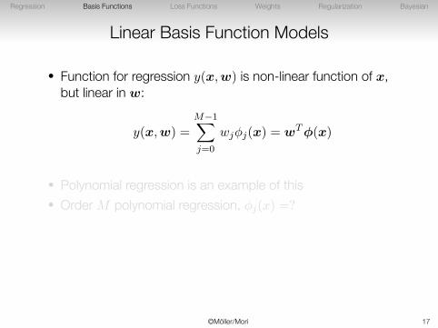
• Function for regression y(x,w) is non-linear function of x,but linear in w:
y(x,w) =M−1∑j=0
wjϕj(x) = wTϕ(x)
• Polynomial regression is an example of this• Order M polynomial regression, ϕj(x) =?
• ϕj(x) = xj :
y(x,w) = w0x0 + w1x
1 + . . .+ wMxM
©Möller/Mori 17

Regression Basis Functions Loss Functions Weights Regularization Bayesian
Linear Basis Function Models
• Function for regression y(x,w) is non-linear function of x,but linear in w:
y(x,w) =M−1∑j=0
wjϕj(x) = wTϕ(x)
• Polynomial regression is an example of this• Order M polynomial regression, ϕj(x) =?
• ϕj(x) = xj :
y(x,w) = w0x0 + w1x
1 + . . .+ wMxM
©Möller/Mori 18

Regression Basis Functions Loss Functions Weights Regularization Bayesian
Linear Basis Function Models
• Function for regression y(x,w) is non-linear function of x,but linear in w:
y(x,w) =M−1∑j=0
wjϕj(x) = wTϕ(x)
• Polynomial regression is an example of this• Order M polynomial regression, ϕj(x) =?
• ϕj(x) = xj :
y(x,w) = w0x0 + w1x
1 + . . .+ wMxM
©Möller/Mori 19
Regression Basis Functions Loss Functions Weights Regularization Bayesian
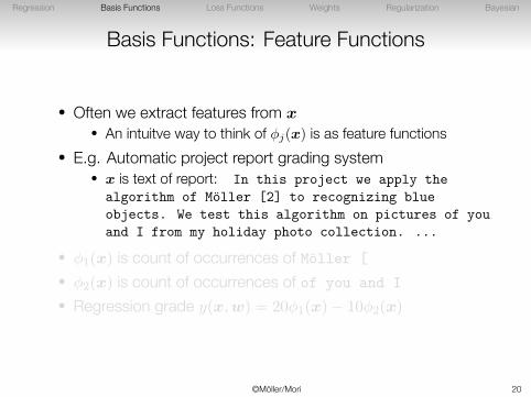
Basis Functions: Feature Functions
• Often we extract features from x• An intuitve way to think of ϕj(x) is as feature functions
• E.g. Automatic project report grading system• x is text of report: In this project we apply the
algorithm of Möller [2] to recognizing blueobjects. We test this algorithm on pictures of youand I from my holiday photo collection. ...
• ϕ1(x) is count of occurrences of Möller [• ϕ2(x) is count of occurrences of of you and I• Regression grade y(x,w) = 20ϕ1(x)− 10ϕ2(x)
©Möller/Mori 20

Regression Basis Functions Loss Functions Weights Regularization Bayesian
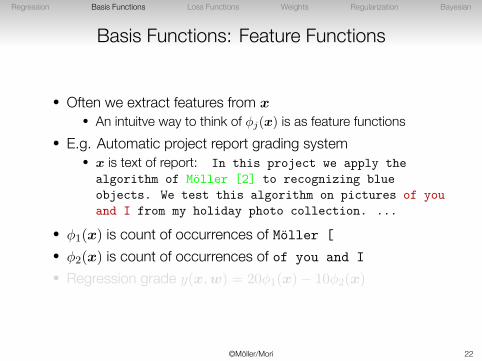
Basis Functions: Feature Functions
• Often we extract features from x• An intuitve way to think of ϕj(x) is as feature functions
• E.g. Automatic project report grading system• x is text of report: In this project we apply the
algorithm of Möller [2] to recognizing blueobjects. We test this algorithm on pictures of youand I from my holiday photo collection. ...
• ϕ1(x) is count of occurrences of Möller [• ϕ2(x) is count of occurrences of of you and I• Regression grade y(x,w) = 20ϕ1(x)− 10ϕ2(x)
©Möller/Mori 21
Regression Basis Functions Loss Functions Weights Regularization Bayesian
Basis Functions: Feature Functions
• Often we extract features from x• An intuitve way to think of ϕj(x) is as feature functions
• E.g. Automatic project report grading system• x is text of report: In this project we apply the
algorithm of Möller [2] to recognizing blueobjects. We test this algorithm on pictures of youand I from my holiday photo collection. ...
• ϕ1(x) is count of occurrences of Möller [• ϕ2(x) is count of occurrences of of you and I• Regression grade y(x,w) = 20ϕ1(x)− 10ϕ2(x)
©Möller/Mori 22

Regression Basis Functions Loss Functions Weights Regularization Bayesian
Basis Functions: Feature Functions
• Often we extract features from x• An intuitve way to think of ϕj(x) is as feature functions
• E.g. Automatic project report grading system• x is text of report: In this project we apply the
algorithm of Möller [2] to recognizing blueobjects. We test this algorithm on pictures of youand I from my holiday photo collection. ...
• ϕ1(x) is count of occurrences of Möller [• ϕ2(x) is count of occurrences of of you and I• Regression grade y(x,w) = 20ϕ1(x)− 10ϕ2(x)
©Möller/Mori 23
Regression Basis Functions Loss Functions Weights Regularization Bayesian
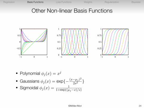
Other Non-linear Basis Functions
−1 0 1−1
−0.5
0
0.5
1
−1 0 10
0.25
0.5
0.75
1
−1 0 10
0.25
0.5
0.75
1
• Polynomial ϕj(x) = xj
• Gaussians ϕj(x) = exp{− (x−µj)2
2s2}
• Sigmoidal ϕj(x) =1
1+exp((µj−x)/s)
©Möller/Mori 24
Regression Basis Functions Loss Functions Weights Regularization Bayesian
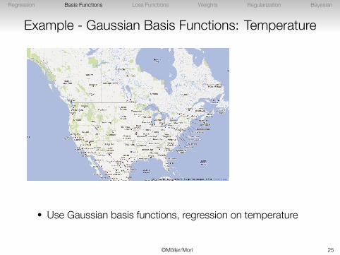
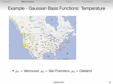
Example - Gaussian Basis Functions: Temperature
• Use Gaussian basis functions, regression on temperature
©Möller/Mori 25
Regression Basis Functions Loss Functions Weights Regularization Bayesian
Example - Gaussian Basis Functions: Temperature
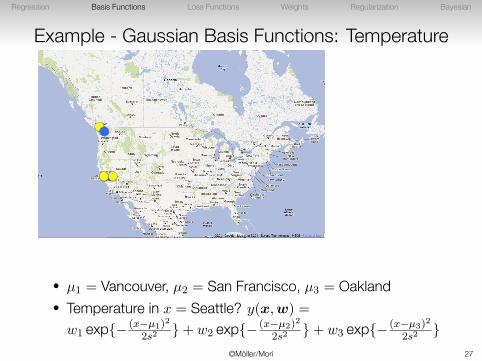
• µ1 = Vancouver, µ2 = San Francisco, µ3 = Oakland
©Möller/Mori 26
Regression Basis Functions Loss Functions Weights Regularization Bayesian
Example - Gaussian Basis Functions: Temperature
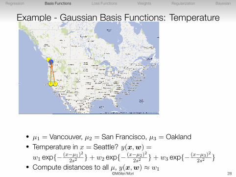
• µ1 = Vancouver, µ2 = San Francisco, µ3 = Oakland• Temperature in x = Seattle? y(x,w) =
w1 exp{− (x−µ1)2
2s2}+ w2 exp{− (x−µ2)2
2s2}+ w3 exp{− (x−µ3)2
2s2}
©Möller/Mori 27
Regression Basis Functions Loss Functions Weights Regularization Bayesian
Example - Gaussian Basis Functions: Temperature
• µ1 = Vancouver, µ2 = San Francisco, µ3 = Oakland• Temperature in x = Seattle? y(x,w) =
w1 exp{− (x−µ1)2
2s2}+ w2 exp{− (x−µ2)2
2s2}+ w3 exp{− (x−µ3)2
2s2}
• Compute distances to all µ, y(x,w) ≈ w1©Möller/Mori 28

Regression Basis Functions Loss Functions Weights Regularization Bayesian
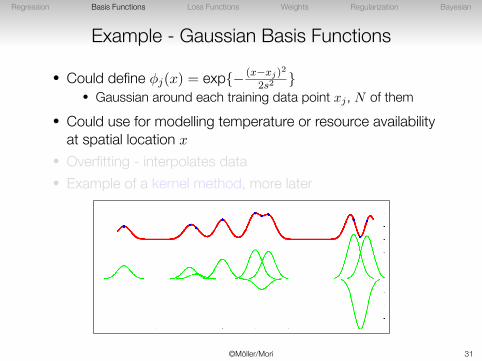
Example - Gaussian Basis Functions
• Could define ϕj(x) = exp{− (x−xj)2
2s2}
• Gaussian around each training data point xj , N of them• Could use for modelling temperature or resource availability
at spatial location x
• Overfitting - interpolates data• Example of a kernel method, more later
©Möller/Mori 29
Regression Basis Functions Loss Functions Weights Regularization Bayesian
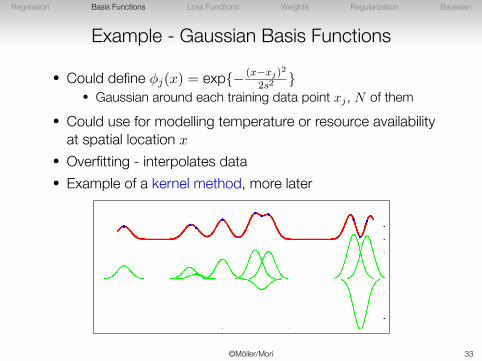
Example - Gaussian Basis Functions
• Could define ϕj(x) = exp{− (x−xj)2
2s2}
• Gaussian around each training data point xj , N of them• Could use for modelling temperature or resource availability
at spatial location x
• Overfitting - interpolates data• Example of a kernel method, more later
©Möller/Mori 30
Regression Basis Functions Loss Functions Weights Regularization Bayesian
Example - Gaussian Basis Functions
• Could define ϕj(x) = exp{− (x−xj)2
2s2}
• Gaussian around each training data point xj , N of them• Could use for modelling temperature or resource availability
at spatial location x
• Overfitting - interpolates data• Example of a kernel method, more later
©Möller/Mori 31

Regression Basis Functions Loss Functions Weights Regularization Bayesian
Example - Gaussian Basis Functions
• Could define ϕj(x) = exp{− (x−xj)2
2s2}
• Gaussian around each training data point xj , N of them• Could use for modelling temperature or resource availability
at spatial location x
• Overfitting - interpolates data• Example of a kernel method, more later
©Möller/Mori 32
Regression Basis Functions Loss Functions Weights Regularization Bayesian
Example - Gaussian Basis Functions
• Could define ϕj(x) = exp{− (x−xj)2
2s2}
• Gaussian around each training data point xj , N of them• Could use for modelling temperature or resource availability
at spatial location x
• Overfitting - interpolates data• Example of a kernel method, more later
©Möller/Mori 33

Regression Basis Functions Loss Functions Weights Regularization Bayesian
Outline
Regression
Linear Basis Function Models
Loss Functions for Regression
Finding Optimal Weights
Regularization
Bayesian Linear Regression
©Möller/Mori 34
Regression Basis Functions Loss Functions Weights Regularization Bayesian
Loss Functions for Regression
• We want to find the “best” set of coefficients w
• Recall, one way to define “best” was minimizing squarederror:
E(w) =1
2
N∑n=1
{y(xn,w)− tn}2
• We will now look at another way, based on maximumlikelihood
©Möller/Mori 35

Regression Basis Functions Loss Functions Weights Regularization Bayesian
Gaussian Noise Model for Regression
• We are provided with a training set {(xi, ti)}• Let’s assume t arises from a deterministic function plus
Gaussian distributed (with precision β) noise:
t = y(x,w) + ϵ
• The probability of observing a target value t is then:
p(t|x,w, β) = N (t|y(x,w), β−1)
• Notation: N (x|µ, σ2); x drawn from Gaussian with mean µ,variance σ2
©Möller/Mori 36

Regression Basis Functions Loss Functions Weights Regularization Bayesian
Gaussian Noise Model for Regression
• We are provided with a training set {(xi, ti)}• Let’s assume t arises from a deterministic function plus
Gaussian distributed (with precision β) noise:
t = y(x,w) + ϵ
• The probability of observing a target value t is then:
p(t|x,w, β) = N (t|y(x,w), β−1)
• Notation: N (x|µ, σ2); x drawn from Gaussian with mean µ,variance σ2
©Möller/Mori 37
Regression Basis Functions Loss Functions Weights Regularization Bayesian
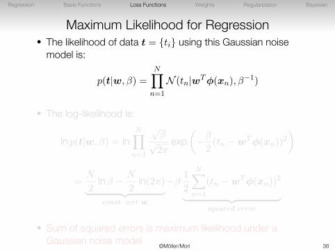
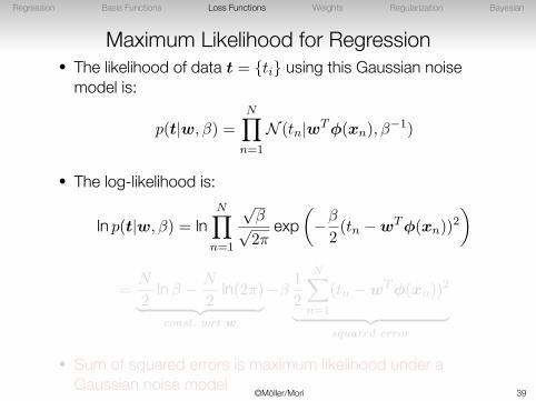
Maximum Likelihood for Regression• The likelihood of data t = {ti} using this Gaussian noise
model is:
p(t|w, β) =N∏
n=1
N (tn|wTϕ(xn), β−1)
• The log-likelihood is:
ln p(t|w, β) = lnN∏
n=1
√β√2π
exp(−β
2(tn −wTϕ(xn))
2
)
=N
2lnβ − N
2ln(2π)︸ ︷︷ ︸
const. wrt w
−β1
2
N∑n=1
(tn −wTϕ(xn))2
︸ ︷︷ ︸squared error
• Sum of squared errors is maximum likelihood under aGaussian noise model ©Möller/Mori 38
Regression Basis Functions Loss Functions Weights Regularization Bayesian
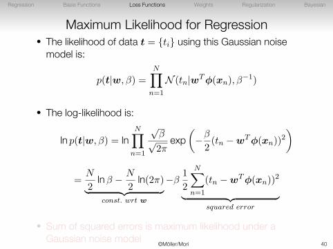
Maximum Likelihood for Regression• The likelihood of data t = {ti} using this Gaussian noise
model is:
p(t|w, β) =N∏
n=1
N (tn|wTϕ(xn), β−1)
• The log-likelihood is:
ln p(t|w, β) = lnN∏
n=1
√β√2π
exp(−β
2(tn −wTϕ(xn))
2
)
=N
2lnβ − N
2ln(2π)︸ ︷︷ ︸
const. wrt w
−β1
2
N∑n=1
(tn −wTϕ(xn))2
︸ ︷︷ ︸squared error
• Sum of squared errors is maximum likelihood under aGaussian noise model ©Möller/Mori 39
Regression Basis Functions Loss Functions Weights Regularization Bayesian
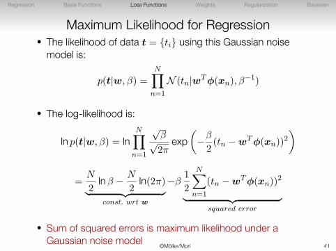
Maximum Likelihood for Regression• The likelihood of data t = {ti} using this Gaussian noise
model is:
p(t|w, β) =N∏
n=1
N (tn|wTϕ(xn), β−1)
• The log-likelihood is:
ln p(t|w, β) = lnN∏
n=1
√β√2π
exp(−β
2(tn −wTϕ(xn))
2
)
=N
2lnβ − N
2ln(2π)︸ ︷︷ ︸
const. wrt w
−β1
2
N∑n=1
(tn −wTϕ(xn))2
︸ ︷︷ ︸squared error
• Sum of squared errors is maximum likelihood under aGaussian noise model ©Möller/Mori 40
Regression Basis Functions Loss Functions Weights Regularization Bayesian
Maximum Likelihood for Regression• The likelihood of data t = {ti} using this Gaussian noise
model is:
p(t|w, β) =N∏
n=1
N (tn|wTϕ(xn), β−1)
• The log-likelihood is:
ln p(t|w, β) = lnN∏
n=1
√β√2π
exp(−β
2(tn −wTϕ(xn))
2
)
=N
2lnβ − N
2ln(2π)︸ ︷︷ ︸
const. wrt w
−β1
2
N∑n=1
(tn −wTϕ(xn))2
︸ ︷︷ ︸squared error
• Sum of squared errors is maximum likelihood under aGaussian noise model ©Möller/Mori 41
Regression Basis Functions Loss Functions Weights Regularization Bayesian
Outline
Regression
Linear Basis Function Models
Loss Functions for Regression
Finding Optimal Weights
Regularization
Bayesian Linear Regression
©Möller/Mori 42

Regression Basis Functions Loss Functions Weights Regularization Bayesian
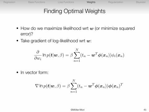
Finding Optimal Weights
• How do we maximize likelihood wrt w (or minimize squarederror)?
• Take gradient of log-likelihood wrt w:
∂
∂wiln p(t|w, β) = β
N∑n=1
(tn −wTϕ(xn))ϕi(xn)
• In vector form:
∇ ln p(t|w, β) = βN∑
n=1
(tn −wTϕ(xn))ϕ(xn)T
©Möller/Mori 43

Regression Basis Functions Loss Functions Weights Regularization Bayesian
Finding Optimal Weights
• How do we maximize likelihood wrt w (or minimize squarederror)?
• Take gradient of log-likelihood wrt w:
∂
∂wiln p(t|w, β) = β
N∑n=1
(tn −wTϕ(xn))ϕi(xn)
• In vector form:
∇ ln p(t|w, β) = βN∑
n=1
(tn −wTϕ(xn))ϕ(xn)T
©Möller/Mori 44
Regression Basis Functions Loss Functions Weights Regularization Bayesian
Finding Optimal Weights
• How do we maximize likelihood wrt w (or minimize squarederror)?
• Take gradient of log-likelihood wrt w:
∂
∂wiln p(t|w, β) = β
N∑n=1
(tn −wTϕ(xn))ϕi(xn)
• In vector form:
∇ ln p(t|w, β) = βN∑
n=1
(tn −wTϕ(xn))ϕ(xn)T
©Möller/Mori 45
Regression Basis Functions Loss Functions Weights Regularization Bayesian
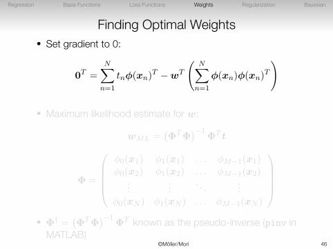
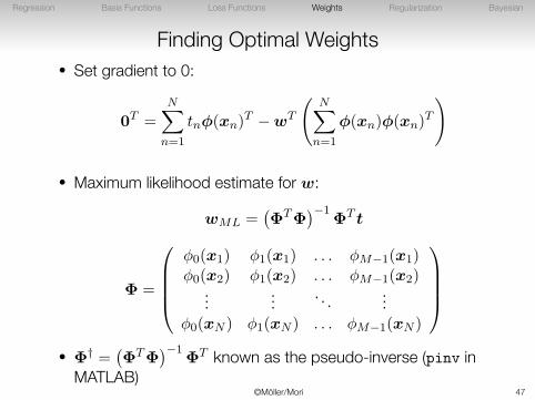
Finding Optimal Weights• Set gradient to 0:
0T =
N∑n=1
tnϕ(xn)T −wT
(N∑
n=1
ϕ(xn)ϕ(xn)T
)
• Maximum likelihood estimate for w:
wML =(ΦTΦ
)−1ΦT t
Φ =
ϕ0(x1) ϕ1(x1) . . . ϕM−1(x1)ϕ0(x2) ϕ1(x2) . . . ϕM−1(x2)
...... . . . ...
ϕ0(xN ) ϕ1(xN ) . . . ϕM−1(xN )
• Φ† =
(ΦTΦ
)−1ΦT known as the pseudo-inverse (pinv in
MATLAB)©Möller/Mori 46
Regression Basis Functions Loss Functions Weights Regularization Bayesian
Finding Optimal Weights• Set gradient to 0:
0T =
N∑n=1
tnϕ(xn)T −wT
(N∑
n=1
ϕ(xn)ϕ(xn)T
)
• Maximum likelihood estimate for w:
wML =(ΦTΦ
)−1ΦT t
Φ =
ϕ0(x1) ϕ1(x1) . . . ϕM−1(x1)ϕ0(x2) ϕ1(x2) . . . ϕM−1(x2)
...... . . . ...
ϕ0(xN ) ϕ1(xN ) . . . ϕM−1(xN )
• Φ† =
(ΦTΦ
)−1ΦT known as the pseudo-inverse (pinv in
MATLAB)©Möller/Mori 47
Regression Basis Functions Loss Functions Weights Regularization Bayesian
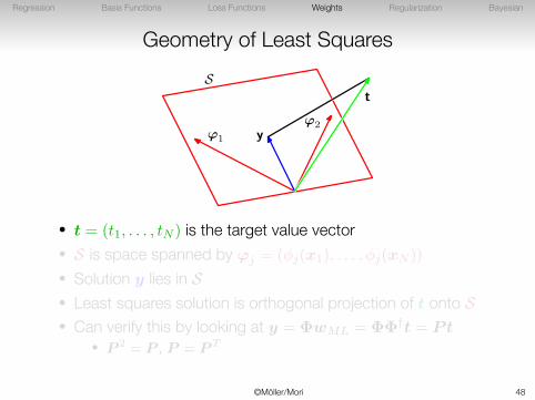
Geometry of Least SquaresS
t
yϕ1
ϕ2
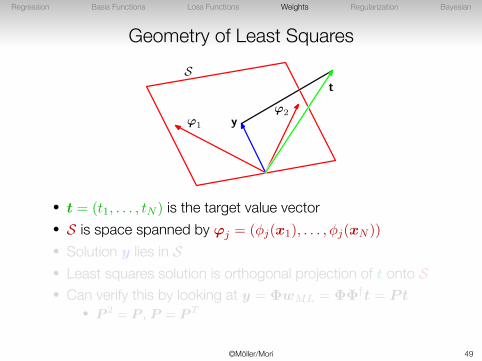
• t = (t1, . . . , tN ) is the target value vector• S is space spanned by φj = (ϕj(x1), . . . , ϕj(xN ))
• Solution y lies in S• Least squares solution is orthogonal projection of t onto S• Can verify this by looking at y = ΦwML = ΦΦ†t = Pt
• P 2 = P , P = P T
©Möller/Mori 48
Regression Basis Functions Loss Functions Weights Regularization Bayesian
Geometry of Least SquaresS
t
yϕ1
ϕ2
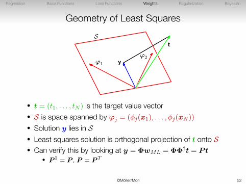
• t = (t1, . . . , tN ) is the target value vector• S is space spanned by φj = (ϕj(x1), . . . , ϕj(xN ))
• Solution y lies in S• Least squares solution is orthogonal projection of t onto S• Can verify this by looking at y = ΦwML = ΦΦ†t = Pt
• P 2 = P , P = P T
©Möller/Mori 49

Regression Basis Functions Loss Functions Weights Regularization Bayesian
Geometry of Least SquaresS
t
yϕ1
ϕ2
• t = (t1, . . . , tN ) is the target value vector• S is space spanned by φj = (ϕj(x1), . . . , ϕj(xN ))
• Solution y lies in S• Least squares solution is orthogonal projection of t onto S• Can verify this by looking at y = ΦwML = ΦΦ†t = Pt
• P 2 = P , P = P T
©Möller/Mori 50

Regression Basis Functions Loss Functions Weights Regularization Bayesian
Geometry of Least SquaresS
t
yϕ1
ϕ2
• t = (t1, . . . , tN ) is the target value vector• S is space spanned by φj = (ϕj(x1), . . . , ϕj(xN ))
• Solution y lies in S• Least squares solution is orthogonal projection of t onto S• Can verify this by looking at y = ΦwML = ΦΦ†t = Pt
• P 2 = P , P = P T
©Möller/Mori 51
Regression Basis Functions Loss Functions Weights Regularization Bayesian
Geometry of Least SquaresS
t
yϕ1
ϕ2
• t = (t1, . . . , tN ) is the target value vector• S is space spanned by φj = (ϕj(x1), . . . , ϕj(xN ))
• Solution y lies in S• Least squares solution is orthogonal projection of t onto S• Can verify this by looking at y = ΦwML = ΦΦ†t = Pt
• P 2 = P , P = P T
©Möller/Mori 52
Regression Basis Functions Loss Functions Weights Regularization Bayesian
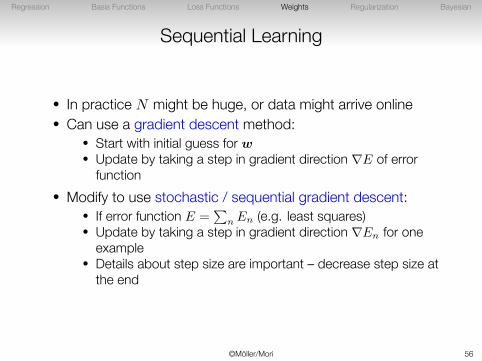
Sequential Learning
• In practice N might be huge, or data might arrive online• Can use a gradient descent method:
• Start with initial guess for w• Update by taking a step in gradient direction ∇E of error
function• Modify to use stochastic / sequential gradient descent:
• If error function E =∑
n En (e.g. least squares)• Update by taking a step in gradient direction ∇En for one
example• Details about step size are important – decrease step size at
the end
©Möller/Mori 53

Regression Basis Functions Loss Functions Weights Regularization Bayesian
Sequential Learning
• In practice N might be huge, or data might arrive online• Can use a gradient descent method:
• Start with initial guess for w• Update by taking a step in gradient direction ∇E of error
function• Modify to use stochastic / sequential gradient descent:
• If error function E =∑
n En (e.g. least squares)• Update by taking a step in gradient direction ∇En for one
example• Details about step size are important – decrease step size at
the end
©Möller/Mori 54
Regression Basis Functions Loss Functions Weights Regularization Bayesian
Sequential Learning
• In practice N might be huge, or data might arrive online• Can use a gradient descent method:
• Start with initial guess for w• Update by taking a step in gradient direction ∇E of error
function• Modify to use stochastic / sequential gradient descent:
• If error function E =∑
n En (e.g. least squares)• Update by taking a step in gradient direction ∇En for one
example• Details about step size are important – decrease step size at
the end
©Möller/Mori 55
Regression Basis Functions Loss Functions Weights Regularization Bayesian
Sequential Learning
• In practice N might be huge, or data might arrive online• Can use a gradient descent method:
• Start with initial guess for w• Update by taking a step in gradient direction ∇E of error
function• Modify to use stochastic / sequential gradient descent:
• If error function E =∑
n En (e.g. least squares)• Update by taking a step in gradient direction ∇En for one
example• Details about step size are important – decrease step size at
the end
©Möller/Mori 56
Regression Basis Functions Loss Functions Weights Regularization Bayesian
Outline
Regression
Linear Basis Function Models
Loss Functions for Regression
Finding Optimal Weights
Regularization
Bayesian Linear Regression
©Möller/Mori 57
Regression Basis Functions Loss Functions Weights Regularization Bayesian
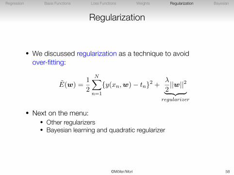
Regularization
• We discussed regularization as a technique to avoidover-fitting:
E(w) =1
2
N∑n=1
{y(xn,w)− tn}2 +λ
2||w||2︸ ︷︷ ︸
regularizer
• Next on the menu:• Other regularizers• Bayesian learning and quadratic regularizer
©Möller/Mori 58
Regression Basis Functions Loss Functions Weights Regularization Bayesian
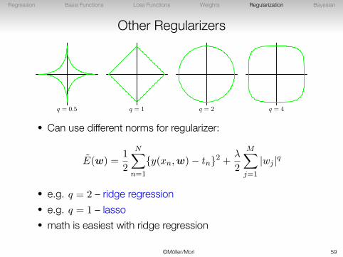
Other Regularizers
q = 0.5 q = 1 q = 2 q = 4
• Can use different norms for regularizer:
E(w) =1
2
N∑n=1
{y(xn,w)− tn}2 +λ
2
M∑j=1
|wj |q
• e.g. q = 2 – ridge regression• e.g. q = 1 – lasso• math is easiest with ridge regression
©Möller/Mori 59
Regression Basis Functions Loss Functions Weights Regularization Bayesian
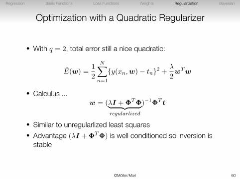
Optimization with a Quadratic Regularizer
• With q = 2, total error still a nice quadratic:
E(w) =1
2
N∑n=1
{y(xn,w)− tn}2 +λ
2wTw
• Calculus ...w = (λI +ΦTΦ︸ ︷︷ ︸
regularlized
)−1ΦT t
• Similar to unregularlized least squares• Advantage (λI +ΦTΦ) is well conditioned so inversion is
stable
©Möller/Mori 60
Regression Basis Functions Loss Functions Weights Regularization Bayesian
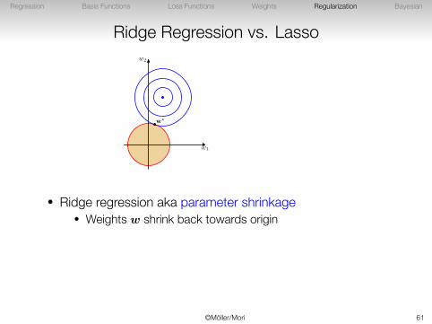
Ridge Regression vs. Lasso
w1
w2
w?
w1
w2
w?
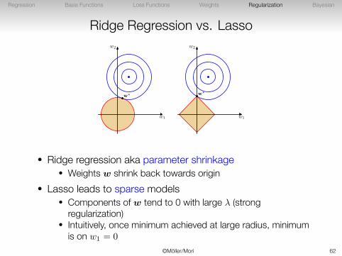
• Ridge regression aka parameter shrinkage• Weights w shrink back towards origin
• Lasso leads to sparse models• Components of w tend to 0 with large λ (strong
regularization)• Intuitively, once minimum achieved at large radius, minimum
is on w1 = 0
©Möller/Mori 61
Regression Basis Functions Loss Functions Weights Regularization Bayesian
Ridge Regression vs. Lasso
w1
w2
w?
w1
w2
w?
• Ridge regression aka parameter shrinkage• Weights w shrink back towards origin
• Lasso leads to sparse models• Components of w tend to 0 with large λ (strong
regularization)• Intuitively, once minimum achieved at large radius, minimum
is on w1 = 0
©Möller/Mori 62

Regression Basis Functions Loss Functions Weights Regularization Bayesian
Outline
Regression
Linear Basis Function Models
Loss Functions for Regression
Finding Optimal Weights
Regularization
Bayesian Linear Regression
©Möller/Mori 63
Regression Basis Functions Loss Functions Weights Regularization Bayesian
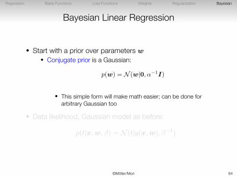
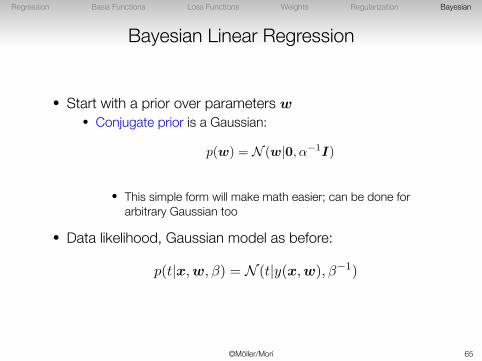
Bayesian Linear Regression
• Start with a prior over parameters w• Conjugate prior is a Gaussian:
p(w) = N (w|0, α−1I)
• This simple form will make math easier; can be done forarbitrary Gaussian too
• Data likelihood, Gaussian model as before:
p(t|x,w, β) = N (t|y(x,w), β−1)
©Möller/Mori 64
Regression Basis Functions Loss Functions Weights Regularization Bayesian
Bayesian Linear Regression
• Start with a prior over parameters w• Conjugate prior is a Gaussian:
p(w) = N (w|0, α−1I)
• This simple form will make math easier; can be done forarbitrary Gaussian too
• Data likelihood, Gaussian model as before:
p(t|x,w, β) = N (t|y(x,w), β−1)
©Möller/Mori 65
Regression Basis Functions Loss Functions Weights Regularization Bayesian
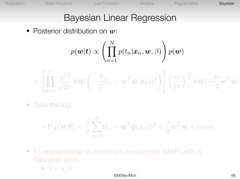
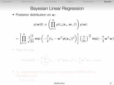
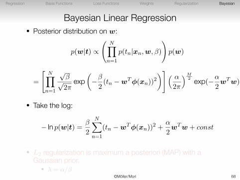
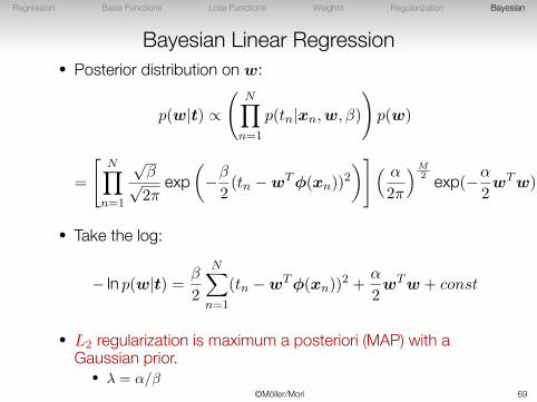
Bayesian Linear Regression• Posterior distribution on w:
p(w|t) ∝
(N∏
n=1
p(tn|xn,w, β)
)p(w)
=
[N∏
n=1
√β√2π
exp(−β
2(tn −wTϕ(xn))
2
)]( α
2π
)M2 exp(−α
2wTw)
• Take the log:
− ln p(w|t) = β
2
N∑n=1
(tn −wTϕ(xn))2 +
α
2wTw + const
• L2 regularization is maximum a posteriori (MAP) with aGaussian prior.
• λ = α/β©Möller/Mori 66
Regression Basis Functions Loss Functions Weights Regularization Bayesian
Bayesian Linear Regression• Posterior distribution on w:
p(w|t) ∝
(N∏
n=1
p(tn|xn,w, β)
)p(w)
=
[N∏
n=1
√β√2π
exp(−β
2(tn −wTϕ(xn))
2
)]( α
2π
)M2 exp(−α
2wTw)
• Take the log:
− ln p(w|t) = β
2
N∑n=1
(tn −wTϕ(xn))2 +
α
2wTw + const
• L2 regularization is maximum a posteriori (MAP) with aGaussian prior.
• λ = α/β©Möller/Mori 67
Regression Basis Functions Loss Functions Weights Regularization Bayesian
Bayesian Linear Regression• Posterior distribution on w:
p(w|t) ∝
(N∏
n=1
p(tn|xn,w, β)
)p(w)
=
[N∏
n=1
√β√2π
exp(−β
2(tn −wTϕ(xn))
2
)]( α
2π
)M2 exp(−α
2wTw)
• Take the log:
− ln p(w|t) = β
2
N∑n=1
(tn −wTϕ(xn))2 +
α
2wTw + const
• L2 regularization is maximum a posteriori (MAP) with aGaussian prior.
• λ = α/β©Möller/Mori 68
Regression Basis Functions Loss Functions Weights Regularization Bayesian
Bayesian Linear Regression• Posterior distribution on w:
p(w|t) ∝
(N∏
n=1
p(tn|xn,w, β)
)p(w)
=
[N∏
n=1
√β√2π
exp(−β
2(tn −wTϕ(xn))
2
)]( α
2π
)M2 exp(−α
2wTw)
• Take the log:
− ln p(w|t) = β
2
N∑n=1
(tn −wTϕ(xn))2 +
α
2wTw + const
• L2 regularization is maximum a posteriori (MAP) with aGaussian prior.
• λ = α/β©Möller/Mori 69

Regression Basis Functions Loss Functions Weights Regularization Bayesian
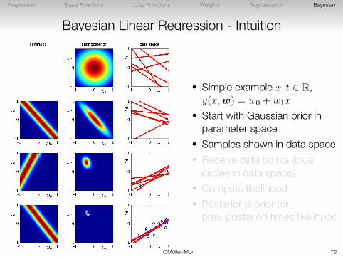
Bayesian Linear Regression - Intuition
• Simple example x, t ∈ R,y(x,w) = w0 + w1x
• Start with Gaussian prior inparameter space
• Samples shown in data space• Receive data points (blue
circles in data space)• Compute likelihood• Posterior is prior (or
prev. posterior) times likelihood
©Möller/Mori 70

Regression Basis Functions Loss Functions Weights Regularization Bayesian
Bayesian Linear Regression - Intuition
• Simple example x, t ∈ R,y(x,w) = w0 + w1x
• Start with Gaussian prior inparameter space
• Samples shown in data space• Receive data points (blue
circles in data space)• Compute likelihood• Posterior is prior (or
prev. posterior) times likelihood
©Möller/Mori 71
Regression Basis Functions Loss Functions Weights Regularization Bayesian
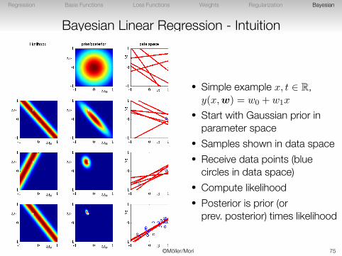
Bayesian Linear Regression - Intuition
• Simple example x, t ∈ R,y(x,w) = w0 + w1x
• Start with Gaussian prior inparameter space
• Samples shown in data space• Receive data points (blue
circles in data space)• Compute likelihood• Posterior is prior (or
prev. posterior) times likelihood
©Möller/Mori 72

Regression Basis Functions Loss Functions Weights Regularization Bayesian
Bayesian Linear Regression - Intuition
• Simple example x, t ∈ R,y(x,w) = w0 + w1x
• Start with Gaussian prior inparameter space
• Samples shown in data space• Receive data points (blue
circles in data space)• Compute likelihood• Posterior is prior (or
prev. posterior) times likelihood
©Möller/Mori 73

Regression Basis Functions Loss Functions Weights Regularization Bayesian
Bayesian Linear Regression - Intuition
• Simple example x, t ∈ R,y(x,w) = w0 + w1x
• Start with Gaussian prior inparameter space
• Samples shown in data space• Receive data points (blue
circles in data space)• Compute likelihood• Posterior is prior (or
prev. posterior) times likelihood
©Möller/Mori 74
Regression Basis Functions Loss Functions Weights Regularization Bayesian
Bayesian Linear Regression - Intuition
• Simple example x, t ∈ R,y(x,w) = w0 + w1x
• Start with Gaussian prior inparameter space
• Samples shown in data space• Receive data points (blue
circles in data space)• Compute likelihood• Posterior is prior (or
prev. posterior) times likelihood
©Möller/Mori 75
Regression Basis Functions Loss Functions Weights Regularization Bayesian
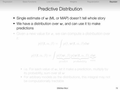
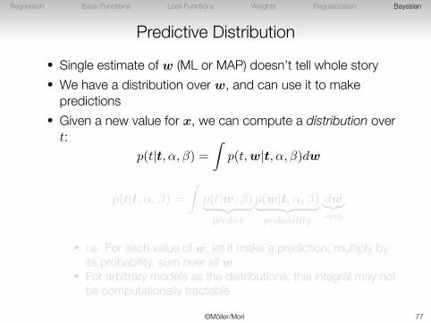
Predictive Distribution• Single estimate of w (ML or MAP) doesn’t tell whole story• We have a distribution over w, and can use it to make
predictions• Given a new value for x, we can compute a distribution overt:
p(t|t, α, β) =∫
p(t,w|t, α, β)dw
p(t|t, α, β) =∫
p(t|w, β)︸ ︷︷ ︸predict
p(w|t, α, β)︸ ︷︷ ︸probability
dw︸︷︷︸sum
• i.e. For each value of w, let it make a prediction, multiply byits probability, sum over all w
• For arbitrary models as the distributions, this integral may notbe computationally tractable
©Möller/Mori 76
Regression Basis Functions Loss Functions Weights Regularization Bayesian
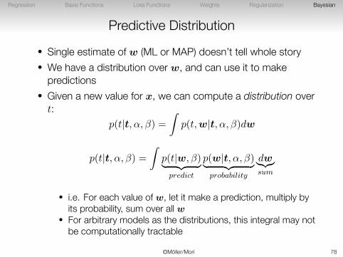
Predictive Distribution• Single estimate of w (ML or MAP) doesn’t tell whole story• We have a distribution over w, and can use it to make
predictions• Given a new value for x, we can compute a distribution overt:
p(t|t, α, β) =∫
p(t,w|t, α, β)dw
p(t|t, α, β) =∫
p(t|w, β)︸ ︷︷ ︸predict
p(w|t, α, β)︸ ︷︷ ︸probability
dw︸︷︷︸sum
• i.e. For each value of w, let it make a prediction, multiply byits probability, sum over all w
• For arbitrary models as the distributions, this integral may notbe computationally tractable
©Möller/Mori 77
Regression Basis Functions Loss Functions Weights Regularization Bayesian
Predictive Distribution• Single estimate of w (ML or MAP) doesn’t tell whole story• We have a distribution over w, and can use it to make
predictions• Given a new value for x, we can compute a distribution overt:
p(t|t, α, β) =∫
p(t,w|t, α, β)dw
p(t|t, α, β) =∫
p(t|w, β)︸ ︷︷ ︸predict
p(w|t, α, β)︸ ︷︷ ︸probability
dw︸︷︷︸sum
• i.e. For each value of w, let it make a prediction, multiply byits probability, sum over all w
• For arbitrary models as the distributions, this integral may notbe computationally tractable
©Möller/Mori 78

Regression Basis Functions Loss Functions Weights Regularization Bayesian
Predictive Distribution
�
�
0 1
−1
0
1
�
�
0 1
−1
0
1
�
�
0 1
−1
0
1
• With the Gaussians we’ve used for these distributions, thepredicitve distribution will also be Gaussian
• (math on convolutions of Gaussians)• Green line is true (unobserved) curve, blue data points, red
line is mean, pink one standard deviation• Uncertainty small around data points• Pink region shrinks with more data
©Möller/Mori 79

Regression Basis Functions Loss Functions Weights Regularization Bayesian
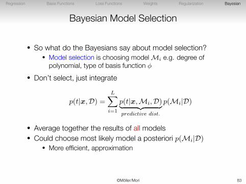
Bayesian Model Selection
• So what do the Bayesians say about model selection?• Model selection is choosing model Mi e.g. degree of
polynomial, type of basis function ϕ
• Don’t select, just integrate
p(t|x,D) =
L∑i=1
p(t|x,Mi,D)︸ ︷︷ ︸predictive dist.
p(Mi|D)
• Average together the results of all models• Could choose most likely model a posteriori p(Mi|D)
• More efficient, approximation
©Möller/Mori 80

Regression Basis Functions Loss Functions Weights Regularization Bayesian
Bayesian Model Selection
• So what do the Bayesians say about model selection?• Model selection is choosing model Mi e.g. degree of
polynomial, type of basis function ϕ
• Don’t select, just integrate
p(t|x,D) =
L∑i=1
p(t|x,Mi,D)︸ ︷︷ ︸predictive dist.
p(Mi|D)
• Average together the results of all models• Could choose most likely model a posteriori p(Mi|D)
• More efficient, approximation
©Möller/Mori 81

Regression Basis Functions Loss Functions Weights Regularization Bayesian
Bayesian Model Selection
• So what do the Bayesians say about model selection?• Model selection is choosing model Mi e.g. degree of
polynomial, type of basis function ϕ
• Don’t select, just integrate
p(t|x,D) =
L∑i=1
p(t|x,Mi,D)︸ ︷︷ ︸predictive dist.
p(Mi|D)
• Average together the results of all models• Could choose most likely model a posteriori p(Mi|D)
• More efficient, approximation
©Möller/Mori 82
Regression Basis Functions Loss Functions Weights Regularization Bayesian
Bayesian Model Selection
• So what do the Bayesians say about model selection?• Model selection is choosing model Mi e.g. degree of
polynomial, type of basis function ϕ
• Don’t select, just integrate
p(t|x,D) =
L∑i=1
p(t|x,Mi,D)︸ ︷︷ ︸predictive dist.
p(Mi|D)
• Average together the results of all models• Could choose most likely model a posteriori p(Mi|D)
• More efficient, approximation
©Möller/Mori 83
Regression Basis Functions Loss Functions Weights Regularization Bayesian
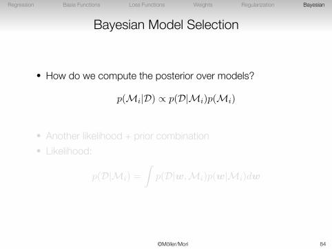
Bayesian Model Selection
• How do we compute the posterior over models?
p(Mi|D) ∝ p(D|Mi)p(Mi)
• Another likelihood + prior combination• Likelihood:
p(D|Mi) =
∫p(D|w,Mi)p(w|Mi)dw
©Möller/Mori 84
Regression Basis Functions Loss Functions Weights Regularization Bayesian
Bayesian Model Selection
• How do we compute the posterior over models?
p(Mi|D) ∝ p(D|Mi)p(Mi)
• Another likelihood + prior combination• Likelihood:
p(D|Mi) =
∫p(D|w,Mi)p(w|Mi)dw
©Möller/Mori 85

Regression Basis Functions Loss Functions Weights Regularization Bayesian
Conclusion
• Readings: Ch. 3.1, 3.1.1-3.1.4, 3.3.1-3.3.2, 3.4• Linear Models for Regression
• Linear combination of (non-linear) basis functions• Fitting parameters of regression model
• Least squares• Maximum likelihood (can be = least squares)
• Controlling over-fitting• Regularization• Bayesian, use prior (can be = regularization)
• Model selection• Cross-validation (use held-out data)• Bayesian (use model evidence, likelihood)
©Möller/Mori 86


