

Manual for the
ArborSonic3D
acoustic tomograph
2019.

1
ArborSonic 3D
User's Manual
v6
January 2, 2019

2
Table of Contents Table of Contents ................................................................................................................................................................ 2 Introduction .......................................................................................................................................................................... 3 Manufacturer information .............................................................................................................................................. 3 Principle of operation ....................................................................................................................................................... 3 Hardware – System parts ................................................................................................................................................ 4 Hardware – Setup ............................................................................................................................................................... 5 Hardware – Handling the Piezo Sensors ................................................................................................................... 6
Maintenance ..................................................................................................................................................................... 6 Fixing ................................................................................................................................................................................... 6 Measurement ................................................................................................................................................................... 6 Removal ............................................................................................................................................................................. 6
Hardware – Amplifier boxes .......................................................................................................................................... 7 Hardware – Battery Box ................................................................................................................................................... 7 Hardware – Bluetooth and serial connection.......................................................................................................... 8
Establishing Bluetooth connection to the Battery Box ................................................................................... 8 Selecting COM port ........................................................................................................................................................ 9
Software – Basics .............................................................................................................................................................. 11 Software – Application Settings .................................................................................................................................. 12 Software – Tree Properties ........................................................................................................................................... 13 Software – Sensor Geometry – Basics ...................................................................................................................... 15 Software – Sensor Geometry – Circular, Elliptical, Rectangular and Irregular ....................................... 16
Circular ............................................................................................................................................................................. 16 Elliptical ........................................................................................................................................................................... 17 Rectangular..................................................................................................................................................................... 17 Irregular ........................................................................................................................................................................... 18
Software – Sensor Geometry – Compass ................................................................................................................. 18 Description ..................................................................................................................................................................... 18 Usage ................................................................................................................................................................................. 18
Software – Time Data ...................................................................................................................................................... 19 Software – Tomograms – Single-layer mode ......................................................................................................... 20 Software – Tomograms – Multi-layer mode .......................................................................................................... 21 Software – Biomechanics ............................................................................................................................................... 22 Software – Image Container ......................................................................................................................................... 24 Software – Generating reports .................................................................................................................................... 25
Report generator – earlier version ....................................................................................................................... 25 Testing and troubleshooting ........................................................................................................................................ 26
Testing before going to the field ............................................................................................................................ 26 Most common troubles and solutions ................................................................................................................. 27
Advice and safety regulations ...................................................................................................................................... 30 Maintenance ........................................................................................................................................................................ 31 Guarantee ............................................................................................................................................................................. 31

3
Introduction
Welcome as a new ArborSonic 3D owner. ArborSonic 3D is designed to detect hidden holes and decay in trees by non-destructive acoustic testing.
Manufacturer information
ArborSonic3D is manufactured by:
Company: Fakopp Enterprise Bt.
EU tax number: HU22207573
Address: Fenyo 26.
City: Agfalva
ZIP: 9423
Country: Hungary
Web: http://www.fakopp.com
E-mail: [email protected]
Phone: +36 99 330 099
Principle of operation
• Several Sensors are placed around the trunk, which are coupled to the tree by steel nails.
• Each Sensor is tapped by a hammer. • The unit measures the travel-time of the sound wave generated by the hammer tap
between each sensor. • If there is a hole, then the sound waves have to pass around the hole and therefore
it requires longer time to reach the opposite sensors.

4
Hardware – System parts
Piezo Sensors
Amplifier Boxes (black)
Battery Box (gray) containing the Bluetooth transmitter
Link Cables
Caliper (optional)
Sensor Remover
Tape measure
Steel and rubber hammers
Case
5
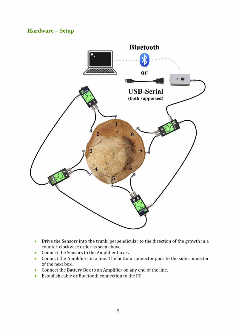
Hardware – Setup
• Drive the Sensors into the trunk, perpendicular to the direction of the growth in a counter-clockwise order as seen above.
• Connect the Sensors to the Amplifier boxes. • Connect the Amplifiers in a line. The bottom connector goes to the side connector
of the next box. • Connect the Battery Box to an Amplifier on any end of the line. • Establish cable or Bluetooth connection to the PC

6
Hardware – Handling the Piezo Sensors
Maintenance
• Always keep the nails, sensor head and the hammer clean, because dirt influences the coupling and time reading.
• The numbers on the sensors are just decoration, you can change them freely, however the numbers on the amplifier boxes are important.
Fixing
• Use the rubber hammer to fix the sensors • The sensors need to go through the bark into the wood • Good coupling between the nail and the wood is essential. The coupling is good if
the sensor head can’t be rotated with 3 stretched fingers. If the sensors can rotate additional hammering is needed to couple the sensors well.
• The sensors need to be in intact wood material, not in decayed material. • The software requires the penetration depth (PD parameter on the Sensor
Geometry tab) of the sensors. This parameter is very important in case of small diameter trees.
• The sensor nails need to point to the center of the trunk; however, this is also not very critical.
• The sensors need to be placed in the same plane. However, this plane doesn’t necessarily have to be horizontal. The plane should be perpendicular to the growth direction. In case of tilting trees, the plane will be tilted as well.
Measurement
• Use the steel hammer for generating the readouts by tapping on the sensor heads. • Remove the tape measure before tapping because it may cause an acoustic short-
circuit. • Always tap on the center of the sensor head in the nail direction. If you accidentally
tapped the side of the sensor, remove the data and tap again. • Tap with uniform strength. Apply more power for large trees. Tapping power is not
very critical, but similar power is recommended. Tap with loose wrist. • Never tap on the cable connection part of the sensor.
Removal
• First disconnect the sensor cable from the amplifier box. Then disconnect the cables. For removing the sensors use the sensor remover tool if possible.
• When removing by hand, first rotate the sensors and then pull. Always pull in nail direction.
• Never pull the cable. • Never use any support to remove the sensors because it may break or bend the
nails.

7
Hardware – Amplifier boxes
• When building up, first fix the sensors,
then the amplifier boxes and finally the
link cables
• Make sure to apply correct connector
orientation when connecting the link
cables. Don't force them.
• Amplifier numbering is essential. Don’t cross the cables
because it will mess up the whole measurement.
• Connect the bottom connector of an amplifier box to the
side connector of the next amplifier box.
• Never move the sensors with attached amplifiers because
it may damage the cable connectors.
• When taking apart, first remove the cables, then the
amplifiers and finally the sensors
Hardware – Battery Box
• Contains the 9V battery and the Bluetooth transmitter.
• Keep the Battery Box turned off while connecting the
Amplifier Boxes.
• The Battery Box can be connected to any amplifier box.
• Make sure to apply correct polarity when changing
battery.
• Any regular or rechargeable 9V battery can be used.
• The LED blinks for 5 seconds after turning on. This is the time required for the Bluetooth
module to warm up.
• If the battery is low, the LED blinks continuously.
• The battery should be well charged.
• It is recommended to turn on the battery box only for the measurement (and keep it turned
off during the rest of the time).
• The battery should be in the proper position.
- +

8
Hardware – Bluetooth and serial connection
• The Battery Box of the device is also responsible for collecting and transmitting data to the
PC (or to an Android smartphone). There are two basic ways to establish connection with
PC: over a Serial-USB cable or over the built-in Bluetooth module (for the smartphone only
Bluetooth connection is possible).
• There are two steps in setting up the connection. The first is to install the USB cable or the
Bluetooth device in Windows. In either way a COM port is assigned to the connection with
a specific number. The second step is to set this number in the software. The software
provides support for both steps.
• The part below deals with setting up the connection over Bluetooth and does not apply if
you choose to use a Serial-USB cable. Please keep in mind that the maximum Bluetooth
range is 30 feet / 10 meters. If you need extended range, longer cable can be used between
the Amplifier Box and the Battery Box.
• For cable connection you may need to install a driver for the serial port itself (the installer
is attached on CD and on pen drive). Then check the ports in the device manager to find out
the proper number of the COM port. This will be used by the device and should be told to
the software. (Note that the number of the COM port depends on the used USB port. If you
connect the cable to another USB port, the COM port’s number will change.)
Establishing Bluetooth connection to the Battery Box
• If the automatic method does not work for any reason, the device needs to be installed
manually in the Control Panel or on the Tray. The final goal of the installation is to set up
and find the COM port number of the device and later set it in the software. (If you are using
an external USB Bluetooth Module, it is recommended to always connect it to the same USB
port.)
• Turn on the Battery Box, start adding a New Bluetooth device in the Control Panel or on
the Tray's Bluetooth Devices function. The device name is ArborSonic 3D.
• The PIN code of the device is 1234.
• The device should be installed by Windows and one or two COM ports should be detected.
Remember the number of the installed COM port. (You can check the Device Manager for
the used COM ports before and after installing the ArborSonic3D device as well, to see
which the new COM ports are belonging to the ArborSonic3D.)
• Start the software.
9
Selecting COM port
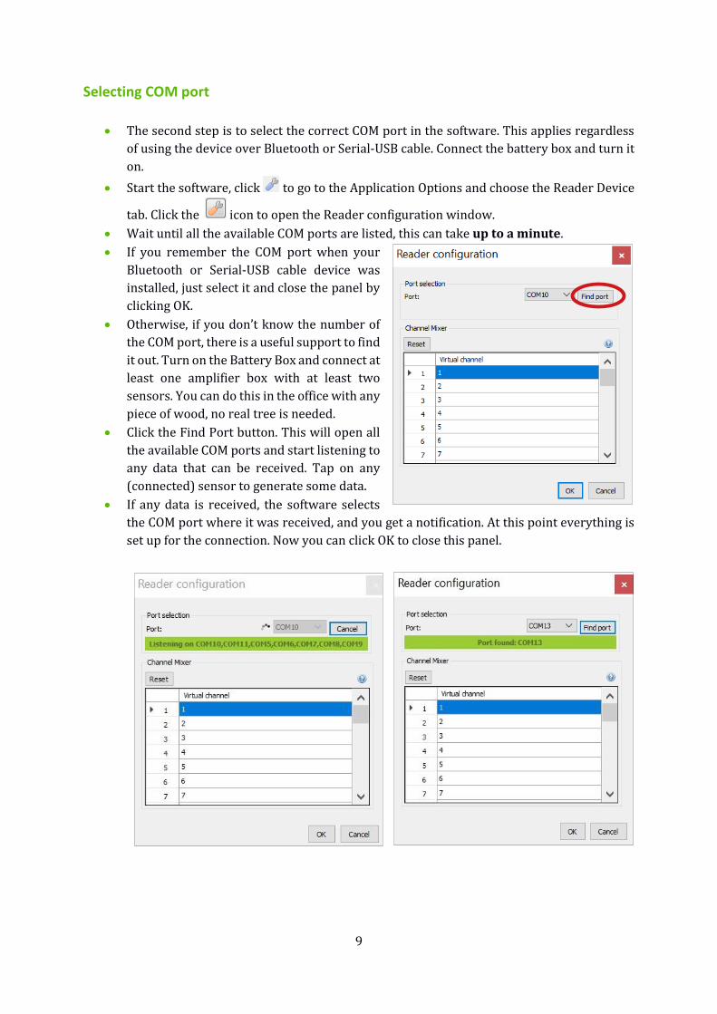
• The second step is to select the correct COM port in the software. This applies regardless
of using the device over Bluetooth or Serial-USB cable. Connect the battery box and turn it
on.
• Start the software, click to go to the Application Options and choose the Reader Device
tab. Click the icon to open the Reader configuration window.
• Wait until all the available COM ports are listed, this can take up to a minute.
• If you remember the COM port when your
Bluetooth or Serial-USB cable device was
installed, just select it and close the panel by
clicking OK.
• Otherwise, if you don’t know the number of
the COM port, there is a useful support to find
it out. Turn on the Battery Box and connect at
least one amplifier box with at least two
sensors. You can do this in the office with any
piece of wood, no real tree is needed.
• Click the Find Port button. This will open all
the available COM ports and start listening to
any data that can be received. Tap on any
(connected) sensor to generate some data.
• If any data is received, the software selects
the COM port where it was received, and you get a notification. At this point everything is
set up for the connection. Now you can click OK to close this panel.

10
• Other possibility is to use the Port Diagnostics on the same panel (on the Reader device tab
of the Application Options). Click to this button.
o It opens the SerialPort
diagnostics window. The
program automatically looks
for the used COM ports. (It can
take a few minutes.)
o Generate data by tapping the
connected sensors.
o The COM ports are listed on
the top and if any data could be
received it is shown in the
window. The raw data can be
saved if it is needed.
o By clicking Close the window
will close. If the COM set in the program is not same which sent the last data, the
SerialPort diagnostics the program will ask if the COM port can be changed. Push
Yes if the last received data was from the ArborSonic device.
o The information sent by ArborSonic starts with IN (referring to incoming data),
followed by two numbers which refers to the Amplifier Box which sent the data (00
is for the Amplifier Box with 1st and 2nd sensors, 01 is for the Amplifier Box with 3rd
and 4th sensors, 02 is for the Amplifier Box with the 5th and 6th sensors and so on).
The following 2 four-digit numbers are the time data detected by the proper
sensors.
For example a line can be IN 03 0205 0311 which means the Amplifier Box with the
7th and 8th sensors sent the data 205µs from the 7th sensor and 311µs from the 8th
sensor.
• To check if everything is fine, restart the program, create a dummy layer with some dummy
geometry parameters (the simplest is to choose a circle), and go to the Time Data page.
(You may have to push „Start”.) If the connection is set up successfully, a green “Reading
device (COM_)” message should appear. Start tapping the sensors and you should see rows
of numbers arriving in the table below.

11
Software – Basics
• The latest version of the software can be downloaded at http://www.fakopp.com.
• The software can be installed to any PC with Windows 7 or higher.
• The software includes the following:
o Selecting parameters of the tree (species, ...)
o Registering the geometry of the sensors
o Collecting the time data from ArborSonic 3D over Bluetooth or via USB cable
o Computing the internal cross-sectional tomogram
o Performing safety factor calculations
o Generating a report file for customers
o Saving and opening previous projects
• The steps of a measurement are:
1. Choosing the measurement Layer on the trunk.
2. Starting the software and selecting the tree species.
3. Placing the sensors (to the proper positions calculated by the software when using
circle, elliptic or rectangular geometry) and registering the sensor geometry
manually or with the Bluetooth Caliper (in case of irregular geometry).
4. Collecting time data by tapping on each sensor.
5. If measurements at several layers are required, choose the next layer and repeat
the previous two steps.
6. Evaluating the cross-sectional maps, tomograms.
7. Performing stability computations.
8. Saving and exporting data to the report file which can be printed later.

12
Software – Application Settings
• To access the application settings, click .
This panel is divided into several tabs for
changing different settings of the software.
• On the User Connection tab, you can leave
your contact details which will only be used
in case of software problems, so we can get
in touch with you and help with the solution.
In case of a software problem an error report
is sent to us in email. You can select whether
this email should be sent automatically or
not and whether it should contain your
contact information and the current project.
• On the User Interface tab, you can select the
software language and the measurement
system which can be Metric or American
Standard.
• The Reader Device tab can be used to set up
and configure the Bluetooth settings with the
ArborSonic 3D device. The button Start
starts an automatic detection which can be
used if a new device should be installed. The
process is different according to the
operation system and the used computer.
The ArborSonic3D device should be
connected and a signal is needed.
• The “Reader Configuration” button
opens the same window as the same button on the Time Data page of the software. This
window is responsible for selecting the COM port which is explained in the “Selecting COM
port” section. The channel mixer tool lets you assign different numbering for the physical
channel numbers as printed on the Amplifier Boxes. This is useful if you lose one of the
boxes, let’s say 5-6, but still want to perform measurements with 8 sensors using boxes 1-
2, 3-4, 7-8, 9-10. (Detailed in chapter Testing and Troubleshooting.)
• Port diagnostics is a tool that is useful for monitoring the raw data received from the
device. Actually, it is a simple telnet application. It opens all the ports and listens to any
data that is received. Using the Save button the data can be saved to an external file.
• On the Bluetooth Caliper page, you can select the COM port of the Bluetooth Caliper.
• On the Updater page you can disable or enable automatic software updates over the
internet. By default, this feature is turned on, so you will receive updates automatically
when starting the software.
• On the Advanced tab Zero limit is the number under which a measured time value is
considered as zero. The default and recommended setting is 0 which in fact turns this
function off.
13
• Auto filter limit is the difference limit in time which if reached results the measured time
row to be filtered out. The default setting is 20.
• Min. good row count is the number of required good time measurements from each sensor.
The default setting is 3.
• Minimal and maximal T0 are internal time correction limit parameters which are out of the
scope of this manual. The default settings are 20 and 35. You have to change these values if
you are using long (e.g. 12 cm / 4.7 inches) nails. In this case T0 min should be 45 while T0
max should be set to 60.
• Velocity scale controls the scale (height) of the 3D map in the z axis.
• Rel Time Error Threshold controls the level above which the values in the time matrix on
the Time Data panel are shown as red, if the relative error exceeds this limit. The default is
5%.
• Minimal Line Velocity is an internal minimum value for any measured line velocity, default
is 500 meter/sec.
• Software rendering should be used if you experience problems with the tomogram images.
The program must be restarted if this setting is changed.
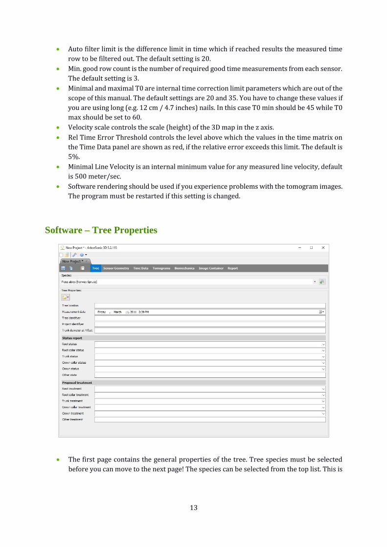
Software – Tree Properties
• The first page contains the general properties of the tree. Tree species must be selected
before you can move to the next page! The species can be selected from the top list. This is

14
a quick list which contains maximum 20 of the recently used species. To select a species
which is not in this list, click the button. A
new window pops up where you can navigate
in the taxonomical list of tree species. This list
contains above 3000 species. To speed up the
search process, you don’t need to click through
the whole list to find a species, but you can
simply start typing the English or Latin name
of the species. To jump to the next candidate,
click or hit the enter button. After
selecting the desired species, click OK to close
this window.
• The rest of this page contains various fields for
describing different properties of the tree. The
software comes with a default tree property
template, but it is possible to create custom templates which may be used to register
different properties. All this will go into the report that is generated by the software, so a
well-designed template can save you a lot of time. Of course, changing this template is
optional and you can start working with the default template.
• Click the button to open the tree properties menu. Select Open for opening another
template, New for creating a new one, Edit to modify an existing one or Remove to delete.
The default template that comes with the software can’t be deleted.
• When selecting New or Edit, the template editor
window pops up. The left side of this window
shows the preview of the template while the right
side can be used to add, remove and modify distinct
fields in the template.
• By clicking the button a new field can be added
to the template. The type of the new field and its
position relative to the current selection must be
selected. After clicking OK the properties of this
field can be set. For example, each field type has a Name property which is the display name
of this field.
• The buttons can be used to change the
relative position of the selected field and the
button can be used to remove it. The
buttons can be used to save the modifications to the
template or to save it under a new name. After this
the template is ready to be opened for use.
15
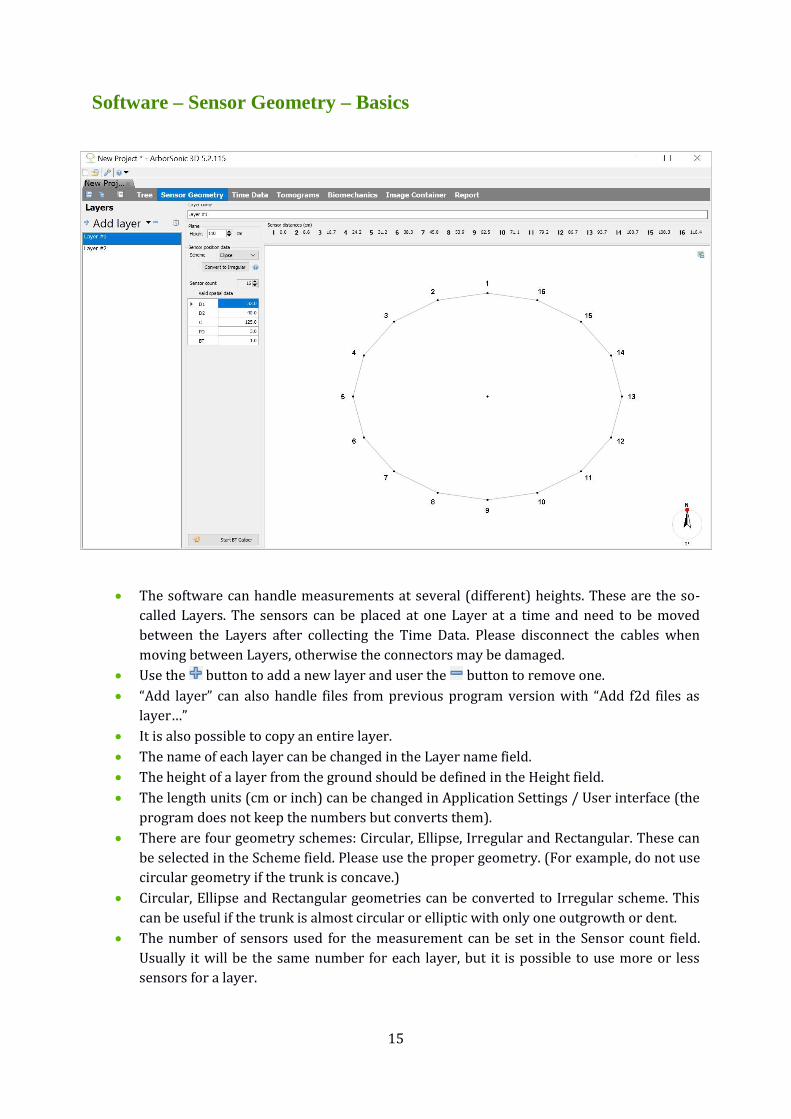
Software – Sensor Geometry – Basics
• The software can handle measurements at several (different) heights. These are the so-
called Layers. The sensors can be placed at one Layer at a time and need to be moved
between the Layers after collecting the Time Data. Please disconnect the cables when
moving between Layers, otherwise the connectors may be damaged.
• Use the button to add a new layer and user the button to remove one.
• “Add layer” can also handle files from previous program version with “Add f2d files as
layer…”
• It is also possible to copy an entire layer.
• The name of each layer can be changed in the Layer name field.
• The height of a layer from the ground should be defined in the Height field.
• The length units (cm or inch) can be changed in Application Settings / User interface (the
program does not keep the numbers but converts them).
• There are four geometry schemes: Circular, Ellipse, Irregular and Rectangular. These can
be selected in the Scheme field. Please use the proper geometry. (For example, do not use
circular geometry if the trunk is concave.)
• Circular, Ellipse and Rectangular geometries can be converted to Irregular scheme. This
can be useful if the trunk is almost circular or elliptic with only one outgrowth or dent.
• The number of sensors used for the measurement can be set in the Sensor count field.
Usually it will be the same number for each layer, but it is possible to use more or less
sensors for a layer.

16
• PD is a parameter required for all three schemes. It is the penetration depth of the nail tip
from the bark surface. It is not a very critical parameter, especially in case of large trees.
But it is important in case of smaller trees.
• BT is another parameter required for all schemes and denotes the Bark Thickness. This
parameter is not very critical in case of normal sized trees, but it should be set carefully for
small trees.
• For measurements physical penetration depth should always be more than the bark
thickness, the nail should go through the bark.
• In Circular, Ellipse and Rectangular the software tells you where to put the sensors.
• In Irregular first you place the sensors and then you tell the software where they are.
• Different layers can have different schemes.
• Sensors need to be placed in a counter-clockwise order when seen from above. Therefore,
previous sensors need to be on the left side while next sensors on the right side.
Software – Sensor Geometry – Circular, Elliptical, Rectangular and
Irregular
Circular
• Use this scheme if the trunk is circular.
• Place sensor no. 1 anywhere and use it as a support to hold
the tape around the trunk. (The north direction is included in
the program. The layer can be rotated by the red/green dot
on the top of the compass (the arrow in corner) indicating
north direction. It can become important if the sensors are
not at the same directions in the different layers. Detailed in
chapter Software – Sensor Geometry – Compass.)
• Measure the circumference with the tape and type it into C.
• Place the other sensors around the trunk at the positions
displayed:
• Provide the estimated penetration depth of the sensor nail tip from the bark surface as the
PD parameter. (The nails’ lengths are usually 6 cm.)
• Provide the estimated bark thickness as the BT parameter.
• By pressing the “Convert to irregular” button, the scheme will be converted to Irregular
(see below) which might be useful when the tree is almost circular, but the positions of one
or two sensors need to be adjusted.

17
Elliptical
• Use this scheme if the trunk is elliptical.
• Place sensor no. 1 at the end of the larger diameter and use it as a support to hold the tape
around the trunk.
• Measure the circumference with the tape and type it in parameter C.
• Measure the larger diameter with a caliper and type it in D1. Measure the smaller diameter
and type it in D2.
• Place the other sensors around the trunk at the positions displayed:
• Direction, PD and BT can be adjusted the same as detailed above for circular geometry.
• By pressing the “Convert to irregular” button, the scheme will be converted to Irregular
(see below) which might be useful when the tree is almost elliptical, but the positions of
one or two sensors need to be adjusted.
Rectangular
• Use this scheme if you are investigating rectangular wood.
• A is the width of the rectangle and B is its depth.
• ASC and BSC are the number of sensors on the A and B side. 2*(ASC+BSC) must equal the
total number of sensors, otherwise you get a sensor count mismatch.
• LeftPad, RightPad, TopPad, BottomPad are the spacings between the corner and the first
sensor from the given direction. These must be smaller than A or B.
• By pressing the “Convert to irregular” button, the scheme will be converted to Irregular
(see below) which might be useful when the shape is almost rectangular, but the positions
of one or two sensors need to be adjusted.
• Direction, PD and BT can be adjusted the same as detailed above for circular geometry.

18
Irregular
• Use this scheme if the trunk shape is irregular.
• Place the sensors around the trunk in counter-clockwise order.
• Make sure that the sensors are in one plane. The tape measure can be used for this.
• After placing the sensors use the caliper to measure distances between sensor pairs. For
example, distance between sensor no. 1 and no. 2 needs to be entered in the field .
• The Bluetooth caliper can be used to transmit the data automatically. Just start the caliper
and measure the appropriate distances.
• Direction, PD and BT can be adjusted the same as detailed above for circular geometry.
• The other shapes can be converted into irregular. Change the distances of the sensor(s)
which is not fitting the previously used shape.
Software – Sensor Geometry – Compass
Description
• The compass is the graphic in the lower right corner.
• Using the compass is optional.
• It can be used to specify a direction of interest, relative to north. (E.g. it
can be used to specify the positions of the trees, of the sensors.)
• It rotates all views of the selected layer (except the multilayer view).
(Therefore it can be used it to rotate the layer according to your viewing angle of the tree.)
• The specified angle is saved, when you save your project.
Usage
• The angle needs to be set separately for each layer.
• The angle is represented by a dot on the circle. The exact value is
displayed at the bottom, in degrees.
• The angle can only be changed on the Sensor Geometry page. This is
indicated by its red color.
• When on the Sensor Geometry page, hover your mouse over the dot, and press down the
left mouse button while you move it to its new place. While this is done, the color of the dot
will be green.
• On all other pages the dot will be colored black, to indicate that it cannot be edited.
• On Sensor Geometry tab the default position of the first sensor on the top (facing to north).
You may measure different layers with the sensors facing to different directions and rotate
them to proper positions. You can check the relative positions of the layer in the multi-layer
mode.
19
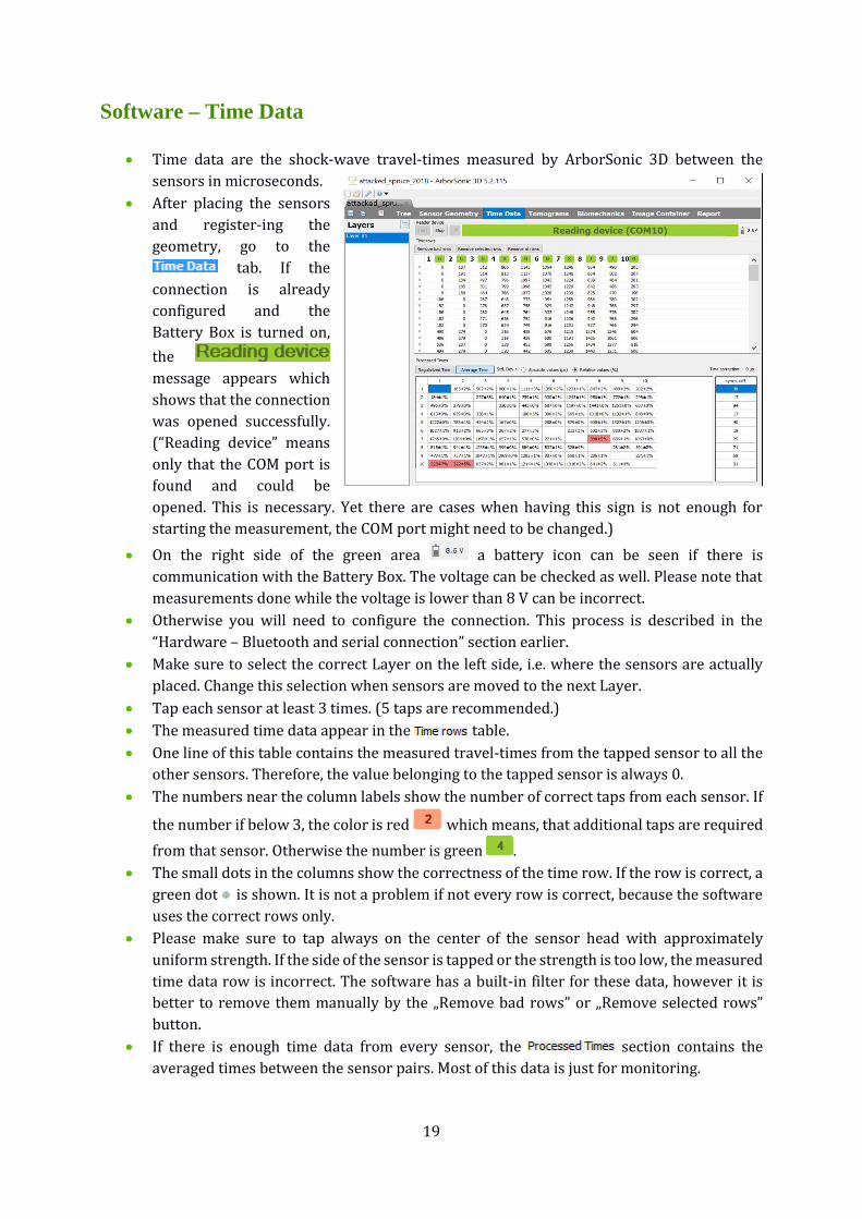
Software – Time Data
• Time data are the shock-wave travel-times measured by ArborSonic 3D between the
sensors in microseconds.
• After placing the sensors
and register-ing the
geometry, go to the
tab. If the
connection is already
configured and the
Battery Box is turned on,
the
message appears which
shows that the connection
was opened successfully.
(“Reading device” means
only that the COM port is
found and could be
opened. This is necessary. Yet there are cases when having this sign is not enough for
starting the measurement, the COM port might need to be changed.)
• On the right side of the green area a battery icon can be seen if there is
communication with the Battery Box. The voltage can be checked as well. Please note that
measurements done while the voltage is lower than 8 V can be incorrect.
• Otherwise you will need to configure the connection. This process is described in the
“Hardware – Bluetooth and serial connection” section earlier.
• Make sure to select the correct Layer on the left side, i.e. where the sensors are actually
placed. Change this selection when sensors are moved to the next Layer.
• Tap each sensor at least 3 times. (5 taps are recommended.)
• The measured time data appear in the table.
• One line of this table contains the measured travel-times from the tapped sensor to all the
other sensors. Therefore, the value belonging to the tapped sensor is always 0.
• The numbers near the column labels show the number of correct taps from each sensor. If
the number if below 3, the color is red which means, that additional taps are required
from that sensor. Otherwise the number is green .
• The small dots in the columns show the correctness of the time row. If the row is correct, a
green dot is shown. It is not a problem if not every row is correct, because the software
uses the correct rows only.
• Please make sure to tap always on the center of the sensor head with approximately
uniform strength. If the side of the sensor is tapped or the strength is too low, the measured
time data row is incorrect. The software has a built-in filter for these data, however it is
better to remove them manually by the „Remove bad rows” or „Remove selected rows”
button.
• If there is enough time data from every sensor, the section contains the
averaged times between the sensor pairs. Most of this data is just for monitoring.
20
• The standard deviation of the average of the times measured between each sensor pair is
shown after the signs. The standard deviations can be displayed in microseconds or in
relative values. If the relative error is above 5%, then the corresponding cell is shown as
red and it is advised to check the table, remove rows far from the average or simply
collect some more data for the affected sensors.
• When tapping on each sensor, the time between each sensor pair is measured in two
different ways: when one of the sensors is tapped and the other is the receiver and in the
reverse direction. The table contains the average differences between the times
measured in both directions for all sensors. This table is a handy tool for finding bad
sensors: if the value for one sensor is unusually high (above 100), then the sensor may be
in a bad position (the tip is in decayed wood or in a hollow), broke or the tape measure was
not removed from the trunk.
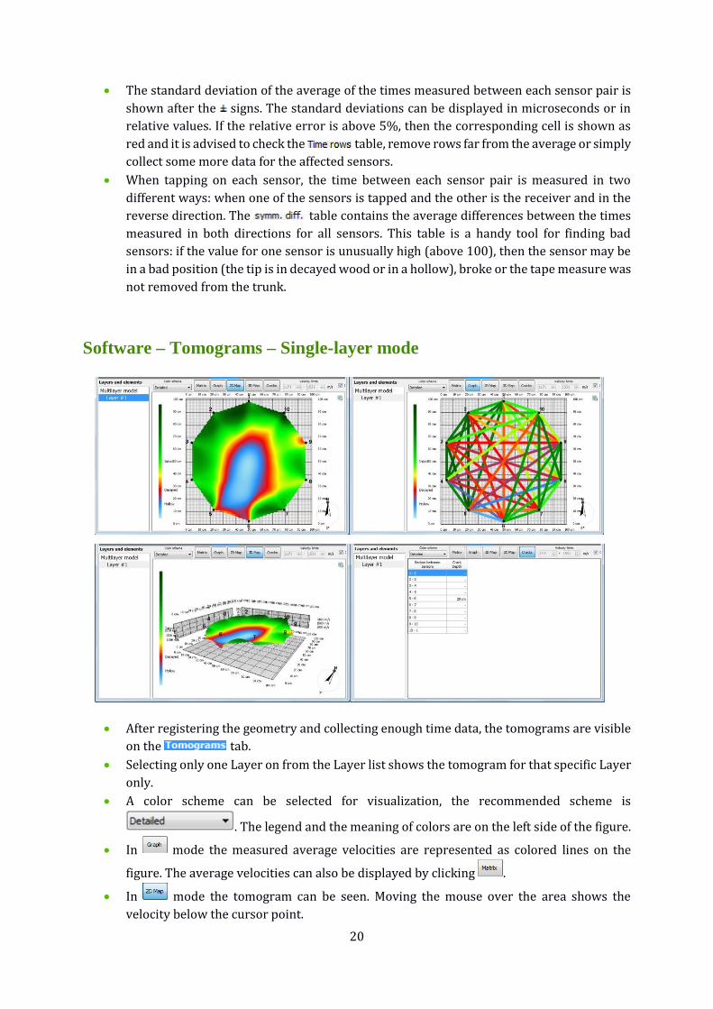
Software – Tomograms – Single-layer mode
• After registering the geometry and collecting enough time data, the tomograms are visible
on the tab.
• Selecting only one Layer on from the Layer list shows the tomogram for that specific Layer
only.
• A color scheme can be selected for visualization, the recommended scheme is
. The legend and the meaning of colors are on the left side of the figure.
• In mode the measured average velocities are represented as colored lines on the
figure. The average velocities can also be displayed by clicking .
• In mode the tomogram can be seen. Moving the mouse over the area shows the
velocity below the cursor point.
21
• In mode the tomogram is represented as a 3-dimensional surface.
• The Cracks mode tries to estimate crack depths which start from the surface. The estimated
crack depth between each sensor is displayed in the list. However, this tool does not detect
internal cracks.
• By checking the checkbox, the velocity limits which set the colors are
calculated automatically and this is the recommended setting. However, by un-checking
this checkbox allows for manual modification of the velocity limits.
• Use the icon on the top right corner to save a view to the Image Container.
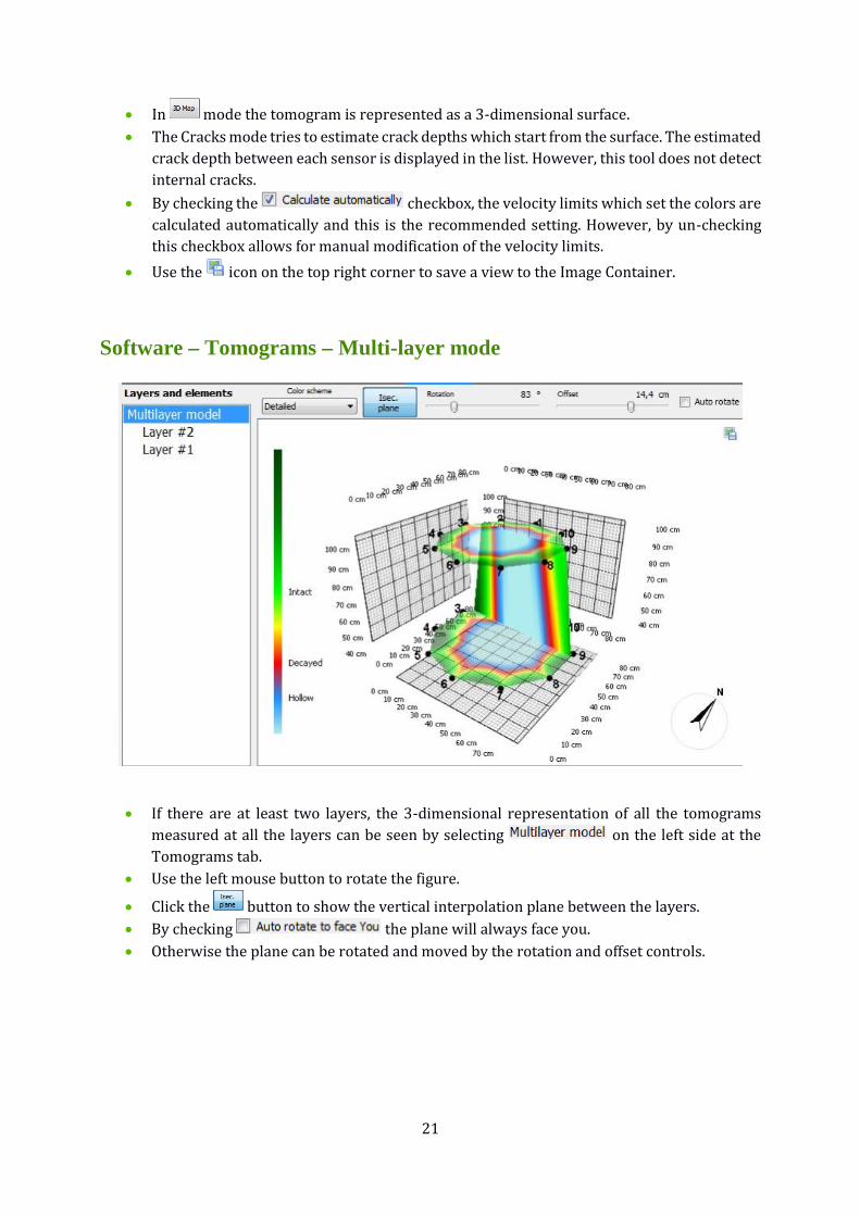
Software – Tomograms – Multi-layer mode
• If there are at least two layers, the 3-dimensional representation of all the tomograms
measured at all the layers can be seen by selecting on the left side at the
Tomograms tab.
• Use the left mouse button to rotate the figure.
• Click the button to show the vertical interpolation plane between the layers.
• By checking the plane will always face you.
• Otherwise the plane can be rotated and moved by the rotation and offset controls.

22
Software – Biomechanics
• The Biomechanics page allows you to evaluate the Safety Factor of the tree trunk using the
obtained cross-sectional tomograms at the specified wind load.
• The process gives an estimate
for the trunk safety. Please
note that only the tomograms
at the measurement Layers
are used, therefore the
software is not aware of any
parts outside the
measurement region.
• It is possible to measure
different parameters of the
tree from a photo. Click the
button on the Image
Container section and load a photo of the tree. It is recommended to take the photo from a
distance of at least the height of the tree to avoid distortions. If the tree has substantial
inclination, then it is recommended to take the photo from a direction where this
inclination can be seen. After loading and selecting the photo you can use the button
to collapse the image container to gain more space on the screen. Please note that you can
enter all the necessary parameters without a photo as well, marking dimensions on a photo
is an option to make the process more convenient.
• Use the button to mark the shape of the crown. Click once for each point. Closing the
curve and finishing marking can be achieved by clicking the same button again.
• The reference length can be marked with the button. Two clicks place a blue line with
a “???” text on the line. Click the text to enter the reference length (in meters if using metric
system) of this line. This line should mark a person or some reference object on the photo,
placed at the distance of the tree.
• The button can be used to measure the degree of tilting (lean) of the trunk. It can place
a yellow line of two-line segments defined by three points. The middle point marked by a
square should be placed at the bottom of the trunk, one of the endpoints marked by a circle
should point in the direction of the trunk and the other one should point to the horizontal
direction. Click the same button again to finish marking. This marks the tilt angle of the
tree. (The points can be moved by mouse. If it is impossible to predict the actual tilting from
the photo you can modify the data manually.) 0° means tilting towards east.
• On the left the first parameter is the Crown Area. This can be entered either from the photo
as described earlier, or manually, or using the crown area calculator by clicking . This
tool requires the width, height of the crown and a shape factor. The calculated area is
simply width times height times factor. Predefined factors can be selected by choosing the
assumed crown shape. (Using a custom factor is also possible.)
• The distances from the trunk bottom to the crown center and crown top need to be
provided. These parameters can also be taken from the photo if everything is marked
appropriately.
23
• The next parameter is the tilt angle which can also be taken from the photo. 90 degrees
mean a completely vertical trunk.
• Tilt direction is not taken from the photo and always needs to be provided manually. The
value is the relative degree to east 0 degree means tilting toward east.
• Wind velocity must be set to the highest expected wind speed. Which is usually 33m/s or
75 mph but can be even higher like 40 m/s in coasts, mountain areas and so.
• Drag factor is the drag coefficient of the crown, taken from the tree species database.
• Yield strength is the yield strength of the trunk wood, also taken from the species database.
• The table lists all the layers. The first column is the name of the layer, the second column is
the layer height as provided on the Geometry page. The third column is the Decayed area
regarding the cross-sectional area in the given height. It is the percentage of the decayed
region of the selected layer compared to the total layer area. Safety Factor is in the fourth
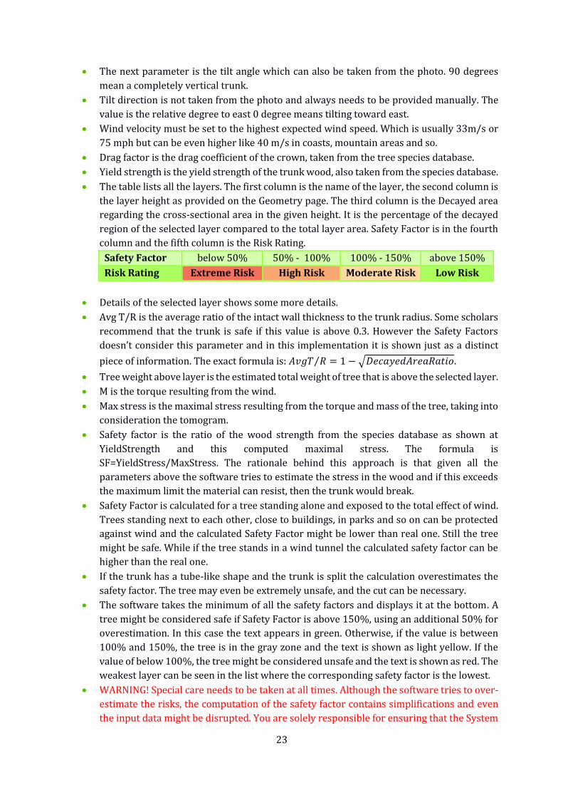
column and the fifth column is the Risk Rating.
Safety Factor below 50% 50% - 100% 100% - 150% above 150%
Risk Rating Extreme Risk High Risk Moderate Risk Low Risk
• Details of the selected layer shows some more details.
• Avg T/R is the average ratio of the intact wall thickness to the trunk radius. Some scholars
recommend that the trunk is safe if this value is above 0.3. However the Safety Factors
doesn’t consider this parameter and in this implementation it is shown just as a distinct
piece of information. The exact formula is: 𝐴𝑣𝑔𝑇 𝑅⁄ = 1 − √𝐷𝑒𝑐𝑎𝑦𝑒𝑑𝐴𝑟𝑒𝑎𝑅𝑎𝑡𝑖𝑜.
• Tree weight above layer is the estimated total weight of tree that is above the selected layer.
• M is the torque resulting from the wind.
• Max stress is the maximal stress resulting from the torque and mass of the tree, taking into
consideration the tomogram.
• Safety factor is the ratio of the wood strength from the species database as shown at
YieldStrength and this computed maximal stress. The formula is
SF=YieldStress/MaxStress. The rationale behind this approach is that given all the
parameters above the software tries to estimate the stress in the wood and if this exceeds
the maximum limit the material can resist, then the trunk would break.
• Safety Factor is calculated for a tree standing alone and exposed to the total effect of wind.
Trees standing next to each other, close to buildings, in parks and so on can be protected
against wind and the calculated Safety Factor might be lower than real one. Still the tree
might be safe. While if the tree stands in a wind tunnel the calculated safety factor can be
higher than the real one.
• If the trunk has a tube-like shape and the trunk is split the calculation overestimates the
safety factor. The tree may even be extremely unsafe, and the cut can be necessary.
• The software takes the minimum of all the safety factors and displays it at the bottom. A
tree might be considered safe if Safety Factor is above 150%, using an additional 50% for
overestimation. In this case the text appears in green. Otherwise, if the value is between
100% and 150%, the tree is in the gray zone and the text is shown as light yellow. If the
value of below 100%, the tree might be considered unsafe and the text is shown as red. The
weakest layer can be seen in the list where the corresponding safety factor is the lowest.
• WARNING! Special care needs to be taken at all times. Although the software tries to over-
estimate the risks, the computation of the safety factor contains simplifications and even
the input data might be disrupted. You are solely responsible for ensuring that the System

24
is appropriate for the use you put it to, and you understand that is only one part of what is
needed to assess the health of trees and similar green assets. Please understand that the
System is just one tool to be used, along with your experience and training in assessing
these living organisms, that the System cannot be relied upon as the sole source of
evaluations, and that all hardware and software is subject to failure or misuse.
Software – Image Container
• The image container is the place where the images are stored. This is to where you can
export your tomograms from any view in the software with the button and these will
be exported later into the generated report. This is the same container as the one you can
access from the Biomechanics page.
• You can open an external image with the button and export an image from this
container to an external file with the button. The button can be used to remove an
image from the container.
• Use the , buttons (or the slider between them) to change what size the images are
shown at. This does not change however the actual size of the images.
• Clicking the title of an image or using button allows you to change it.
25
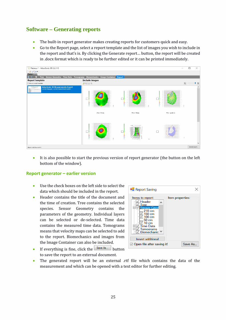
Software – Generating reports
• The built-in report generator makes creating reports for customers quick and easy.
• Go to the Report page, select a report template and the list of images you wish to include in
the report and that’s is. By clicking the Generate report… button, the report will be created
in .docx format which is ready to be further edited or it can be printed immediately.
• It is also possible to start the previous version of report generator (the button on the left
bottom of the window).
Report generator – earlier version
• Use the check boxes on the left side to select the
data which should be included in the report.
• Header contains the title of the document and
the time of creation. Tree contains the selected
species. Sensor Geometry contains the
parameters of the geometry. Individual layers
can be selected or de-selected. Time data
contains the measured time data. Tomograms
means that velocity maps can be selected to add
to the report. Biomechanics and images from
the Image Container can also be included.
• If everything is fine, click the button
to save the report to an external document.
• The generated report will be an external .rtf file which contains the data of the
measurement and which can be opened with a text editor for further editing.
26
Testing and troubleshooting
This chapter describes how to test your equipment. Please read this chapter carefully if you did
not use your device for more than 3 months and you are planning to go to the field.
The most common troubles, errors and misuses are also described with the most probable
solutions.
Testing before going to the field
• Please check if the battery is well charged. The Bluetooth connection needs much charge.
(Sometimes even new and unused batteries don’t have enough charge.)
• Hammer two sensors to any piece of wood if it is possible. No tree is needed only a piece
of wood.
• Connect the two sensors to one Amplifier Box and connect it to the Battery Box.
• Start the program on your computer and turn on the Battery Box.
• Check the COM port connection (as in the chapter Hardware – Bluetooth and serial
connections).
• Go to the Time Data tab of the program and hit one of the sensors. If time data is arriving,
these parts of the device are ready to work.
• If you cannot find any piece of wood, you can gently tap the sensor nails to each other
and see if you get any new row on the Time Data tab.
• You may check all the Amplifier Boxes and sensors.
• The best is to have a tree nearby (in a garden or park) or a testing log and make a whole
measurement similar to measurements done on field.

27
Most common troubles and solutions
Trouble Solution
Battery Box is not turning on. Check the battery, charge or replace it with a new
and/or charged one. Switch on and off the unit
several times. (It is recommended to turn off the
battery after each measurement and turn it on only
for the duration of the measurement.)
There is no signal from one
sensor or sensor pair.
Check the cables and their orientations.
There is no signal after hitting
any sensor.
Check the Battery Box. Check the serial cable if you
are using cable connection.
If you are using Bluetooth check if the Battery Box
is shielded by the tree. If the Battery Box cannot see
the computer / smartphone relocate the computer,
the phone or the Battery Box. (You can connect the
Battery Box to any Amplifier Box, just be sure that
all other Amplifier Boxes are connected to their
neighbors.)
Check if you are using the proper COM port.
If you have used cable connection try it via
Bluetooth. If you have used Bluetooth try it with
cable connection.
There is the green “Reading
device (COM__)” on the Time
Data tab, but there is no data
coming from any of the sensors.
Please check if you are connected to right COM
port. (See sub-chapter “Selecting COM port” for
more information.)
Time row without ‘zero’.
It is just a bad measurement row. You can delete it
by Remove bad rows or let it there (the calculation
will not use these data). You may have to hit some
sensors again.
28
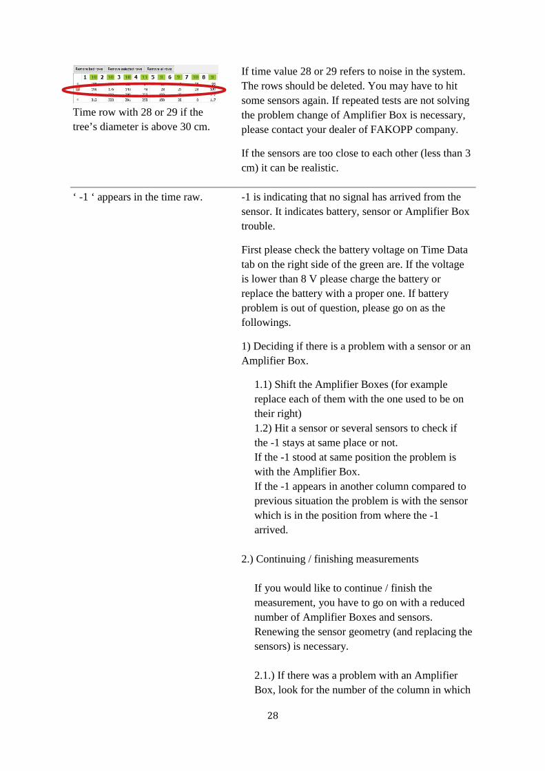
Time row with 28 or 29 if the
tree’s diameter is above 30 cm.
If time value 28 or 29 refers to noise in the system.
The rows should be deleted. You may have to hit
some sensors again. If repeated tests are not solving
the problem change of Amplifier Box is necessary,
please contact your dealer of FAKOPP company.
If the sensors are too close to each other (less than 3
cm) it can be realistic.
‘ -1 ‘ appears in the time raw.
-1 is indicating that no signal has arrived from the
sensor. It indicates battery, sensor or Amplifier Box
trouble.
First please check the battery voltage on Time Data
tab on the right side of the green are. If the voltage
is lower than 8 V please charge the battery or
replace the battery with a proper one. If battery
problem is out of question, please go on as the
followings.
1) Deciding if there is a problem with a sensor or an
Amplifier Box.
1.1) Shift the Amplifier Boxes (for example
replace each of them with the one used to be on
their right)
1.2) Hit a sensor or several sensors to check if
the -1 stays at same place or not.
If the -1 stood at same position the problem is
with the Amplifier Box.
If the -1 appears in another column compared to
previous situation the problem is with the sensor
which is in the position from where the -1
arrived.
2.) Continuing / finishing measurements
If you would like to continue / finish the
measurement, you have to go on with a reduced
number of Amplifier Boxes and sensors.
Renewing the sensor geometry (and replacing the
sensors) is necessary.
2.1.) If there was a problem with an Amplifier
Box, look for the number of the column in which

29
the -1 appeared. Look for the Amplifier Box with
that number (all Amplifier Boxes have 2
numbers on them referring the 2 sensors they are
connected to). Disconnect the wrong Amplifier
Box. Open Application Options go to Reader
Device tab and click onto for Reader
configurations. Here at Channel Mixer you can
change the Virtual channels (the channels known
by the program) of the physical ones. For
example, if the Amplifier Box 3-4 is wrong set 1
to 1, 2 to 2, 3 to for example 31, 4 to for example
32 (higher than the sensor count you will use), 5
to 3, 6 to 4 and so.
When you set the acting Amplifier Boxes be very
careful about their positions because the
numbering is shifted.
2.2) If there was a problem with a sensor,
disconnect and remove the last Amplifier Box. In
this way you have extra 2 sensors. Replace the
bad sensor with a good one. (The sensors are
identical, numbers are decorations only.)
3) Long-term solution
3.1.) If there was a problem with an Amplifier
Box, please contact Fakopp company or our
dealer in your area.
3.2) If there was a problem with a sensor you
may replace the BNC connection on the end. It
helps in most of the cases. Otherwise please
contact Fakopp company or our dealer in your
area.

30
Advice and safety regulations
Be aware, the sensors' tips are pointed.
Clean the device after measurement. Sterilize the sensors if there is a risk of infection.
Check the batteries before going to the field.
Do not break the cables, sensors, boxes, any part of the device.
Take care of your fingers, toes,… while placing the sensors onto the tree and during measuring,
hitting the sensors with the hammers.
Fix the sensors with the rubber hammer and generate sound signals for measurement with the
steel hammer.
Do not start acoustic and resistivity measurements at the same time on the same tree.
If you expect to measure trees with elliptic or irregular trunk shape, it is recommended to bring
a caliper as well.
Do not use the acoustic tomograph if the temperature is below 0 °C / 32 °F or more than
40 °C / 100 °F.
Do not use the device in heavy storms, raining or in foggy conditions.
Bringing a folding table with yourself to the measurement is recommended for holding the
computer.
This device is for measuring living trees and some wooden structures. Do not use it for any other
purpose.
Do not open the amplifier boxes or the sensors. If there is a problem with the device, please
contact us. Opening the parts cancels all guarantee.
The device includes sensitive parts as well, do not drop it, step onto it, put it under water.
(Sensors specialized for underwater measurements are available.)
Always save the data after the measurement.

31
Maintenance
Keep the device in a dry place in room temperature.
If you have to clean it, please use a lightly wet towel.
If resin got to the sensors you can clean them with benzine. Take care of the handling of the
chemical.
If any of the parts are broken please contact us.
It is recommended to switch off the device after measurement.
Do not break the cables and keep them coiled up to avoid tangle.
Guarantee
The guarantee lasts for one year from the arrival of the device.


