
Mathematical Economics:Lecture 14
Yu Ren
WISE, Xiamen University
November 8, 2011
math
Chapter 19: Constrained Optimization II
Outline
1 Chapter 19: Constrained Optimization II
Yu Ren Mathematical Economics: Lecture 14
math
Chapter 19: Constrained Optimization II
New Section
Chapter 19:Constrained
Optimization II
Yu Ren Mathematical Economics: Lecture 14
math
Chapter 19: Constrained Optimization II
The meaning of the multiplier
One Equality constraint:
max f (x , y)s.t. h(x , y) = a
Yu Ren Mathematical Economics: Lecture 14
math
Chapter 19: Constrained Optimization II
The meaning of the multiplier
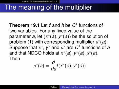
Theorem 19.1 Let f and h be C1 functions oftwo variables. For any fixed value of theparameter a, let (x∗(a), y∗(a)) be the solution ofproblem (1) with corresponding multiplier µ∗(a).Suppose that x∗, y∗ and µ∗ are C1 functions of aand that NDCQ holds at x∗(a), y∗(a), µ∗(a).Then
µ∗(a) =dda
f (x∗(a), y∗(a))
Yu Ren Mathematical Economics: Lecture 14
math
Chapter 19: Constrained Optimization II
Example 19.1
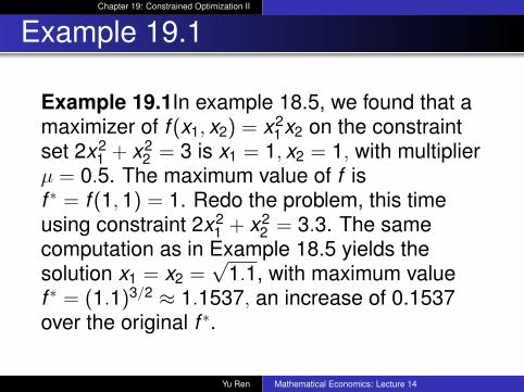
Example 19.1In example 18.5, we found that amaximizer of f (x1, x2) = x2
1 x2 on the constraintset 2x2
1 + x22 = 3 is x1 = 1, x2 = 1, with multiplier
µ = 0.5. The maximum value of f isf ∗ = f (1,1) = 1. Redo the problem, this timeusing constraint 2x2
1 + x22 = 3.3. The same
computation as in Example 18.5 yields thesolution x1 = x2 =
√1.1, with maximum value
f ∗ = (1.1)3/2 ≈ 1.1537, an increase of 0.1537over the original f ∗.
Yu Ren Mathematical Economics: Lecture 14
math
Chapter 19: Constrained Optimization II
Example 19.1
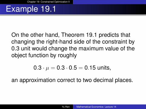
On the other hand, Theorem 19.1 predicts thatchanging the right-hand side of the constraint by0.3 unit would change the maximum value of theobject function by roughly
0.3 · µ = 0.3 · 0.5 = 0.15 units,
an approximation correct to two decimal places.
Yu Ren Mathematical Economics: Lecture 14
math
Chapter 19: Constrained Optimization II
Several Equality Constraints
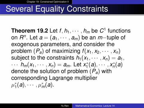
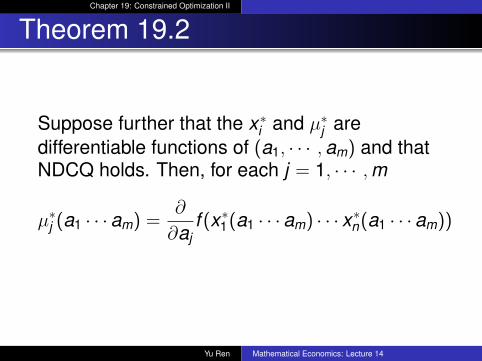
Theorem 19.2 Let f ,h1, · · · ,hm be C1 functionson Rn. Let a = (a1, · · · ,am) be an m−tuple ofexogenous parameters, and consider theproblem (Pa) of maximizing f (x1, x2, · · · , xn)subject to the constraints h1(x1, · · · , xn) = a1,· · · hm(x1, · · · , xn) = am. Let x∗1(a), · · · , x∗n(a)denote the solution of problem (Pa) withcorresponding Lagrange multiplierµ∗1(a), · · · , µ∗m(a).
Yu Ren Mathematical Economics: Lecture 14
math
Chapter 19: Constrained Optimization II
Theorem 19.2
Suppose further that the x∗i and µ∗j aredifferentiable functions of (a1, · · · ,am) and thatNDCQ holds. Then, for each j = 1, · · · ,m
µ∗j (a1 · · · am) =∂
∂ajf (x∗1(a1 · · · am) · · · x∗n(a1 · · · am))
Yu Ren Mathematical Economics: Lecture 14
math
Chapter 19: Constrained Optimization II
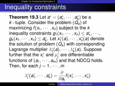
Inequality constraintsTheorem 19.3 Let a∗ = (a∗1, · · · ,a∗k) be ak−tuple. Consider the problem (Qa) ofmaximizing f (x1, · · · , xn) subject to the kinequality constraints g1(x1, · · · , xn) ≤ a∗1, · · · ,gk(x1, · · · , xn) ≤ a∗k . Let x∗1(a), · · · , x∗n(a) denotethe solution of problem (Qa) with correspondingLagrange multiplier λ∗1(a), · · · , λ∗k(a). Supposefurther that the x∗i and µ∗j are differentiablefunctions of (a1, · · · ,am) and that NDCQ holds.Then, for each j = 1, · · · ,m
λ∗j (a∗1, · · · ,a∗k) =
∂
∂ajf (x∗1 , · · · , x∗n)
Yu Ren Mathematical Economics: Lecture 14
math
Chapter 19: Constrained Optimization II
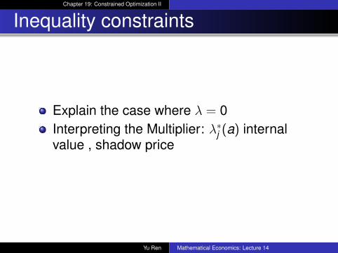
Inequality constraints
Explain the case where λ = 0Interpreting the Multiplier: λ∗j (a) internalvalue , shadow price
Yu Ren Mathematical Economics: Lecture 14
math
Chapter 19: Constrained Optimization II
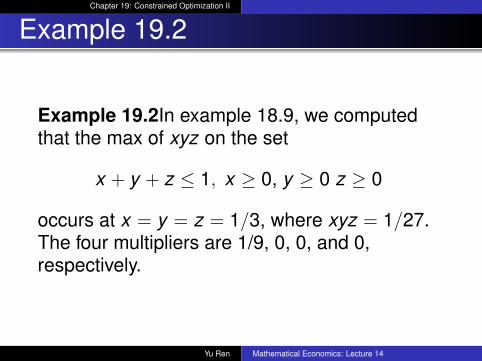
Example 19.2
Example 19.2In example 18.9, we computedthat the max of xyz on the set
x + y + z ≤ 1, x ≥ 0, y ≥ 0 z ≥ 0
occurs at x = y = z = 1/3, where xyz = 1/27.The four multipliers are 1/9, 0, 0, and 0,respectively.
Yu Ren Mathematical Economics: Lecture 14
math
Chapter 19: Constrained Optimization II
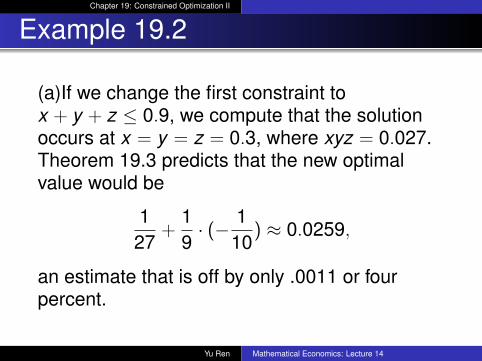
Example 19.2
(a)If we change the first constraint tox + y + z ≤ 0.9, we compute that the solutionoccurs at x = y = z = 0.3, where xyz = 0.027.Theorem 19.3 predicts that the new optimalvalue would be
127
+19· (− 1
10) ≈ 0.0259,
an estimate that is off by only .0011 or fourpercent.
Yu Ren Mathematical Economics: Lecture 14
math
Chapter 19: Constrained Optimization II
Example 19.2
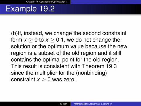
(b)If, instead, we change the second constraintform x ≥ 0 to x ≥ 0.1, we do not change thesolution or the optimum value because the newregion is a subset of the old region and it stillcontains the optimal point for the old region.This result is consistent with Theorem 19.3since the multiplier for the (nonbinding)constraint x ≥ 0 was zero.
Yu Ren Mathematical Economics: Lecture 14
math
Chapter 19: Constrained Optimization II
Envelope Theorems
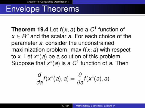
Theorem 19.4 Let f (x ;a) be a C1 function ofx ∈ Rn and the scalar a. For each choice of theparameter a, consider the unconstrainedmaximization problem: max f (x ;a) with respectto x. Let x∗(a) be a solution of this problem.Suppose that x∗(a) is a C1 function of a. Then
dda
f (x∗(a),a) =∂
∂af (x∗(a),a)
Yu Ren Mathematical Economics: Lecture 14
math
Chapter 19: Constrained Optimization II
Example 19.3
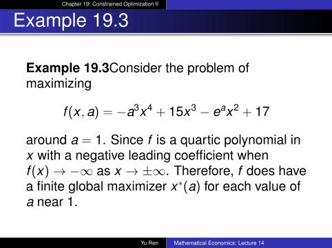
Example 19.3Consider the problem ofmaximizing
f (x ,a) = −a3x4 + 15x3 − eax2 + 17
around a = 1. Since f is a quartic polynomial inx with a negative leading coefficient whenf (x)→ −∞ as x → ±∞. Therefore, f does havea finite global maximizer x∗(a) for each value ofa near 1.
Yu Ren Mathematical Economics: Lecture 14
math
Chapter 19: Constrained Optimization II
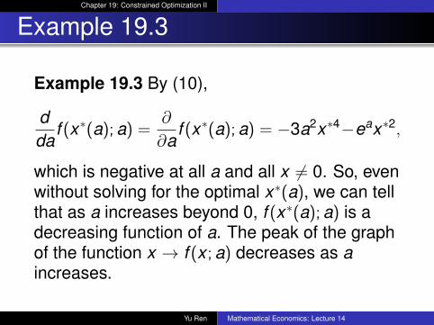
Example 19.3
Example 19.3 By (10),
dda
f (x∗(a);a) =∂
∂af (x∗(a);a) = −3a2x∗4−eax∗2,
which is negative at all a and all x 6= 0. So, evenwithout solving for the optimal x∗(a), we can tellthat as a increases beyond 0, f (x∗(a);a) is adecreasing function of a. The peak of the graphof the function x → f (x ;a) decreases as aincreases.
Yu Ren Mathematical Economics: Lecture 14
math
Chapter 19: Constrained Optimization II
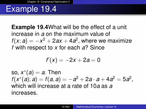
Example 19.4
Example 19.4What will be the effect of a unitincrease in a on the maximum value off (x ;a) = −x2 + 2ax + 4a2, where we maximizef with respect to x for each a? Since
f ′(x) = −2x + 2a = 0
so, x∗(a) = a. Thenf (x∗(a);a) = f (a,a) = −a2 + 2a · a + 4a2 = 5a2,which will increase at a rate of 10a as aincreases.
Yu Ren Mathematical Economics: Lecture 14
math
Chapter 19: Constrained Optimization II
Example 19.4
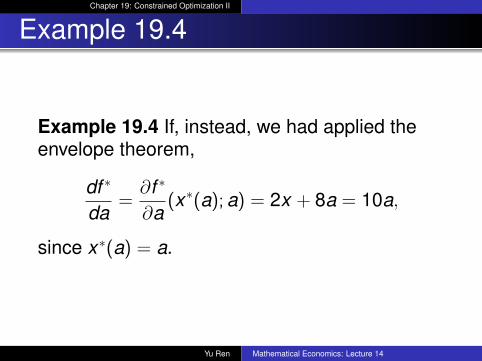
Example 19.4 If, instead, we had applied theenvelope theorem,
df ∗
da=∂f ∗
∂a(x∗(a);a) = 2x + 8a = 10a,
since x∗(a) = a.
Yu Ren Mathematical Economics: Lecture 14
math
Chapter 19: Constrained Optimization II
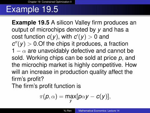
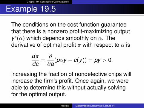
Example 19.5Example 19.5 A silicon Valley firm produces anoutput of microchips denoted by y and has acost function c(y), with c′(y) > 0 andc′′(y) > 0.Of the chips it produces, a fraction1− α are unavoidably defective and cannot besold. Working chips can be sold at price p, andthe microchip market is highly competitive. Howwill an increase in production quality affect thefirm’s profit?The firm’s profit function is
π(p, α) = maxy
[pαy − c(y)],
Yu Ren Mathematical Economics: Lecture 14
math
Chapter 19: Constrained Optimization II
Example 19.5
The conditions on the cost function guaranteethat there is a nonzero profit-maximizing outputy∗(α) which depends smoothly on α. Thederivative of optimal profit π with respect to α is
dπda
=∂
∂a(pαy − c(y)) = py > 0.
increasing the fraction of nondefective chips willincrease the firm’s profit. Once again, we wereable to determine this without actually solvingfor the optimal output.
Yu Ren Mathematical Economics: Lecture 14
math
Chapter 19: Constrained Optimization II
Constrained Problems
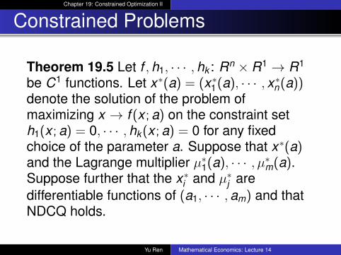
Theorem 19.5 Let f ,h1, · · · ,hk : Rn × R1 → R1
be C1 functions. Let x∗(a) = (x∗1(a), · · · , x∗n(a))denote the solution of the problem ofmaximizing x → f (x ;a) on the constraint seth1(x ;a) = 0, · · · ,hk(x ;a) = 0 for any fixedchoice of the parameter a. Suppose that x∗(a)and the Lagrange multiplier µ∗1(a), · · · , µ∗m(a).Suppose further that the x∗i and µ∗j aredifferentiable functions of (a1, · · · ,am) and thatNDCQ holds.
Yu Ren Mathematical Economics: Lecture 14
math
Chapter 19: Constrained Optimization II
Constrained Problems
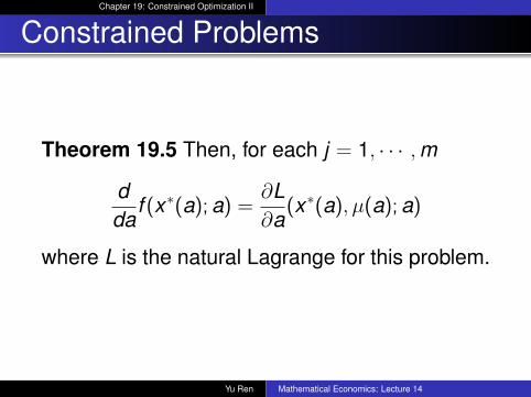
Theorem 19.5 Then, for each j = 1, · · · ,m
dda
f (x∗(a);a) =∂L∂a
(x∗(a), µ(a);a)
where L is the natural Lagrange for this problem.
Yu Ren Mathematical Economics: Lecture 14
math
Chapter 19: Constrained Optimization II
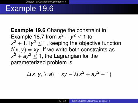
Example 19.6
Example 19.6 Change the constraint inExample 18.7 from x2 + y2 ≤ 1 tox2 + 1.1y2 ≤ 1, keeping the objective functionf (x , y) = xy . If we write both constraints asx2 + ay2 ≤ 1, the Lagrangian for theparameterized problem is
L(x , y , λ;a) = xy − λ(x2 + ay2 − 1)
Yu Ren Mathematical Economics: Lecture 14
math
Chapter 19: Constrained Optimization II
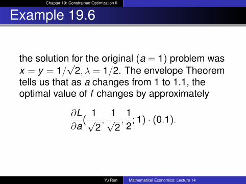
Example 19.6
the solution for the original (a = 1) problem wasx = y = 1/
√2, λ = 1/2. The envelope Theorem
tells us that as a changes from 1 to 1.1, theoptimal value of f changes by approximately
∂L∂a
(1√2,
1√2,12;1) · (0.1).
Yu Ren Mathematical Economics: Lecture 14
math
Chapter 19: Constrained Optimization II
Example 19.6
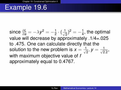
since ∂L∂a = −λy2 = −1
2 · (1√2)2 = −1
4, the optimalvalue will decrease by approximately .1/4=.025to .475. One can calculate directly that thesolution to the new problem is x = 1√
2, y = 1√
2.2,
with maximum objective value of fapproximately equal to 0.4767.
Yu Ren Mathematical Economics: Lecture 14
math
Chapter 19: Constrained Optimization II
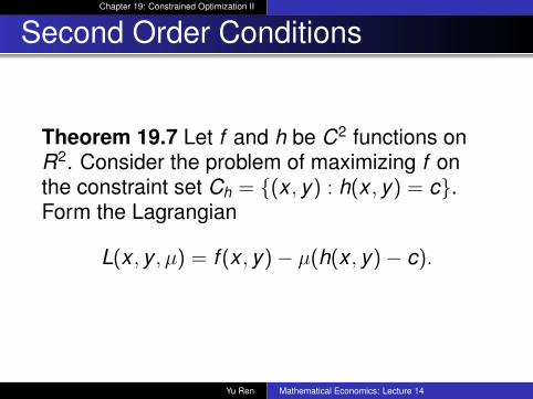
Second Order Conditions
Theorem 19.7 Let f and h be C2 functions onR2. Consider the problem of maximizing f onthe constraint set Ch = {(x , y) : h(x , y) = c}.Form the Lagrangian
L(x , y , µ) = f (x , y)− µ(h(x , y)− c).
Yu Ren Mathematical Economics: Lecture 14
math
Chapter 19: Constrained Optimization II
Second Order Conditions
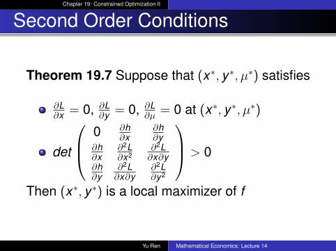
Theorem 19.7 Suppose that (x∗, y∗, µ∗) satisfies
∂L∂x = 0, ∂L
∂y = 0, ∂L∂µ = 0 at (x∗, y∗, µ∗)
det
0 ∂h∂x
∂h∂y
∂h∂x
∂2L∂x2
∂2L∂x∂y
∂h∂y
∂2L∂x∂y
∂2L∂y2
> 0
Then (x∗, y∗) is a local maximizer of f
Yu Ren Mathematical Economics: Lecture 14
math
Chapter 19: Constrained Optimization II
Second Order Conditions
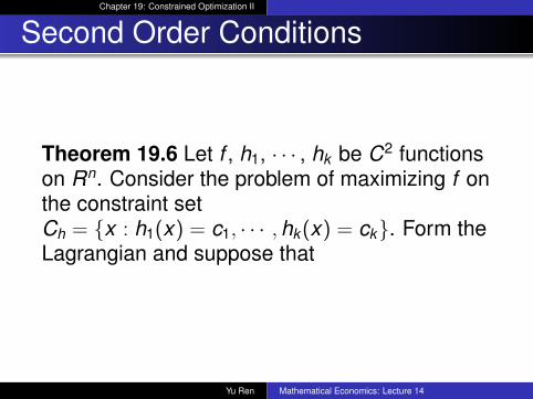
Theorem 19.6 Let f , h1, · · · , hk be C2 functionson Rn. Consider the problem of maximizing f onthe constraint setCh = {x : h1(x) = c1, · · · ,hk(x) = ck}. Form theLagrangian and suppose that
Yu Ren Mathematical Economics: Lecture 14
math
Chapter 19: Constrained Optimization II
Second Order Conditions
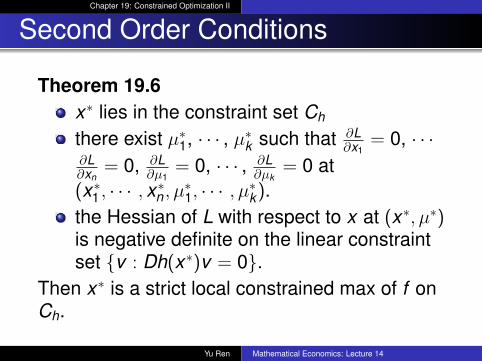
Theorem 19.6x∗ lies in the constraint set Ch
there exist µ∗1, · · · , µ∗k such that ∂L∂x1
= 0, · · ·∂L∂xn
= 0, ∂L∂µ1
= 0, · · · , ∂L∂µk
= 0 at(x∗1 , · · · , x∗n , µ∗1, · · · , µ∗k).the Hessian of L with respect to x at (x∗, µ∗)is negative definite on the linear constraintset {v : Dh(x∗)v = 0}.
Then x∗ is a strict local constrained max of f onCh.
Yu Ren Mathematical Economics: Lecture 14
math
Chapter 19: Constrained Optimization II
Second Order Conditions
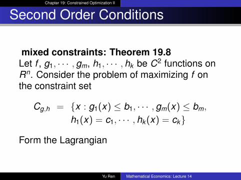
mixed constraints: Theorem 19.8Let f , g1, · · · ,gm, h1, · · · ,hk be C2 functions onRn. Consider the problem of maximizing f onthe constraint set
Cg,h = {x : g1(x) ≤ b1, · · · ,gm(x) ≤ bm,
h1(x) = c1, · · · ,hk(x) = ck}
Form the Lagrangian
Yu Ren Mathematical Economics: Lecture 14
math
Chapter 19: Constrained Optimization II
Second Order ConditionsTheorem 19.8
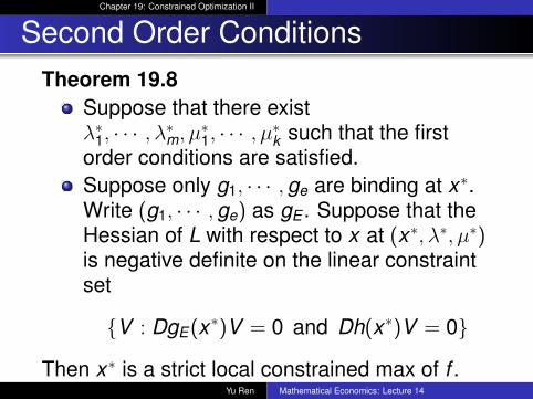
Suppose that there existλ∗1, · · · , λ∗m, µ∗1, · · · , µ∗k such that the firstorder conditions are satisfied.Suppose only g1, · · · ,ge are binding at x∗.Write (g1, · · · ,ge) as gE . Suppose that theHessian of L with respect to x at (x∗, λ∗, µ∗)is negative definite on the linear constraintset
{V : DgE(x∗)V = 0 and Dh(x∗)V = 0}
Then x∗ is a strict local constrained max of f .Yu Ren Mathematical Economics: Lecture 14
math
Chapter 19: Constrained Optimization II
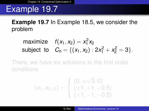
Example 19.7Example 19.7 In Example 18.5, we consider theproblem
maximize f (x1, x2) = x21 x2
subject to Ch = {(x1, x2) : 2x21 + x2
2 = 3}.
There, we have six solutions to the first orderconditions
(x1, x2, µ) =
(0,±√
3,0)(±1,+1,+0.5)(±1,−1,−0.5)
Yu Ren Mathematical Economics: Lecture 14
math
Chapter 19: Constrained Optimization II
Example 19.7
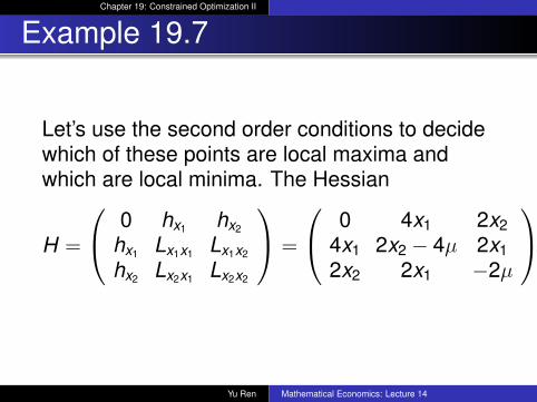
Let’s use the second order conditions to decidewhich of these points are local maxima andwhich are local minima. The Hessian
H =
0 hx1 hx2
hx1 Lx1x1 Lx1x2
hx2 Lx2x1 Lx2x2
=
0 4x1 2x24x1 2x2 − 4µ 2x12x2 2x1 −2µ
Yu Ren Mathematical Economics: Lecture 14
math
Chapter 19: Constrained Optimization II
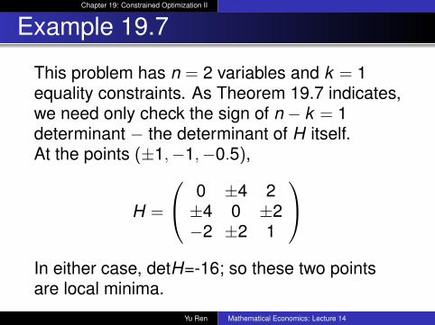
Example 19.7
This problem has n = 2 variables and k = 1equality constraints. As Theorem 19.7 indicates,we need only check the sign of n − k = 1determinant − the determinant of H itself.At the points (±1,−1,−0.5),
H =
0 ±4 2±4 0 ±2−2 ±2 1
In either case, detH=-16; so these two pointsare local minima.
Yu Ren Mathematical Economics: Lecture 14
math
Chapter 19: Constrained Optimization II
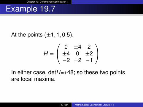
Example 19.7
At the points (±1,1,0.5),
H =
0 ±4 2±4 0 ±2−2 ±2 −1
In either case, detH=+48; so these two pointsare local maxima.
Yu Ren Mathematical Economics: Lecture 14
math
Chapter 19: Constrained Optimization II
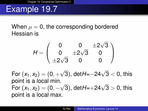
Example 19.7
When µ = 0, the corresponding borderedHessian is
H =
0 0 ±2√
30 ±2
√3 0
±2√
3 0 0
For (x1, x2) = (0,+
√3), detH=−24
√3 < 0, this
point is a local min.For (x1, x2) = (0,−
√3), detH=+24
√3 > 0, this
point is a local max.
Yu Ren Mathematical Economics: Lecture 14
math
Chapter 19: Constrained Optimization II
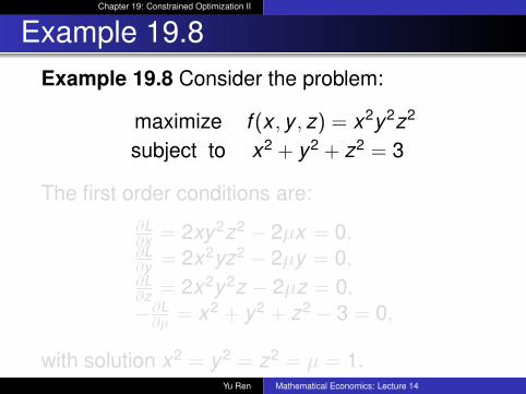
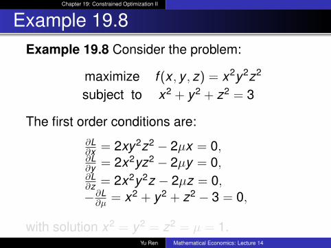
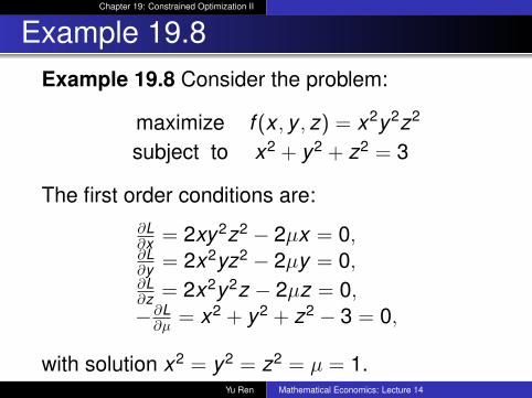
Example 19.8Example 19.8 Consider the problem:
maximize f (x , y , z) = x2y2z2
subject to x2 + y2 + z2 = 3
The first order conditions are:∂L∂x = 2xy2z2 − 2µx = 0,∂L∂y = 2x2yz2 − 2µy = 0,∂L∂z = 2x2y2z − 2µz = 0,−∂L∂µ = x2 + y2 + z2 − 3 = 0,
with solution x2 = y2 = z2 = µ = 1.Yu Ren Mathematical Economics: Lecture 14
math
Chapter 19: Constrained Optimization II
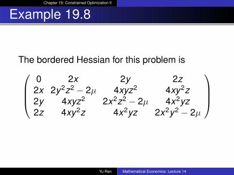
Example 19.8
The bordered Hessian for this problem is0 2x 2y 2z
2x 2y2z2 − 2µ 4xyz2 4xy2z2y 4xyz2 2x2z2 − 2µ 4x2yz2z 4xy2z 4x2yz 2x2y2 − 2µ
Yu Ren Mathematical Economics: Lecture 14
math
Chapter 19: Constrained Optimization II
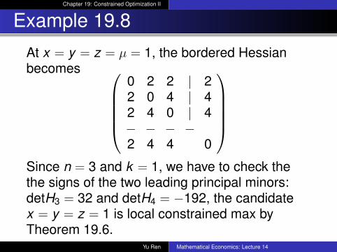
Example 19.8
At x = y = z = µ = 1, the bordered Hessianbecomes
0 2 2 | 22 0 4 | 42 4 0 | 4− − − −2 4 4 0
Since n = 3 and k = 1, we have to check thethe signs of the two leading principal minors:detH3 = 32 and detH4 = −192, the candidatex = y = z = 1 is local constrained max byTheorem 19.6.
Yu Ren Mathematical Economics: Lecture 14


