


330
B385No
.
sn
FACULTY WORKINGPAPER NO. 1173
Maturity and Nonstationarity of Convertible
Bond Beta: Theory and Evidence
Randolph P. Beatty
Cheng F. Lee
K. C. Chen
College of Commerce and Business Adhminii
Bureau of Economic and Business ResearchUniversity of Illinois, Urbana-Champaign


BEBRFACULTY WORKING PAPER NO. 1173
College of Commerce and Business Administration
University of Illinois at Urbana-Champaign
August, 1985
Maturity and Nonstationarity of ConvertibleBond Beta: Theory and Evidence
Randolph P. BeattyUniversity of Pennsylvania
Cheng F. Lee, ProfessorDepartment of Finance
K. C. Chen, Assistant ProfessorDepartment of Finance
Original version of this paper has been presented at 1984 TIMS/ORSA
annual meeting at San Francisco, May 13-16, 1984.


Abstract
This paper has considered the return generating process of conver-
tible bonds. An analytical model of the return generating processes
of convertible bonds was developed. The model combines the capital
asset pricing model and the Black-Scholes option pricing model to pro-
duce empirically testable assertions concerning the effect of changes
in time on systematic risk estimates. An empirical method is
described which allows identification of systematic changes in the
time pattern of convertible security returns. The results of the
variable mean response random coefficient regression model with time
trend indicate that systematic risk for a significant number of con-
vertible securities decline over time.

Digitized by the Internet Archive
in 2011 with funding from
University of Illinois Urbana-Champaign
http://www.archive.org/details/maturitynonstati1173beat

I . Introdu ction
According to the Sharpe (1964), Lintner (1965) and Mossin (1966)
capital asset pricing model (CAPM), an investor's objective is to
maximize his expected utility conditional on his wealth endowment and
risk preferences. In the one-period CAPM, systematic risk (g.) por-
trays the risk-return parameter of interest for portfolio construc-
tion. In this general equilibrium framework, the investor is faced
with the problem of estimating the systematic risk of particular
assets. Historically, the ex post returns on particular assets have
been regressed on an ex post estimate of the return on the market to
obtain estimates of systematic risk. It should be emphasized that a
time series estimate of systematic risk is not a direct result of the
CAPM. Instead, the time series estimate implicitly assumes a sta-
tionary non-stochastic systematic risk parameter. The purpose of this
research is to suggest theoretical and empirical results which
question the validity of the assumption of stationary non-stochastic
systematic risk paremeters for a subset of all risky assets, conver-
tible bonds.
In the next section, a review of convertible security valuation
and random coefficient models are presented as background. In the
third section, an analytical framework for derivation of empirically
testable hypotheses is summarized. Section IV derives the four-step
Hildreth-Houck estimator for the variable mean response random coef-
ficient regression model with time trend. In Section V, the results
of the empirical tests are presented. In Section VI, a section sum-
marizing and concluding this work is offered.

-2-
I I . Review of Convertible Security Valuation and Applications o f
Random Coefficient Models
Convertible security valuation models have evolved with advances
in finance theory. The earliest models of convertible security
valuation were graphical representations (e.g., Brigham (1966)) and
equations with numerous exogeneously specified variables (e.g.,
Baumol, Malkiel and Quandt (1966) and Poensgen (1965, 1966). In more
recent developments, the option pricing methodology has been employed
by Ingersoll (1977) and Brennan and Schwartz (1977) to consider the
valuation problem facing investors. The common theme of all these
valuation methodologies relies on the observation that a convertible
security is a combination of a straight debt value and a premium paid
for the conversion privilege. In the following section, this decom-
position of convertible security value will be employed to consider
the nature of the return generating process of a convertible security.
A second line of finance research has investigated the empirical
attributes of the return generating processes of various risky assets.
With the introduction of the market model, the risk-return structure
of equity securities was investigated by numerous authors. In a
number of endeavors, beta stationarity was the major research
question. Blume (1971, 1975) and Klemkosky and Martin (1975) have
considered the tendency of beta coefficient estimates to regress
toward their mean. In a seminal work on the random coefficient model,
Fabozzi and Francis (1978) found a significant number of equity
securities that displayed return generating processes that may be
characterized as possessing a random coefficient. Following Fabozzi
and Francis (1978) , the use of the random coefficient model to

-3-
describe the observable returns of risky assets has been considered by
a series of authors (e.g., Sunder (1980), Lee and Chen (1982), and
Alexander, Benson and Eger (1982)). This work extends the random
coefficient regression model studies to convertible bonds. In the
next section, the Black-Scholes (1973) option pricing model is blended
with the capital asset pricing model (CAPM) to derive empirically
testable assertions for convertible bonds.
III. The Model and Its Analysis
Using continuous-time contingent-claim analysis, Ingersoll [1977]
has derived a pricing model for a non-callable, coupon-bearing, con-
vertible bond in Theorem V of his paper as follows:
G(V,i;B,C,q) = D(V,t;B,C) + W(qV,T;B) (1)
where G = the value of a non-callable, coupon bearing convertible bond;
D the value of an ordinary bond;
W = the value of a warrant;
V = the market value of the firm;
B = the principal on the ordinary bond;
C = coupon payment;
t = the time to maturity;
q e n/(n+N), the dilution factor when there are N shares of com-mon stock outstanding and the convertible issue can be
exchanged, in aggregate, for n shares.
Equation (1) states that a non-callable, coupon-bearing convertible
bond is equal in value to a portfolio consisting of an ordinary bond
with the same coupon, principal, and maturity plus a warrant entitling

-4-
the owners to purchase the same fraction of the equity of the firm
upon an exercise payment equal to the principal on the bond.
Given the equilibrium valuation relationship in (1), the rela-
tionship between the systematic risks of the three assets can be
easily expressed as
6G=| 6 D+ ! BW < 2 >
where the systematic risk of a non-callable, coupon bearing, conver-
tible bond is simply the value-weighted average of the systematic
risks of an ordinary coupon bond and a warrant respectively.
Recently, Galai and Schneller [1978 J have derived the value of a
warrant as follows:
W = C(l-q) (3)
where C is the premium of a call option which has the same charac-
teristics as the warrant. Eq. (3) states that the value of a warrant
is equal to the value of the call adjusted by the dilution effect.
Since the return on the warrant is always (1-q) the return on the call
option, the systematic risk of the warrant must equal the systematic
risk of the call option.
6 W= 6
C(4)
Furthermore, Galai and Masulis [1976 J have linked the systematic risk
of a call option with the systematic risk of the underlying stock as
follows:
6c =n8
s(5)

-5-
where n is the elasticity of call premium with respect to the value of
the underlying stock.
Substituting (4) and (5) into (2) yields
8G
= aBD
+ (l-a)n3s
(6)
where a = — . The systematic risk of a non-callable, coupon bearing,
convertible bond is a weighted average of the systematic risk of the
straight coupon bond and the systematic risk of the stock multiplied
by an elasticity term. Even if the systematic risk of the stock is
stationary, the systematic risk of the convertible bond will generally
be non-stationary because of the presence of the elasticity term.
Therefore, a non-stationary instead of a stationary market model
should be used to estimate the systematic risk of convertible bond.
Furthermore, as shown by Ingersoll and Galai and Masulis that
!£ < o ^ > i* >3t
S U' 3t ' U
' 3t ' U
36 D>„,
3SS
(7)
37 7 °» and lf < °»
36G
the sign of —r— is indeterminate. To help understand the effect of a
change in time x on the systematic risk of the convertible bond,
further examination of the nature of the convertible bond is necessary.
Since most convertible bonds are issued with a call provision, in
what follows we will bring this call feature into our analysis. As
Ingersoll [1977] has proven his Theorem VII, whenever it is optimal to
voluntarily convert a non-callable convertible bond, it will also be
optimal to convert a callable, convertible bond which is otherwise

-6-
identical. Therefore, the preceding analysis can be applied to
callable convertible bonds also. Furthermore, Ingersoll has shown
that if the perfect markets, no dividends, and constant conversion
terms assumptions are valid, then a callable convertible will never be
converted except at maturity or call. If voluntary conversion is
allowed, Ingersoll has shown that voluntary conversion of a conver-
tible bond will occur only if the current dividend yield on the stock
exceeds the current yield on the bond. Thus, a callable convertible
bond will behave more like the stock if the current dividend yield on
the stock is close to or exceeds the current yield on the bond; other-
wise, it will behave more like the straight bond. In the former case,
the effect of a change in time on the second term in (6) dominates the
effect of a change in time on the first term. Therefore, 93^/St < 0.
>In the latter case, 33„/8t "7 0. However, Weinstein [1983] has shown
that 33 n/3T > if coupon rate on the bond is greater than the risk-
free rate and the value of the firm exceeds the value of a risk-free
bond with the same promised payments as the corporate bond. When the
convertible bond behaves more like the straight bond, it is more
likely that 83 p/3t > 0, given Weinstein' s results.
IV. Research Method
A general linear regression model with random coefficient is pre-
sented in equation (8) below:
y(t) = Z 3,(t)X,(t) (8)
X-lA x
where

-7-
y(t) = the t— observation of the dependent variable;
x- (t) = the t— observation of the X independentvariable;
3 (t) = the random coefficient of the X independentvariable;
t = 1, ..., T (Singh, Nagar, Choudhry and Raj (1976), p.
342).
The random coefficient is modeled in equation (9) as follows:
3x(t) = B
x+ ct
xfx(t) + e
x(t) (9)
where
f (t) is a function of time, t;A
3, is the constant slope through time;
a. is the coefficient of the time trend of the randomcoefficient 3,(t);
e.(t) is a random component associated with 3 (t).
This model of the random coefficient can be introduced into equation
(8) to obtain equation (10):
A Ay(t) = Z 3,x. (t) + E a.f. (t)x, (t) + w_ (10)
X=lA x
X=lx x x t
whereA
w = Z e. (t)x, (t).t
X=lx x
To consider the time trend of convertible security systematic risk, an
adaptation of the familiar market model will be estimated. The spe-
cific form of this model in terms of market model is presented in
2equation (11)
:
Vt) =F1+ ?2Rm(t)
+ a lC + a2tR (t) +wnr t (ID

-8-
where
R.(t) is the rates of return on the ith security;
R (t) is the market rates of return:m
t is the time trend.
Equation (11) is transformed into matrix notation in equation (12)
below:
where
r = ze + w (12)
R =R4(2)
Ri(T)_
f
Z =
1 Rm(l) 1 RJ1)
1 R (2) 2 2R (2)m m
1 R (T) T TR (T)m m -
R—
m
tR—
m
w =
w.
w.f- T -*
R =—
m
1 Rju1 r"(2)
m
1 R (T)m
B =
" VJ2
"l
- «2-

-9-
To estimate equation (12), a four-step modified Hildreth-Houck estima-
tor is employed. First, an estimate of w is obtained in equation (13).
w = M R (13)
where
M = I - Z(Z'Z)1Z'.
Next, we consider the matrices of squared elements of w, M and R^ in
equation (14). (The dot, ., indicates that the elements are squared.)
• •
21= H B-jg + n_ = Go + n_ (14)
where
a = 11
f-a22-
n_ = w - Ew.
With the second use of least squares procedures, equation (15) is
obtained:
a = (G'G) """G'w (15)
With equation (15) an estimator of a,, and a ??can be used to develop
an estimate of #• Next, equation (16) can be shown to be a direct
result of the assumptions required to derive equation (14) (Singh,
Nagar, Choudhry and Raj (1976), p. 352).
Erm' = 2£_ (16)
where

-10-
£ = m_H;
$_ = is the squared elements of £_.
Given equation (16), a second estimator of a can be derived from
equation (17).
a* = (G'^G^G'^w (17)
In the fourth stage, o_* is employed to develop an estimate of $_, _$*.
This result permits a final estimate of 3_ in equation (18).
3* = {Z^*"1Z)"1Z 1 9*~1K. (18)
Equation (18)' s estimate of 3 , 3 9 , a and a_ can be tested for sta-
tistical significance in the traditional fashion employing simple
t-tests. In the next section, results of the four-step modified
Hildreth-Houck estimate of the variable mean response random coef-
ficient model with time trend are reported.
V. Empirical Evidence
V.l Data and Model
This section presents the results of the model employing a four-
step Hildreth-Houck estimator of a random coefficient model with time
trend. First, the sample of convertible securities is described.
Then, the random coefficient results are summarized.
Sample selection followed a two-step process. First, the popula-
tion of convertible bonds was defined to be those convertible securi-
ties which were outstanding from 1976 through 1979, inclusive. This
criterion yields 347 convertible bonds. Then, 100 convertible bonds

-11-
were randomly selected. The second step required each of the pre-
viously selected convertible securities to be readily available in the
data collection sources. Three convertible bonds were not listed in the
Commercial and Financial Chronicle for the time period selected.
Thus, the final sample contains 97 convertible bonds.
Once the sample of convertible bonds was established, monthly
price data was assembled from the Commericial and Financial Chronicle .
Upon collection of monthly prices, monthly returns (adjusted for cash
distributions) were created. These monthly returns are the dependent
variable in the random coefficient models. The independent variable
in the random coefficient models was a broadly based value-weighted
index. Monthly returns and market values for U.S. government bonds,
Standard and Poor's High Grade bonds and the CRSP equity securities
were combined to obtain the value-weighted index. With these depen-
dent and independent variables, both the ordinary least squares (OLS)
regression and the random coefficient regression model are estimated
3in terras of equations (19) and (20) respectively.
R._ = a. + .R . + e .«. (19)jt J
PJ mt jt
R.«. = a. + S 4 «.R * + e_ (20)Jt j Jt mt jt
where
jt= 3 + Yt + n
t
V.2 Hypothesis to be Tested
As discussed in Section III, a convertible bond will behave more
like the stock if the current dividend yield on the stock exceeds the

-12-
current yield on the bond. Therefore, 33-/3T < 0. The coefficient of
Y in (20) is hypothesized to be negative. When the current dividend
yield on the stock is less than the current yield on the bond, the
convertible bond will behave more like the straight bond. If coupon
rate on the bond is greater than the risk-free rate and the value of
the firm exceeds the value of a risk-free bond with the same promised
payments as the corporate bond, 38_,/3t > 0. Therefore, the coef-
ficient of y in (20) is hypothesized to be positive. For other cases,
the coefficient of y is hypothesized to be negative.
V.3 Empirical Results
Table 1 reports the results. There are 20 convertible bonds that
behave like stock because their dividend yields are greater than cor-
responding current yields. Among them, 14 convertible bonds exhibit
negative y coefficient as hypothesized, while six exhibit positive y
coefficient (only 1 exhibits significant positive y coefficient). In
our sample, there is no single convertible bond whose coupon rate is
greater than the average risk-free rate in 1979, thus the coefficients
of y for 77 convertible bonds whose dividend yield are less than
corresponding current yield are hypothesized to be negative or zero.
As shown in Table 1, there are 77 convertible bonds which behave more
like the straight bonds. Among them, 42 exhibit significant negative
Y and 28 insignificant. However, there are 33 convertible bonds which
exhibit positive y coefficient, but only 10 show statistical signifi-
cance.

1 105 23
5 14
9 28
-13-
Table 1
Behave Like Stock Behave Like Bond
Significant positive y:Insignificant positive y
:
Significant negative y :
Insignificant negative y
:
Total 20 11
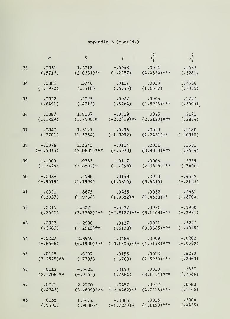
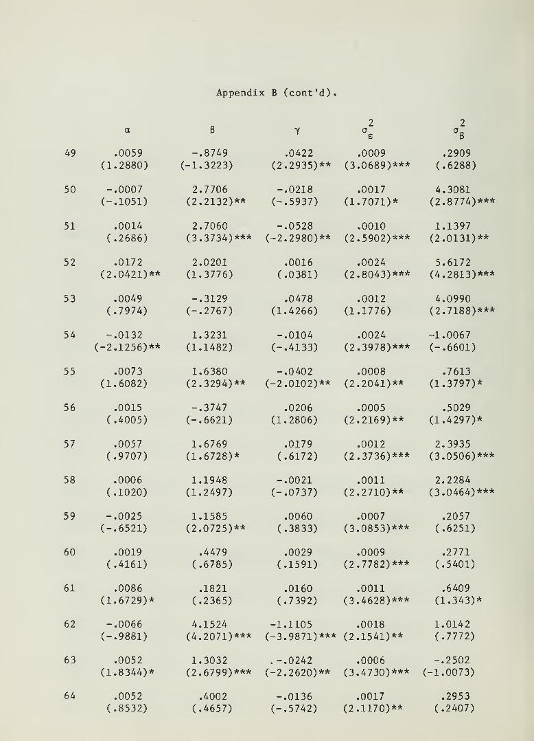
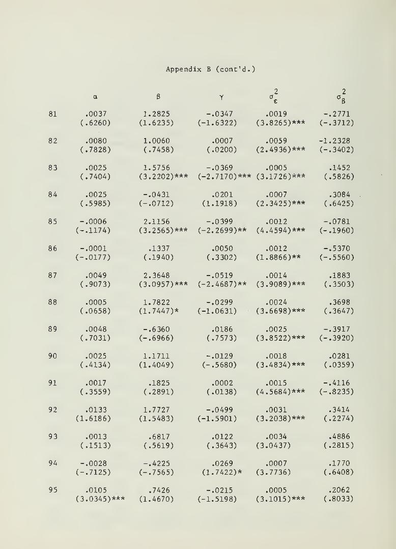
Results of equation (19) are presented in Appendix A and results
of equation (20) are presented in Appendix B. In Appendix A, the
market model results suggest that convertible security systematic risk
is slightly below the systematic risk of the entire market (8 = .8104)
In, similar fashion to estimate of equity security systematic risk with
monthly data, a significant proportion of estimated systematic risk
parameters are different from zero at the 5% a-level (65%). Summary
results of Appendix B are listed in Table 2.
Table 2
RandomSlope Coefficient
Intercept Slope (time trend) Parametera 6 y
1% 3 17 9 105% 9 13 14 4
10% 7 9 7 6
Insignificant 78 58 67 75
There are 30 out of 97 convertible bonds with significant y-
coefficient estimates under 10 percent significance level. Eleven of
these 30 convertible bonds exhibit a positive estimated y-coef f icient.
The company names of these 30 convertible bonds and their coupon rates
are listed in Appendix C. These results imply that maturity can be
important in estimating the beta coefficients of convertible bonds. In
twenty out of 97 firms, the random coefficient parameter is significant

-14-
at the 10% a-level. This evidence suggests that a fixed coefficient
ordinary least squares estimate of a convertible bond systematic risk may
exhibit significant levels of measurement error. Thus, the assumption
of convertible bond systematic risk, stationarity may not be descrip-
tively accurate for a significant subset of convertible securities.
VI. Summary and Conclusions
This paper has considered the return generating process of conver-
tible bonds. An analytical model of the return generating processes
of convertible bonds was developed. The model combines the capital
asset pricing model and the Black-Scholes option pricing model to pro-
duce empirically testable assertions concerning the effect of changes
in time on systematic risk estimates. An empirical method is
described which allows identification of systematic changes in the
time pattern of convertible security returns. The results of the
variable mean response random coefficient regression model with time
trend indicate that systematic risk for a significant number of con-
vertible securities decline over time. Based upon the information of
dividend yield, corporate, average risk-free rate and the sign of
estimated y , 97 convertible bonds are classified into either behaving
like stock or behaving like bond.
These results also suggest that an ordinary least squares estimate
of convertible security systematic risk may produce imprecise estimates.
This work has documented a time trend for a sizable proportion of the
convertible bonds in the sample. When considering the application of
the market model for systematic risk estimation with convertible
bonds, the addition of a time parameter may provide a statistically
significant explanatory variable for a number of convertible securities.

-15-
FQQTNQTES
This seems like a reasonable assumption. Using Compustat data,Weinstein [1983] has found that the value of the firm exceeds the value
of debt for most firms.
2The research method presented in Section IV is a direct applica-
tion of Singh, Nagar, Choudhry and Raj's (1976) generalized randomcoefficient regression model.
3The models defined in equations (19) and (20) are only special
cases of the model defined in equation (11).

-16-
REFERENCES
Alexander, G. J., Benson, P. G. and Eger, C. E. (1982). "TimingDecisions and the Behavior of Mutual Fund Systematic Risk."Journal of Financial and Quantitative Analysis 17: 579-602.
Black, F. and Scholes, M. (1973). "The Pricing of Options andCorporate Liabilities." Journal of Political Economy 81: 637-659.
Blume, M. E. (1971). "On the Assessment of Risk." The Journal of
Finance 26: 1-10.
Blume, M. E. (1975). "Beta and Their Regression Tendencies." TheJournal of Finance 30: 785-795.
Fabozzi, F. J. and Francis, J. C. (1978). "Beta as a Random Co-efficient." Journal of Financial and Quantitative Analysis 13:
101-116.
Galai, Dan and Masulis, Ronald W. (1976). "The Option Pricing Modeland the Risk Factor of Stock." Journal of Financial Economics3: 53-81.
Galai, Dan and Schneller, M. (1978). "Pricing of Warrants and the
Value of the Firm." Journal of Finance 5: 1333-1341.
Hildreth, C. and Houck, I. P. (1968). "Some Estimates for a LinearModel with Random Coefficients." Journal of the AmericanStatistical Association 63: 584-595.
Ingersoll, J. E., Jr. (1977). "A Contingent-Claims Valuation of
Convertible Securities," Journal of Financial Economics 3:
289-322.
Klemkosky, R. C. and Martin, J. D. (1975). "The Adjustment of BetaFactors." Journal of Finance 30: 1123-1128.
Lee, C. F. and Chen, C. (1982). "Beta Stability and Tendency: An
Application of a Variable Mean Response Regression Model."Journal of Economics and Business 34: 201-206.
Litner, J. (1965). "Security Prices, Risk and Maximal Gains fromDiversification." Journal of Finance 20: 587-616.
Malkiel, B. G. (1966). The Term Structure of Interest Rates:Expectations and Behavior Patterns , Princeton University Press,Princeton, N.J.
Mossin, J. (1966). "Equilibrium in a Capital Asset Market."Econometrica 34: 768-783.

-17-
Sharpe, W. F. (1964). "Capital Asset Prices: A Theory of MarketEquilibrium Under Conditions of Risk," Journal of Finance 19:
425-442.
Singh, S. Nagan, A. L. , Choudhry, N. K. and Raj, B. (1976). "On theEstimation of Structural Change: A Generalization of theGeneralized Regression Model." International Economic Review 17:
340-361.
Sunder, S. (1980). "Stationarity of Market Risk: Random CoefficientTests for Individual Common Stocks." Journal of Finance 35:
883-896.
Weinstein, M. (1983) . "Bond Systematic Risk and the Option PricingModel." Journal of Finance 38: 1415-1430.
D/274A

Appendix A
Firm No. t-Ratios Firm No. t-Ratios
1 .3961 1.6551 49 .6085 2.51332 .3147 1.9170 50 1.6815 4.12393 1.3149 3.6084 51 1.1194 3.93334 1.1692 4.8539 52 2.0807 4.40465 .2666 .5302 53 1.8747 4.85486 1.3371 2.7469 54 .8957 2.83867 .3125 1.8939 55 .5238 2.15998 .1210 .6402 56 .3470 1.86349 .7936 2.9380 57 1.9962 6.1222
10 1.7173 6.6268 58 1.3589 4.405811 1.2831 4.0382 59 1.3468 7.083012 .9439 2.6467 60 .6284 2.765613 .3616 1.4437 61 .8089 3.131014 .0359 .4440 62 .3455 .8592
15 1.0482 4.7417 63 -.0024 -.015316 -.0123 -.0243 64 -.0383 -.129617 .5891 1.4670 65 1.3502 3.907818 1.6729 6.4439 66 1.0702 4.161019 1.5633 7.1408 67 1.1109 2.026420 1.0280 2.7122 68 1.7908 4.842121 1.5840 3.8184 69 1.1032 3.067722 1.1827 2.3926 70 -.1296 -.520623 .7757 4.2917 71 .7944 2.991924 .4540 1.4837 72 .0028 .045525 .9874 2.1197 73 1.0490 2.523926 1.7375 3.3726 74 .4553 2.003627 1.3290 4.4478 75 2.2769 5.605028 1.0903 3.5842 76 .4892 .350629 .5911 2.9236 77 .7988 3.974630 -.0333 -1.1627 78 2.3835 4.797831 .8135 4.2518 79 .6355 2.460132 1.9556 4.3754 80 1.2346 4.298533 1.3837 5.2057 81 .0161 .053334 .9282 2.6588 82 1.0863 2.110035 .5174 3.1373 83 .3108 1.733636 -.3749 -.9838 84 .6651 3.210237 .2572 .844 85 .7192 2.925338 1.7200 7.0970 86 .0798 .3618
39 .6407 3.5915 87 .6300 2.248440 .9713 4.0741 88 .8517 2.379541 1.1557 3.0787 89 -.0313 -.091642 .0748 .2218 90 .7300 2.438243 .2171 .6990 91 .0125 .049044 .7181 3.2082 92 .0869 .211345 1.1389 4.0429 93 1.1136 2.664446 -.0111 -.0046 94 .5310 2.631847 .6769 2.6398 95 .0730 .418348 .2398 .8280 96 .5201 3.1255
97 .2253 .5246
8 .8104cv

Appendix B
10
11
12
13
14
15
16
-.0032 1.4592 -.0296 .0011 -.1146(-.6908) (2.3285)** (-1.7527)* (3.9026)** (-.2615)
.0019 2.0170 -.0498 .0003 .1317
(.6758) (4.9422)*** (-4.3734)*** (3.2978)*** (.8354)
-.0032 1.8003 -.0135 .0028 .1237
(-.4142) (1.6951)* (-.4658) (2.2711)** (.0648)
-.0025 2.4003 -.0362 .0006 1.4487(-.5854) (3.2684)*** (-1.6831)* (2.6737)*** (4.3077)***
-.0149 -.0740 -.0004 .0059 -1.9910(-1.9423)* (-.0705) (-.0140) (2.8430)*** (-.6210)
.0040 .5352 .0238 .0044 1.3491(.4030) (.3730) (.5957) (2.5636)*** (.5162)
.0015 -.3902 .0204 .0005 .0761
(.4475) (-.8584) (1.6280) (3.2440)*** (.3362)
.0058 .6853 -.0213 .0006 .3503
(1.5615) (1.2280) (-1.3576) (2.8167)*** (1.1275)
.0108 .8499 -.0048 .0013 .3897(1.9644)** (1.0737) (-.2164) (3.5829)*** (.6782)
.0013 2.0735 -.0227 .0009 1.0764(.2613) (2.6533)*** (-1.0168) (2.6037)*** (2.0079)**
-.0247 .5640 .0052 .0024 -.8419(-3.9024)*** (1.3520) (.3140) (4.0126)*** (-.9219)
.0025 2.4116 -.0455 .0021 .6305
(.3574) (2.4071)** (-1.6351) (3.0191)*** (.5782)
.0063 2.4973 -.0618 .0010 -.1681
(1.4443) (4.3418)*** (-4.0037)*** (3.2324)*** (-.3512)
.0016 .0699 -.0006 .0002 -.0422
(1.0338) (.3508) (-.1068) (3.5451)*** (-.6486)
-.0010 1.1583 -.0054 .0008 .6328
(-.2336) (1.7198)* (-.2836) (2.6651)*** (1.4422)*
.0155 -.7140 .0077 .0057 -2.1868
(1.4203) (-.8254) (1.2450) (1.7815)** (-.4439)

Appendix B (cont'd.)
17
18
19
20
21
22
23
24
25
26
27
28
29
30
31
32
.0152 -1.5284 .0596 .0027 .6272(1.9678)** (-1.3921) (1.9602)** (3.2166)*** (.4937)
.0019 .7382 .0266 .0012 .4217
(.3704) (.9809) (1.2692) (2.6680)*** (.6280)
.0037 .3329 .0349 .0010 -.1613(.8696) (.5881) (2.3012)** (4.3713)*** (-.4710)
.0040 3.4711 -.0680 .0028 -.6358(.5669) (3.7799)*** (-2.7652)*** (3.0912)*** (-.4560)
.0100 2.5315 -.0340 .0022 3.^476(1.2286) (1.9738)** (-.9190) (2.4520)*** (2.5146)***
.0014 2.6851 -.0458 .0044 1.2008(.1414) (1.8773)* (-1.1560) (3.1883)*** (.5634)
.0023 .6503 -.0010 .0002 1.1395(.9107) (1.2422) (-.0614) (.8417) (3.5650)***
.0067 .2659 .0001 .0011 2.0606(1.1932) (.2818) (.0048) (2.3654)*** (2.8846)***
.0073 2.0925 -.0330 .0041 .5987
(.7753) (1.5810) (-.9067) (2.6138)*** (.2496)
.0206 1.0827 .0145 .0041 3.6666(2.0026)** (.6817) (.3209) (1.8164)** (1.0440)
-.0097 1.5751 -.0068 .0017 .3359
(-1.5815) (1.8135)* (-.2842) (3.7696)*** (.4840)
-.0021 2.3770 -.0411 .0010 1.7350(-.3960) (2.6633)*** (-1.5927) (1.9297)** (2.1151)**
-.0031 1.3671 -.0245 .0007 .1989
(-.7540) (2.3524)** (-1.5189) (4.5962)*** (.8157)
.0099 1.1803 -.0350 .0016 .0767
(1.7322)* (1.4927) (-1.6203) (2.8679)*** (.0920)
.0010 1.1958 -.0019 .0007 .0571
(.2575) (2.2093)** (-.8002) (3.8483)*** (.2002)
.0168 2.7768 -.0253 .0044 -.7417
(1.8536)* (2.3156)** (-.7869) (2.2426)** (-.2467)
Appendix B (cont'd.)
33 .0031 1.5518 -.0048 .0014 .1582
(.5716) (2.0231)** (-.2287) (4.4654)*** (.3281)
34 .0081 .5746 .0137 .0018 1.7536(1.1972) (.5416) (.4540) (1.1087) (.7065)
35 .0022 .2025 .0077 .0005 .1797
(.6491)
.0087
(.4213)
1.8107
(.5764) (2.8226)*** (.7004)
36 -.0639 .0025 .4171
(1.1829) (1.7500)* (-2.2409)** (2.6120)*** (.2884)
37 .0047 1.3127 -.0296 .0019 -.1180
(.7701) (1.5754) (-1.3092) (2.2431)** (-.0910)
38 -.0076 2.1345 -.0114 .0011 .1581
(-1.5315) (3.0635)*** (-.5970) (3.8043)*** (.3444)
39 -.0009 .9785 -.0117 .0006 .2359
(-.2425) (1.8532)* (-.7958) (2.6818)*** (.7400)
40 -.0028 .5588 .0148 .0013 -.4549(-.9419) (1.1994) (1.0810) (3.6496) (-.8133)
41 .0021 -.8675 .0465 .0032 -.9631
(.3037) (-.9764) (1.9382)* (4.4533)** (-.8704)
42 .0015 2.3025 -.0637 .0021 -.2980
(.2443) (2.7368)*** (-2.8127)*** (3.1508)*** (-.2921)
43 .0023 -.2096 .0137 .0021 -.3247
(.3660) (-.2515)** (.6103) (3.9665)*** (-.4018)
44 -.0027 2.3949 -.0486 .0009 -.0202
(-.6466) (4.1900)*** (-3.1305)*** (4.5158)*** (-.0689)
45 .0125 .6307 .0155 .0013 .6220
(2.2525)** (.7705) (.6760) (2.5970)*** (.8063)
46 .0112 -.6422 .0150 .0010 .3857
(2.3206)** (-.9155) (.7664) (3.1454)*** (.7886)
47 .0021 2.2270 -.0457 .0012 .0583
(.4243) (3.2609)*** (-2.4462)** (4.7918)*** (.1566)
48 .0055 1.5472 -.0386 .0015 .2506
(.9483) (.9080)* (-1.7270)* (4.1158)*** (.4435)
Appendix B (cont'd).
49 .0059
(1.2880)
50 -.0007(-.1051)
51 .0014
(.2686)
52 .0172(2.0421)**
53 .0049
(.7974)
54 -.0132(-2.1256)**
55 .0073
(1.6082)
56 .0015
(.4005)
57 .0057
(.9707)
58 .0006
(.1020)
59 -.0025(-.6521)
60 .0019
(.4161)
61 .0086
(1.6729)*
62 -.0066(-.9881)
63 .0052(1.8344)*
64 .0052
(.8532)
-.8749(-1.3223)
2.7706(2.2132)**
2.7060(3.3734)***
2.0201(1.3776)
-.3129(-.2767)
1.3231(1.1482)
1.6380(2.3294)**
-.3747(-.6621)
1.6769(1.6728)*
1.1948(1.2497)
1.1585(2.0725)**
.4479
(.6785)
.1821
(.2365)
4.1524(4.2071)***
1.3032(2.6799)***
.4002
(.4657)
.0422
(2.2935)**
-.0218(-.5937)
-.0528(-2.2980)**
.0016
(.0381)
.0478
(1.4266)
-.0104(-.4133)
-.0402(-2.0102)**
.0206
(1.2806)
.0179
(.6172)
-.0021(-.0737)
.0060
(.3833)
.0029
(.1591)
.0160
(.7392)
-1.1105(-3.9871)***
.-.0242(-2.2620)**
-.0136(-.5742)
.0009(3.0689)***
.0017
(1.7071)*
.0010(2.5902)***
.0024(2.8043)***
.0012
(1.1776)
.0024(2.3978)***
.0008(2.2041)**
.0005(2.2169)**
.0012(2.3736)***
.0011(2.2710)**
.0007(3.0853)***
.0009(2.7782)***
.0011(3.4628)***
.0018(2.1541)**
.0006(3.4730)***
.0017(2.1170)**
u6
.2909
(.6288)
4.3081(2.8774)***
1.1397(2.0131)**
5.6172(4.2813)***
4.0990(2.7188)***
-1.0067(-.6601)
.7613
(1.3797)*
.5029
(1.4297)*
2.3935(3.0506)***
2.2284(3.0464)***
.2057
(.6251)
.2771
(.5401)
.6409
(1.343)*
1.0142(.7772)
-.2502(-1.0073)
.2953(.2407)

Appendix B (cont'd.)
e
65 .0099 -.7636 .0625 .0020 .2645
(1.4995) (-.8216) (2.4465)** (3.1114)*** (.2633)
66 .0104 -.3065 .0396 .0011 .2261(2.0948)** (-.4356) (2.0390)** (3.0103)*** (.3977)
67 .0081 -1.0451 .0712 .0043 3.5755(.7783)
•
(-.6531) (1.5697) (1.2073) (.6541)
68 -.0022 -.3774 .0676 .0021 1.0581(-.3068) (-.3612) (2.3080)** (3.4466)*** (1.1317)
69 -.0026 1.9428 -.0334 .0019 1.5045(-.3753) (1.8333)* (-1.1134) (2.5612)*** (1.3077)*
70 .0037 .2407 -.0123 .0012 .1651
(.7344) (.3373) (-.6277) (2.1701)** (.1956)
71 -.0006 1.9285 -.0315 .0014 -.1355(-.1205) (2.7715)*** (-1.6782)* (3.6698)*** (-.2368)
72 .0020 .1854 -.0054 .0001 -.0266(1.9073)* (1.3963) (-1.4770) (2.6853)*** (-.5647)
73 -.0016 -.6628 .0502 .0036 -.6214(-.1964) (-.6164) (1.7401)* (2.1022)** (-.2391)
74 -.0005 -.0325 .0158 .0011 -.1340(-.1111) (-.0529) (.9528) (3.4923)*** (-.2786)
75 .0043 1.4598 .0168 .0017 .5995
(.5995) (1.1698) (.4589) (1.4409)* (2.3108)**
76 -.0824 1.6217 .2063 .0505 -28.3133(-3.2321)*** (.4309) (7.9871)*** (3.0670)*** (-1.1173)
77 -.0044 1.4618 -.0204 .0006 .3750
(-1.1098) (2.4881)** (-1.2340) (3.1694)*** (1.2106)
78 .0113 -.9708 .0974 .0041 .5056
(1.2087) (-.7399) (2.7019)*** (3.9104)*** (.3163)
79 .0020 .6293 -.0028 .0012 .3306
(.3849) (.8385) (-.1350) (4.1949)*** (.7413)
80 .0010 1.9918 -.0222 .0016 .1421
(.16452) (2.4580)** (-.9990) (3.8947)*** (.2266)
Appendix B (cont'd.)
81
82
83
84
85
86
87
88
89
90
91
92
93
94
95
.0037 1.2825 -.0347 .0019 -.2771
(.6260) (1.6235) (-1.6322) (3.8265)*** (-.3712)
.0080 1.0060 .0007 .0059 -1.2328(.7828) (.7458) (.0200) (2.4936)*** (-.3402)
.0025 1.5756 -.0369 .0005 .1452
(.7404) (3.2202)*** (-2.7170)*** (3.1726)*** (.5826)
.0025 -.0431 .0201 .0007 .3084
(.5985) (-.0712) (1.1918) (2.3425)*** (.6425)
-.0006 2.1156 -.0399 .0012 -.0781(-.1174) (3.2565)*** (-2.2699)** (4.4594)*** (-.1960)
-.0001 .1337 .0050 .0012 -.5370(-.0177) (.1940) (.3302) (1.8866)** (-.5560)
.0049 2.3648 -.0519 .0014 .1883
(.9073) (3.0957)*** (-2.4687)** (3.9089)*** (.3503)
.0005 1.7822 -.0299 .0024 .3698
(.0658) (1.7447)* (-1.0631) (3.6698)*** (.3647)
.0048 -.6360 .0186 .0025 -.3917(.7031) (-.6966) (.7573) (3.8522)*** (-.3920)
.0025 1.1711 -.0129 .0018 .0281
(.4134) (1.4049) (-.5680) (3.4834)*** (.0359)
.0017 .1825 .0002 .0015 -.4116
(.3559) (.2891) (.0138) (4.5684)*** (-.8235)
.0133 1.7727 -.0499 .0031 .3414
(1.6186) (1.5483) (-1.5901) (3.2038)*** (.2274)
.0013 .6817 .0122 .0034 .4886
(.1513) (.5619) (.3643) (3.0437) (.2815)
-.0028 -.4225 .0269 .0007 .1770
(-.7125) (-.7565) (1.7422)* (3.7736) (.6408)
.0105 .7426 -.0215 .0005 .2062(3.0345)*** (1.4670) (-1.5198) (3.1015)*** (.8033)

Appendix B (cont'd.)
2 2
96 .0058 .4930 -.0025 .0004 .5663
(1.8518)* (.9579) (-.1672) (2.6425)*** (2.8035)***
97 .0359 .8479 -.0762 .0050 -3.1951
(2.3235)** ( .7806 ) (-2.1316 )** (3.3205)*** (-1.3807)
Average 1.0107 -.0155
*** = significant at 1% level** = significant at 5% level* = significant at 10% level

Appendix C
Coupon Rate and Maturity Date for ConvertibleBonds with Significant Time Trend
CompanyNo. Company Name
1 Alexander's Inc.
2 Allegheny Ludlum Steel4 Aluminum Co. of America
13 Bobbie Brooks, Inc.
17 Chris-Craft Industries, Inc.
19 Computer Sciences Corp.
20 Cooper Laboratories, Inc.
36 Great Northern Wekoosa, Corp.
41 International Minerals and Chemical Corp.42 International Silver Co.
44 Kirsch Co.
47 Maryland Cup Corp.48 Mohawk Data Sciences49 National Can Corp.51 North American Phillips Corp.55 Parker-Hannif in Corp.
62 St. Regis Paper Co.
63 Standex Intl. Corp.
65 Stores Broadcasting Co.
66 Sundstrand Corp.68 Tesorro Petroleum Corp.71 United Brands Co.
73 White Motor Corp.76 Wyly Corp.78 Zapata Corp.83 DPF, Inc.
85 Fischer and Porter Co.
87 Grow Chemical Corp.94 Ryan Homes, Inc.97 Work Wear Corp.
Coupon MaturityRate Date
5.55 96
4.05 81
5.255 91
5.255 81
6.05 89
6.05 94
4.55 92
4.255 91
4.05 91
5.05 93
6.05 95
5.1255 94
5.55 94
5.05 93
4.05 92
4.055 92
4.8755 97
5.05 87
4.55 86
5.05 93
5.255 89
5.55 94
5.255 93
7.255 95
4.755 88
5.755 92
5.55 87
5.255 87
6.05 91
4.755 85


