

Rochester Institute of Technology Rochester Institute of Technology
RIT Scholar Works RIT Scholar Works
Theses
1999
Mechanical properties of polystyrene and polypropylene based Mechanical properties of polystyrene and polypropylene based
materials after exposure to hydrogen peroxide materials after exposure to hydrogen peroxide
John Torres
Follow this and additional works at: https://scholarworks.rit.edu/theses
Recommended Citation Recommended Citation Torres, John, "Mechanical properties of polystyrene and polypropylene based materials after exposure to hydrogen peroxide" (1999). Thesis. Rochester Institute of Technology. Accessed from
This Thesis is brought to you for free and open access by RIT Scholar Works. It has been accepted for inclusion in Theses by an authorized administrator of RIT Scholar Works. For more information, please contact [email protected].
Mechanical Properties ofPolystyrene and Polypropylene BasedMaterials
After Exposure to Hydrogen Peroxide
By
John M. Torres
A thesis submitted in partial fulfillment of the
requirements for the degree ofMaster of Science in the
Department ofPackaging Science
in the College ofApplied Science and Technology
of the Rochester Institute ofTechnology.
December, 1999

College of Applied Science and Technology
Rochester Institute of Technology
Rochester, New York
CERTIFICATE OF APPROVAL
M.S. DEGREE THESIS
The M.S. degree thesis of John M. Torres
has been examined and approved
by the thesis committee as satisfactory
for the thesis requirements for the
Master of Science Degree.
Fritz J. Yambrach
Dr. David L. Olsson
Stephen Yucknut
Date

Thesis Reproduction Permission Statement
ROCHESTER INSTITUTE OF TECHNOLOGY
COLLEGE OF APPLIED SCIENCE AND TECHNOLOGY
Title of Thesis: Mechanical Properties ofPolystyrene and Polypropylene Based
Materials after Exposure to Hydrogen Peroxide.
I, John M. Torres, prefer to be contacted each time a request for reproduction is made. If
permission is granted, any reproduction will not be for commercial use or profit. I can be
reached at the following address:
PO Box 8524
Tarrytown, NY 10591
(914) 335-6204
Date: _,,---+-·.../I_t;-J/"-q--'~ _I I
Abstract
This study addresses a specific problem faced by a company in the food industry,
although all food companies face similar issues. In an effort to reduce costs, the pursuit
to down-gauge packaging materials is constant. In the case of this study, the primary
package of a dairy product is being considered for reduction from the current 57 mil
thickness to 52 mils. In the past, as the material was down-gauged from 62 mils, a loss in
material strength and an increase in damage were observed. Initial research into the issue
by line personnel found that the increase in damage was occurring when the forming
equipment stopped running and material was held in the hydrogen peroxide (H202) and
heating tunnels for extended amounts of time. Further investigation confirmed that
extended durations of the material submerged in the H202 sterilization tank caused the
material to embrittle.
Therefore, this study was constructed to determine the effects of H202 on two
materials, polystyrene and polypropylene, and at two thickness', 57 and 52 mils, and 55
and 50 mils, respectively. The materials were exposed to increasing durations ofH202, 0
time, 20 seconds, 60 seconds, 120 seconds, 300 seconds, 600 seconds, 1200 seconds, and
subsequently tested for tensile strength, elongation, and modulus of elasticity. It was
expected that these properties would decrease as the exposure was increased, but the
results did not demonstrate that.
The polystyrene based material exhibited very little, or no, change in mechanical
properties that could be attributed to H202. Indications were that any variations in

mechanical properties were based more on other factors, such as materials impurities or
variations in the extrusion process, than the exposure to H202. The polypropylene based
material did exhibit some relation between material properties and exposure to H202.
Although these changes were very small and left significant doubt as to their negative
impact in the aseptic process.

Ill
Acknowledgements
I would like to thank Fritz Yambrach for being my thesis advisor and providing
me with the guidance necessary to conduct effective research. He has been supportive
throughout my research and kept me moving forward. I would also to thank Dr. Olsson
for providing important direction on general thesis guidelines. And I would like to thank
Steve Yucknut for being a positive influence and consistently pushing me to complete my
research while allowing me the time to do it. I would also like to thank Al delCastillo,
who has always been supportive and helped me in anyway necessary. Finally, I would
like to thank my Father and Mother, who have made my education possible and through
their support and guidance have given me the opportunity to make this thesis possible.

Table ofContents
IV
Abstract
Acknowledgements
Table ofContents
List ofTables
List ofFigures
I. Introduction
A. Sterile Packaging ofFood
1 . Product Preservation
a. Chemical
b. Biological
c. Physical
2. Package Sterilization
a. Canning
b. Aseptic
c. Radiation
B. ShelfLife
1 . Product
a. Perishability
b. Bulk Density
2. Environment
a. Climatic
b. Physical
3. Package
a. MVTR
b. OTR
II. Focus ofResearch
III. Hypothesis
A. Materials
B. Material Degredation
C. Statement ofProblem
D. Research Proposal
IV. Methodology
A. Test Description
1 . Tensile Strength: ASTM - D638
2. Elongation: ASTM - D638
3. Modulus ofElasticity: ASTM - D638
i
iii
iv
vi
vii
1
1
2
2
3
3
6
7
10
12
13
14
14
14
15
15
16
16
17
18
19
24
24
26
27
29
30
30
30
31
31
B. Testing Preparation 31
1. Material Variables 32
a. Polystyrene Material 32
b. Polypropylene Material 33
2. Sample Size and Preparation 34
C. Testing Procedure 35
V. Results 39
A. Data Analysis 39
1. F-ratio 39
2. Coefficient ofCorrelation 42
3. Coefficient ofDetermination 44
a. Tensile Strength 45
b. Elongation @ Break 46
c. Elongation @ Yield 46
d. Modulus ofElasticity 47
VI. Conclusion & Recommendation 48
A. Discussion ofResults 48
1 . Polystyrene 57 mil 48
2. Polystyrene 52 mil 50
3. Polypropylene 55 mil 51
4. Polypropylene 50 mil 53
5. Scanning Electron Microscope Photographs 54
B. Recommendations for Further Study 56
Work Cited 57
Appendix A Scatter Plots 59
Appendix B Raw Data 65
Appendix C Regression Results 81
Appendix D SEM Photographs 97
Appendix E ANOVA Results 99
Appendix F Critical Values ofF Table 115
List ofTables
VI
Table 4 . 1 Materials Selected for Testing
Table 5 . 1 Tensile Strength - F values
Table 5.2 Elongation @ Break - F values
Table 5.3 Elongation @ Yield - F values
Table 5.4 Modulus ofElasticity - F values
Table 5.5 Tensile Strength - Correlation
Table 5.6 Elongation@ Break - Correlation
Table 5.7 Elongation @ Yield - Correlation
Table 5 . 8 Modulus ofElasticity- Correlation
Table 6.1 Polystyrene 57 mil - Data Analysis
Table 6.2 Polystyrene 52 mil - Data Analysis
Table 6.3 Polypropylene 55 mil - Data Analysis
Table 6.4 Polypropylene 50 mil - Data Analysis
33
41
41
42
42
45
46
46
47
49
50
53
54

Vll
List of Figures
Figure 2.1 Hydrogen Peroxide Bath (illustration) 20
Figure 4.1 Test Sample 34
Figure 5.1 Direct Positive Linear Relationship 43
Figure 5.2 Direct Inverse Linear Relationship 43
Figure 5.3 No Linear Relationship 43
Figure 5.4 Sample Scatter Plot ofPS52MD Tensile Strength Data 44

Chapter 1
Introduction
Aseptic processing and packaging refers to the continuous flow of product
through a sterilization process, filling into a sterile high barrier package, application of a
sterile and hermetic seal, all within a sterile environment. This allows a sterile product,
which does not require refrigeration, to be offered to the consumer. Although aseptic
processing and packaging is a growing segment of the food industry, there are other
methods that provide a sterile product to the consumer.
A. Sterile Packaging
The packaging of a food product includes four main functions; containment of the
product, protection of the product, convenience to the consumer, and communication to
the consumer (Robertson, 3). Sterile packaging specifically addresses the protection of
the product from the environment and microorganisms, and in doing so, will also increase
the shelf life of the product. The fundamental concept of sterile packaging is to capture a
sterile product within a sterile, high barrier, package. In food applications, sterile may
better be termed "commercially sterile", which does not mean that the product is
completely free from microorganisms, but rather it is free from viable organisms which
might be a public health risk or might multiply under normal storage conditions and lead
to spoilage (Bakker, 86). The sterilization process can be done in several ways, with the
oldest being canning, and more recent applications including the aseptic process and the
use of the Tetra Pak.

1. Product Preservation
Chemical, biological, or physical means are the primary applications to
accomplish food preservation, or extend shelf life. Shelf life can be defined as the
duration from the product's date ofmanufacture until the time that the product becomes
unacceptable under defined environmental conditions (Bakker, 578). With chemical
preservation, substances such as sugars, salts or acids are added to the product to prolong
the product's life, while biological preservation normally involves fermentation of the
product. There are several physical approaches to preserving food. These include
heating or irradiating a product, which temporarily increases the product's energy level
and destroys, or inactivates, enzymes. Chilling or freezing can also preserve food
through a controlled reduction of the food's temperature thus slowing or delaying
enzymatic, chemical and microbial activity. Other physical means of preserving food
include dehydration, which is a controlled reduction in the product's water content, or
modified atmosphere packaging (MAP) or controlled atmosphere packaging (CAP) is
employed, again, to hinder any enzymatic, chemical, and microbial reactions (Robertson,
304-305). In many cases, biological, chemical, and physical approaches are used together
in some combination.
a. Chemical
Chemicals have long been added to foods to prolong their lives, such as salting or
smoking meats. These processes and chemicals are performed, or added, to retard
biological or chemical deterioration of the food product, which can result in undesirable
changes in the flavor, nutritive value, odor, color, texture, or other properties of the
product. Chemical preservatives can be added to foods to prevent both biological and
chemical deterioration. Antioxidants, anti-browning, and anti-staling compounds are
added to prevent chemical deterioration, while the primary additives used to prevent
biological deterioration are the anti-microbials. Examples of anti-microbials are salts and
sugars, acids such as sorbic, acetic and lactic, carbon dioxide (C02), and antibiotics
(Robertson, 327).
b. Biological
The biological approach to food preservation utilizes one of the oldest known
food processes, fermentation. Fermentation is controlled to confer microbiological
stability as well as produce desirable organoleptic changes. Primarily the foods and
products that employ fermentation include dairy products such as cheese and yogurt;
meat products such as salamis; plant products such as cocoa beans, coffee beans,
sauerkraut and olives; and beverages such as whiskey, beer, wine, and cider. In some
instances pasteurization, refrigeration, or other type of inhibitor is needed as well
(Robertson, 305).
c. Physical
The use of physical preservation is probably the most easily understood and
known method of food preservation. Heat, irradiation, chilling and freezing, and
concentration and dehydration, which will be discussed later, are all commonly used
preservation methods with food packaging. The use of heat to preserve food is based on
the destructive effects of high temperature on microorganisms. Heat is used to control
microorganisms in foods by applying the necessary temperature for a known duration,
which is adequate to kill or injure the microorganisms that are common to that particular
food product. Normally, very high heat(130-150
C) is used for a short duration (few

seconds-several minutes), so as not to negatively affect the quality of the food product.
(Robertson, 307)
Irradiation is another method used to eliminate harmful microorganisms from
food, and can include alpha particles, beta rays, X rays, and gamma rays. Due to their
ability to break chemical bonds when absorbed by materials, they are referred to as
ionizing radiations. Similar to the use of high heat, the effectiveness of the irradiation
processes is dependant on the microbial species, with yeasts and molds being readily
destroyed, spore forming bacteria being more resistant, and viruses being unaffected by
the dose levels used in commercial irradiating processing. During irradiation, changes to
the product can occur due to the oxidation of fats and fatty acids, which can include the
development of rancid off-flavors. Because many foods are irradiated after packaging,
the effect of the radiation on the packaging material itself must be taken into
consideration. There are added benefits of irradiating a sealed package where the
introduction ofnew microorganisms is retarded or eliminated (Yambrach, 154).
Chilling and freezing are also commonly used for the preservation of food.
Chilling is a widely used, short-term preservation method, which has the effect of
hindering the growth ofmicroorganisms, deteriorative chemical reactions, and moisture
loss. While chilling has the effect of slowing, and eventually stopping the growth ofmost
microorganisms, certain microorganisms are able to grow in a chilled state, therefore, the
chilling method of food preservation cannot be relied on absolutely to keep foods safe.
Also, while bringing the product down to the chilled state injury can occur if the
temperature drop is too sudden, or below the desired level. Every food also has a
minimum temperature in which it cannot be held without some undesirable changes
occurring in that food (Robertson, 318). However, in proper conditions chilling is an
effective way to prolong the shelf life of food.
While chilling can be an effective short-term food preservation method, it is
widely held that the most satisfactory long-term method is freezing. This is due to the fact
that freezing, when done properly, effectively retains the flavor, color, and nutritive value
of the food. It is important that each phase of the freezing process, pre-freezing
treatments, frozen storage, and thawing, be done correctly for the maximum
effectiveness. Improper freezing can lead to many changes occurring in foods, including
the degradation of pigments and vitamins. Also, different foods held at any given
temperature will have substantially different shelf lives, and also have different
sensitivities to changes in storage temperatures (Robertson, 325).
Controlled and modified atmosphere preservation is often coupled with chilling,
and can be very effective. Controlled atmosphere packaging (CAP) entails the enclosure
of food in a gas impermeable package, while monitoring, changing and selectively
controlling the gaseous environment, with respect to C02, 02, N2, and water vapor, over
the life of the product to increase it's shelf life. Modified atmosphere packaging (MAP)
is the enclosure of food in a gas impermeable package, and modifying the atmosphere
inside the package so that its composition is other than that of air. Gas flushing is a
common type ofMAP, and involves the removal of air and replacing it with a controlled
mixture of gases. Nitrogen is frequently used in this application to reduce the
concentration of other gases in the package and to keep the package from collapsing as
C02 dissolves into the product. MAP is commonly used in food packaging, while only
limited types of CAP are being used in commercial applications today. Vacuum
packaging is another form ofMAP that is commonly used in which food is placed in a
gas impermeable package and air is removed to prevent growth of aerobic spoilage
organisms, shrinkage, oxidation, and color deterioration. There are many factors that
influence the shelf life and safety of any MAP food, and include the nature of the food,
the gaseous environment inside the package, the nature of the package, the storage
temperature, and the packaging process and machinery. Research continues to be
conducted in this area, with many unknowns still existing regarding its overall
effectiveness (Robertson, 320).
Concentration and dehydration processes involve the removal of water and the
consequent lowering ofwater activity in foods. The distinction between the two involves
the water content of the product post-process, with the concentration process reducing to
a final concentration of 20% water/weight or above, whereas the dehydration process
reduces it below 20% water/weight. There are several separation processes with which
water is removed and include vaporization, crystallization, sublimation and solvent
extraction. These processes can change certain characteristics of food products to varying
degrees. Also, these processes are not intended to destroy microorganisms, but rather to
inactivate them through the elimination of water. Commonly dehydrated foods include
sugar, starch, coffee, milk products, breakfast foods, snacks, fruits, and vegetables.
2. Package Sterilization
As was mentioned previously, two of the primary purposes of a package are to
contain and protect a product. In order to protect the product, it is necessary for the
package to be free from harmful microorganisms. Therefore, the package is sterilized
prior to filling, as in the aseptic process, or after filling and sealing, as in the retort

process. In order to maintain the sterility of the product, many packages offer barrier
properties, which protect the product from gases and moisture, and the reintroduction of
microorganisms.
a. Canning
Canning was discovered in the early 1800's in response to a prize offered by
Napoleon for an invention that would allow food to be preserved for long periods of time,
and have the capability to be carried into battle. A common definition of canning is the
packaging of perishable foods in hermetically sealed containers that are to be stored at
ambient temperatures for extended periods of time, even up to years (Bakker, 86).
The predominant food canning package is still the double-seamed can, which
most canned vegetables and fruits are sold in today. And although the term "can", in
most cases, brings thoughts of the double-seamed can, there are many other materials that
are used in canning, such as glass, flexible pouches, rigid plastics, and thin aluminum.
Some foods are almost exclusively canned, such as tuna and the tomato crop (Bakker,
86). Whatever the material used, canning can be generally described as a process in
which a sealed container is sterilized through the use of heat. The packaged food is
virtually cooked inside the container, at temperatures which are lethal to harmful
microorganisms, and the product is then protected from any reintroduction of
microorganisms.
The processing of canned food must produce a commercially sterile product and
minimize degradation in the food product, which requires differing processing conditions
for differing products. There are combinations of temperature and time that will
adequately sterilize a product, and those combinations will vary for different foods,

depending on several factors, such as the product's density and pH. In general though, it
is best to use high heat for a shorter duration and bring the temperature down quickly,
which will preserve the quality of the food. Some microorganisms require a longer
exposure to high temperatures than others do to be adequately killed. To determine the
proper time/temperature ratio for a product, first, the required heat to kill the most heat
resistant microorganism is determined. Then a thermocouple is placed inside the center of
the package, which will be the area most difficult to sterilize, to determine the amount of
time, at a given temperature, is necessary to kill that organism. These tests and
calculations are strictly regulated and monitored by authorized authorities, which are
determined by the Food and Drug Administration (Bakker, 87).
There is a standard sequence of operations that take place in the canning process:
product preparation, container preparation, vacuum, and retorting. Product preparation
involves washing, inspecting, and sorting out defective product. Separating the edible
portions of a product from the non-edible portions is also done, when applicable. Also,
fruits and vegetables are put through a blanching operation, which exposes them to either
steam or hot water to inactivate enzymes that would otherwise cause discoloration or
deterioration of the product. It also serves to clean, soften, and degas the product.
Finally, when necessary, peeling, coring, dicing, and/or mixing operations are completed,
and the product is ready for filling (Bakker, 87).
Prior to filling, containers must be free from contaminants and foreign material.
Cans are washed in an inverted position so that all water and debris will drain out. Once
the container is through the washing operation, it is ready for filling. The filling
operation needs to be precise so that the minimum labeled fill requirements are met, yet
enough headspace is left for the proper vacuum level to be achieved during closure. In
most products, a brine, broth or oil is added with the product to reduce the amount of air
trapped inside the can, and also to allow for more efficient heat transfer during thermal
processing (Bakker, 87).
Once the container is filled with product, it is ready to be closed. This is one of
the most critical steps in the canning process, due to the high speed and the absolute
requirement of achieving a strong, hermetic seal, while also producing an interior vacuum
of 10-20 inHg. This vacuum is necessary to reduce the oxygen content and hinder
corrosion and spoilage, and leaves the can end in a concave shape during storage, and
prevents permanent distortion during retorting. To achieve the proper vacuum, several
methods can be imposed. Products which are hot filled at temperatures near boiling,
naturally create a vacuum as they cool. Products that are not hot filled can be heated
post-filling to achieve the same effect. There are also mechanical means of creating
internal vacuum that can be utilized. Filled cans are placed in vacuum chambers, put
under vacuum and then sealed. Although the most common method of creating internal
vacuum is with the use of live steam. This is accomplished when the steam is used to
displace the air in the headspace of the can, and a natural vacuum occurs as the steam
condenses and the container cools (Bakker, 87).
Once the container is sealed, conventional canning operations of low acid foods
thermally process the containers in retorts. There are many types of retorts which vary
between discontinuous batch and continuous systems, differing heating methods, agitated
and non-agitated systems, both vertical and horizontal layouts of the pressure vessel,
methods of loading and unloading the pressure vessel, and the cooling procedure used

10
after thermal processing. The fundamental design, which is common to all retort
processes, starts when the contained product is placed in a pressure vessel and is heated
up to250
C, or275
C for some specific flexible containers. Pressure is increased
inside the vessel to counterbalance the increasing internal pressure of the container
(Bakker, 88). The length of time that the container is held at that temperature is
dependent on the temperature / time calculations that were discussed previously. The
cooling process is dependent on the material the container is constructed of. With some
containers, such as glass, flexible, and semi-rigid, they must be cooled under pressure.
Even cans will buckle if taken directly to atmospheric pressure while the internal contents
are at high processing temperatures (Bakker, 89).
Canning is still a major contributor in the packaging of food items today, and will
continue to be as further advances in alternate materials and processes are made.
b. Aseptic
Aseptic food processing and packaging was originally developed to provide
consumers with shelf stable products that couldn't be manufactured with conventional
methods, such as dairy foods. With this new technology, food processors were able to
provide better quality foods at reduced costs. As discussed earlier, the fundamental
concept of aseptic packaging is to package sterile product into a high barrier sterile
package, all within a sterile environment.
To aseptically package a product, four factors need to be adapted to the product
and coordinated: the packaging material, the sterilization for the packaging material, the
packaging machinery, and the processing environment. There are certain prerequisites
that need to be met for a functional aseptic system: a packaging material suitable for a

11
product's requirements, a suitable process to adequately sterilize the surface of the
packaging material, a suitable aseptic machine which can adequately fill and seal the
package, and one that can meet stringent processing requirements (Reuter, 95). It is not
enough to just have a sterile container. The product must be aseptically processed and
remain commercially sterile through the filling operation, and then through sealing
(Bakker, 20).
Processes that apply heat treatment at specific temperatures and residence times
affect both desirable and undesirable changes. Although the elimination of undesirable
microorganisms may be achieved, there also may be undesirable changes in a product's
taste, color, texture or nutritional content (Reuter, 5). Aseptic processing offers a method
of reducing the undesirable effects by heating the product quickly over a short period of
time. This is accomplished by utilizing a constant flow of product and using direct heat,
such as culinary steam, or indirect heat, such as heat exchangers. By running product
through heat exchangers, there is an equal distribution and transfer of heat throughout the
product, allowing the product to be adequately sterilized over a very short time period.
The product is then cooled very quickly through additional sets of heat exchangers,
preventing overprocessing. With direct heating, culinary steam is injected into the
product, which allows for extremely rapid heating. The concern with this method is the
dilution of the product, which may require vacuum cooling to remove the added moisture.
Once the product is adequately sterilized, it is ready to be filled into a sterile
package. The package can be sterilized through either chemical or physical treatments, or
a combination of the two. Thermal treatments can also be used, such as dry ormoist heat,
but drastically limit the materials that can be used, due to their destructive nature. Many

12
aseptic packaging materials can not stand up to the heat that is required for thermal
sterilization. UV irradiation can also be used, although many mould spores are resistant
to the action ofUV rays (Cerny, 78).
By far, the most widespread method for sterilizing packaging materials in the
aseptic process is the use of hydrogen peroxide [H202]. Concentrations vary between
15% to 35%, and may be applied via spray, or the material may pass through a bath. Once
the H202 has been applied, and allowed to remain for the allotted duration, it must be
removed with hot, sterile forced air. The factors which influence the efficacy of the H202
sterilization process are the concentration of the H202, the temperature of the H202, the
contact duration, the method of application, and the degree of contamination of the
material (Cerny, 78). All components of the primary package must be sterilized, then the
product is filled and sealed into the package.
c. Radiation
For the sterilization of food, ionizing radiations have been approved by the FDA
and are of primary interest, and include alpha particles, beta rays, X rays, and gamma
rays. Ionizing radiations are important to sterilization due to their ability to break
chemical bonds when absorbed by materials, producing ions or neutral free radicals
(Robertson, 316). These products are then able to inactivate the enzyme system in both
the food product and any microbial contaminants (Newsome, 1 00). The disruption of the
DNA molecule results in the prevention of cellular division, which in turn prevents the
continuation ofbiological life (Radiation Sterilizers Inc., 1).
The two predominant methods for the irradiation of food are gamma ray and
electron beam radiation. Performed correctly, both methods are equally effective and in

13
general, have the same effect on packaging materials (Bakker's, 562). Electron beam
sterilization is limited by its penetrating ability, especially into dense products. Its lack of
penetration requires that cases, and even packages in some cases, be sterilized
individually. Gamma radiation offers deep penetration into the product, allowing the
sterilization of pallets of product in a continuous feed and discharge system.
Unfortunately, gamma radiation systems are expensive and complex. They often require
extensive conveyor systems to provide equal exposure to each side of the unit, and a
containment area that will offer protection to the outside area.
Irradiation can be used in two ways, to sterilize the packaging material prior to
filling, and for sterilization after filling and sealing is complete. Both are effective in
destroying living microorganisms, but also can have degrading effects. Irradiation affects
polymers in two ways, first, through chain scission of the polymer molecule which results
in reduced molecular weight. And second, cross-linking of the polymer molecules which
results in the formation of large three-dimensional matrices. Both of these occurring
simultaneously then results in degradation, which can include extreme softening of the
material, hardening and embrittling, or even browning. Material can also lose physical
properties such as tear strength, tensile strength, elongation, and flex resistance
(Komerska, 893). This needs to be taken into consideration when selecting a packaging
material.
B. ShelfLife
The shelf life of a product is directly dependent on three things; the
characteristics of the product, the environment that the product is exposed to during
distribution, and the properties of the package itself (Robertson, 340).

14
! Product
There are two basic product characteristics that contribute to the shelf life of that
product, the perishability of the product and the bulk density of the product.
a. Perishability
Foods can be divided into three categories, perishable, semi-perishable, and non-
perishable, or shelf-stable. Perishable foods need to be held at chilled or frozen
temperatures, if they are to be held for anything other than a short duration. Milk, meats
and vegetables are examples ofperishable foods. Semi-perishable foods can be subjected
to harsher conditions due to the application of some type of preservation treatment or the
presence of natural inhibitors. Examples include the smoking ofmeats, pasteurization of
milk, and the pickling of vegetables. Finally, shelf-stable foods are those which are
unaffected by microorganisms at room temperature. This may be due to the product
having a very low moisture content, having been sterilized, having had preservatives
added, or processed to remove its natural water content. These methods will only be
effective if they are contained in a high barrier package, which remains intact (Robertson,
341).
b. Bulk Density
The free space volume of a package will effect the shelf life of a product, thus a
change in a product's density will subsequently effect its shelf life. Although the true
density of a food cannot be changed significantly, processing and packaging can affect
the bulk density of food powders. The free space volume inside a package has a
significant influence on the rate of oxidation of foods. If packaged in air, there will be a
large oxygen reservoir, or if packaged in an inert gas, there will be free space that will
15
minimize the effect of oxygen transferred through the film. Therefore, a large free space
area and a low bulk density will result in greater oxygen transmission (Robertson, 342).
2. Environment
The environment that a package is subjected to can play a major role in the shelf
life of the product it contains. Packaged foods may gain or lose moisture, and will also
reflect the temperature of its environment, either hot or cold, because most packages,
unless specifically designed to, will not provide much insulation to temperature changes.
Also, the physical environment can also play a role a package's integrity and in the shelf
life of the product.
a. Climatic
The degradation in product quality is most often related to the amount of post-
production thermal changes the product goes through prior to consumption and the
transfer ofmoisture and gases into and out of the package. Variances in heat are usually
accompanied by changes in moisture, and they accumulatively will degrade certain
characteristics of the product. When the major deteriorative reaction is known, then shelf
life plots and calculations can be used to predict the proper shelf life of a product, and
also be used to derive "best when usedby"
dates (Robertson, 343). To counter these
temperature and moisture variations in sensitive products, the product can be stored in
conditioned or refrigerated warehouses, and transported in refrigerated trucks.
Transportation routes can also be devised to avoid high altitudes, which will prevent
drastic changes in the pressure a package is subjected to. When a product is
manufactured at, or about, sea level, and transported across mountains of high elevation,
a sealed package will expand and try to force internal gases out of the package. While

16
one manufactured at a high elevation and brought back to a lower elevation will cause the
package to implode, and the package will try to draw external gases into the package.
b. Physical
The physical environment that a product and package are subjected to, involves
the post production distribution from the manufacturing facility to the retail shelf. That
distribution environment usually includes transportation by either truck or rail, and even
by ship for some products. For domestically produced and sold products, they are
normally palletized off the production line and stored in a buffer warehouse, then shipped
via truck to a mixing center, and subsequently onto the customer. Depending on the size
of the customer, the shipments may be pallet quantities or individual cases. Larger
customers may have mixing centers of their own, at which they break down pallet
quantities and send mixed pallet loads to their retail stores. Each of these steps involves
the handling of the product, and therefore has the potential for damage. Damage can
result from many points in the distribution cycle, such as during the loading and
unloading of pallets on trailers via fork trucks, the vibrations encountered during
shipping, the crushing that can result from compression during storage, or the breaking
down of pallets by hand and repalletizing onto a mixed load. Any of these steps can
result in damage that will compromise the barrier of the primary package and the stability
of the product inside. These factors need to be taken into account when determining shelf
life and also during the development of the package to guard against harsh environments.
3. Package
The packaging, which contains a product, is vital in determining the shelf life of
that product. Not only does a package need to contain the product, and protect it from
17
physical abuse, but also needs to protect it from external moisture and gases through
barrier properties. The optimum barrier for some food products requires high barrier
packaging materials, while others need low barrier materials to maximize shelf life. Dry
foods, such as cereals, crackers, or powdered mixes require a high moisture barrier, while
certain meat and poultry products require a high oxygen barrier. These products would,
therefore, be packaged with different materials to achieve maximum shelf life (Strupinsky
& Brody, 397). The size of the package also influences the barrier requirements, because
as the size of the package increases, the surface to product volume ratio decreases.
Therefore, if all factors remain equal, barrier requirements decrease as package size
increases (Bakker's, 579).
Although all packaging materials have some degree of barrier property, however
high or low, the degree of barrier is one component that designates its use. For instance,
products that require a very long shelf life are normally packaged in a very high barrier
material, such as metal or glass. At adequatethickness'
and qualities, these materials can
be considered impermeable, for all intensive purposes. For foods that do not require
extended shelf lives, the use of permeable packaging is often employed. Plastic packages
have varying degrees ofbarrier properties depending on the materials used, but can not be
considered impermeable. The material chosen is can be driven by many factors, but
permeability is always one of the factors. In general, plastics are considered short-term
barriers and used with products having shelf lives ofone year or less.
a. Moisture Vapor Transmission Rate [MVTR]
Prior to developing the proper package, foods first need to be analyzed to
determine the amount of protection that is required to prevent degradation to the quality
18
of the product. Once that is established, a packaging material can then be selected. As
discussed above, glass and metal offer an impermeable barrier, while paper based
structures are relatively permeable, and plastics offer varying degrees of permeability
(Robertson, 354). Plastics such as high-density polyethylene (HDPE) and polypropylene
(PP) offer excellent moisture barrier properties and are very common in food packaging
(Paine, 118).
b. Oxygen Transmission Rate [OTR]
As withMVTR, it is necessary to determine the gas barrier requirements of a food
product prior to determining its package design and material selection. The gas most
crucial to food packaging is oxygen, because of its many reactions that affect the shelf
life of foods. Oxygen can cause or facilitate microbial growth, color changes, oxidation
of lipids causing rancidity, and senescence of fruits and vegetables (Robertson, 369).
Like with moisture vapor, glass, metal, and ceramic can be nearly perfect barriers to
oxygen transmission. Plastics also provide varying degrees of oxygen barrier, from very
weak to almost perfect. High barrier properties can be achieved in plastics through
several means, monolayer oxygen barrier polymers, multilayer structures, surface
treatments, surface coatings, resin blends, and through processing. The most common
barrier plastics used in the food industry are ethylene vinyl alcohol (EVOH) and
polyvinylidene chloride (PVDC). EVOH can have a relatively high gas and oxygen
barrier, making it very effective at retarding the transfer of odors and reducing flavor loss
(Strupinsky & Brody, 129).

19
Chapter 2
Focus ofResearch
This chapter is concentrated on a specific aseptic packaging process and the
packaging of a dairy product. The discussion will focus on the form, fill, and seal
process, beginning with plastic roll stock, moving through sterilization, into forming, and
through the sealing and cutting functions. The factors that effect each process step will
be discussed, and the variables that can contribute to the degradation of the mechanical
properties of the roll stock, or the effectiveness of the package, will also be reviewed.
In review, the aseptic process consists of packaging sterile product into a sterile
package in a sterile environment. For this discussion, the package will consist of plastic
roll stock that is purchased in roll form, unwound, sterilized, and subsequently formed
into cups in a sterile environment.
The roll stock is laid on its side and stacked two per pallet, with each of the rolls
weighing approximately 1250 lbs., and measuring 47 inches in diameter wound on an
eight inch core. These rolls are inventoried until they are needed, although there is a 24
hour minimum necessary to condition the material, then brought to the production line
and uprighted with a hydraulic lifting device. The rolls are then staged and subsequently
lifted onto the machine, and the material is spliced into the previous roll. The physical
abuses the material endures prior to being used in production can affect its performance.
Shipping damage, and improper storage conditions, can cause the overall strength of the

20
material to be compromised and, or, barrier properties. Therefore, any material seen to
have physical damage should not be used in production.
Once the new material is spliced into the material in use, it begins the sterilization
process, which uses hydrogen peroxide (H202) and heated sterile air to achieve a level of
commercial sterility. Currently in the United States, the combination ofH202 and heat is
the primary method of sterilization of the aseptic zone in packaging equipment and
materials that are used with low acid foods (Bernard, Gavin, Scott, Shafer, Stevenson,
Unverferth, and Chandarana, 120). Hydrogen peroxide has been used in combination
with heat in the aseptic process since the FDA approved its use in 1981 (Mans, 106). As
the material enters the aseptic machine, it first travels through a bath of H202 which is
heated to55
C to increase its lethality to microorganisms (Ito, Denny, Brown, Yao, and
Seeger, 66). The bath incorporates four rollers, which the material winds through, that are
necessary for sufficient dwell time in the H202 to adequately sterilize the material. See
Figure 2. 1 below.
*i *b
Forming Section
Heating Section
\J-UUUVAT
Figure 2.1 Hydrogen Peroxide Bath (illustration)
21
The sterilization parameters, such as the required residence time in the H202 bath, are first
determined through formulas and then tested through micro-challenges, which will
ultimately establish the operational limits of each critical factor that permit commercially
sterile operation (Elliott, Evancho, and Zink, 116). To micro-challenge the packaging
material, it is first inoculated with a strain of bacteria of known H202 resistance, and at
spore concentrations of 103, 10\ and105
(Elliott, Evancho, and Zink, 119). In the case of
this machine qualification the strain used was Bacillus subtilis A, which is the organism
of choice for systems which utilize H202 and heat for sterilization, and was also tested at
a concentration of106
(Ito & Stevenson, 61). The micro-challenge is conducted using
sterilizing critical operating parameters at the minimum possible values that would be run
during normal production, thereby assuring that the lethality will be at parity or greater
than at test conditions (Elliott, Evancho, and Zink, 119). The inoculated materials are
then filled with a media which will promote the growth of the particular spore, incubated,
and monitored for growth. The sterilization efficiency of the packaging system needs to
be at parity to, or better than, then that provided for the product. Basically, the package
sterilizationmust provide the same amount ofprotection as the product sterilization. This
is due to the fact that the contamination factor for the package is much lower than that of
the food product (Bernard, Gavin, Scott, Shafer, Stevenson, Unverferth, and Chandarana,
122). Once acceptable results of testing are achieved, those results and the given
operating parameters are filed with the National Food Processing Authority (NFPA).
During the sterilization of the bodystock, several factors can affect its
performance. The minimum amount of residence time in the peroxide is set, but the
maximum amount of time is an unknown. Machine stoppages can last a few hours, or
22
several days. The affect of stoppages of varying times has not been absolutely identified,
and is the main reason for this thesis. There are several factors that could have an impact
on the material, such as the concentration of H202, the temperature of the bath, the
tension placed on the material in the bath, the size of the rollers in the bath, the location
of the rollers in the bath, and the temperature of the drying air.
After the material is sterilized in the H202 bath and dried, it enters the heating
section of the machine. Individually controlled contact heater plates are used to bring the
plastic sheet up to temperature. Normally, several heating plates are incorporated and are
set at increasing temperatures as the sheet moves toward the forming station. The
forming station incorporates a bottom mold, which has cavities that forms the cups, and a
top mold, which has plugs that help to stretch the material and air assists that blow the
material against the walls of the cavities when the two molds are closed together. With
each cycle of the machine, the heating plates come together and contact the material to
heat it, and the forming molds come together to form a cycle of cups. At the end of each
machine cycle, the heating plates and the molds retract to let the sheet index forward
freely. The sheet then indexes forward and is filled with product. During the heating and
forming processes, it is important to heat the sheet to the correct temperature and use the
proper forming parameters. Too much heat can cause too much material to be drawn to
the bottom of the cup, too little heat can cause the material to stretch during forming and
result in a thin bottom which can easily rupture. Variables in the forming process such as
plug timing, plug depth, plug size, plug shape, air assist timing, and air assist pressure can
all have equally as significant effects. Proper cup forming is important so that the
structural integrity of the package is maintained, and thus the barrier is maintained. Once

23
the structural integrity of a package is compromised, damage can occur more easily and
reduce, or eliminate, its barrier properties.
After filling, the sheet continues to index forward to the pre-sealer. At this point
the lid stock, which has been sterilized with the same process as the cup stock, is
introduced to the cup stock and the two are pre-sealed along the outside edge. This
process forms a sterile envelope, which prevents any contamination from gaining access
to the product. The material then exits the sterile zone of the machine and enters the
sealing station, which seals a full cycle of cups simultaneously. Positive air pressure
prevents any contaminant from gaining entry into the sterile zone of the machine as the
material exits. Once the cups are sealed, the sheet moves to the cutting station, which
cuts the cups into individuals, pairs, or fours.
The sealing of the package involves three parameters, which are time, temperature
and pressure. These parameters need to be optimized through testing to ensure a good,
hermetic, seal. Falling outside of the optimized parameters can result in a weak seal that
is susceptible to failing, thus compromising the sterility of the product. Improper
alignment of the sealing heads, in relation to the cups, can also result in a poor seal. And
misalignment of the cutting tool can also cause the seals to be partially, or completely in
severe cases, to be cut away. In any of these cases, the integrity of the package's barrier
is compromised and, therefore, the package should be discarded.

24
Chapter 3
Hypothesis
"H202 Sterilization Systems can Lead to Specific Material Degradationthat Affects theMachinability of thatMaterial."
This research project was conducted at the packaging research facility of a
leading food company. In this project, two problems relating to the use of H202 with
plastic packaging material were addressed.
1 Body stock web breaks during production.
2- Increased damage rates ofproduct in the field.
During the aseptic form, fill, and seal process, degradation in the mechanical
properties of the packaging material was evidenced. Specifically, it was believed that the
problems occurred as a result of the method of sterilization of the cup body stock used to
contain a shelf stable food product.
A. Materials
The materials that were tested in this research were chosen for two reasons. The
polystyrene material was chosen because it is the current material used in production,
with the polypropylene material being chosen due to its low cost and the desire to use it
in the future for production purposes. The same vendor, using the same processing
equipment, manufactured both materials. They are both coextruded materials, with an
interior layer of ethylene vinyl alcohol (EVOH) which is used as a barrier layer.
The coextrusion process starts with pellets of each resin, melts them, and then
forces the material through a wide, flat, thin opening which results in a continuous flow
25
ofplastic sheet. Although that description makes it sound simple, there are many factors
which need to be closely controlled to make a good finished product. Both of the test
materials are composed of five layers, two outside layers, two tie layers, and a middle
layer. These structures require that the extruder have five material hoppers and five
screws, one for each layer. Each raw material is filled into its own hopper, which feeds
its own extrusion screw. The screw starts out with a large gap between its threads, and as
the material continues to travel down the screw, the threads get tighter, and can also get
wider. The barrel of the extruder is also heated with several controllable zones, and
together with the heat caused by the fiction of the screw, the pellets are melted to a
viscous state. The base layer ofmaterial is run through the main screw, then the other
layers are introduced from alternate screws as the base material travels down the barrel.
The complete material structure is then forced through a heated extrusion die. The die
size is, normally, the approximate sheet thickness in width and twice the approximate
sheet width in length. After the material is forced through the die, it immediately travels
through a set of calender rollers. These rollers cool the sheet and put a finish, or a polish,
onto the sheet. These rollers help determine the final thickness of the material through
the distance of their separation, and controlling their speed. A continuous, and
automated, device that monitors gauge then inspects the material for any variations. The
material is then slit in three places, in the middle and at each edge. After the edges are
trimmed away and the material is slit into two webs, both webs are rolled onto separate
cores. Once the rolls are finished, they are palletized, one on top of the other.

26
B. Material Degradation
Material degradation can occur in most plastics, although it is difficult to
generalize across all thermoplastics certain elements and/or conditions that cause
degradation (Ogorkiewicz, 72). It has been proven that degradation does occur, given the
right conditions, and can happen as early as processing or after years. Some of the most
common elements associated with degradation are due to processing conditions,
radiation, temperature changes, time, oxygen, humidity, and ultra-violet rays
(Ogorkiewicz, 67).
Only the factors related to this thesis, oxidation, heat and time, will be covered in
this discussion. It is also important to note that past research has shown that the amount
of clarity a thermoplastic possesses, and polypropylene in specific, will effect the amount
of degradation that occurs over time. This is due to pigment in the material blocking the
ultra-violet rays, and can drastically reduce the amount of impact strength that is lost over
time (Ogorkiewicz, 68). Heat can also have detrimental effects on material, which is
often present with direct light. Accelerated testing done on polypropylene showed that
excessively high heat caused severe embrittlement, when compared to samples stored
under normal weathering conditions (Ogorkiewicz, 69). High heat can also be degrading
in processing the material. It has been shown that it is quite typical for thermal
degradation to occur in both polystyrene and polypropylene if the residence time in the
barrel is prolonged (Ogorkiewicz, 113). Some correlation has been shown between the
relative stability of a material's chemical bonds and that materials resistance to some
forms of degradation. Although the stability of the pure polymer has only limited

27
relevance due to the amount of additives, pigments, and impurities in a material
(Ogorkiewicz, 71).
Hydrogen peroxide has also been shown to have detrimental effects on some
thermoplastics, and polypropylene in particular. The surface characteristics of
polypropylene were investigated prior to, and after, exposure to H202. Samples evaluated
by a Fourier Transform Infrared Spectrophotometer (FTIR), in combination with
Attenuated Reflectance Spectroscopy (ATR), found that possible chemical alterations, or
reactions, caused by a H202 sterilization process were most likely limited to the surface of
the polypropylene, and were not sufficient to show a marked change from the control
(Caudill & Halek, 149). Although using another analysis method, the water droplet
contact angle method, it was found that heat was causing an increase in the materials
surface polarity, and H202 was emphasizing the reaction (Caudill & Halek, 153).
C. Statement ofProblem
The first problem was observed during the actual aseptic process. During this
process, plastic sheet, which will be formed into cups, is unwound off a roll, put through
a sterilization process involving H202, formed, filled, sealed and cut. The sheet is
mechanically driven through the machine by two methods, a motorized drive roller
located after the sterilization process, and also from a mechanical pulling device outside
the sterile zone of the machine. During normal production, the web of cup stock was
cracking, propagating across the entire sheet, resulting in a complete web break. A single
web break causes the machine to be down for several hours while the sheet is fed back
through the machine, and the machine is re-sterilized.

28
In investigating these occurrences, it was noted that prior to the break the machine
had stopped for varying lengths of time. This would cause the sheet located in the H202
bath to be held there for the complete duration of the machine stop. It was further
determined that the breaks were occurring in the material that had been held in the H202
bath. Some degradation in the material's mechanical properties was being caused by
prolonged duration in the bath.
A less severe instance of the same issue was seen on a similar machine. After the
cups are formed, filled, sealed, and cut, the remaining material, or trim strip, is pulled into
a shredding machine. This shredding machine requires continuous tension on the trim
strip in order to maintain continuous flow. When the trim strip is broken, the flow is
interrupted and production is halted. An unacceptable degradation in the material's
tensile strength will cause this breakage to occur, at an unacceptably high rate. It was
also found that, in most cases, machine stoppages had occurred prior to trim strip breaks
and the material that was held in the H202 bath was the material that broke.
The second problem was a post-process issue. Unusually high rates of
distribution damage were being seen following normal transportation and handling of the
finished product. Oddly, damage was being reported that was inconsistent with the
severity of the environment. Lab testing showed that there was a significant difference in
the impact resistance of samples from different production lots. It was postulated that the
variations in impact strength of the formed cups were being caused by variations in the
H202 sterilization process.
29
2W2
Through this research it is intended to determine if the method of H20
sterilization is the primary cause of the degradation of the material's mechanical
properties, and what sensitivity, if any, can be attributed to the duration of exposure.
D. Research Proposal
It is proposed that as the materials used in the fabrication of the food packages
(discussed above) are exposed to H202 for increasing periods of time, there will be a
proportionate increase in the degradation of its mechanical properties. This hypothesis
will be tested by determining the tensile strength, elongation, and modulus of elasticity of
the samples before exposure and after varying periods of exposure to H202.
It is also proposed that as the materials thicknesses decrease, there will be an
increasing vulnerability to the H202 sterilization process. If this is found to be true, any
attempts to reduce the material thickness would require testing to determine whether a
corresponding change in the sterilization process would be required. Testing will
therefore be conducted on four sample types: two thicknesses each of a polypropylene
material and a polystyrene material. This will determine if the variability in observed
results in the field stem from variations in material thickness.

30
Chapter 4
Methodology
To test the aforementioned research proposal, a test method was devised in which
samples were cut from plastic sheet, subjected to increasing durations of H202, and then
tested for certain mechanical properties. The results of this testing were then used to
depict the validity of the research proposal.
A. Test Description
The Standard Test Method for Tensile Properties of Plastics (ASTM-D638) was
selected as the method of determining the mechanical properties of the materials. This is
a commonly used testing methodology, important for the comparison of critical
mechanical properties. During these tests, a die cut test specimen is elongated in uniaxial
tension at a constant rate until the break point is reached. Resistance and displacement
are measured throughout the test, with values recorded at the yield point and the break
point (Storer, 48). In this case, the materials selected were tested for tensile strength,
elongation, and modulus of elasticity.
1. Tensile Strength
Tensile strength is calculated by dividing the maximum load by the original
minimum cross sectional area of the specimen, thus:
Tensile Strength = max. load / (sample width x thickness)
The results are calculated and reported to three significant figures (Storer, 52).
31
2. Elongation
Elongation, an indication of the ductility of a material, is figured by the increase
in length of a given specimen subjected to a given tensile load. The elongation is
calculated as a percentage of elongation at the yield point, or at the break point,
whichever is higher. In these tests, the value at the break point was greater, and therefore
that value was used. To determine elongation, the extension (which is change in gauge
length) is measured at the point where the applicable load is reached. That extension is
then divided by the original gauge length and the result is multiplied by 100, being
expressed as a percentage. Thus:
% Elongation = (elongation at break / initial grip separation) x 100
The results are calculated and reported to two significant figures (Storer, 53).
3. Modulus ofElasticity
The modulus of elasticity is an indication of brittleness, and is determined by the
ratio of stress to corresponding strain below the proportional limit of a material. The
value is calculated by extending the initial linear portion of the load-extension curve and
dividing the difference in stress by the corresponding difference in strain. Stress is
defined as the load per unit of original cross sectional area. Strain is defined as the
elongation of the test specimen. If the stress / strain data are plotted, the slope of the line
at the steepest portion of the linear section of the curve, is the modulus of elasticity
(Storer, 53).
B. Testing Preparation
The materials selected for testing were those currently in use by the food
manufacturing companyfor packaging of shelf stable food products.

32
1. Material Variables
Two materials were chosen for testing. The first was the current structure used in
actual production, which was a multi-layer co-extruded polystyrene-based material. The
second material was chosen as a possible lower cost alternative to the current and was a
multi-layer co-extruded polypropylene-basedmaterial.
In addition to testing two materials, each of the materials chosen were tested at
two thicknesses. It has been indicated above that the sensitivity to the material thickness
is of concern. As cost savings and material reduction projects are pursued, these test
results will determine whether this concern is valid.
As these materials are both formed in sheets through a co-extrusion process, they
are considered anisotropic, or that they have a machine direction. Physical properties
may vary depending on the orientation of the material. Therefore, samples were cut in
two orientations: machine direction, which is parallel to the direction of extrusion, and
transverse, which is perpendicular to the direction of extrusion.
a. Polystyrene Material
The polystyrene-based material is a five layer material comprised of PS, EVOH,
and PE, with tie layers between. The PS layer offers structural support and rigidity to the
container. This also offers high clarity for good product visibility. Although one of the
lower cost resins, certain additives used to increase performance characteristics can also
substantially increase its cost.
EVOH is included in the material for its excellent barrier characteristics. It is also
moisture sensitive, and therefore needs to be extruded between two layers of relatively

33
moisture resistant material. When comparing high barrier materials, EVOH is relatively
inexpensive.
PE is included in the structure because it is FDA approved to have contact with
food, and also has a relatively low melting point, which makes it a good heat sealing
material. PE is also one of the low cost resins commonly used in food packaging.
b. PolypropyleneMaterial
PP is also FDA approved to have direct contact with food, and is the lowest of the
low cost resins used in food packaging. Although its melting temperature is higher than
that ofPE, it still makes an acceptable heat seal alternative.
EVOH is included for the same reasons detailed previously.
Material Variable PP50 PP55 PS52 PS57
Total Thickness (mils +/- 1) 50 55 52 57
Layer Composition
Layer 1 (outside) 23.5 mil PP 25.8 mil PP 37.6 mil PS 42.6 mil PS
Layer 2 (tie) 0.75 mil 0.85 mil 1 mil 1 mil
Layer 3 (EVOH) 1.5 mil 1.7 mil 1 mil 1 mil
Layer 4 (tie) 0.75 mil 0.85 mil 1 mil 1 mil
Layer 5 (inside) 23.5 mil PP 25.8 mil PP 11.4 mil PE 11.4 mil PE
Regrind % of var matl 69% 39% 9% 9%
Table 4.1 - Materials Selected for Testing

34
2. Sample Size and Preparation
All material was obtained in sheet form from a single vendor, with samples for
testing being cut from it. Both materials were manufactured within a day of the other,
and each material thickness variable was run within an hour of the other and used the
same batches of resins.
The materials were prepared as die cut Type IV specimens in accordance with
ASTM Standard D 638, then conditioned as required by Paragraph 7.1 of the same
standard, and tested in the environment as specified in Paragraph 7.2. Note that the
conditions specific to hygroscopic materials outlined in Paragraph 7.1.1 were not adhered
to, since the requirement did not apply. The samples were also measured for thickness in
accordance with Paragraph 10.1.
There were ten samples of each material type, for both machine direction (MD)
and transverse direction (TD), prepared and conditioned. Each group of ten samples was
subjected to the hydrogen peroxide bath for varying periods of time. There were seven
specific test durations, during which the samples were exposed to the H202 bath: 0
seconds, 20 seconds, 60 seconds, 120 seconds, 300 seconds, 600 seconds, and 1200
seconds. Thus, there were ten test samples for each material type, thickness, and
extrusion direction (8 total), at each exposure time (7 total), requiring the preparation of
560 test samples. Each sample was identified with markings on each end, with material
type, thickness, and material direction, on one end, and H202 exposure duration and
sample number on the other. See Figure 4.1 on the following page.
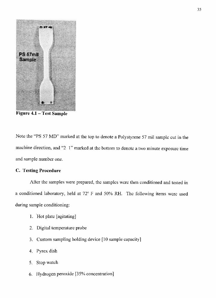
35
.-..:.
j-
W* rtf-
PS S7mil
Sample
Figure 4.1 - Test Sample
Note the "PS 57MD"
marked at the top to denote a Polystyrene 57 mil sample cut in the
machine direction, and "21"
marked at the bottom to denote a two minute exposure time
and sample number one.
C. Testing Procedure
After the samples were prepared, the samples were then conditioned and tested in
a conditioned laboratory, held at72
F and 50% RH. The following items were used
during sample conditioning:
1 . Hot plate [agitating]
2. Digital temperature probe
3. Custom sampling holding device [10 sample capacity]
4. Pyrex dish
5. Stop watch
6. Hydrogen peroxide [35% concentration]
36
7. Hydrogen peroxide concentration test kit, including the following:
Hydrometer tube
Thermometer
Hydrometer
Conversion charts
Hydrogen peroxide was first poured into the Pyrex dish, which was then placed on the
heating plate and heated. The digital temperature probe was placed into the H202 and
monitored. The H202 was then tested for concentration using the following procedure:
1 . Fill hydrometer tube with sample ofH202, approximately 500 ml.
2. Submerge thermometer into H202 in hydrometer tube.
3 . Record temperature [C] after reading has stabilized.
4. Submerge hydrometer into H202 in hydrometer tube, being careful not to allowthe hydrometer to contact the hydrometer tube.
5. Record specific gravity [g/cm3] from the bottom of the meniscus, after readinghas stabilized.
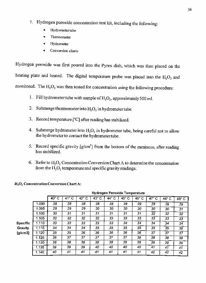
6. Refer to H202 ConcentrationConversion ChartA to determine the concentration
from the H202 temperature and specific gravity readings.
H,0, ConcentrationConversionChartA:
Hydrogen Peroxide Temperature
Specific
Gravity
[g/cm3]
40
C41
C42
C43
C44
C45
C46
C47
C48
C49
C
1.090 28 28 28 28 28 29 29 29 29 29
1.095 29 29 29 30 30 30 30 30 30 31
1.100 30 31 31 31 31 31 31 32 32 32
1.105 32 32 32 32 33 33 33 33 33 33
1.110 33 33 33 33 33 34 34 34 34 34
1.115 34 34 34 35 35 35 35 35 35 36
1.120 35 35 36 36 36 36 36 37 37 37
1.125 36 37 37 37 37 37 38 38 38 38
1.130 38 38 38 38 38 39 39 39 39 39
1.135 39 39 39 40 40 40 40 41 41 41
1.140 40 41 41 41 41 41 41 42 42 42

37
Hydrogen Peroxide Temperature
Specific
Gravity[g/cm3]
50
C51
C52
C53
C54
C55
C56
C57
C58
C59
C
1.090 30 30 30 30 30 30 30 31 31 31
1.095 31 31 31 31 31 32 32 32 32 32
1.100 32 32 32 33 33 33 33 33 33 34
1.105 33 34 34 34 34 34 34 34 35 35
1.110 35 35 35 35 35 35 36 36 36 36
1.115 36 36 36 36 36 37 37 37 37 37
1.120 37 37 37 38 38 j 38 38 38 38 38
1.125 38 38 39 39 39 39 39 40 40 40
1.130 40 40 40 40 40 41 41 41 41 41
1.135 41 41 42 42 42 42 42 42 43 43
1.140 42 43 43 43 43 43 43 44 44 44
Hydrogen Peroxide Temperature60
C 61C62
C63
C64
C65
C66
C67
C68
C69
C
1.090 31 31 31 32 32 32 32 32 32 33
1.095 32 33 33 33 33 33 33 34 34 34
1.100 34 34 34 34 34 34 35 35 35 35
1.105 35 35 35 35 36 36 36 36 36 36
Specific 1.110 36 36 37 37 37 37 37 37 38j
38
Gravity 1.115 37 38 38 38 38 38 38 39 39 39
[g/cm3] 1.120 39 39 39 39 39 40 40 40 40 40
1.125 40 40 41 41 41 41 41 42 42 42
1.130 42 42 42 42 42 42 43 43 43 43
1.135 43 43 43 43 43 44 44 44 44 45
1.140 44 44 45 45 45 45 45 46 46 46
After the concentration of H202 was verified to be within the required range of 34-36%,
and at the required temperature of55
C, the conditioning of samples began. Samples
were placed in a fixture designed to hold ten samples simultaneously, and placed in the
H202 bath. A stopwatch was used to monitor the time of exposure, and a digital
thermometer was used to monitor the bath temperature. After samples were given the
appropriate exposure, they were removed from the bath and placed on paper towels and
allowed to dry at ambient temperature, which was72
F / 50% RH. The samples were

38
then reconditioned, in the same manner as discussed previously, prior to testing. After
reconditioning was complete, the samples were tested on the following equipment:
Equipment: InstronModel 5500R (serial #1010)
Software: Instron Corporation Series IX AutomatedMaterialsTesting System
PS Testing Parameters: pp Testing Parameters:
Load Cell: 10001b. 10001b.
Crosshead Speed: 2 in./min. 5 in./min.
Grip Seperation: 2.5 in. 2.5 in.
The results were recorded through the use of the Instron software package and printed
out. These results were then analyzed usingMinitab
release 12 statistical software and
Microsoft
Excel 97 data analysis software.

39
in
on
Chapter 5
Results
In discussing the results of testing, the data must first be analyzed to determine its
relevance and whether conclusive results can be drawn from the data. The first step is to
determine the significance of the data variances within each sample set, and then i
relation to the total group of all sample sets. Therefore, an analysis will be performed
each material variable, and each subset within those variables, that will provide the
following statistical values:
1 . F-ratio, which is an analysis of variance ofmeans.
2. The coefficient of correlation, (r).
3. The coefficient ofdetermination, (r2).
A. Data Analysis
1. F-ratio
To begin, the null hypothesis is a method of analysis to determine the lack of
difference between two or more groups of data. The null hypothesis holds that there are
no significant differences between two or more groups of data, and certain tests, like F-
ratio, prove that the hypothesis either holds true or that it fails (Freund & Simon, 298).
The F-ratio is a statistical analysis of variance, which in the case of this thesis, will be
used to test the hypothesis that the data indicate there is no difference in the mechanical
properties of each material as it is exposed to increasing durations of heat and H202
(Freund & Simon, 394-396). So then, if null hypothesis holds true, then there is no

40
significant effect due to the increasing exposure to H202. Conversely, if the null
hypothesis is proven false, then there is enough statistical variation to indicate that the
alternative hypothesis is true, i.e., that exposure to H202 has an effect on the mechanical
properties of the test samples. So the comparison of the changes in one mechanical
property is only made within a group consisting of the ten samples of the same material
exposed to H202 for the seven varying durations of time.
The F-ratio must exceed a certain value for the null hypothesis to be rejected.
This value is determined using an algorithm and an F value table (Appendix F). First, the
F value that will be used as a comparison limit to either accept or reject the null
hypothesis is determined using the following equation:
Fo.os= (k- 1 ) / k (n- 1 ), when F0 05
= F factor @ 0.05 level of significance
k = # of sample sets (exposure times)= 7
n= # samples in each set = 10
Fo.os=
(7-1) / 7(10-1)= 6 / 63, and using Appendix F we find:
^0.05 2.2j
Then, the null hypothesis will be accepted if the F-ratio values are less than 2.25, and
rejected if they are greater than 2.25. When the F-ratio is very large, it is an indication
that the variation in mechanical properties due to the H202 exposure is much greater than
that due to random error. Conversely, when the F-ratio is very small it indicates that the
variations in mechanical properties can be attributed to random error or other unknown
variables. The actual F-ratio values are determined by the following equations (Freund &
Simon, 396):
Fratio= variation among sample set means / variation within samples (or)
41
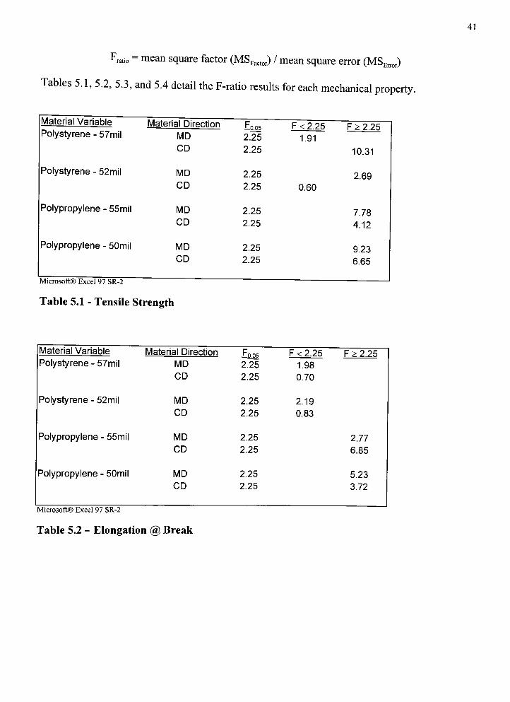
Frati0-
mean square factor (MSFactor) / mean square error (MSErior)
Tables 5.1, 5.2, 5.3, and 5.4 detail the F-ratio results for each mechanical property.
Material Variable Material Direction
MD
CD
E.0.05
2.25
2.25
F<2.25
1.91
F>2.25
10.31
Polystyrene - 57mil
Polystyrene - 52mil MD
CD
2.25
2.25 0.60
2.69
Polypropylene - 55mil MD
CD
2.25
2.25
7.78
4.12
Polypropylene - 50mil MD
CD
2.25
2.25
9.23
6.65
Table 5.1 - Tensile Strength
Material Variable Material Direction
MD
o.05
2.25
F<2.25
1.98
F>2.25
Polystyrene - 57mil
CD 2.25 0.70
Polystyrene - 52mil MD 2.25 2.19
CD 2.25 0.83
Polypropylene - 55mil MD 2.25 2.77
CD 2.25 6.85
Polypropylene - 50mil MD 2.25 5.23
CD 2.25 3.72
Microsoft Excel 97 SR-2
Table 5.2 - Elongation @ Break

42
Material Variable Material Direction
MD
CD
Eo.05
2.25
2.25
F<2.25
1.43
F>2.25
24.42
Polystyrene - 57mil
Polystyrene - 52mil MD
CD
2.25
2.25
2.15
0.30
Polypropylene - 55mil MD
CD
2.25
2.25
10.64
18.36
Polypropylene - 50mil
MicrninftrS) Fvrel 07 SO 1
MD
CD
2.25
2.25
7.42
9.99
Table 5.3 - Elongation @ Yield
Material Variable
Polystyrene - 57mil
Polystyrene - 52mil
Polypropylene - 55mil
Polypropylene - 50mil
Material Direction F005MD 2.25
CD 2.25
MD 2.25
CD 2.25
MD 2.25
CD 2.25
MD 2.25
CD 2.25
Microsoft Excel 97 SR-2
Table 5.4 - Modulus ofElasticity
F<2.25 F>2.25
3.24
4.18
2.49
0.62
5.65
4.17
10.78
5.39
2. Coefficient ofCorrelation
The next important statistical determinant is a measure of how well the dependant
variable, in this case the mechanical property of interest, relates to the independent
variable, duration of exposure to heat and H202. The coefficient of correlation, r, is used
in conjunction with a scatter plot diagram as a strong indicator of the linear relationship

43
canbetween two variables (Freund & Simon, 468 - 471). The coefficient of correlation
range from +1 to -1, inclusive. A value of +1 would indicate a perfect direct linear
correlation between the two variables, whereas a value of -1 would indicate a perfect
inverse linear correlation. A value of 0 (zero), on the other hand, would indicate that no
linear relationship exists between the two variables (Minitab, 4-5). The graphs in Figures
5.1, 5.2, and 5.3, below illustrate an example of each.
6
5
4
3
2
1
0
0
Direct Positive Linear Relationship(r=+1)
6
5
4
3
2
1
0
C
Direct Inverse Linear Relationship
(r=-1)
/*
\^X >^^
/*
^x^>\
12 3 4 5 6 12 3 4 5 6
6
5
4
3
2
1 -
0 -
C
No Linear Relationship
(r=0)
112 3 4 5 6
Figures 5.1, 5.2, 5.3. Examples ofPositive, Negative, and Zero Correlation Indications
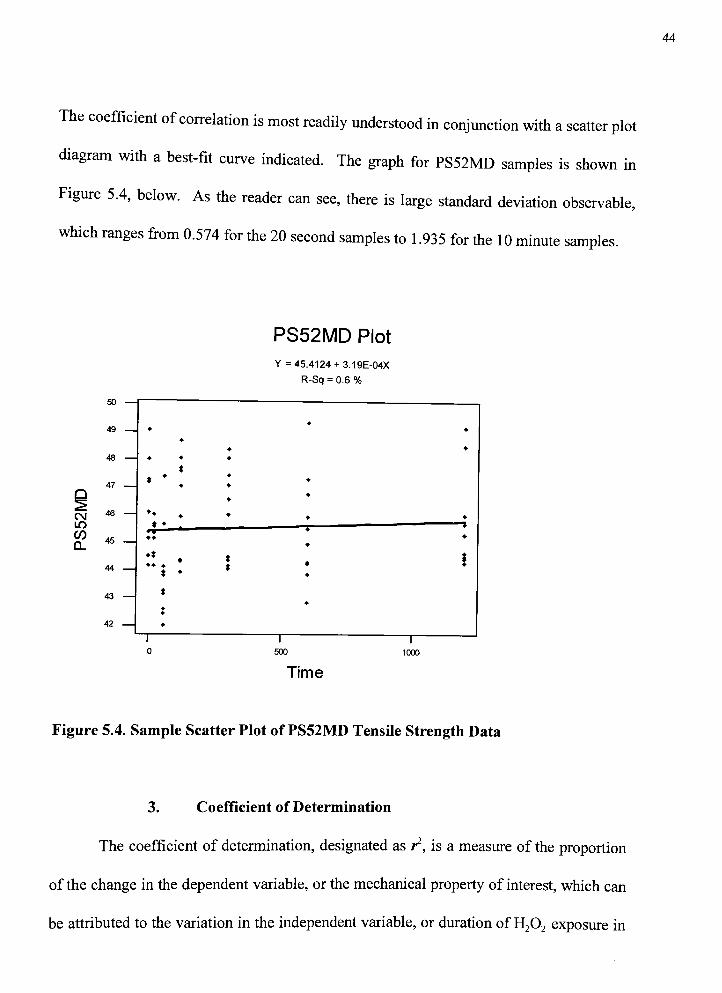
44
The coefficient of correlation is most readily understood in conjunction with a scatter plot
diagram with a best-fit curve indicated. The graph for PS52MD samples is shown in
Figure 5.4, below. As the reader can see, there is large standard deviation observable,
which ranges from 0.574 for the 20 second samples to 1 .935 for the 10 minute samplles.
PS52MD Plot
Y = 45.4124 + 3. 19E-04X
50
R-Sq = 0.6 %
?
49 ?
?
?
43 ?
**
?
t
?
*?
47 ___ ? ?
Q ?
^*
CMLO
CO
46? ?
? ?
45?? ?
Q_ ?
44
?*?? ?
$
t? !
43
t?
42 ?
1
0
1
500
I
1000
Time
Figure 5.4. Sample Scatter Plot ofPS52MD Tensile Strength Data
3. Coefficient ofDetermination
The coefficient of determination, designated as r2, is a measure of the proportion
of the change in the dependent variable, or the mechanical property of interest, which can
be attributed to the variation in the independent variable, or duration ofH202 exposure in

45
this case. The coefficient is expressed as a percentage and is equal to square of the value
of the coefficient of correlation, r, multiplied by 100 (Freund & Simon, 470). For
example, as indicated in the title block area ofFigure 4.4, above, the lvalue is calculated
to be 0.6%, indicating a very low variation in the mechanical property, tensile strength,
due to changes in the length of time the test samples were exposed to H202. The line fit
equation, Y= 45.41 + 3.19E-04 X, would support this conclusion (i.e., the tensile
strength would change by only 0.319 lbf for every thousand seconds of exposure). This
statistical measure, r2, therefore, has been selected as a dependable indication of the
relative strength of the relationship between the mechanical properties of interest and the
duration of exposure to H202 for the given periods of 0 (the control samples), 20, 60, 120,
300, 600, and 1200 seconds. The calculations for each material are listed in Tables 5.5,
5.6, 5.7 and 5.8.
Material Variable Material Direction r 1^(100)
0.5%
Linear Equation
y= 45.4 + 0.00031 9xPolystyrene - 52mil MD 0.074
CD -0.077 0.6% y= 34.8 - 0.000205X
Polystyrene - 57mil MD -0.048 0.2% y= 51.0-0.000182x
CD -0.321 10.3% y= 36.7-0.000314x
Polypropylene - 50mil MD -0.109 1.2% y= 64.6 -0.00041 5x
CD -0.428 18.3% y= 63.6-0.00126x
Polypropylene - 55mil MD -0.072 0.5% y= 73.0- 0.0001 95x
CD -0.284 8.1% y= 72.0-0.000668x
.
Minitab Statistical Software, release 12 for Windows 95/NT
Table 5.5 - Tensile Strength
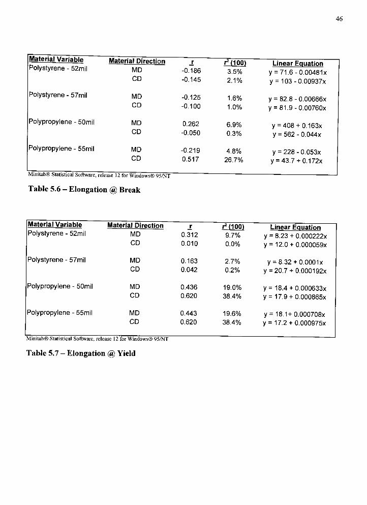
46
Material Variable Material Direction
MD
CD
-0.186
-0.145
HflOO)
3.5%
2.1%
Linear Equation
y= 71.6-0.00481x
y= 103-0.00937x
Polystyrene - 52mil
Polystyrene - 57mil MD
CD
-0.125
-0.100
1.6%
1.0%
y= 82.8 - 0.00666x
y= 81.9-0.00760x
Polypropylene - 50mil MD
CD
0.262
-0.050
6.9%
0.3%
y= 408 + 0.163x
y= 562 - 0.044x
Polypropylene - 55mil MD
CD
-0.219
0.517
4.8%
26.7%
y= 228 - 0.053x
y= 43.7 + 0.1 72x
Table 5.6 - Elongation @ Break
Material Variable
Polystyrene - 52mil
Polystyrene - 57mil
Polypropylene - 50mil
Polypropylene - 55mil
Material Direction r
MD 0.312
CD 0.010
MD 0.163
CD 0.042
MD 0.436
CD 0.620
MD 0.443
CD 0.620
Minitab Statistical Software, release 12 for Windows 95/NT
Table 5.7 - Elongation @ Yield
Hnoo Linear Eauation
9.7% y= 8.23 + 0.000222x
0.0% y= 12.0 + 0.000059x
2.7% y= 8.32 + 0.0001x
0.2% y= 20.7 + 0.0001 92x
19.0% y= 18.4 + 0.000633x
38.4% y= 17.9 + 0.000865x
19.6% y= 18.1+0.000708x
38.4% y= 17.2 + 0.000975x
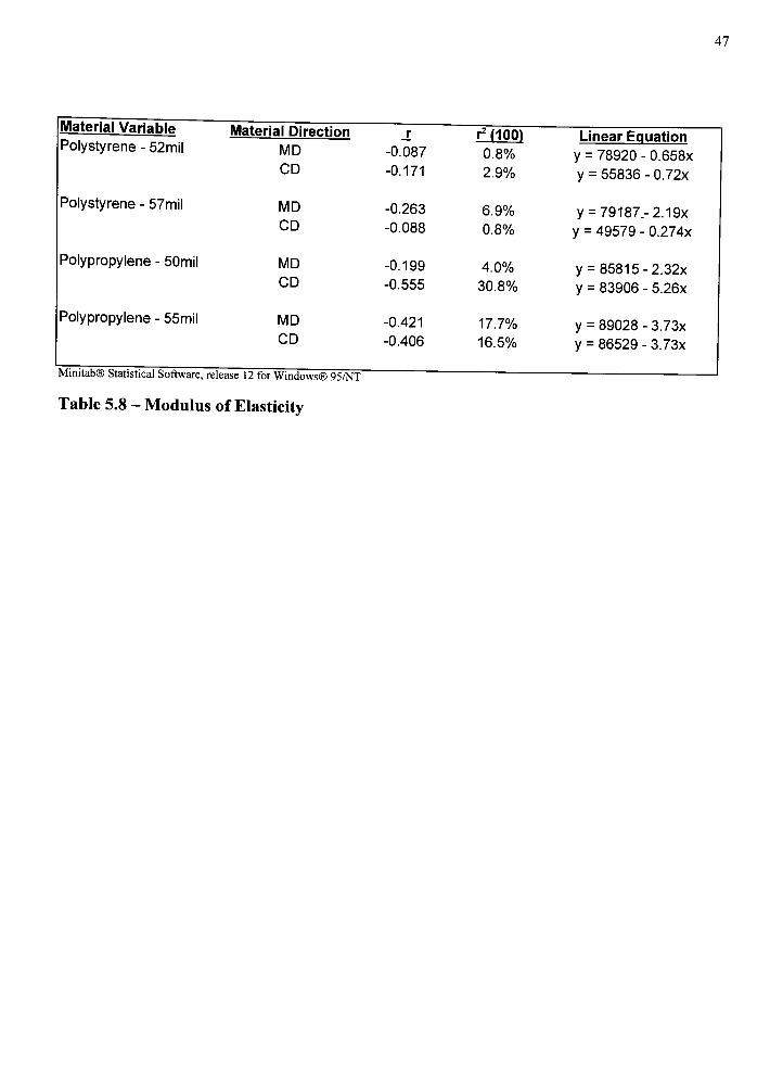
47
Material Variable Material Direction
MD
CD
-0.087
-0.171
1^(100.1
0.8%
2.9%
Linear Equation
y= 78920 - 0.658x
y= 55836 - 0.72x
Polystyrene - 52mil
Polystyrene - 57mil MD
CD
-0.263
-0.088
6.9%
0.8%
y= 79187_-2.19x
y= 49579 - 0.274x
Polypropylene - 50mil MD
CD
-0.199
-0.555
4.0%
30.8%
y= 85815 -2.32x
y= 83906 - 5.26x
Polypropylene - 55mil MD
CD
-0.421
-0.406
17.7%
16.5%
y= 89028 - 3.73x
y= 86529 - 3.73x
Table 5.8 - Modulus ofElasticity
48
Chapter 6
Conclusions & Recommendations
The approach taken in this section is to address each of the material variables
independently, then to integrate those findings to determine if a consistent relationship
exists. Each discussion will include a table with the relevant statistical data derived from
the testing results. This data will form the basis for the analysis and deductions.
A. Discussion ofResults
1. Polystyrene - 57 mil
For this material, the data was consistent for samples cut in the machine direction.
For three of the fourmechanical properties, the null hypothesis was accepted, which
indicates that there was no, or little, difference in the mechanical properties induced by
exposure to H202. For the one mechanical property, modulus of elasticity, in which the
null hypothesis was rejected, the coefficient of correlation, r, was slightly negative
showing a degrading effect. Further, the coefficient of determination, r2, indicated that a
very small proportion of the actual degradation was due to the H202 exposure. The linear
equation supports this, being a very flat line. See Table 6.1 below for data, and Appendix
for scatter plots and raw data. The conclusion, therefore, is that there is no statistically
significant degradation of the 57 mil polystyrene caused by any tested exposure to H202.

49
Polystyrene - 57mil
Machine Direction
Tensile Strength
Elongation @ Break
Elongation @ Yield
Modulus of Elasticity
Null Hypothesis f F )Accept (1.91) -0.048
Accept (1.98) -0.125
Accept (1.43) 0.163
Reject (3.24) -0.263
(accept if x < 2.25)
rMlOOl Linear Equation
0.2% y= 51.0- 0.0001 82x
1.6% y= 82.8 - 0.00666x
2.7% y= 8.32 + 0.0001x
6.9% y= 79187-2.19x
Polystyrene - 57mil
Cross Direction
Tensile Strength
Null Hvnothesis ( F )
Reject (10.31) -0.321
rMlOOl
10.3%
Linear Equation
y= 36.7 - 0.000314x
Elongation @ Break Accept (0.70) -0.100 1.0% y= 81.9-0.00760x
Elongation @ Yield Reject (24.42) 0.042 0.2% y= 20.7 + 0.000192x
Modulus of Elasticity Reject (4.18)
(accept if x < 2.25)
-0.088 0.8% y= 49579 - 0.274x
Table 6.1 - Polystyrene 57 mil
For the test samples cut in the cross direction, statistical indicators were slightly
more mixed. Although the null hypothesis was rejected for three of the four mechanical
properties, the r values remained low and the linear equations, again, yielded very flat
results. In fact, for the mechanical property, tensile strength, that exhibited the strongest
correlation statistically, the linear equation would predict a very minor change in that
property, e.g., less than 1% change over 1000 seconds of exposure. In addition, the
coefficient of determination, r2, indicates that only 10.3% of that variation should be
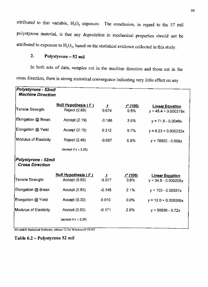
50
attributed to that variable, H202 exposure. The conclusion, in regard to the 57 mil
polystyrene material, is that any degradation in mechanical properties should not be
attributed to exposure to H202, based on the statistical evidence collected in this study.
2. Polystyrene - 52 mil
In both sets of data, samples cut in the machine direction and those cut in the
cross direction, there is strong statistical convergence indicating very little effect on any
Polystyrene - 52mil
Machine Direction
Tensile Strength
Elongation @ Break
Elongation @ Yield
Modulus of Elasticity
Polystyrene - 52mil
Cross Direction
Null Hvnothesis ( F )Reject (2.69) 0.074
rMlOO)
0.5%
Linear Equation
y= 45.4 + 0.00031 9x
Accept (2.19) -0.186 3.5% y= 71.6-0.0048x
Accept (2.15) 0.312 9.7% y= 8.23 + 0.000222x
Reject (2.49) -0.087 0.8% y= 78920 - 0.658x
(accept if x < 2.25)
Tensile Strength
Null Hvnothesis ( F )
Accept (0.60) -0.077
r2
dOO)
0.6%
Elongation @ Break Accept (0.83) -0.145 2.1%
Elongation @ Yield Accept (0.30) 0.010 0.0%
Modulus of Elasticity Accept (0.62)
(accept if x < 2.25)
-0.171 2.9%
Linear Equation
y= 34.8 - 0.000205X
y= 103-0.00937x
y= 12.0 + 0.000059X
y= 55836 - 0.72x
Minitab Statistical Software, release 12 for Windows 95/NT
Table 6.2 - Polystyrene 52 mil

51
of the mechanical properties of the test samples due to any tested duration of H202
exposure. For six of the eight sample groups, the null hypothesis was accepted, and the
coefficient of correlation also showed a negligible relationship, be it positive or negative.
The linear equations all predict a very small change in mechanical property for extended
periods of exposure to H202. And the coefficient of determination indicates that any
changes that would occur are more likely to be caused by other factors. Table 6.2
summarizes the statistical indicators to support this assertion.
3. Polypropylene - 55 mil
Prior to discussing the results of the statistical indicators previously used to
determine the relationship between H202 exposure duration and degradation of
mechanical properties, it is necessary to address the validity of the data. A study of the
elongation at break data has suggested that the data may not be statistically valid due to
large standard deviations. Specifically, the standard deviations for the 55 mil
polypropylene averaged 86% of the average (elongation at break) value for samples cut in
the cross direction and 40% for the samples cut in the machine direction. In addition, a
review of the scatter plots for these measurements support the exclusion of this data as a
source ofdegradation prediction.
For all test groups the null hypothesis was rejected, indicating that there was a
difference in the mechanical properties after exposure to H202. This leads to further
investigation into what type of difference would be expected, and to what degree the
exposure to H202 contributed to the change. In this case, the coefficient of correlation is
consistent among all three usable indicators, tensile strength, elongation at yield, and
modulus of elasticity. Tensile strength and modulus of elasticity predictors show that as

52
the exposure duration increases, there will be a decrease in those properties. Conversely,
elongation at yield has a positive relationship, with the predictors showing that this
property would increase as exposure duration increases. These results are consistent in
the physical manifestation of the plastic's properties, i.e., as the tensile strength decreases
and the elongation at yield increases, it would cause the modulus of elasticity to decrease.
The modulus of elasticity is equal to stress divided by strain, which reduces to force
divided by elongation, when gauge length and cross section area are held constant. Given
that, the tensile strength is decreasing and elongation at yield is increasing, the modulus
should decrease, which it does. These factors all point to increasing elasticity as a
function of increased exposure, with coefficient ofdetermination values ranging from less
than one percent to 38%. A study of the raw data however, shows that the values tend to
change in a non-linear manner, which is consistent with plastics (ASTM D 638-94b, note
A2.3). This result would indicate that the exposure to H202 is not creating the problems
that led to this study. Refer to Table 6.3 for statistical reference data and Appendix A for
scatter plots and Appendix B for the raw data.
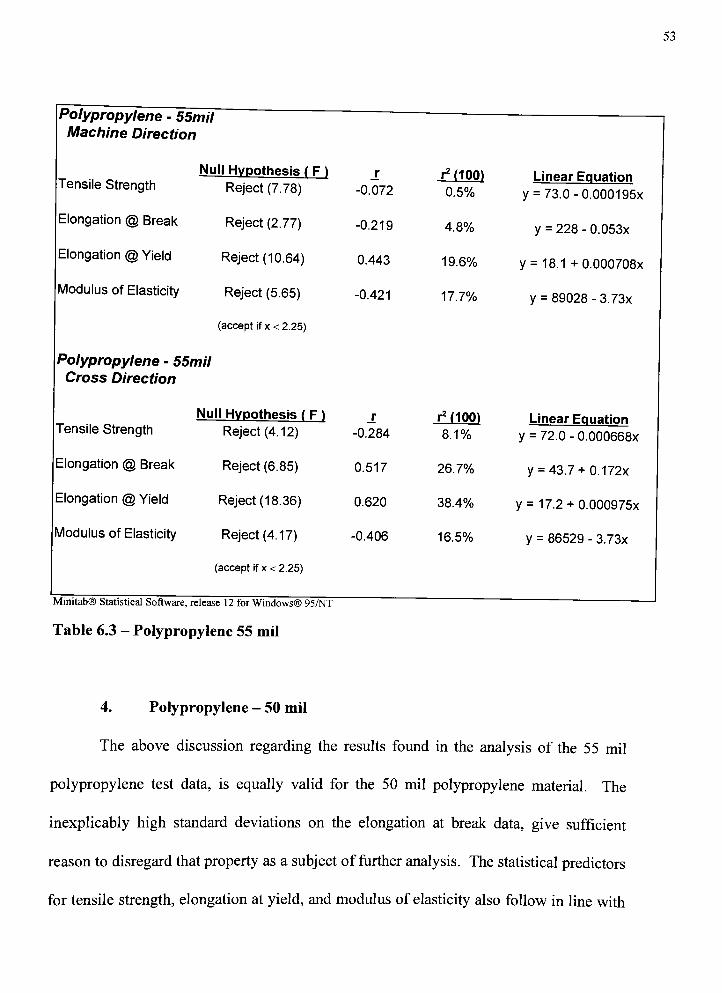
53
Polypropylene - 55mil
Machine Direction
Tensile Strength
Elongation @ Break
Elongation @ Yield
Modulus of Elasticity
Null Hypothesis ( F )
Reject (7.78)
Reject (2.77)
Reject (10.64)
Reject (5.65)
(accept if x < 2.25)
Polypropylene - 55mil
Cross Direction
Tensile Strength
Elongation @ Break
Elongation @ Yield
Modulus of Elasticity
Null Hypothesis ( F )Reject (4.12)
Reject (6.85)
Reject (18.36)
Reject (4.17)
(accept if x< 2.25)
Minitab Statistical Software, release 12 for Windows 95/NT
Table 6.3 - Polypropylene 55 mil
-0.072
-0.219
0.443
-0.421
-0.284
0.517
0.620
-0.406
i^dOOl
0.5%
4.8%
19.6%
17.7%
r'dOO)
8.1%
26.7%
38.4%
16.5%
Linear Equation
y= 73.0- 0.0001 95x
y= 228 - 0.053x
y= 18.1 +0.000708X
y= 89028 - 3.73x
Linear Equation
y= 72.0 - 0.000668X
y= 43.7 + 0.172x
y= 17.2 + 0.000975x
y= 86529 - 3.73x
4. Polypropylene - 50 mil
The above discussion regarding the results found in the analysis of the 55 mil
polypropylene test data, is equally valid for the 50 mil polypropylene material. The
inexplicably high standard deviations on the elongation at break data, give sufficient
reason to disregard that property as a subject of further analysis. The statistical predictors
for tensile strength, elongation at yield, and modulus of elasticity also follow in line with

54
the results for the 55 mil material. The results of the analysis, therefore, are identical.
Use Table 6.4 as a comparison of the statistical results for the 50 mil polypropylene
material.
Polypropylene - 50miI
Machine Direction
Tensile Strength
Elongation @ Break
Elongation @ Yield
Modulus of Elasticity
Null Hypothesis ( F )Reject (9.23)
Reject (5.23)
Reject (7.42)
Reject (10.78)
(accept if x < 2.25)
Polypropylene - 50miI
Cross Direction
Tensile Strength
Null Hypothesis ( F )
Reject (6.65)
-0.109
0.262
0.436
-0.199
-0.428
Minitab Statistical Software, release 12 for Windows 95/NT
Table 6.4 - Polypropylene 50 mil
rMlOO)
1.2%
6.9%
19.0%
4.0%
r2
dOO)
18.3%
Elongation @ Break Reject (3.72) -0.050 0.3%
Elongation @ Yield Reject (9.99) 0.620 38.4%
Modulus of Elasticity Reject (5.39)
(accept if x < 2.25)
-0.555 30.8%
Linear Equation
y= 64.6- 0.00041 5x
y= 408 + 0.163x
y= 18.4 + 0.000633x
y= 85815 -2.32x
Linear Equation
y= 63.6-0.00126x
y= 562 - 0.044x
y= 17.9 + 0.000865x
y= 83906 - 5.26x
5. Scanning Electron Microscope (SEM) Photographs
A sample each of the polystyrene and polypropylenematerials was subjected to an
examination by a SEM at a magnification of 10,000x, with photographs taken to
55
document the results. A comparison of samples subjected to H202 for test periods of zero
time and twenty minutes provided an indication that no degradation to the surface of the
materials was occurring. This would support the deduction that since no physical change
was observable, no change in mechanical properties would be expected. See Appendix D
for SEM photographs.
In conclusion, testing performed on the polystyrene and polypropylene materials
did not support the original hypothesis that increased exposure to H202 would degrade the
mechanical properties of those materials. Nor was there any indication that as the
materials thickness was reduced, there would be an increased propensity to degrade due
to an increased exposure to H202.
The polystyrene material exhibited very little, or no, change in mechanical
properties that could be attributed to the exposure to H202. This would indicate that
variations were based more on other factors, such as material impurities, differences in
material characteristics due to variations in the extrusion process, imprecision in testing
procedures, etc. One is lead to the conclusion, therefore, that the issues that led to this
research project, i.e., increased brittleness leading to web and edge strip breaks in the
aseptic process, can not be attributed to an increase in H202 exposure.
The polypropylene material, alternatively, did exhibit some relation between
material properties and exposure to H202. Both the 50 and 55 mil materials demonstrated
consistent trends in terms of the physical property changes. These changes, however,
were not negligible, but very small and left significant doubt as to their negative impact
in the aseptic process.

56
B. Recommendations for Further Study
As described in the statement of the problem in Chapter 3, the cup stock material
was becoming brittle when machine stoppages caused it to be trapped motionless in the
hydrogen peroxide bath. Initially, it was widely assumed that the cause of the problem
lay in the increased exposure to H202. As a result of the findings of this study, a further
examination of the possible causes of the observed increase in material brittleness during
the aseptic process was completed. Other potential causes of the degradation in the
mechanical properties of the material included heat, tension, and stress due to curvature
around a roller. It was found that the maximum amount of degradation occurred in
locations in contact with the rollers. Further lab testing was performed to corroborate this
observation and it was proven correct. The problem has been resolved by increasing the
diameter of the roller and thereby reducing the stress gradient resulting from the small
radius of the original rollers.
Although the problem has been resolved with empirical testing and trial and error
corrective action, it would be useful to follow up with a more formal investigation and
sensitivity analysis to establish the significance of each of the aforementioned factors. In
this way, mechanical design guidelines for future packaging equipment could be
established.
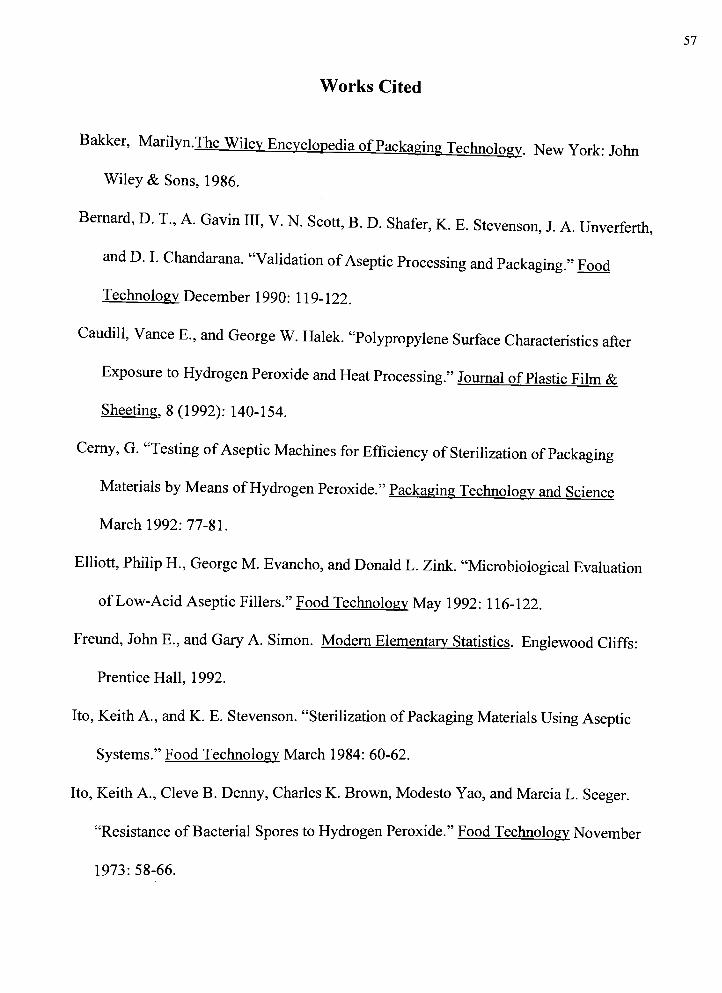
57
Works Cited
Bakker, Marilyn.The Wiley Encyclopedia ofPackaging T__hnology New York: John
Wiley & Sons, 1986.
Bernard, D. T., A. Gavin III, V. N. Scott, B. D. Shafer, K. E. Stevenson, J. A. Unverferth,
and D. I. Chandarana. "Validation ofAseptic Processing andPackaging."
Food
Technology December 1990: 119-122.
Caudill, Vance E., and George W. Halek. "Polypropylene Surface Characteristics after
Exposure to Hydrogen Peroxide and HeatProcessing."
Journal ofPlastic Film &
Sheeting. 8 (1992): 140-154.
Cerny, G. "Testing ofAseptic Machines for Efficiency of Sterilization ofPackaging
Materials by Means ofHydrogenPeroxide."
Packaging Technology and Science
March 1992: 77-81.
Elliott, Philip H., George M. Evancho, and Donald L. Zink. "Microbiological Evaluation
ofLow-Acid AsepticFillers."
Food Technology May 1992: 1 16-122.
Freund, John E., and Gary A. Simon. Modern Elementary Statistics. Englewood Cliffs:
Prentice Hall, 1992.
Ito, Keith A., and K. E. Stevenson. "Sterilization ofPackaging Materials Using Aseptic
Systems."
Food Technology March 1984: 60-62.
Ito, Keith A., Cleve B. Denny, Charles K. Brown, Modesto Yao, andMarcia L. Seeger.
"Resistance ofBacterial Spores to HydrogenPeroxide."
Food Technology November
1973: 58-66.

58
Komerska, Jim. Constraints Imposed bv Sterilization Method on Selection ofPackaging
Materials- 1991 Polymers, Laminations & Coatings Conference, Sept. 3-6, 1991,
San Diego. Atlanta: Tappi Press, 1991.
Mans, J. "Showcase: Aseptic Packaging." Prep. Foods 157.3 (1988): 106.
MeetMinitab: Release 12 forWindows
State College: Minitab Inc., 1997.
Newsome, Rasetta L. ed. "Perspective on Food Irradiation." Food Technology. February
1987. pp. 100-101.
Ogorkiewicz, R. M. Thermoplastics: Effects ofProcessinp Cleveland: The Chemical
Rubber Co., 1969.
Paine, F. A. The Packaging User's Handbook New York: Chapman & Hall USA, 1995.
Radiation Sterilizers Incorporated. RSI Gammagram. Illinois: Radiation Sterilizers
Incorporated, 1988.
Reuter, H. Aseptic Packaging ofFood. Lancaster: Technomic Publishing Company,
Inc., 1989.
Robertson, Gordon L. Food Packaging: Principles and Practice. New York: Marcel
Dekker, Inc., 1993.
Storer, Roberta, ed. 1995 Annual Book ofASTM Standards. 08.01:47-58 Easton: 1995.
Strupinsky, Gene, and Aaron L. Brody. A Twenty-Year Retrospective on Plastics:
Oxygen Barrier Packaging Materials. 1988 Polymers, Laminations & Coatings
Conference, Aug. 30 - Sept. 3, 1988, San Francisco. Atlanta: Tappi Press, 1998.
Yambrach, Fritz. "Modified Atmosphere Packaging ofSea-foods."
Journal ofPackaging
Technology 1.5 (1987): 154

Tensile Strength Scatter-Plots
Appendix A
59
PS52MD Plot
Y- 45.4124 + 119E-04X
50
R-Sq -08%
40.
*
?
a
46
47 -
t'
.246
45
44<
.
10
WQ-
t?
1
43
t
42
0 SCO
I
woo
Time
PS57MD Plot
Y .51.0182 -1.62E-04X
R-Sq - 0.2 S
545
.
*
5X5
.
525 .t
fe51.5
515
-
<6
.
t
Q.
?.
405 -<
.
t* *
t
4S.5 . t *
i i
PS52CD Plot
Y- 34.8164 -Z06E-04X
R-Sq - 0.6%
37
*
36 __
<4 .t
. .t
n?
oCM
35 -
.
CO*
0_
?
*
: .
34
*
*
:
t
t
t 1
t
33
I 1 1
Time
PS57CD Plot
Y" 36.7346 -3.14E-04X
R-Sq- 103%
375
?
*
t
37.0 *
ao
- t .
i*o 1 1*
CO 38.5
a.
38.0
*
1
?
4 t
i 1 '
TimeTime
a
soio
0La.
67
60
5
64
es
62
61
__L
PP50MD Plot
Y.M.eon.4.ise^Kx
R-Sq-1.2%
Time
1000
06
< t
64
n"?t-
oo
S3
10 ,
n.
D. 62
PP50CD Plot
Y' 63 5854- 1.26E-03X
R~Sq- 18.3%
I
500
I
WOO
Time

60
PP55MD Plot
Y-72.MM-1.KE-04X
R-Sq - 0.5 S
7J5.
n&
.?
a
74.5i
*
*
* t
?
10m
CL
73S
725 f
?
?1
LL.
? 1*
71.S1 *
*
'
705
Time
PP55CD Plot
y7i
2-e.eae-04x
R-Sq.8.1%
I
1000
Time
Elongation @ Break Scatter-Plnts
PS52MD Plot
Y- 715640- 4.S1E-03X
R-Sq15%
OOCM
lO
w0-
PS52CD Plot
Y 103221 -BJ7E-C3X
R-Sq > 21%
Time Time
PS57MD Plot PS57CD Plot
Y. 62.7562 -6.66E-0K
R-Sq>1.6K
Y.61.9355-7.60E-O3X
R-Sq1.0%
IO
ff
150
*
100
V?
*
?
*
1.
_
1 t ?
**
**
*?
50 l
-i l '
?
150
*
QOr-
COa.
103?
** *
? *
*
*
*
*
,
SO6*
i
i
1 I i'
Time Time

61
D
5o
Q.
PP50MD Plot
Y" 407.707? 0.162S6SX
R-Sq* 8.9%
WOO ?
, 1900
800 '<
700 ? '
800
600* ?
1
*
400
300
200
t
?
t
t *
100
0
1r~
1000
Time
a
if)
Q.0-
PP50CD Plot
Y- 561.737 -4.35E-02X
R-Sq - 0.3 %
Time
m 400
m #
n
n.?
. <
200
.t
PP55MD Plot
Y- 236.494 -S.30E-OW
R-Sq. 4.8%
I
1000
DOinlO
0.0.
PP55CD Plot
Y 43.6999+ Q.171640X
R-Sq2BJ%
700
800
4>
500
400
.
300
*
'
6>
200 * *
^
100
16
0
I 1 |
Time Time
Elongation (a). Yield Scatter-PIots
PS52MD Plot PS52CD Plot
Y-\23133222-0
R-Sq* 8.7%
Y- 11.8721 + 5.87E-OSX
R-Sq > 0.0%
QOojin
OTQ.
17
18
IS?
14?
* i > 1 J*
13
12
?*
?
,
11
10 *
9
," ?
*
i i
r
1000
Time Time

62
PS57MD Plot PS57CD Plot
Y" 631850 4 1.0OC-O4X
R-Sq- 26%
Y> 206656. 1.82E-04X
R-Sq. 02%
QOr- *
in
w0.
18
17
4
1
1 1
t
0
* 1
1 1 I
Time Time
PP50MD Plot PP50CD Plot
Y. 164264. 6L-04X
R-Sq- 18.0%
Y 17.8373 + aeSC-CKX
R-Sq. 36.4%
Oin
o_0-
195 *
?+
+
:
+
?
ws
+
?
175
+
1 1 1
QOom
CL0.
?
195?
+
* ?
185 ?
?
* ? ?
+
+ *
? *
**
175
1 1 1
Time Time
PP55MD Plot PP55MCD Plot
Y 18.1216 + 7.06E-04X
R-Sq* 19.6%
Y* 17.1963+ 9.75E-04X
R-Sq=305%
165?
%*
IOm
nCL X
Time
- r
1000
Time

Modulus ofElasticity Scatter-Plnts
63
Q
2CMin
CO0.
PS52MD Plot
Y.7S320.3. 0.8570931
R-Sq. 07*
PS52CD Plot
Y. 55535.6- 0720147X
R-Sq. 28%
TimeTime
in
2
PS57MD Plot
Y-78187.4-2.1S541X
R-Sq - C.i %
o
O
CO0.
PS57CD Plot
Y- 49579.0 -0-~O2SX
R-Sq * as%
#
52000
:
51000+
U
*
*t.
<
50000
*
?
<
.
*
?
i
46000
*
?*
47000
*
t
i i
Time Time
PP50MD Plot PP50CD Plot
Y* 656145- Z31G62X
R-Sq 4.0%
Y* 83905.7 -&2S937X
R-Sq - 30.6 %
O
Q.
Time Time

64
Q
2
Q.
PP55MD Plot
Y. 690262 .J.73075X
R-Sq. 17.6%
Time
1
I**
*
n *
o ? 1in 65000 .
m
nQ_ { t
PP55CD Plot
Y-B95269-&73009X
R-Sq 165 %
-~r~
1000
Time
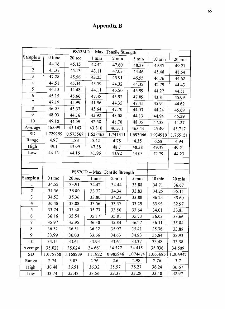
Appendix B
65
PS52MD - Max. Tensile Strength
Sample # 0 time 20 sec 1 min 2 min 5 min 10 min 20 min
1 44.16 45.15 42.42 47.60 48.38 49.37 49.21
2 45.37 45.13 43.11 47.03 44.46 45.48 48.54
3 47.28 45.56 43.25 45.91 46.55 46.76 44.62
4 44.51 45.34 43.79 44.32 44.35 42.79 44.43
5 44.13 44.48 44.11 45.50 45.99 44.27 44.51
6 45.15 45.66 47.38 43.92 47.09 43.81 45.99
7 47.19 45.99 41.96 44.35 47.41 45.91 44.62
8 46.07 45.37 45.64 47.70 44.03 44.24 45.69
9 48.03 44.16 43.92 48.08 44.13 44.94 45.29
10 49.10 44.59 42.58 48.70 48.05 47.33 44.27
Average 46.099 45.143 43.816 46.311 46.044 45.49 45.717
SD 1.729299 0.573567 1.628463 1.741311 1.693066 1.934919 1.765151
Range 4.97 1.83 5.42 4.78 4.35 6.58 4.94
High 49.1 45.99 47.38 48.7 48.38 49.37 49.21
Low 44.13 44.16 41.96 43.92 44.03 42.79 44.27
PS52CD - Max. Tensile Strength
Sample # 0 time 20 sec 1 min 2 min 5 min 10 min 20 min
1 34.52 33.91 34.42 34.44 33.88 34.71 36.67
2 34.36 36.00 33.72 34.34 33.83 34.25 35.11
3 34.52 35.36 33.80 34.23 33.80 36.24 35.60
4 36.48 33.88 33.56 33.37 33.29 33.93 32.97
5 33.74 33.48 35.73 33.50 33.64 34.01 33.85
6 36.16 35.54 35.17 35.81 35.73 36.03 33.66
7 35.97 35.95 36.30 35.84 36.27 36.11 35.84
8 36.32 36.51 36.32 35.97 35.41 35.76 33.88
9 33.99 36.00 33.66 34.63 34.93 35.84 33.93
10 34.15 33.61 33.93 33.64 33.37 33.48 33.58
Average 35.021 35.024 34.661 34.577 34.415 35.036 34.509
SD 1.075768 1.168239 1.11922 0.985946 1.074474 1.063685 1.206947
Range 2.74 3.03 2.76 2.6 2.98 2.76 3.7
High 36.48 36.51 36.32 35.97 36.27 36.24 36.67
Low 33.74 33.48 33.56 33.37 33.29 33.48 32.97

66
PS57MD - Max. Tensile Strength
Sample # 0 time 20 sec 1 min 2 min 5 min 10 min 20 min
1 52.89 50.36 51.68 50.36 51.79 53.99 51.03
2 53.34 52.62 51.14 51.01 52.38 48.86 52.51
3 51.30 49.02 50.28 54.36 51.73 51.73 53.32
4 51.95 49.99 52.48 51.65 51.14 49.32 52.83
5 51.87 51.03 49.93 53.18 49.34 50.50 49.72
6 50.42 49.58 51.36 54.28 48.54 48.81 51.41
7 50.09 49.64 53.07 51.89 49.18 49.56 49.93
8 54.04 50.55 50.76 51.03 48.46 48.72 50.36
9 51.70 52.21 49.13 49.10 51.60 48.51 50.79
10 48.46 52.13 51.36 49.42 49.18 49.21 51.97
Average 51.606 50.713 51.119 51.628 50.334 49.921 51.387
SD 1.648988 1.24549 1.168698 1.843552 1.523484 1.730603 1.240995
Range 5.58 3.6 3.94 5.26 3.92 5.48 3.6
High 54.04 52.62 53.07 54.36 52.38 53.99 53.32
Low 48.46 49.02 49.13 49.1 48.46 48.51 49.72
PS57CD - Max. Tensile Strength
Sample # 0 time 20 sec 1 min 2 min 5 min 10 min 20 min
1 37.58 36.72 37.37 36.11 37.18 37.37 36.67
2 37.34 36.75 36.19 36.91 37.15 36.78 36.24
3 37.23 36.59 36.30 36.91 36.86 37.10 35.95
4 36.75 36.24 36.83 36.56 36.59 36.89 36.35
5 37.07 36.56 36.56 36.64 36.78 36.78 36.03
6 36.99 36.13 37.10 36.32 36.70 36.78 36.03
7 36.91 36.38 36.13 36.48 36.67 37.32 36.27
8 36.91 36.32 35.76 36.40 36.97 36.59 36.05
9 36.86 36.32 36.59 36.40 36.81 36.67 36.24
10 36.78 36.32 36.27 36.56 37.05 36.24 35.95
Average 37.042 36.433 36.51 36.529 36.876 36.852 36.178
SD 0.26645 0.209181 0.484195 0.24933 0.204298 0.340287 0.224093
Range 0.83 0.62 1.61 0.8 0.59 1.13 0.72
High 37.58 36.75 37.37 36.91 37.18 37.37 36.67
Low 36.75 36.13 35.76 36.11 36.59 36.24 35.95

67
PP50MD - Max. Tensile Strength
Sample # 0 time 20 sec 1 min 2 min 5 min 10 min 20 min
1 63.01 66.93 66.58 64.75 63.79 63.54 65.88
2 64.97 66.44 67.36 63.65 65.05 62.28 64.89
3 64.43 64.38 66.93 64.81 63.60 63.68 65.91
4 63.44 64.78 63.17 65.07 63.65 63.62 63.65
5 63.87 65.21 64.56 64.67 63.57 63.11 62.42
6 62.66 67.36 64.00 63.97 64.62 62.98 64.13
7 63.38 68.24 64.19 67.11 65.61 63.09 64.30
8 61.74 67.52 62.55 66.34 65.40 63.33 64.78
9 61.53 66.36 63.25 66.60 65.37 62.87 64.43
10 60.91 65.07 63.25 65.64 64.38 62.28 66.07
Average 62.994 66.229 64.584 65.261 64.504 63.078 64.646
SD 1.301821 1.309923 1.744402 1.136852 0.818647 0.501194 1.135559
Range 4.06 3.86 4.81 3.46 2.04 1.4 3.65
High 64.97 68.24 67.36 67.11 65.61 63.68 66.07
Low 60.91 64.38 62.55 63.65 63.57 62.28 62.42
PP50CD - Max. Tensile Strength
Sample # 0 time 20 sec 1 min 2 min 5 min 10 min 20 min
1 63.54 65.56 64.64 65.32 64.56 64.03 64.13
2 63.17 64.11 62.17 63.49 62.63 60.54 64.00
3 62.93 64.99 64.27 63.11 63.25 61.50 62.23
4 62.52 65.18 62.44 62.90 63.44 62.68 62.87
5 62.93 65.10 63.36 62.95 63.19 61.58 63.17
6 63.22 63.92 62.20 61.50 63.97 61.61 62.42
7 63.95 64.38 64.38 63.54 62.42 60.91 62.39
8 64.81 64.27 63.57 62.07 63.46 63.06 60.83
9 65.40 63.89 62.98 62.07 63.62 62.63 59.92
10 64.86 63.44 62.63 62.12 62.23 61.74 63.09
Average 63.733 64.484 63.264 62.907 63.277 62.028 62.505
SD 0.979479 0.685974 0.927616 1.085583 0.711931 1.057343 1.307128
Range 2.88 2.12 2.47 3.82 2.33 3.49 4.21
High 65.4 65.56 64.64 65.32 64.56 64.03 64.13
Low 62.52 63.44 62.17 61.5 62.23 60.54 59.92

68
PP55MD - Max. Tensile Strength
Sample # 0 time 20 sec 1 min 2 min 5 min 10 min 20 min
1 72.89 76.32 73.40 72.59 71.62 72.46 74.34
2 72.08 74.07 73.88 74.36 72.19 71.95 73.23
3 71.70 74.71 71.68 73.40 72.48 73.21 71.87
4 71.65 74.58 73.77 73.26 75.17 73.05 72.19
5 72.56 73.61 74.36 72.16 73.64 72.05 74.09
6 72.75 73.83 72.05 71.14 73.21 73.37 72.08
7 72.48 73.83 71.95 70.60 72.91 72.59 72.75
8 71.89 75.22 71.60 71.41 73.29 72.78 72.38
9 72.51 74.25 72.00 72.13 73.13 72.83 74.09
10 72.67 75.09 72.38 71.57 73.61 72.03 71.84
Average 72.318 74.551 72.707 72.262 73.125 72.632 72.886
SD 0.4506 0.826014 1.033345 1.157294 0.961391 0.50686 0.981305
Range 1.24 2.71 2.76 3.76 3.55 1.42 2.5
High 72.89 76.32 74.36 74.36 75.17 73.37 74.34
Low 71.65 73.61 71.6 70.6 71.62 71.95 71.84
PP55CD - Max. Tensile Strength
Sample # 0 time 20 sec 1 min 2 min 5 min 10 min 20 min
1 74.55 71.01 71.79 73.45 73.72 72.19 72.70
2 73.77 71.84 71.81 72.46 72.86 71.70 71.46
3 72.56 71.92 71.14 71.87 72.78 71.22 71.01
4 73.15 71.95 71.81 71.89 72.70 71.19 71.01
5 72.81 71.84 72.30 71.84 72.32 71.46 71.09
6 72.19 72.48 70.25 71.87 71.73 72.83 71.03
7 71.62 71.68 70.58 71.38 71.62 72.78 70.63
8 71.46 71.14 71.22 72.48 70.95 72.27 70.63
9 71.46 70.28 71.14 72.64 70.42 71.95 69.74
10 71.41 70.58 70.60 73.13 69.48 71.52 70.55
Average 72.498 71.472 71.264 72.301 71.858 71.911 70.985
SD 1.083172 0.691179 0.659616 0.64815 1.285118 0.596852 0.758101
Range 3.14 2.2 2.05 2.07 4.24 1.64 2.96
High 74.55 72.48 72.3 73.45 73.72 72.83 72.7
Low 71.41 70.28i
70.25 71.38 69.48 71.19 69.74

69
PS52MD ~ % Elongation @ Break
Sample # Otime 20 sec 1 min 2 min 5 min 10 min 20 min
1 89.3 74.1 77.3 78.7 93.3 77.6 90.7
2 85.9 59.7 83.8 72.8 78.8 80.4 55.5
3 61.5 65.3 62.7 81 69.6 76.9 65.3
4 66.1 64.3 78 57 68.4 67.6 68.7
5 69.3 55.9 79.7 67.3 78.7 53 55.5
6 68.7 58.3 83.2 64.5 70.9 71.6 71.6
7 81.1 62.1 79.9 68.1 60.8 54.7 70.8
8 67.1 82.7 80.7 57 74.7 71.3 65.5
9 84.2 76 80.1 68.1 54.9 58.4 48.5
10 59.6 46.1 64.4 65.5 86.1 71.9 60.1
Average 73.28 64.45 76.98 68 73.62 68.34 65.22
SD 10.79494 10.72932 7.363695 7.941033 11.36494 9.759576 11.68092
Range 29.7 36.6 21.1 24 38.4 27.4 42.2
High 89.3 82.7 83.8 81 93.3 80.4 90.7
Low 59.6 46.1 62.7 57 54.9 53 48.5
PS52C D % Elongation @ Break
Sample # Otime 20 sec 1 min 2 min 5 min 10 min 20 min
1 103.7 123.5 98.1 110 112.3 96.4 75.4
2 82.6 109 79.5 134.8 117.7 111.1 96.3
3 97.7 97.8 134.6 147.1 138 141.1 94.8
4 154.8 140.2 72.3 106.8 99.5 150.5 52.6
5 70.4 104.5 109.1 75.1 68.8 80 53.1
6 90.1 72.1 73.3 122.8 135.9 35 85.4
7 106.9 71.9 100.6 64.4 83.1 66.4 116.5
8 130.2 78.5 112.4 106.9 97.2 117.6 91
9 72.4 113.3 104.4 63.3 105.1 144.8 119.6
10 100.4 86 95.7 91.4 100.4 149.9 66
Average 100.92 99.68 98 102.26 105.8 109.28 85.07
SD 25.84582 22.79502 19.25265 28.67497 21.48462 39.54634 23.49889
Range 84.4 68.3 62.3 83.8 69.2 115.5 67
High 154.8 140.2 134.6 147.1 138 150.5 119.6
Low 70.4 71.9 72.3 63.3 68.8 35 52.6

70
PS57MD - % Elongation @ Break
Sample # Otime 20 sec 1 min 2 min 5 min 10 min 20 min
1 101.7 111.1 96.2 92.2 92.3 77.1 104.3
2 108.9 56.3 148.7 115.3 84 63 53.8
3 100.7 72.8 82.7 72.3 69.5 49.4 44.6
4 122 71.9 66.5 57.6 74.6 82.4 48.9
5 90.9 61.1 100.8 41.2 64.7 47.7 78.5
6 58.2 66.5 71 61.6 86.6 84.5 66.8
7 111.4 83.2 92.5 89.5 98.9 66.2 83.1
8 51.7 76.6 75.4 101.2 100.5 96.3 127.5
9 94.6 48 86.5 61 102.8 71.4 99.7
10 105.9 50.2 66.6 78.3 78.6 66.8 74.5
Average 94.6 69.77 88.69 77.02 85.25 70.48 78.17
SD 22.68592 18.47858 24.33418 22.644 13.36656 15.27924 26.50891
Range 70.3 63.1 82.2 74.1 38.1 48.6 82.9
High 122 111.1 148.7 115.3 102.8 96.3 127.5
Low 51.7 48 66.5 41.2 64.7 47.7 44.6
PS57CD % Elongation @ Break
Sample # Otime 20 sec 1 min 2 min 5 min 10 min 20 min
1 56 69.4 103 79.7 164.4 68.2 73.5
2 148 83.7 80.5 87.2 55.3 52.9 68.7
3 148.7 84 86.1 42 92.8 68.6 60.6
4 59.9 54.4 42.9 37.9 119.4 78.6 63.4
5 94.6 76 115.3 39.6 42.4 75.5 76.6
6 51.4 107.4 72.1 104.8 48.5 68.3 80.8
7 50.4 95.1 76 48.2 76.8 62.8 143.6
8 69 57.1 94.3 42.3 42.6 64.7 62.4
9 147.4 83.3 146.2 96.2 41.1 95.2 95.1
10 66.5 162.7 53 112.9 60 76.3 56.4
Average 89.19 87.31 86.94 69.08 74.33 71.11 78.11
SD 42.46885 30.97025 30.00308 30.00084 40.62892 11.28937 25.6862
Range 98.3 108.3 103.3 75 123.3 42.3 87.2
High 148.7 162.7 146.2 112.9 164.4 95.2 143.6
Low 50.4 54.4 42.9 37.9 41.1 52.9 56.4

71
PP50MD - % Elongation (a), Break
Sample # Otime 20 sec 1 min 2 min 5 min 10 min 20 min
1 300.6 465 256.8 615 555.7 971 900.2
2 40.2 335.9 460 384.3 631 988.5 116.2
3 247.1 106.7 418.7 226.8 535.7 551.3 175.4
4 458.6 539.6 412.1 340.4 544.4 627.3 970.5
5 493.6 295.5 255 415.8 251.1 829.4 199.1
6 311 222.8 392.7 199.8 308.5 213.6 853.8
7 267.6 356.4 426.6 296.9 283.7 723.4 207.9
8 996.9 232.9 318.6 280.7 539.4 992.7 489.6
9 711 222.9 285 392.9 624.8 994.4 249.1
10 570 350.5 424.2 325.4 971.1 858 469.7
Average 439.66 312.82 364.97 347.8 524.54 774.96 463.15
SD 272.1401 126.4039 77.85584 117.1802 211.3341 253.6546 330.9302
Range 956.7 432.9 205 415.2 720 780.8 784
High 996.9 539.6 460 615 971.1 994.4 900.2
Low 40.2 106.7 255 199.8 251.1 213.6 116.2
PP50CD - % Elongation @ Break
Sample # 0 time 20 sec 1 min 2 min 5 min 10 min 20 min
1 786.2 36.4 970.9 361.9 49.5 971.2 675.7
2 945.5 171.6 112.3 65.5 535.7 995.9 57.5
3 323.3 54.7 975.4 947.6 437.8 162.9 216.7
4 828.3 54.5 866.3 971.2 651.8 257.6 516.4
5 971.6 164.4 995.9 970.9 638.6 873.2 407.5
6 591.1 28.5 269.6 975.3 802.8 987.1 188
7 333.7 468.6 425.4 953.7 691.8 822 928
8 257.3 450.8 847.7 970.9 126 333.7 974.9
9 104.2 45.4 971.1 976.6 971.1 868.1 258.6
10 431.1 462.5 971.2 451.1 28.9 29.9 296.1
Average 557.23 193.74 740.58 764.47 493.4 630.16 451.94
SD 310.0719 190.903 337.1247 339.2114 326.9612 385.184 315.9765
Range 867.4 440.1 883.6 911.1 942.2 966 917.4
High 971.6 468.6 995.9 976.6 971.1 995.9 974.9
Low 104.2 28.5 112.3 65.5 28.9 29.9 57.5

72
PP55MD - % Elongation @ Break
Sample # Otime 20 sec 1 min 2 min 5 min 10 min 20min
1 247.5 203.2 247 196.4 227.3 266.1 178.3
2 352.4 265.4 767.3 179.5 105.3 238.5 244.9
3 283.8 174.6 163.1 178.1 153.5 144.7 237.3
4 224.5 130.2 227.9 151.7 154.3 156.7 185.8
5 351.6 146.4 143.2 198.8 151.9 213.1 175.6
6 216.1 127.5 209.8 270.2 173.7 165.8 33.8
7 446.5 312.3 124.2 324 183.1 181.4 251.5
8 293.2 51.4 215.2 240.8 180.4 145.3 168.1
9 284.8 282.3 217 29.4 148.7 159 230.8
10 313.1 214 206.5 253.7 171.4 124.1 160.8
Average 301.35 190.73 252.12 202.26 164.96 179.47 186.69
SD 69.16918 80.78574 185.1857 79.68884 31.28866 45.57136 63.84113
Range 230.4 260.9 643.1 294.6 122 142 217.7
High 446.5 312.3 767.3 324 227.3 266.1 251.5
Low 216.1 51.4 124.2 29.4 105.3 124.1 33.8
PP55C D % Elongation @ Break
Sample # Otime 20 sec 1 min 2 min 5 min 10 min 20 min
1 36.3 242 43.4 27.5 43.8 36.8 64.5
2 23.2 45.7 43.7 45.6 33.6 27.3 60.7
3 44.4 23.5 435.2 100 42.6 37.3 150.4
4 38.7 38.9 39.7 50.7 28.3 27.6 287.9
5 24.1 46.7 27.3 211.8 30.5 38.3 54.8
6 39.3 47.5 45.4 49.1 247.1 32.8 379.1
7 23.9 42.1 28.1 48.1 199.2 82.4 480.7
8 49.7 48.9 45.4 33.3 53.6 42.3 703.9
9 27.1 47.7 48.9 55.2 68.5 30.3 265.6
10 27.4 41.7 200.2 45.4 301.5 35.1 537.4
Average 33.41 62.47 95.73 66.67 104.87 39.02 298.5
SD 9.512968 63.51542 129.6382 54.5262 103.1841 15.98213 224.8304
Range 26.5 218.5 407.1 184.3 273.2 55.1 649.1
High 49.7 242 435.2 211.8 301.5 82.4 703.9
Low 23.2 23.5 28.1 27.5 28.3 27.3 54.8

73
PS52MD - % Elongation (a) Yield
Sample # Otime 20 sec 1 min 2 min 5 min 10 min 20 min
1 8.1 8.3 8.1 8.2 8.3 7.9 8.2
2 8.2 8.2 8.3 8.0 8.3 8.4 8.3
3 8.2 8.0 8.1 8.3 8.6 8.4 8.8
4 8.5 8.0 8.4 8.4 8.4 9.1 8.7
5 8.1 8.1 8.2 8.1 8.4 8.2 8.3
6 8.2 8.0 8.1 8.5 8.6 8.3 9.0
7 8.0 7.9 9.6 8.4 8.2 7.9 8.4
8 8.3 8.2 8.0 8.7 8.3 8.4 8.1
9 8.1 8.1 8.0 8.4 8.3 8.4 8.2
10 8.1 8.1 8.6 8.3 8.2 8.5 8.8
Average 8.18 8.09 8.34 8.33 8.36 8.35 8.48
SD 0.139841 0.119722 0.481202 0.200278 0.142984 0.337474 0.315524
Range 0.5 0.4 1.6 0.7 0.4 1.2 0.9
High 8.5 8.3 9.6 8.7 8.6 9.1 9.0
Low 8.0 7.9 8.0 8.0 8.2 7.9 8.1
PS52CD - % Elongation @ Yield
Sample # Otime 20 sec 1 min 2 min 5 min 10 min 20 min
1 14.5 13.8 13.9 13.5 13.9 14.1 9.4
2 13.2 9.4 14.7 13 14.7 13.9 9.3
3 14.5 9.8 14.4 14.7 9.5 9.4 9.5
4 9.2 15.7 13.1 14 15 12.8 14.2
5 15.9 14.7 9.3 13.9 11.4 12.8 14
6 9.1 9.6 9.5 9.6 9.6 9.5 15.9
7 9.1 9.9 9.1 9.2 9.3 9.3 9.7
8 9 9.3 9.3 9.4 9.5 9.4 13.7
9 16.9 9.5 12.9 8.8 9.9 9.5 13.9
10 15.9 13.5 14.6 13.8 15 14.1 14
Average 12.73 11.52 12.08 11.99 11.78 11.48 12.36
SD 3.277889 2.570689 2.463421 2.403447 2.554647 2.219009 2.556995
Range 7.9 6.4 5.6 5.9 5.7 4.8 6.6
High 16.9 15.7 14.7 14.7 15.0 14.1 15.9
Low 9.0 9.3 9.1 8.8 9.3 9.3 9.3
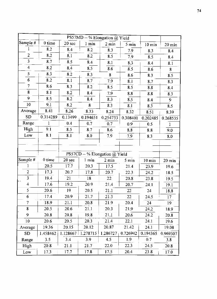
74
PS57MD - % Elongation (a) Yield
Sample # Otime 20 sec 1 min 2 min 5 min 10 min 20 min
1 8.2 8.4 8.2 8.3 7.9 8.3 8.4
2 8.2 8.1 8.2 8.5 7.9 8.5 8.4
3 8.7 8.5 8.4 8.1 8.3 8.4 8.1
4 8.2 8.4 8.5 8.6 8.5 8.6 8
5 8.3 8.2 8.3 8 8.6 8.3 8.5
6 8.2 8.1 8.7 7.9 8.1 8.7 8.3
7 8.6 8.3 8.2 8.5 8.5 8.8 8.4
8 8.1 8.2 8.4 7.9 8.8 8.8 8.3
9 8.5 8.2 8.4 8.3 8.5 8.4 9
10 9.1 8.2 8 8.3 8.1 8.3 8.5
Average 8.41 8.26 8.33 8.24 8.32 8.51 8.39
SD 0.314289 0.13499 0.194651 0.254733 0.308401 0.202485 0.268535
Range 1 0.4 0.7 0.7 0.9 0.5 1
High 9.1 8.5 8.7 8.6 8.8 8.8 9.0
Low 8.1 8.1 8.0 7.9 7.9 8.3 8.0
PS57CD - % Elongation @ Yield
Sample # Otime 20 sec 1 min 2 min 5 min 10 min 20 min
1 20.5 17.7 20.3 17.5 21.4 23.9 19.6
2 17.3 20.7 17.8 20.7 22.3 24.2 18.5
3 19.4 21 18 22 20.8 23.8 19.5
4 17.6 19.2 20.9 21.4 20.7 24.1 19.1
5 20.6 19 20.5 21.1 22 24 18.8
6 17.4 20.9 21.7 21.3 22 24.5 17
7 18.9 21.1 20.8 21.9 20.4 24 19
8 20.5 20.6 21.1 20.3 21.9 24.2 18.9
9 20.8 20.8 19.8 21.1 20.6 24.2 20.8
10 20.6 20.5 20.3 21.4 22.1 24.1 19.6
Average 19.36 20.15 20.12 20.87 21.42 24.1 19.08
SD 1.458462 1.128667 1.278715 1.286727 0.726942 0.194365 0.969307
Range 3.5 3.4 3.9 4.5 1.9 0.7 3.8
High 20.8 21.1 21.7 22.0 22.3 24.5 20.8
Low 17.3 17.7 17.8 17.5 20.4 23.8 17.0

75
PP50MD - % Elongation (o> Yield
Sample # 0 time 20 sec 1 min 2 min 5 min 10 min 20 min
1 18.5 18.4 17.2 18.3 18.2 18.9 19.3
2 19 18.9 17 18.5 18.5 18.5 18.7
3 19.5 18.3 16.6 18.5 18.6 19.2 18.8
4 18.6 18.3 18.4 18.3 18.6 19.3 19.6
5 18.6 19.3 18.8 18.7 19 18.9 18.7
6 18.1 17.8 18.1 18.5 18.1 19 19.2
7 18.4 18 18.3 17.3 19.1 19.3 19.2
8 19.5 18.8 18.2 17.8 19 19.3 19.2
9 19.3 18.3 18.8 18.7 19.4 19 19.1
10 19.3 18.4 18.3 18.4 19 18.4 19.3
Average 18.88 18.45 17.97 18.3 18.75 18.98 19.11
SD 0.502881 0.440328 0.764562 0.434613 0.417 0.32249 0.292309
Range 1.4 1.5 2.2 1.4 1.3 0.9 0.9
High 19.5 19.3 18.8 18.7 19.4 19.3 19.6
Low 18.1 17.8 16.6 17.3 18.1 18.4 18.7
PP50CD - % Elongation @ Yield
Sample # 0 time 20 sec 1 min 2 min 5 min 10 min 20 min
1 18.2 17.7 17.7 18.1 17.8 19.1 18.6
2 18.4 17.4 17.3 18.8 17.4 18.5 19.2
3 17.9 17.7 17.9 18.4 18.2 17.9 19.2
4 18.3 17.8 17.5 18.3 18 18 18.5
5 17.9 17.7 18 18.9 18.2 18.7 18.8
6 19.4 17.7 17.5 17.9 17.8 18.3 19.3
7 17.4 18.2 18.4 18.7 17.6 19.1 19.6
8 17.7 17.8 18.1 18 18.1 19.1 19.1
9 17.9 18.4 18.3 18.2 17.8 18.9 19
10 17.3 18.8 17.4 17.8 18.1 18.6 18.2
Average 18.04 17.92 17.81 18.31 17.9 18.62 18.95
SD 0.596657 0.418463 0.387155 0.384274 0.266667 0.446716 0.422295
Range 2.1 1.4 1.1 1.1 0.8 1.2 1.4
High 19.4 18.8 18.4 18.9 18.2 19.1 19.6
Low 17.3 17.4 17.3 17.8 17.4 17.9 18.2

76
PP55MD - % Elongation @ Yield
Sample # Otime 20 sec 1 min 2 min 5 min 10 min 20 min
1 18.4 18.2 18.3 17.6 19 18.6 17.9
2 18.2 18.3 18.1 17.9 19.5 19.4 19.1
3 18.8 17.5 18.1 16.5 19.3 18.9 18.9
4 19 17.7 18.3 16.7 17.7 19.2 19.6
5 17.9 17.2 18.2 18 17.7 18.9 19
6 18.2 17.9 18.2 18.1 18.2 18.7 18.8
7 18.6 17.3 18.8 17.8 18.1 19.3 19.4
8 18.6 18 18.1 17.9 18.8 18.2 18.9
9 19 18.2 18.2 17.7 18.3 18.5 17.9
10 18.5 17.4 18.6 17.9 19.3 19.5 18.3
Average 18.52 17.77 18.29 17.61 18.59 18.92 18.78
SD 0.358391 0.405654 0.233095 0.55267 0.675689 0.426354 0.578888
Range 1.1 1.1 0.7 1.6 1.8 1.3 1.7
High 19.0 18.3 18.8 18.1 19.5 19.5 19.6
Low 17.9 17.2 18.1 16.5 17.7 18.2 17.9
PP55CD - % Elongation @ Yield
Sample # 0 time 20 sec 1 min 2 min 5 min 10 min 20 min
1 16.7 16.6 17.2 17.5 17.5 17.6 18.2
2 16.5 17.3 17.9 17.7 16.5 18.1 18.6
3 16.5 17.7 17.7 16.7 16.8 18.2 18.3
4 16.7 16.8 17.6 18.2 17 18 18.3
5 16.1 16.7 17.7 16.8 17.2 18.3 18.2
6 16.4 17.1 17.9 18.2 17.1 17.8 18.2
7 16.4 16.7 18.1 17.7 17.5 17.8 18.2
8 16.8 17.7 17.9 17.5 18.6 18.2 18.1
9 16.6 16.9 17.7 17.3 18.1 17.8 18.1
10 17.4 17.5 18.1 17.1 18.2 18 18.2
Average 16.61 17.1 17.78 17.47 17.45 17.98 18.24
SD 0.341402 0.424264 0.265832 0.51435 0.668747 0.225093 0.142984
Range 1.3 1.1 0.9 1.5 2.1 0.7 0.5
High 17.4 17.7 18.1 18.2 18.6 18.3 18.6
Low 16.1 16.6 17.2 16.7 16.5 17.6 18.1

77
PS52MD - Modulus ofElasticitySample # Otime 20 sec 1 min 2 min 5 min 10 min 20 min
1 77273 77826 74726 82901 83902 84212 84338
2 78638 78638 75851 81734 77400 77206 83283
3 81544 80044 76471 79877 79997 78446 76780
4 76276 79066 76471 75852 75542 72137 76471
5 76896 77826 78329 78948 79377 76471 76276
6 78638 80360 81425 75852 80186 75233 78446
7 83097 80496 70075 76276 80902 78019 75543
8 80805 79397 78948 83097 76830 76471 78329
9 83718 77546 76471 82972 77206 77400 79220
10 85140 77826 72756 84265 83283 80806 75232
Average 80202.5 78902.5 76152.3 80177.4 79462.5 77640.1 78391.8
SD 3111.021 1136.488 3184.225 3285.052 2765.664 3215.652 3141.795
Range 8864 2950 11350 8413 8360 12075 9106
High 85140 80496 81425 84265 83902 84212 84338
Low 76276 77546 70075 75852 75542 72137 75232
PS52CD - Modulus ofElasticitySample # 0 time 20 sec 1 min 2 min 5 min 10 min 20 min
1 54210 53870 55191 54180 56432 54799 56038
2 56656 58824 52013 55191 54881 55728 54798
3 55728 56432 52942 53560 56656 56657 55894
4 58419 56348 53951 54881 54489 53251 52941
5 54489 55419 57538 54489 54180 53319 55811
6 58205 55109 56122 55418 56122 57585 55108
7 58514 55191 58514 58205 58824 57895 53728
8 58292 59481 57585 57052 55727 56432 55418
9 52941 56742 55108 57672 52632 55091 54799
10 55191 53560 54799 55191 53561 54180 55728
Average 56264.5 56097.6 55376.3 55583.9 55350.4 55493.7 55026.3
SD 2043.715 1918.674 2099.238 1544.952 1782.675 1651.866 1010.089
Range 5573 5921 6501 4645 6192 4644 3097
High 58514 59481 58514 58205 58824 57895 56038
Low 52941 53560 52013 53560 52632 53251 52941

78
PS57MD - Modulus ofElasticitySample # 0 time 20 sec 1 min 2 min 5 min 10 min 20 min
1 82472 77954 79648 77575 82191 82880 76542
2 83728 83603 80496 78236 81359 73262 79931
3 77515 74394 78518 85708 80617 78237 81343
4 80213 76374 80900 79932 79084 73435 81626
5 80213 79083 76542 83885 75694 77222 76091
6 80051 77034 78637 86557 75420 71565 77389
7 77788 76824 82473 80617 75242 73357 74847
8 85426 78801 77222 80213 72414 73152 77671
9 80617 81626 76374 76374 78637 73152 76114
10 72697 82473 80634 75413 75573 75730 78236
Average 80072 78816.6 79144.4 80451 77623.1 75199.2 77979
SD 3563.307 2937.51 2034.538 3833.278 3206.429 3406.606 2305.876
Range 12729 9209 6099 11144 9777 11315 6779
High 85426 83603 82473 86557 82191 82880 81626
Low 72697 74394 76374 75413 72414 71565 74847
PS57CD ~ Modulus ofElasticitySample # 0 time 20 sec 1 min 2 min 5 min 10 min 20 min
1 50274 50274 49965 49145 48653 50275 50388
2 50067 50840 49145 47804 48862 49501 49992
3 50840 50850 49095 48223 49710 49992 49710
4 51482 50558 50274 46107 50275 48653 49709
5 48936 49715 47884 49427 49501 48579 48015
6 50839 48862 51199 50382 50350 49427 50557
7 51687 46673 48298 46480 51122 49338 49710
8 50817 50350 50275 47732 48297 46320 48862
9 50916 47521 52252 49427 49144 48653 48580
10 51122 48580 50237 48862 49784 48580 50274
Average 50698 49422.3 49862.4 48358.9 49569.8 48931.8 49579.7
SD 785.7667 1460.849 1310.308 1356.727 864.6415 1099.879 834.9293
Range 2751 4177 4368 4275 2825 3955 2542
High 51687 50850 52252 50382 51122 50275 50557
Low 48936 46673 47884 46107 48297 46320 48015

79
PP50MD - Modulus ofElasticitySample # Otime 20 sec 1 min 2 min 5 min 10 min 20 min
1 87916 91784 85671 91716 86189 75493 86756
2 86240 91986 94420 83482 84513 77298 88250
3 81681 92243 82224 83482 84257 81133 88120
4 78377 90621 89666 78506 83998 79150 83533
5 81038 84694 85256 83791 82583 78846 80779
6 87091 92815 82966 82324 89463 83870 85983
7 87090 94877 88174 94749 87220 72963 84384
8 77300 89979 86369 82707 88948 82581 85544
9 79618 88948 84256 85390 87220 82839 86203
10 78377 90440 86446 87787 81342 76443 85338
Average 82472.8 90838.7 86544.8 85393.4 85573.3 79061.6 85489
SD 4184.774 2721.787 3552.712 4797.924 2677.166 3559.273 2215.132
Range 10616 10183 12196 16243 8121 10907 7471
High 87916 94877 94420 94749 89463 83870 88250,
Low 77300 84694 82224 78506 81342 72963 80779
PP50CD - Modulus ofElasticitySample # 0 time 20 sec 1 min 2 min 5 min 10 min 20 min
1 86447 88766 90182 90183 83999 84022 81213
2 82583 84128 84951 81808 86189 78377 79747
3 87605 85029 81604 78588 81937 81060 77944
4 85287 85415 83662 83998 80649 78974 77217
5 85029 85545 84514 83999 82373 79490 74595
6 71374 79408 83026 80817 87605 78974 78459
7 83612 88819 81084 85030 75497 78020 72090
8 86498 85803 82195 83096 78119 79490 80711
9 83999 79279 85030 78331 82711 79360 78893
10 85080 86561 83998 82502 78248 80262 81342
Average 83751.4 84875.3 84024.6 82835.2 81732.7 79802.9 78221.1
SD 4595.429 3281.672 2560.499 3418.051 3743.85 1718.201 2973.055
Range 16231 9540 9098 11852 12108 6002 9252
High 87605 88819 90182 90183 87605 84022 81342
Low 71374 79279 81084 78331 75497 78020 72090

80
PP55MD - Modulus ofElasticitySample # Otime 20 sec 1 min 2 min 5 min 10 min 20 min
1 90471 93461 87723 93228 85967 85315 900662 89597 92102 91291 93110 85849 85783 856163 87020 95184 86669 83972 86252 86318 855494 84561 90652 87841 95804 90588 83859 75969
5 87934 94750 90769 91119 92698 88244 86955
6 85783 91588 86955 87255 88427 88289 83205
7 85966 94221 79808 86201 88661 83624 84377
8 86435 89479 88659 89862 85549 88192 87254
9 87541 88660 89246 88075 88191 86252 85592
10 89416 91003 86369 80393 85616 81372 86366
Average 87472.4 92110 87533 88901.9 87779.8 85724.8 85094.9
SD 1896.819 2239.767 3180.471 4682.067 2413.988 2276.722 3689.975
Range 5910 6524 11483 15411 7149 6917 14097
High 90471 95184 91291 95804 92698 88289 90066
Low 84561 88660 79808 80393 85549 81372 75969
PP55CD - Moduliis ofElastic;ity
Sample # 0 time 20 sec 1 min 2 min 5 min 10 min 20 min
1 93110 82571 85966 88309 89246 83975 85498
2 89245 87658 83858 82571 92932 81867 81447
3 86955 81516 89065 91822 83155 79642 75426
4 86709 90299 86135 82920 88191 80930 82799
5 82736 90651 87021 89246 87372 83155 84494
6 88713 88778 78238 87020 88074 83674 83975
7 86669 91588 81399 89534 88948 83624 83791
8 85029 88191 84677 90095 78166 82385 83273
9 81985 90471 85967 86955 83322 84678 83506
10 82335 85901 80275 87541 78704 82335 82922
Average 86348.6 87762.4 84260.1 87601.3 85811 82626.5 82713.1
SD 3499.818 3454.612 3345.255 2961.827 4804.811 1524.036 2776.48
Range 11125 10072 10827 9251 14766 5036 10072
High 93110 91588 89065 91822 92932 84678 85498
Low 81985 81516 78238 82571 78166 79642 75426
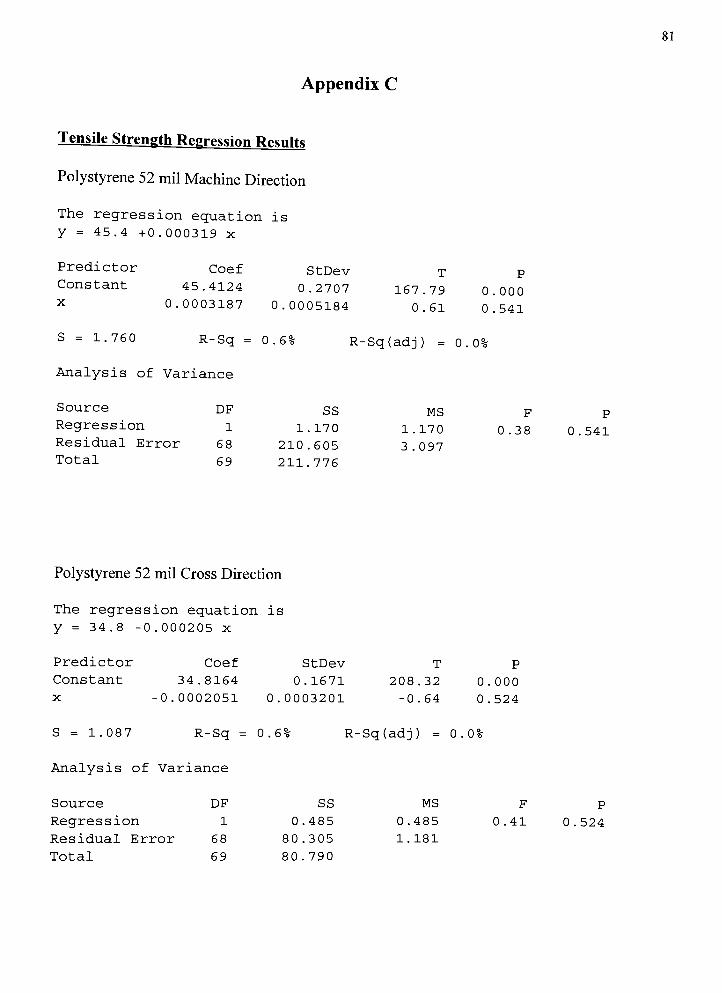
81
Appendix C
Tensile Strength Regression Results
Polystyrene 52 mil Machine Direction
The regression equation is
y = 45.4 +0.000319 x
Predictor Coef StDev T P
Constant 45.4124 0 .2707 167.79 0.000X 0.0003187 0 . 0005184 0.61 0.541
S = 1.760 R-Sq = 0.6%
Analysis of Variance
R-Sq(adj) = 0.0%
Source DF SS MS F P
Regression 1 1..170 1.170 0.38 0.541
Residual Error 68 210..605 3 .097
Total 69 211.,776
Polystyrene 52 mil Cross Direction
The regression equation is
y = 34.8 -0.000205 x
Predictor Coef StDev T P
Constant 34.8164 0.1671 208 .32 0.000
X -0.0002051 0. 0003201 -0.64 0.524
S = 1.087 R-Sq
Analysis of Variance
=0.6*
R-Sq(adj) =0.0%
Source DF SS MS F P
Regression 1 0.485 0.485 0 .41 0.524
Residual Error 68 80.305 1.181
Total 69 80.790

82
Polystyrene 57 mil Machine Direction
The regression equation is
y = 51.0 -0.000182 x
Predictor coef StDev
Constant 51.0182 0.2422
x-0.0001823 0.0004639
T
210.63
-0.39
S = 1.575 R-Sq = 0.2^
Analysis of Variance
P
0.000
0.696
R-Sq(adj) =0.0%
Source DF SS MS F P
Regression 1 0 .383 0.383 0.15 0.696Residual Error 68 168..671 2 .480
Total 69 169..054
Polystyrene 57 mil Cross Direction
The regression equation is
y = 36.7 -0.000314 x
Predictor Coef StDev T P
Constant 36.7346 0. 0587 625.76 0.000
X -0.0003140 0. 0001124 -2.79 0.007
S = 0.3817 R-Sq = 10.3%
Analysis of Variance
R-Sq(adj) =9.0%
Source DF
Regression 1
Residual Error 68
Total 69
SS MS F P
1..1365 1.1365 7.80 0.007
9..9079 0.1457
11,, 0445
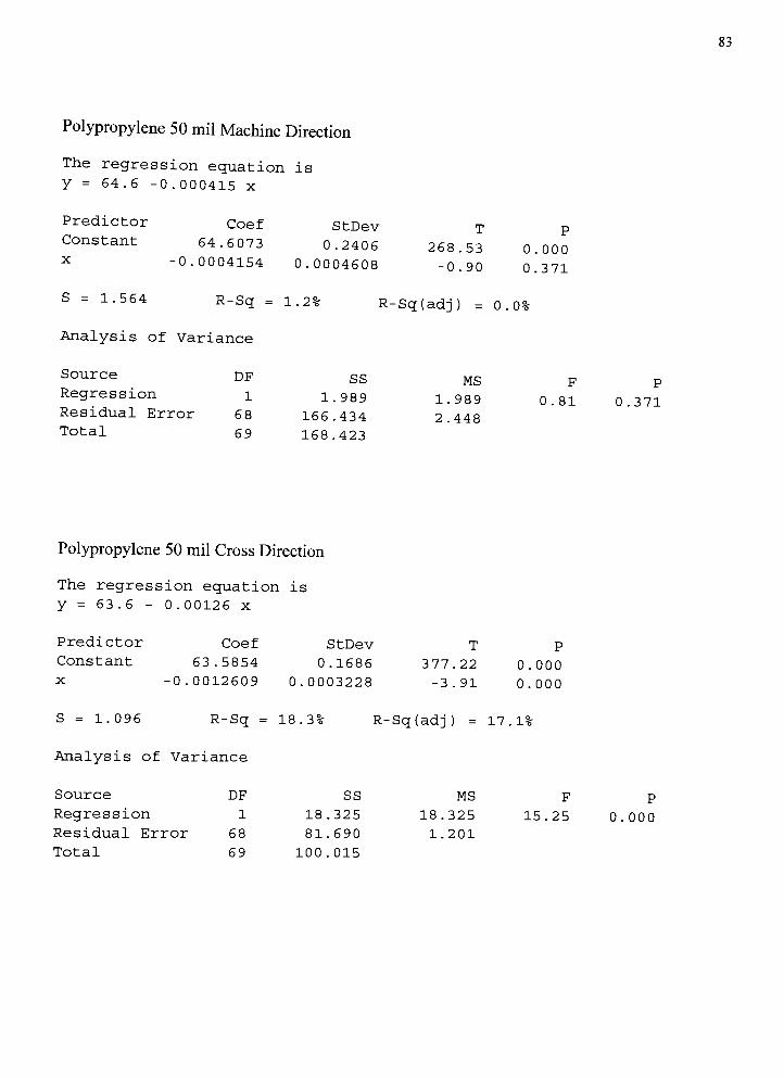
83
Polypropylene 50 mil Machine Direction
The regression equation is
y = 64.6 -0.000415 x
Predictor Coef StDev T pConstant 64.6073 0.2406 268.53 0.000X
-0.0004154 0.0004608 -0.90 0.371
S = 1.564 R-Sq = 1.2% R-Sq(adj) = 0.0%
Analysis of Variance
Source DF SS MS F P
Regression
Residual Error
1
68
1.989
166.434
1.989
2 .448
0.81 0.371
Total 69 168.423
Polypropylene 50 mil Cross Direction
The regression equation is
y = 63 .6 - 0 .00126 x
Predictor Coef StDev T P
Constant 63.5854 0.1686 377.22 0.000
X -0. 0012609 0.0003228 -3.91 0.000
S = 1.096 R-Sq = 18.3% R-Sq(adj) = 17.1%
Analysis of Variance
Source DF SS MS F P
Regression 1 18 .325 18.325 15.25 0.000
Residual Error 68 81..690 1.201
Total 69 100,,015

84
Polypropylene 55 mil Machine Direction
The regression equation is
y = 73 .0 -0.000195 x
Predictor
Constant
X
Coef
72.9899
-0 .0001949
StDev
0.1717
0.0003288
T
425.10
-0.59
P
0.000
0.555
S = 1.H6 R-Sq = 0.5% R--Sq(adj) = 0,.0%
Analysis of Variance
Source DF SS MS F P
Regression 1 0.438 0.438 0.35 0.555Residual Error 68 84.759 1.246
Total 69 85.197
Polypropylene 55 mil Cross Direction
The regression equation is
y = 72.0 -0.000668 x
Predictor Coef StDev T P
Constant 71.9752 0.1428 503.97 0.000
X -0 .0006684 0 . 0002735 -2.44 0.017
S = 0.9286 R-Sq = 8.1%
Analysis of Variance
R-Sq(adj) =6.7%
Source DF SS MS F P
Regression 1 5 .1492 5.1492 5.97 0.017
Residual Error 68 58,.6406 0.8624
Total 69 63 ..7897
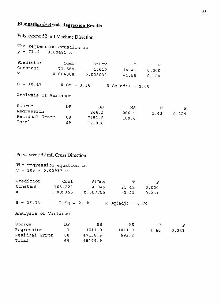
85
Elongation (a). Break Regression Results
Polystyrene 52 mil Machine Direction
The regression equation is
y = 71.6 -
0.00481 x
Predictor Coef StDev T p
Constant 71.564 1.610 44.45 0.000X
-0.004808 0.003083 -1.56 0.124
S = 10.47 R-Sq = 3.5%
Analysis of Variance
R-Sq(adj) =2.0=
Source DF SS MS F P
Regression 1 266.5 266.5 2.43 0.124Residual Error 68 7451.5 109.6
Total 69 7718 .0
Polystyrene 52 mil Cross Direction
The regression equation is
y = 103 - 0.00937 x
Predictor Coef StDev
Constant 103.221 4.049
x -0.009365 0.007755
T
25.49
-1.21
S = 26.33 R-Sq = 2.11
Analysis of Variance
P
0.000
0.231
R-Sq(adj) =0.7%
Source DF SS MS F P
Regression 1 1011.0 1011.0 1.46 0.231
Residual Error 68 47138.9 693.2
Total 69 48149.9

86
Polystyrene 57 mil Machine Direction
The regression equation is
y = 82.8 -
0.00666 x
Predictor
Constant
X
Coef
82 .758
-0.006664
StDev
3.356
0.006428
T
24.66
-1.04
P
0.000
0.304
S = 21.82 R-Sq = 1.6% R--Sq(adj) = 0,.1%
Analysis of Variance
Source DF SS MS F P
Regression 1 511.9 511.9 1.07 0.304
Residual Error 68 32385.7 476.3
Total 69 32897.6
Polystyrene 57 mil Cross Direction
The regression equation is
y = 81. 9 - 0 .00760 x
Predictor Coef StDev
Constant 81.935 4.810
x -0.007599 0.009212
T P
17.03 0.000
-0.82 0.412
S = 31.28 R-Sq = 1.01
Analysis of Variance
R-Sq(adj) =0.01
Source DF SS MS F P
Regression 1 665.7 665.7 0.68 0.412
Residual Error 68 66521.3 978.3
Total 69 67186.9

87
Polypropylene 50 mil Machine Direction
The regression equation is
y = 408 + 0.163 x
Predictor Coef StDev T p
Constant 407.71 37.86 10.77 0.000X 0.16259 0.07251 2 .24 0.028
S = 246.2 R-Sq = 6.9% R--Sq(adj) = 5,.5%
Analysis of Variance
Source DF SS MS F P
Regression 1 304711 304711 5.03 0.028Residual Error 68 4121040 60604
Total 69 4425750
Polypropylene 50 mil Cross Direction
The regression equation is
y = 562 - 0 .044 x
Predictor Coef StDev T P
Constant 561.74 55.04 10.21 0.000
X -0.0438 0.1054 -0.42 0.679
S = 357.9 R-Sq = 0.3% R-Sq(adj) = 0.01
Analysis of Variance
Source DF SS MS F P
Regression 1 22070 22070 0.17 0.679
Residual Error 68 8710564 128097
Total 69 8732635

88
Polypropylene 55 mil Machine Direction
The regression equation is
y = 228 -
0.0530 x
Predictor Coef StDev T p
Constant 228.49 14.92 15.32 0.000X
-0.05299 0.02857 -1.85 0.068
S = 97.00 R-Sq = 4.8%
Analysis of Variance
R-Sq(adj) = 3.4%
Source DF SS MS F P
Regression 1 32365 32365 3 .44 0.068Residual Error 68 639870 9410
Total 69 672235
Polypropylene 55 mil Cross Direction
The regression equation is
y = 43.7 + 0.172 x
Predictor Coef StDev T P
Constant 43.70 17.98 2.43 0.018
X 0. 17164 0.03444 4.98 0.000
S = 116.9 R-Sq = 26.8%
Analysis of Variance
R-Sq(adj) = 25.7%
Source DF SS MS F P
Regression 1 339583 339583 24.84 0.000
Residual Error 68 929775 13673
Total 69 1269358

89
Elongation @ Yield Regression Results
Polystyrene 52 mil Machine Direction
The regression equation is
y = 8.23 +0.000222 x
Predictor
Constant
x
Coef StDev
8.23133 0.04286
0.00022204 0.00008208
T
192.07
2 .71
P
0.000
0.009
S = 0.2787 R-Sq = 9.7%
Analysis of Variance
R-Sq(adj) = 8.4%
Source DF SS MS F pRegression 1 0 .56830 0.56830 7.32 0.009Residual Error 68 5,.28042 0.07765
Total 69 5..84871
Polystyrene 52 mil Cross Direction
The regression equation is
y = 12.0 +0.000059 x
Predictor Coef StDev
Constant 11.9721 0.3898
x 0.0000587 0.0007465
T
30.71
0. 08
S = 2.535 R-Sq =0.0%
Analysis of Variance
P
0.000
0.938
R-Sq(adj) =0.0%
Source DF SS MS F P
Regression 1 0 .040 0.040 0.01 0.938
Residual Error 68 436..815 6.424
Total 69 436.,855
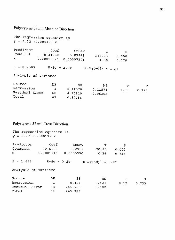
90
Polystyrene 57 mil Machine Direction
The regression equation is
y = 8.32 +0.000100 x
Predictor Coef
Constant 8.31850 0.03849 216.13x 0.00010021 0.00007371
_.36
S = 0.2503 R-Sq = 2.6% R-Sq(adj
StDev t p
0.000
0.178
1.2%
Analysis of Variance
Source DF SS MS F P
Regression 1 0 .11576 0.11576 1.85 0.178Residual Error 68 4 ,.25910 0.06263
Total 69 4,.37486
Polystyrene 57 mil Cross Direction
The regression equation is
y = 20.7 +0.000192 x
Predictor Coef StDev T p
Constant 20.6656 0.2919 70.80 0.000
x 0.0001916 0.0005590 0.34 0.733
S = 1.898 R-Sq = 0.2% R-Sq(adj) = 0.0%
Analysis of Variance
Source DF SS MS F P
Regression 1 0 .423 0.423 0.12 0.733
Residual Error 68 244 .960 3.602
Total 69 245.383

91
Polypropylene 50 mil Machine Direction
The regression equation is
y = 18.4 +0.000633 x
Predictor
Constant
X
Coef
18.4264
0. 0006327
StDev
0. 0828
0. 0001585
T
222.59
3.99
P
0.000
0.000
S = 0.5383 R-Sq = 19.0% R--Sq(adj) = 17 .8%
Analysis of Variance
Source DF SS MS F P
Regression 1 4 .6148 4.6148 15.93 0.000Residual Error 68 19,.7029 0.2897
Total 69 24,.3177
Polypropylene 50 mil Cross Direction
The regression equation is
y = 17.9 +0 .000865 x
Predictor Coef StDev T P
Constant 17.9373 0.0693 258.76 0.000
X 0. 0008649 0.0001328 6.51 0. 000
S = 0.4507 R-Sq = 38.4% R-Sq(adj) = 37.51
Analysis of Variance
Source DF SS MS F P
Regression 1 8 .6219 8.6219 42.44 0.000
Residual Error
Total
68
69
13
22,
.8159
.4379
0.2032
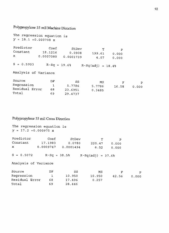
92
Polypropylene 55 mil Machine Direction
The regression equation is
y = 18.1 +0.000708 x
Predictor
Constant
x
Coef StDev
18.1216 0.0908
0.0007080 0.0001739
S = 0.5903 R-Sq = 19.6%
Analysis of Variance
T P
199.61 0.000
4.07 0.000
R-Sq(adj) = 18.4%
Source DF SS MS
Regression 1 5 .7786 5.7786
Residual Error 68 23 ..6951 0.3485
Total 69 29,.4737
16.5}
P
0.000
Polypropylene 55 mil Cross Direction
The regression equation is
y = 17.2 +0 . 000975 x
Predictor Coef StDev T P
Constant 17.1983 0.0780 220.47 0.000
X 0. 0009747 0 . 0001494 6.52 0. 000
S = 0.5072 R-Sq = 38.5%
Analysis of Variance
R-Sq(adj) = 37.61
Source DF SS MS F P
Regression 1 10 .950 10.950 42.56 0.000
Residual Error 68 17..496 0.257
Total 69 28,.446
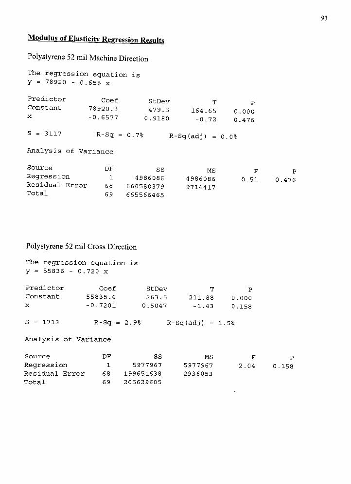
93
Modulus ofElasticity Regression Results
Polystyrene 52 mil Machine Direction
The regression equation is
y = 78920 -
0.658 x
Predictor Coef StDev T p
Constant 78920.3 479.3 164.65 0.000X
-0.6577 0.9180 -0.72 0.476
S = 3117 R-Sq = 0.7%
Analysis of Variance
R-Sq(adj) =0.0%
Source DF SS MS F P
Regression 1 4986086 4986086 0.51 0.476Residual Error 68 660580379 9714417
Total 69 665566465
Polystyrene 52 mil Cross Direction
The regression equation is
y = 55836 - 0 .720 x
Predictor Coef StDev T P
Constant 55835.6 263.5 211.88 0.000
X -0.7201 0.5047 -1.43 0.158
S = 1713 R-Sq = 2.9%
Analysis of Variance
R-Sq(adj) =1.5%
Source DF SS MS F P
Regression 1 5977967 5977967 2.04 0 .158
Residual Error 68 199651638 2936053
Total 69 205629605
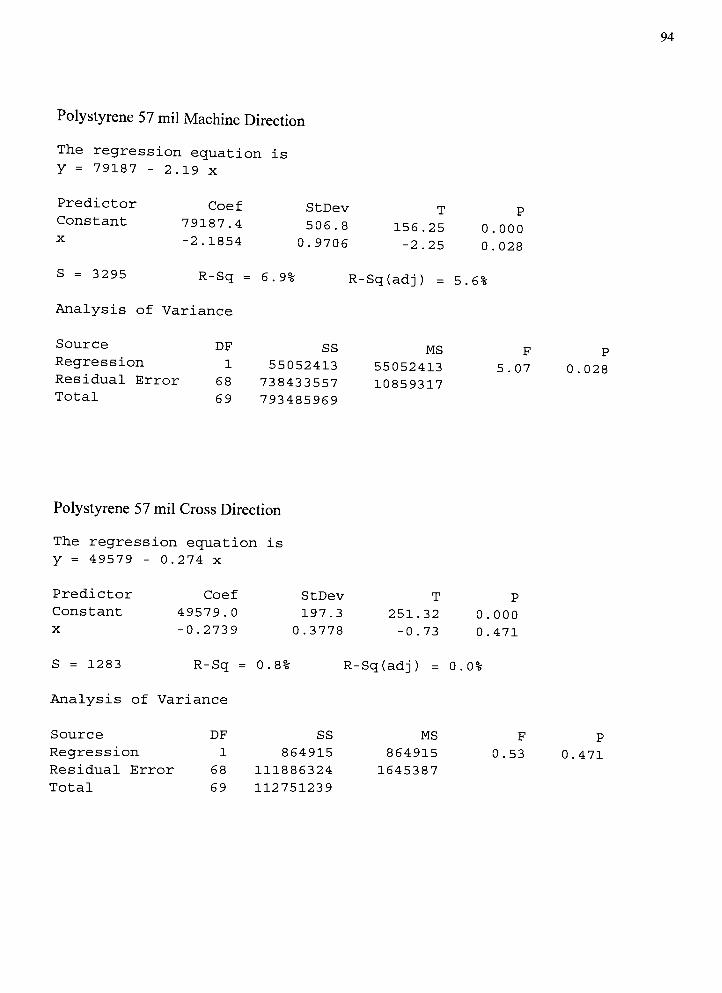
94
Polystyrene 57 mil Machine Direction
The regression equation is
y = 79187 - 2.19 x
Predictor
Constant
x
Coef
79187.4
-2.1854
StDev
506.8
0.9706
S = 3295 R-Sq = 6.9%
Analysis of Variance
T p
156.25 0.000
-2.25 0.028
R-Sq(adj) = 5.6%
Source DF SS MS F P
Regression 1 55052413 55052413 5.07 0.028Residual Error 68 738433557 10859317
Total 69 793485969
Polystyrene 57 mil Cross Direction
The regression equation is
y = 49579 - 0.274 x
Predictor Coef StDev T P
Constant 49579.0 197.3 251.32 0.000
X -0.2739 0.3778 -0.73 0.471
S = 1283 R-Sq = 0.8%
Analysis of Variance
R-Sq(adj) =0.0%
Source DF SS MS F P
Regression 1 864915 864915 0.53 0.471
Residual Error 68 111886324 1645387
Total 69 112751239

95
Polypropylene 50 mil Machine Direction
The regression equation is
y = 85815 - 2.32 x
Predictor Coef StDev T P
Constant 85814.5 720.9 119.04 0.000X
-2.317 1.381 -1.68 0.098
S = 4688 R-Sq = 4.01
Analysis of Variance
R-Sq(adj) =2.61
Source DF SS MS F P
Regression 1 61861487 61861487 2.82 0.098
Residual Error 68 1494189016 21973368
Total 69 1556050502
Polypropylene 50 mil Cross Direction
The regression equation is
y = 83906 - 5.26 x
Predictor Coef StDev T P
Constant 83905.7 498.8 168.20 0.000
X -5.2594 0.9554 -5.50 0.000
S = 3244 R-Sq = 30.81
Analysis of Variance
R-Sq(adj) = 29.81
Source DF SS MS F P
Regression 1 318844433 318844433 30.30 0.000
Residual Error 68 715456936 10521426
Total 69 1034301369
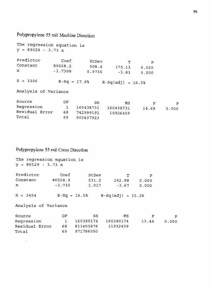
96
Polypropylene 55 mil Machine Direction
The regression equation is
y = 89028 - 3.73 x
Predictor Coef StDev t p
Constant 89028 .2 508.4 175.13 0.000X
-3.7308 0.9736 -3.83 0.000
S = 3306 R-Sq = 17.8% R-Sq(adj) = 16 .5%
Analysis of Variance
Source DF SS MS F P
Regression 1 160438731 160438731 14.68 0.000
Residual Error 68 742999191 10926459
Total 69 903437923
Polypropylene 55 mil Cross Direction
The regression equation is
y = 86529 - 3 .73 x
Predictor Coef StDev T P
Constant 86528.9 531.2 162.88 0.000
X -3.730 1.017 -3.67 0.000
S = 3454 R-Sq = 16.5%
Analysis of Variance
R-Sq(adj) = 15.3%
Source DF SS MS F P
Regression 1 160380174 160380174 13 .44 0.000
Residual Error 68 811405876 11932439
Total 69 971786050

97
Appendix D
SEM Photographs
US'*'
:,
Polystyrene 52 mil Sample - 10,000x magnification - PS side @ zero time (control)
"?
. .".,;. '.
/.'
Polystyrene 52 mil Sample- 10,000x magnification
- PS side @ 20 minutes (variable)

98
-
v:?-::
>:"-.
0
'..
-
..-
-
'
:;;SiA "-''
.--.-,
:'a^:A:'4a .
-::..i-'-'-b'-;.'vV.-:
A^'^At^^A^A:A0AEAAA:\.-: -^ J . ;if : ; ;^;
Polypropylene 50 mil Sample - 10,000x magnification - PP side @ zero time (control)
Polypropylene 50 mil Sample - 10,000x magnification - PP side @ 20 minutes (variable)

99
Appendix E
Tensile Strength ANQVA Results
Polystyrene 52 mil Machine Direction
Anova: Single Factor
SUMMARY
Groups Count Sum Average VarianceColumn 1
Column 2
Column 3
Column 4
Column 5
Column 6
Column 7
10
10
10
10
10
10
10
460.99
451.43
438.16
463.11
460.44
454.9
457.17
46.099
45.143
43.816
46.311
46.044
45.49
45.717
2.990476667
0.328978889
2.651893333
3.032165556
2.866471111
3.743911111
3.115756667
ANOVA
Source of Variation SS df MS F P-value F crit
Between Groups
Within Groups
Total
43.20894857
168.56688
211.7758286
6
63
69
7.201491429
2.675664762
2.691477472 0.02170913 2.246409281
Polystyrene 52 mil Cross Direction
Anova: Single Factor
SUMMARY
Groups Count Sum Average Variance
Column 1 10 350.21 35.021 1.157276667
Column 2 10 350.24 35.024 1.364782222
Column 3 10 346.61 34.661 1 .252654444
Column 4 10 345.77 34.577 0.97209
Column 5 10 344.15 34.415 1.154494444
Column 6 10 350.36 35.036 1.131426667
Column 7 10 345.09 34.509 1.456721111
ANOVA
Source of Variation SS df MS F P-value F crit
Between Groups 4.38462 6 0.73077 0.602558785 0.72722343 2.246409281
Within Groups 76.40501 63 1.212777937
Total 80.78963 69
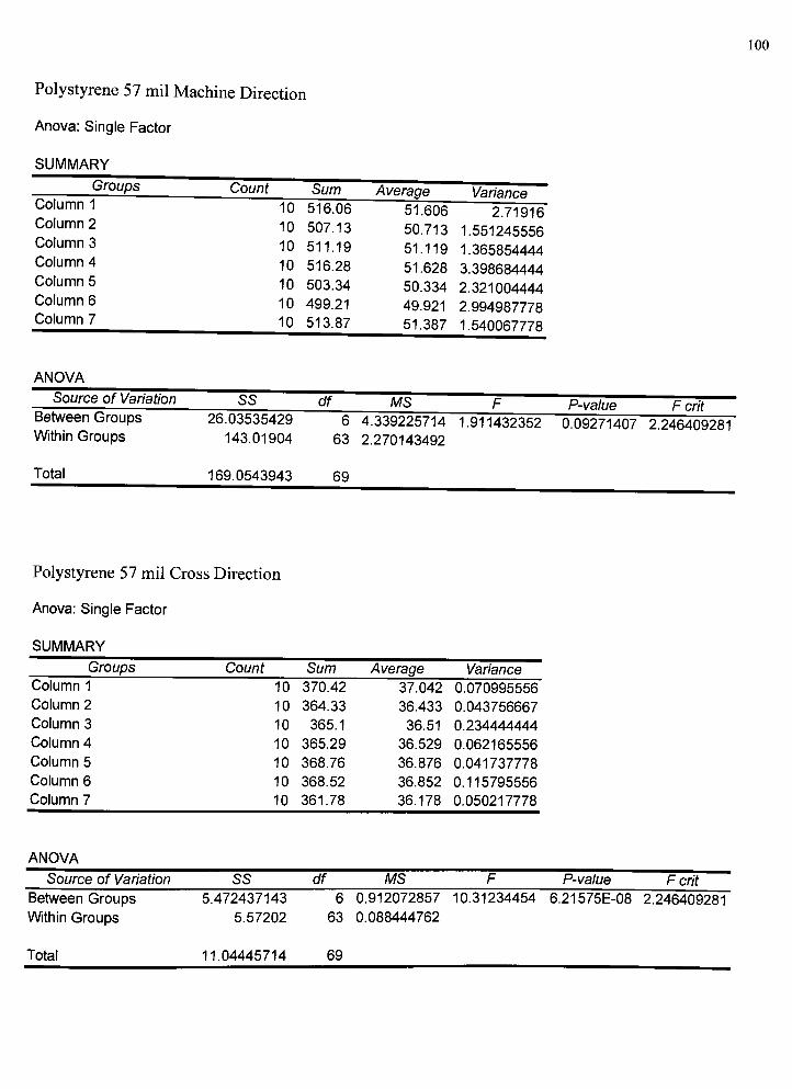
100
Polystyrene 57 mil Machine Direction
Anova: Single Factor
SUMMARY
Groups Count Sum Average VarianceColumn 1
Column 2
Column 3
Column 4
Column 5
Column 6
Column 7
10
10
10
10
10
10
10
516.06
507.13
511.19
516.28
503.34
499.21
513.87
51.606
50.713
51.119
51.628
50.334
49.921
51.387
2.71916
1.551245556
1.365854444
3.398684444
2.321004444
2.994987778
1.540067778
ANOVA
Source of Variation SS df MS F P-value F critBetween Groups
Within Groups
Total
26.03535429
143.01904
169.0543943
6
63
69
4.339225714
2.270143492
1.911432352 0.09271407 2.246409281
Polystyrene 57 mil Cross Direction
Anova: Single Factor
SUMMARY
Groups Count Sum Average Variance
Column 1
Column 2
Column 3
Column 4
Column 5
Column 6
Column 7
10 370.42 37.042 0.070995556
10 364.33 36.433 0.043756667
10 365.1 36.51 0.234444444
10 365.29 36.529 0.062165556
10 368.76 36.876 0.041737778
10 368.52 36.852 0.115795556
10 361.78 36.178 0.050217778
ANOVA
Source of Variation SS df MS P-value F crit
Between Groups
Within Groups
5.472437143
5.57202
6 0.912072857
63 0.088444762
10.31234454 6.21575E-08 2.246409281
Total 11.04445714 69
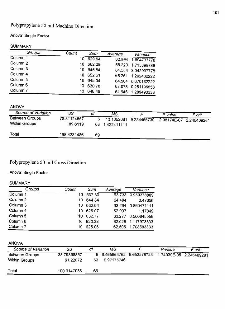
101
Polypropylene 50 mil Machine Direction
Anova: Single Factor
SUMMARY
Groups Count Sum Average VarianceColumn 1
Column 2
Column 3
Column 4
Column 5
Column 6
Column 7
10
10
10
10
10
10
10
629.94
662.29
645.84
652.61
645.04
630.78
646.46
62.994
66.229
64.584
65.261
64.504
63.078
64.646
1.694737778
1.715898889
3.042937778
1.292432222
0.670182222
0.251195556
1.289493333
ANOVA
Source of Variation SS df MS F P-value F crit
Between Groups
Within Groups
Total
78.81124857
89.6119
168.4231486
6
63
69
13.1352081
1.422411111
9.234466739 2.981 74E-07 2.246409281
Polypropylene 50 mil Cross Direction
Anova: Single Factor
SUMMARY
Groups Count Sum Average Variance
Column 1
Column 2
Column 3
Column 4
Column 5
Column 6
Column 7
10
10
10
10
10
10
10
637.33
644.84
632.64
629.07
632.77
620.28
625.05
63.733
64.484
63.264
62.907
63.277
62.028
62.505
0.959378889
0.47056
0.860471111
1.17849
0.506845556
1.117973333
1.708583333
ANOVA
Source of Variation SS df MS P-value F crit
Between Groups
Within Groups
38.79398857 6 6.465664762 6.653578723 1.74039E-05 2.246409281
61.22072 63 0.97175746
Total 100.0147086 69
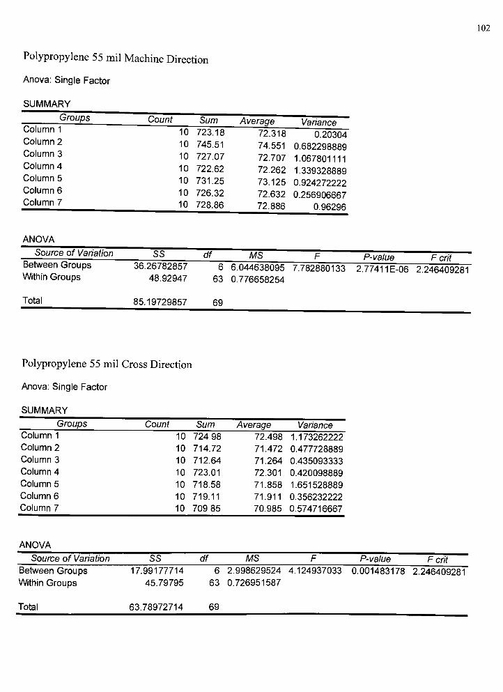
102
Polypropylene 55 mil Machine Direction
Anova: Single Factor
SUMMARY
Groups Count Sum Average VarianceColumn 1
Column 2
Column 3
Column 4
Column 5
Column 6
Column 7
10
10
10
10
10
10
10
723.18
745.51
727.07
722.62
731.25
726.32
728.86
72.318
74.551
72.707
72.262
73.125
72.632
72.886
0.20304
0.682298889
1.067801111
1.339328889
0.924272222
0.256906667
0.96296
ANOVA
Source of Variation SS df MS F P-value F crit
Between Groups
Within Groups
Total
36.26782857
48.92947
85.19729857
6
63
69
6.044638095
0.776658254
7.782880133 2.7741 1E-06 2.246409281
Polypropylene 55 mil Cross Direction
Anova: Single Factor
SUMMARY
Groups Count Sum Average Variance
Column 1
Column 2
Column 3
Column 4
Column 5
Column 6
Column 7
10
10
10
10
10
10
10
724.98
714.72
712.64
723.01
718.58
719.11
709.85
72.498
71.472
71.264
72.301
71.858
71.911
70.985
1.173262222
0.477728889
0.435093333
0.420098889
1.651528889
0.356232222
0.574716667
ANOVA
Source of Variation SS df MS P-value F crit
Between Groups
Wthin Groups
17.99177714 6 2.998629524 4.124937033
45.79795 63 0.726951587
0.001483178 2.246409281
Total 63.78972714 69

Elongation (a). Break ANOVA Results
103
Polystyrene 52 mil Machine Direction
Anova: Single Factor
SUMMARY
Groups Count Sum Average VarianceColumn 1
Column 2
Column 3
10
10
10
732.8
644.5
769.8
73.28
64.45
76.98
116.5306667
115.1183333
54.224Column 4 10 680 68 63.06Column 5
Column 6
10
10
736.2
683.4
73.62
68.34
129.1617778
95.24933333Column 7 10 652.2 65.22 136.444
ANOVA
Source of Variation SS df MS F P-value F crit
Between Groups
Within Groups
1329.879714
6388.093
6
63
221.646619
101.3983016
2.185900706 0.055951258 2.246409281
Total 7717.972714 69
Polystyrene 52 mil Cross Direction
Anova: Single Factor
SUMMARY
Groups Count Sum Average Variance
Column 1
Column 2
Column 3
Column 4
Column 5
Column 6
Column 7
10 1009.2 100.92 668.0062222
10 996.8 99.68 519.6128889
10 980 98 370.6644444
10 1022.6 102.26 822.2537778
10 1058 105.8 461.5888889
10 1092.8 109,28 1563.912889
10 850.7 85.07 552.1978889
ANOVA
Source of Variation SS df MS P-value F crit
Between Groups
Within Groups
3525.739714 6 587.6232857 0.829601933 0.551490649 2.246409281
44624.133 63 708.3195714
Total 48149.87271 69
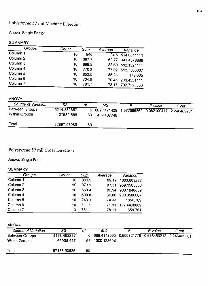
104
Polystyrene 57 mil Machine Direction
Anova: Single Factor
SUMMARY
Groups Count Sum Average VarianceColumn 1 10 946 94.6 514.6511111Column 2 10 697.7 69.77 341.4578889Column 3 10 886.9 88.69 592.1521111Column 4 10 770.2 77.02 512.7506667Column 5 10 852.5 85.25 178.665Column 6 10 704.8 70.48 233.4551111Column 7 10 781.7 78.17 702.7223333
ANOVA
Source of Variation SS
Between Groups
Within Groups
Total
5214.882857
27682.688
32897.57086
df MS P-value F crit
6
63
69
869.1471429
439.407746
1.977996862 0.082100417 2.246409281
Polystyrene 57 mil Cross Direction
Anova: Single Factor
SUMMARY
Groups Count Sum Average Variance
Column 1
Column 2
Column 3
Column 4
Column 5
Column 6
Column 7
10
10
10
10
10
10
10
891.9
873.1
869.4
690.8
743.3
711.1
781.1
89.19
87.31
86.94
69.08
74.33
71.11
78.11
1803.603222
959.1565556
900.1848889
900.0506667
1650.709
127.4498889
659.781
ANOVA
Source of Variation SS df MS P-value F crit
Between Groups
Within Groups
4178.488857 6 696.4148095 0.696321779 0.653460212 2.246409281
63008.417 63 1000.133603
Total 67186.90586 69

105
Polypropylene 50 mil Machine Direction
Anova: Single Factor
SUMMARY
Groups Count Sum Average VarianceColumn 1
Column 2
Column 3
Column 4
Column 5
Column 6
Column 7
10
10
10
10
10
10
10
4396.6
3128.2
3649.7
3478
5245.4
7749.6
4631.5
439.66
312.82
364.97
347.8
524.54
774.96
463.15
74060.216
15977.93956
6061.531222
13731.20444
44662.10933
64340.63822
109514.8206
ANOVA
Source of Variation SS df MS F P-value F crit
Between Groups
Within Groups
Total
1470614.289
2955136.134
4425750.423
6
63
69
245102.3815
46906.92276
5.225292282 0.000202776 2.246409281
Polypropylene 50 mil Cross Direction
Anova: Single Factor
SUMMARY
Groups Count Sum Average Variance
Column 1
Column 2
Column 3
Column 4
Column 5
Column 6
Column 7
10 5572.3 557.23 96144.59344
10 1937.4 193.74 36443.956
10 7405.8 740.58 113653.0729
10 7644.7 764.47 115064.3801
10 4934 493.4 106903.6311
10 6301.6 630.16 148366.6804
10 4519.4 451.94 99841.15378
ANOVA
Source of Variation SS df MS P-value F crit
Between Groups
Wthin Groups
2284877.398 6 380812.8997 3.720861673 0.003137262 2.246409281
6447757.21 63 102345.3525
Total 8732634.608 69

106
Polypropylene 55 mil Machine Direction
Anova: Single Factor
SUMMARY
Groups Count Sum Average VarianceColumn 1
Column 2
Column 3
Column 4
Column 5
Column 6
Column 7
10
10
10
10
10
10
10
3013.5
1907.3
2521.2
2022.6
1649.6
1794.7
1866.9
301.35
190.73
252.12
202.26
164.96
179.47
186.69
4784.376111
6526.335667
34293.73067
6350.311556
978.9804444
2076.749
4075,689889
ANOVA
Source of Variation SS df MS F P-value F crit
Between Groups
Wthin Groups
Total
140459.8794
531775.56
672235.4394
6
63
69
23409.9799
8440.881905
2.773404505 0.018604284 2.246409281
Polypropylene 55 mil Cross Direction
Anova: Single Factor
SUMMARY
Groups Count Sum Average
Column 1
Column 2
Column 3
Column 4
Column 5
Column 6
Column 7
Variance
10 334.1 33.41 90.49655556
10 624.7 62.47 4034.209
10 957.3 95.73 16806.05789
10 666.7 66.67 2973.106778
10 1048.7 104.87 10646.96011
10 390.2 39.02 255.4284444
10 2985 298.5 50548.72
ANOVA
Source of Variation SS df MS P-value F crit
Between Groups
Wthin Groups
501163.1397 6 83527.18995 6.850102221
768194.809 63 12193.5684
1 .25601 E-05 2.246409281
Total 1269357.949 69

107
Elongation (a). Yi^lH ANQVa Results
Polystyrene 52 mil Machine Direction
Anova: Single Factor
SUMMARY
Groups Count Sum Average VarianceColumn 1
Column 2
Column 3
Column 4
Column 5
Column 6
Column 7
10
10
10
10
10
10
10
81.8
80.9
83.4
83.3
83.6
83.5
84.8
8.18
8.09
8.34
8.33
8.36
8.35
8.48
0.019555556
0.014333333
0.231555556
0.040111111
0.020444444
0.113888889
0.099555556
ANOVA
Source of Variation SS df MS F P-value F crit
Between Groups
Wthin Groups
Total
0.993714286
4.855
5.848714286
6
63
69
0.165619048
0.077063492
2.149124614 0.059899314 2.246409281
Polystyrene 52 mil Cross Direction
Anova: Single Factor
SUMMARY
Groups Count Sum Average Variance
Column 1
Column 2
Column 3
Column 4
Column 5
Column 6
Column 7
10 127.3 12.73 10.74455556
10 115.2 11.52 6.608444444
10 120.8 12.08 6.068444444
10 119.9 11.99 5.776555556
10 117.8 11.78 6.526222222
10 114.8 11.48 4.924
10 123.6 12.36 6.538222222
ANOVA
Source of Variation SS df MS P-value F crit
Between Groups
Within Groups
12.17685714 6 2.02947619 0.301068103 0.934077572 2.246409281
424.678 63 6.740920635
Total 436.8548571 69

108
Polystyrene 57 mil Machine Direction
Anova: Single Factor
SUMMARY
Groups Count
10
Sum Average VarianceColumn 1 84.1 8.41 0.098777778Column 2 10 82.6 8.26 0.018222222Column 3 10 83.3 8.33 0.037888889Column 4 10 82.4 8.24 0.064888889Column 5 10 83.2 8.32 0.095111111Column 6 10 85.1 8.51 0.041Column 7 10 83.9 8.39 0.072111111
ANOVA
Source of Variation SS df MS F P-value F critBetween Groups 0.522857143 6 0.087142857 1.425233645 0.219120601 2.246409281Wthin Groups 3.852 63 0.061142857
Total 4.374857143 69
Polystyrene 57 mil Cross Direction
Anova: Single Factor
SUMMARY
Groups Count
Column 1
Column 2
Column 3
Column 4
Column 5
Column 6
Column 7
Sum Average
10 193.6
10 201.5
10 201.2
10 208.7
10 214.2
10 241
10 190.8
Variance
19.36 2.127111111
20.15 1.273888889
20.12 1.635111111
20.87 1.655666667
21.42 0.528444444
24.1 0.037777778
19.08 0.939555556
ANOVA
Source of Variation SS df MS P-value F crit
Between Groups
Wthin Groups
171.6048571 6 28.60080952 24.42260565
73.778 63 1.171079365
9.91647E-15 2.246409281
Total 245.3828571 69

109
Polypropylene 50 mil Machine Direction
Anova: Single Factor
SUMMARY
Groups Count Sum Average VarianceColumn 1
Column 2
Column 3
Column 4
Column 5
Column 6
Column 7
10
10
10
10
10
10
10
188.8
184.5
179.7
183
187.5
189.8
191.1
18.88
18.45
17.97
18.3
18.75
18.98
19.11
0.252888889
0.193888889
0.584555556
0.188888889
0.173888889
0.104
0.085444444
ANOVA
Source of Variation SS df MS F P-value F crit
Between Groups
Wthin Groups
Total
10.06571429
14.252
24.31771429
6
63
69
1.677619048
0.226222222
7.415801291 4.98901 E-06 2.246409281
Polypropylene 50 mil Cross Direction
Anova: Single Factor
SUMMARY
Groups
Column 1
Column 2
Column 3
Column 4
Column 5
Column 6
Column 7
Count Sum Average Variance
10
10
10
10
10
10
10
180.4
179.2
178.1
183.1
179
186.2
189.5
18.04
17.92
17.81
18.31
17.9
18.62
18.95
0.356
0.175111111
0.149888889
0.147666667
0.071111111
0.199555556
0.178333333
ANOVA
Source of Variation SS df MS P-value F crit
Between Groups
Wthin Groups
10.93885714 6 1.823142857 9.988520741 9.88117E-08 2.246409281
11.499 63 0.18252381
Total 22.43785714 69

110
Polypropylene 55 mil Machine Direction
Anova: Single Factor
SUMMARY
Groups Count Sum Average VarianceColumn 1
Column 2
Column 3
Column 4
Column 5
Column 6
Column 7
10
10
10
10
10
10
10
185.2
177.7
182.9
176.1
185.9
189.2
187.8
18.52
17.77
18.29
17.61
18.59
18.92
18.78
0.128444444
0.164555556
0.054333333
0.305444444
0.456555556
0.181777778
0.335111111
ANOVA
Source of Variation SS df MS F P-value F crit
Between Groups
Wthin Groups
Total
14.83771429
14.636
29.47371429
6
63
69
2.472952381
0.23231746
10.64471167 3.88771 E-08 2.246409281
Polypropylene 55 mil Cross Direction
Anova: Single Factor
SUMMARY
Groups Count Sum Average Variance
Column 1
Column 2
Column 3
Column 4
Column 5
Column 6
Column 7
10 166.1 16.61 0.116555556
10 171 17.1 0.18
10 177.8 17.78 0.070666667
10 174.7 17.47 0.264555556
10 174.5 17.45 0.447222222
10 179.8 17.98 0.050666667
10 182.4 18.24 0.020444444
ANOVA
Source of Variation SS df MS P-value F crit
Between Groups
Wthin Groups
18.09485714 6 3.015809524 18.35532799
10.351 63 0.164301587
3.37747E-12 2.246409281
Total 28.44585714 69
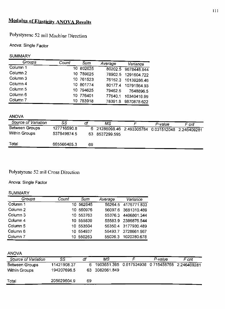
Modulus ofElastirity ANQVA Results
111
Polystyrene 52 mil Machine Direction
Anova: Single Factor
SUMMARY
Groups
Column 1
Column 2
Column 3
Column 4
Column 5
Column 6
Column 7
Count Sum Average Variance
10 802025 80202.5 9678448.944
10 789025 78902.5 1291604.722
10 761523 76152.3 10139286.46
10 801774 80177.4 10791564.93
10 794625 79462.5 7648896.5
10 776401 77640.1 10340416.99
10 783918 78391.8 9870878.622
ANOVA
Source of Variation SS
Between Groups
Wthin Groups
Total
127716590.8
537849874.5
665566465.3
df MS P-value F crit
6
63
69
21286098.46
8537299.595
2.493305784 0.031512048 2.246409281
Polystyrene 52 mil Cross Direction
Anova: Single Factor
SUMMARY
Groups Count Sum Average Variance
Column 1
Column 2
Column 3
Column 4
Column 5
Column 6
Column 7
10 562645 56264.5 4176771.833
10 560976 56097.6 3681310.489
10 553763 55376.3 4406801.344
10 555839 55583.9 2386876.544
10 553504 55350.4 3177930.489
10 554937 55493.7 2728661.567
10 550263 55026.3 1020280.678
ANOVA
Source of Variation SS df MS P-value F crit
Between Groups
Wthin Groups
11421908.37 6 1903651.395 0.617534938 0.715458768 2.246409281
194207696.5 63 3082661.849
Total 205629604.9 69

112
Polystyrene 57 mil Machine Direction
Anova: Single Factor
SUMMARY
Groups Count Sum Average VarianceColumn 1
Column 2
Column 3
Column 4
Column 5
Column 6
Column 7
10
10
10
10
10
10
10
800720
788166
791444
804510
776231
751992
779790
80072
78816.6
79144.4
80451
77623.1
75199.2
77979
12697156.67
8628967.6
4139345.378
14694019.56
10281184.99
11604966.4
5317064.889
ANOVA
Source of Variation SS df MS F P-value F critBetween Groups
Within Groups
Total
187221620.1
606264349.3
793485969.4
6
63
69
31203603.36
9623243.64
3.242524509 0.007686668 2.246409281
Polystyrene 57 mil Cross Direction
Anova: Single Factor
SUMMARY
Groups Count Sum Average
Column 1
Column 2
Column 3
Column 4
Column 5
Column 6
Column 7
Variance
10 506980 50698 617429.3333
10 494223 49422.3 2134078.456
10 498624 49862.4 1716908.044
10 483589 48358.9 1840708.544
10 495698 49569.8 747604.8444
10 489318 48931.8 1209734.4
10 495797 49579.7 697106.9
ANOVA
Source of Variation SS df MS P-value F crit
Between Groups
Within Groups
32079104.29 6 5346517.381 4.175302863 0.001351785 2.246409281
80672134.7 63 1280510.075
Total 112751239 69

113
Polypropylene 50 mil Machine Direction
Anova: Single Factor
SUMMARY
Groups Count
10
10
10
10
10
10
10
Sum
824728
908387
865448
853934
855733
790616
854890
Average
82472.8
90838.7
86544.8
85393.4
85573.3
79061.6
85489
VarianceColumn 1
Column 2
Column 3
Column 4
Column 5
Column 6
Column 7
17512336.18
7408122.233
12621764.84
23020075.6
7167215.567
12668423.6
4906810
ANOVA
Source of Variation
Between Groups
Wthin Groups
Total
SS df MS F P-value F crit
788307770.1
767742732.2
1556050502
6
63
69
131384628.4
12186392.57
10.78125684 3.21206E-08 2.246409281
Polypropylene 50 mil Cross Direction
Anova: Single Factor
SUMMARY
Groups Count
Column 1
Column 2
Column 3
Column 4
Column 5
Column 6
Column 7
Sum Average Variance
10 837514 83751.4 21117970.93
10 848753 84875.3 10769369.57
10 840246 84024.6 6556154.489
10 828352 82835.2 11683075.73
10 817327 81732.7 14016416.46
10 798029 79802.9 2952213.878
10 782211 78221.1 8839054.544
ANOVA
Source of Variation SS df MS P-value F crit
Between Groups 350893068.4 6 58482178.07 5.391180084
Within Groups 683408300.4 63 10847750.8
Total 1034301369 69
0.000151305 2.246409281
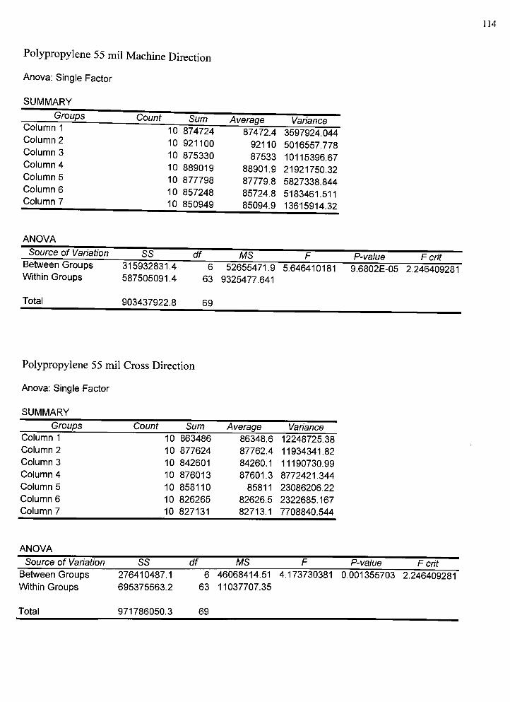
114
Polypropylene 55 mil Machine Direction
Anova: Single Factor
SUMMARY
Groups Count Sum Average VarianceColumn 1
Column 2
Column 3
Column 4
Column 5
Column 6
Column 7
10
10
10
10
10
10
10
874724
921100
875330
889019
877798
857248
850949
87472.4
92110
87533
88901.9
87779.8
85724.8
85094.9
3597924.044
5016557.778
10115396.67
21921750.32
5827338.844
5183461.511
13615914.32
ANOVA
Source of Variation SS df MS F P-value F critBetween Groups
Wthin Groups
Total
315932831.4
587505091.4
903437922.8
6
63
69
52655471.9
9325477.641
5.646410181 9.6802E-05 2.246409281
Polypropylene 55 mil Cross Direction
Anova: Single Factor
SUMMARY
Groups Count Sum Average Variance
Column 1
Column 2
Column 3
Column 4
Column 5
Column 6
Column 7
10 863486 86348.6 12248725.38
10 877624 87762.4 11934341.82
10 842601 84260.1 11190730.99
10 876013 87601.3 8772421.344
10 858110 85811 23086206.22
10 826265 82626.5 2322685.167
10 827131 82713.1 7708840.544
ANOVA
Source of Variation SS df MS P-value F crit
Between Groups
Wthin Groups
276410487.1 6 46068414.51 4.173730381 0.001355703 2.246409281
695375563.2 63 11037707.35
Total 971786050.3 69

115
Appendix F
Critical Values nfF Table
TABLE IV Critical Values ofP
Values ofF00s
Degrees ot freedom tor numerator
T B 9 10 12 60 120
1
2
3
4
5
161 200 216 225 230 234 237 239 241 242 244 246 248 249 250 251 252 253 25418.5
10.1
7.71
6.61
19.0
9.55
6.94
197 197 19.3 19.3 19.4 19.4 19.4 19.4 19.4 19.4 19.4 19.5 19.5 19.5 19.5 19.5 19.59.28 9.12 9.01 8.94 8.89 8.85 8.81 8.79 8.74 8.70 8.66 8.64 8.62 8.59 *S7 8.55 8.536.59 6.39 6.26 6.16 6.09 6.04 6.00 5.96 5.91 5.86 5.80 5.77 5.75 5.72 5.69 5.66 5.63
. 5.79 5.41 5.19 5.05 4.95 4.88 4.82 4.77 4.74 4.68 4.62 4.56 4.53 4.50 4.46 4.43 4.40 4.37
6
7
8
9
10
5.99 5.14 4.76 4.53 4.39 4.28 471 4.15 4.10 4.06 4.00 3.94 3.87 3.84 3.81 3.77 3.74 170 3.675.59 4.74 4.35 4.12 197 3.87 3.79 3.73 168 3.64 3.57 3.51 3.44 -141 3.38 3.34 3.30 377 3735.32
5.12
4.96
4.46 4.07 3.84 169 3.58 3.50 144 3J9 3.35 378 3.22 3.15 3.12 108 3.04 101 197 193476 3.86 3.63 148 3.37 3.29 3.73 118 3.14 3.07 3.01 194 190 186 183 179 175 1714.10 3.71 3.48 133 372 3.14 107 102 198 191 185 177 174 170 166 162 158 154
11
12
13
4.84 3.98 3.59 3.36 370 3.09 101 195 190 185 179 172 165 161 157 153 149 145 1404.75 3.89 149 376 3.11 100 191 185 180 175 169 162 154 151 147 143 138 134 1304.67 3.81 3.41 3.18 103 2.92 183 177 171 167 160 153 146 142 138 134 130 125 121
. 14 4:60 .3.74 3.34 3.11 2.96 185 176 170 165 160 153 146 139 135 131 277 122 118 11315 4.54 3.8 379 3.06 2.90 2.79 171 164 159 154 148 140 133 279 125 270 116 111 107
16 4.49 3.63 374 3.01 2.85 2.74 166 159 154 149 142 135 278 124 119 115 111 106 101n 4.45 3.59 370 2.96 781 2.70 161 155 149 145 138 131 273 279 115 110 106 101 1.9618 - 4.41 3.55 3.16 2.93 2.77 2.66 158 151 146 141 134 127 119 115 111 106 102 1.97 1.9219 4.38 3.52 3.13 2.90 2.74 2.63 154 148 142 138 131 123 116 111 107 103 1.98 1.93 1.8820 4J5 3.49 3.10 2.87 2.71 160 151 145 139 135 278 270 112 108 104 1.99 1.95 1.90 1.84
21 4.32 3.47 3.07 2.84 2-68 757 149 142 137 132 125 118 110 105 101 1.96 1.92 1.87 1.8122 4J0 3.44 3.05 2.82 2.66 2.55 146 140 134 130 123 115 107 103 1.98 1.94 1.89 1.84 1.7823 478 3.42 3.03 2.80 2.64 153 144 137 2J2 277 270 113 105 101 1.96 1.91 1.86 1.81 1.7624 476 3.40 101 2.78 2.62 151 142 136 130 275 118 111 103 1.98 1.94 1.89 1.84 1.79 1.7325 474 139 2.99 2.76 2.60 149 140 134 128 274 116 109 101 1.96 1.92 1.87 1.82 1.77 1.71
30 4.17 3J2 192 2.69 2.53 142 133 127 271 116 109 101 1.93 1.89 1.84 1.79 1.74 1.68 1.62
40 4.08 373 184 2.61 2.45 134 125 118 112 108 100 1.92 1.84 1.79 1.74 1.69 1.64 1.58 1.51
60 4.00 3.15 2.76 2.53 131 275 117 110 104 1.99 1.92 1.84 1.75 1.70 1.65 1.59 1.53 1.47 U9120 3.92 3.07 2.68 2.45 279 2.18 109 102 1.96 1.91 1.83 1.75 1.66 1.61 1.55 1.50 1.43 1.35 175CO 3.14 3.00 2.60 137 271 110 101 1.94 1.88 1.83 1.75 1.67 1J7 1.52 1.46 1.39 U2 172 1.00
' Reproduced from M. MerrinftonudCM. Thompson,Tiblel ofpercentage points ofthe inverted beU (F)distribution,"
Bumtlrlka, voL 33 (1943), by permission of the Biomctrika trustees.
(Freund, John E. and Gary A. Simon, 529)


