Download - Meditations Meditations On Basic Open Hole Log Validation Techniques Revised: June 1998.

Meditations Meditations On

Basic Open Hole Log Validation Techniques

Revised: June 1998

2

Meditations Meditations On

Basic Open Hole Log Validation Techniques

Schlumberger Field Engineers are currently witnessing significant changes in wireline technology. The toolstrings are shorter, lighter, more integrated, and more combinable. The hardware is more reliable and the processing is playing an increasingly important role. The industry is also demanding improved efficiency.

The result is we are logging more sensors in less time. The tasks our Field Engineers are required to perform have changed, but they haven’t decreased in number or become less demanding. And the techniques that our Field Engineers use to validate the logs they deliver the client have not evolved with the technology.

The objective of this package is to provide you, the Field Engineer, with the techniques necessary to validate the PLATFORM EXPRESS - BHC Sonic Logs you deliver the client.

This package will cover Master Calibrations, Before Calibrations, Log Response, LQC Formats, Repeatability, Offset Logs, Depth, Parameter Validation, and Presentation.

I hope it helps. Good luck!

Bruce Townson

3

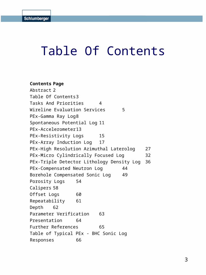
Table Of Contents

Contents Page

Abstract 2

Table Of Contents 3

Tasks And Priorities 4

Wireline Evaluation Services 5

PEx-Gamma Ray Log 8

Spontaneous Potential Log 11

PEx-Accelerometer 13

PEx-Resistivity Logs 15

PEx-Array Induction Log 17

PEx-High Resolution Azimuthal Laterolog 27

PEx-Micro Cylindrically Focused Log 32

PEx-Triple Detector Lithology Density Log 36

PEx-Compensated Neutron Log 44

Borehole Compensated Sonic Log 49

Porosity Logs 54

Calipers 58

Offset Logs 60

Repeatability 61

Depth 62

Parameter Verification 63

Presentation 64

Further References 65

Table of Typical PEx - BHC Sonic Log

Responses 66

4

Tasks and Priorities

As a Field Engineer on location, you usually have oodles of tasks to accomplish. You can complete some of them through multitasking while others require 100% of your attention. Most of the time you will prioritize these tasks in order of importance and address them accordingly.

The typical priorities of a Field Engineer are, in chronological order:

1. To Acquire Quality Data.

2. To Process Quality Answers.

3. To Present Quality Logs.

4. To Deliver Quality Products.

Each of these priorities are equally important, however without quality data, you can not process quality answers. Without quality answers, you can not present quality logs. And without quality logs, you can not deliver quality products. This is why you start with Priority 1and work down the list.

Consider when your busiest time is during logging. It is probably when you are logging off bottom. There are logs to watch, headers to complete, formats to annotate, data channels to set up, fax copies to deliver the client, and overspeed aborting to watch, just to name a few of the tasks that are usually completed during this time.

Now consider when you are logging the most important interval of the well. It is probably when you are logging off bottom, which coincides with the busiest time during logging. Some of the tasks you are accomplishing have to do with Log Presentation and Product Delivery. The tasks you should be concentrating on most at this point should be Data Acquisition and Answer Processing.

As you step through this training package, please keep in mind the order of priorities listed above. Hopefully it will help you develop techniques of your own that will improve the quality of your logs.

5

Wireline Evaluation Services

The primary purpose of running basic open hole logs is to provide petrophysical evaluation of subsurface formations. Our clients want to know how much oil and/or gas is downhole. Unfortunately, our sensors don’t provide the information necessary to determine this volume of hydrocarbons directly. Our sensors do, however, provide the information necessary to determine the volume of water downhole, from which the volume of hydrocarbons can be inferred.

Following below is an explanation of how this is done.

First, we assume that formation pore space is filled with either water, oil, or gas.

Next, we define some terms:

Sw= the percentage of formation pore space by volume that is filled with water; and,

Shc= the percentage of formation pore space by volume that is filled with hydrocarbons (i.e. oil and gas).

Therefore:

Sw + Shc = 1.

6

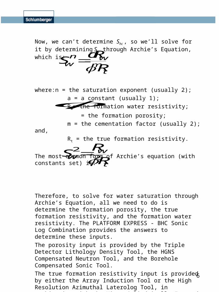
Now, we can’t determine Shc , so we’ll solve for it by determining Sw through Archie’s Equation, which is:

where:n = the saturation exponent (usually 2);

a = a constant (usually 1);

Rw= the formation water resistivity;

= the formation porosity;

m = the cementation factor (usually 2); and,

Rt = the true formation resistivity.

The most common form of Archie’s equation (with constants set) is:

Therefore, to solve for water saturation through Archie’s Equation, all we need to do is determine the formation porosity, the true formation resistivity, and the formation water resistivity. The PLATFORM EXPRESS - BHC Sonic Log Combination provides the answers to determine these inputs.

The porosity input is provided by the Triple Detector Lithology Density Tool, the HGNS Compensated Neutron Tool, and the Borehole Compensated Sonic Tool.

The true formation resistivity input is provided by either the Array Induction Tool or the High Resolution Azimuthal Laterolog Tool, in combination with the Micro Cylindrically Focused Logging Tool.

And the formation water resistivity is provided by an analysis of the entire PLATFORM EXPRESS - BHC Sonic Log Conbination using the Rwa Method, by an SP log analysis using the SP Method, by MDT/RFT sample measurement, or by reference to the Formation Water Resistivity Tables.

SaR

Rwn w

mt

S

R

Rww

t

22

7

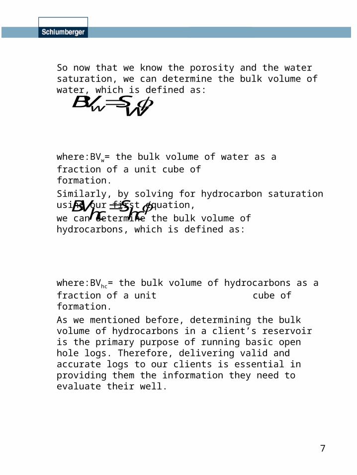
So now that we know the porosity and the water saturation, we can determine the bulk volume of water, which is defined as:

where:BVw= the bulk volume of water as a fraction of a unit cube of formation.

Similarly, by solving for hydrocarbon saturation using our first equation,

we can determine the bulk volume of hydrocarbons, which is defined as:

where:BVhc= the bulk volume of hydrocarbons as a fraction of a unit cube of formation.

As we mentioned before, determining the bulk volume of hydrocarbons in a client’s reservoir is the primary purpose of running basic open hole logs. Therefore, delivering valid and accurate logs to our clients is essential in providing them the information they need to evaluate their well.

BV Sww

BVhc Shc

8

PEx - Gamma Ray Log

Applications.The Gamma Ray Log is used for:

•correlating between descents and trips to the well;•correlating between open hole logs and cased hole logs;•indicating formation shale content;•identifying formation tops; and,•detecting radioactive and non-radioactive minerals.

The PEx GR can be run in any combination of air-filled, fresh , salty, or oil-based muds and open or cased hole conditions.

Master Calibrations.There are no Master Calibrations for the PEx-GR.

Before Calibrations.The Before Calibrations consist of a two point calibration which computes a gain that is applied to the raw GR count rate. The first (or zero) calibration measurement is a background GR activity reading. The second (or plus) calibration measurement is a reading taken with a calibration jig (a.k.a. blanket) which determines the combined GR activity of the background and jig. The gain applied to the raw GR count rate is computed as follows:

Gain = _____Jig Value_____

PlusMeas - ZeroMeas

where:Jig Value = 160 GAPI for GSR-Ys and different for each GSR-U;

PlusMeas = background GR activity + jig GR activity; and,

ZeroMeas = background GR activity.

9

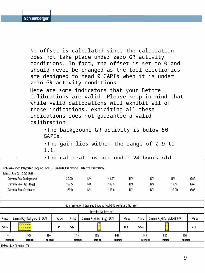
No offset is calculated since the calibration does not take place under zero GR activity conditions. In fact, the offset is set to 0 and should never be changed as the tool electronics are designed to read 0 GAPIs when it is under zero GR activity conditions.

Here are some indicators that your Before Calibrations are valid. Please keep in mind that while valid calibrations will exhibit all of these indications, exhibiting all these indications does not guarantee a valid calibration.

•The background GR activity is below 50 GAPIs.•The gain lies within the range of 0.9 to 1.1.•The calibrations are under 24 hours old when logging operations begin.

Here’s an example CSL from what could be a good calibration.

10

Log Response.The PEx-GR measures the amount of naturally occuring radioactivity in the formation.

The PEx-GR has two vertical resolutions: the GR output which uses a 6” sampling rate; and the HGR output which uses a 2” sampling rate. The PEx-GR can be run at 3600 fph (18m/min) for standard resolution (GR) and 1800 fph (9m/min) for high resolution (HGR).

A clean formation is a formation free of shale. Clean formations usually have low GR activity while shales have high GR activity. Therefore formations that contain shale will have higher GR readings than clean formations. Formations may also have high GR readings if they contain radioactive minerals.

The PEx-GR log can be affected by:•tool eccentering;•the barite content of the mud; and,•tool standoff.

Please see the Table of Typical PEx - BHC Sonic Log Responses on page 66.

LQC Format. The HILTIndLQC and HILTLatLQC formats each contain two curves that relate to the PEx-GR: GR and CFGR.

•GR is the output that was discussed in the Log Response section. •CFGR is the GR Borehole Correction Factor that is applied to the GR output to compensate for eccentering, barite in the mud, and standoff. CFGR should lie between 0.8 and 1.2.

Repeatability.The GR output should repeat within 7% of itself.

11

Spontaneous Potential Log

Applications.The Spontaneous Potential Log (a.k.a. SP) is used for:

•correlating between descents and trips to the well;

•detecting permeable beds;

•identifying bed boundaries;

•determining Rw; and,

•indicating formation shale content.

The SP can only be run in conductive (ie. fresh or salty) mud systems in open hole.

Master and Before Calibrations.There are no Master or Before Calibrations for the SP.

Pre-Logging Check.The SP log requires line 8 to be grounded to earth. The SP Pre-Logging Check consists of checking the SP voltage return on line 8 while logging. This is done by starting a log, holding the SP Return Test button down on the SSD (MBM, DBM) and watching the SP output on the log or I/O Monitor (the SP Return Test on the WFDD (MCM) is not currently operational). The SP Return Test sends current down line 8. If line 8 is grounded, this current will dissipate into the ground and the SP will not be affected. However, if line 8 is not properly grounded, the current will result in a charge buildup along line 8 which will create a natural capacitor (lines 7 and 8 act as the electrodes while the formation acts as the insulator) and the SP output will wrap.

Please note that this test is not relevant if you are using AHSCA, the AITH’s digital SP.

12

Log Response.The SP is a measurement of the voltage potential created from ion movement caused by the effects of the drilling process.

The SP is defined with a baseline in shales which have no invasion, and with deflections in formations which have invasion.

Here are some factors that affect the SP log.•As a formation bed thickness increases, the deflection increases.•As a formation shale content increases, the deflection decreases.

•The relative resistivities of Rmf and Rw will determine whether the SP deflection is positive or negative ( in Western Canada Rmf > Rw almost all of the time).

–If Rmf > Rw , then the deflection is negative.

–If Rmf < Rw , then the deflection is positive.

–If Rmf = Rw , then there is no deflection.

The SP is a smooth curve, therefore there should be no spikes.

If an SP baseline shift needs to be made, this should be done in a shale and not in a zone of interest.

There are no logging speed restrictions for the SP.

Please see the Table of Typical Pex - BHC Sonic Log Responses on page 66.

LQC Format.There are no SP related curves on the HILTIndLQC or HILTLatLQC formats.

Repeatability.The SP should repeat within 2 mV after the allowance for a baseline shift since the reading values are relative and not absolute.

13

PEx-AccelerometerApplications.

The PEx-Accelerometer is used for:

•speed correction ; and,

•deviation information.

The PEx-Accelerometer can be used in all deviated and vertical borehole conditions.

Master Calibrations.There are no Master Calibrations for the PEx-Accelerometer.

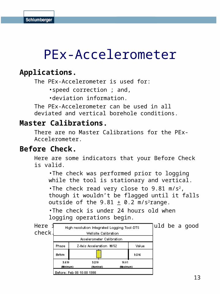
Before Check.Here are some indicators that your Before Check is valid.

•The check was performed prior to logging while the tool is stationary and vertical.

•The check read very close to 9.81 m/s2, though it wouldn’t be flagged until it falls outside of the 9.81 + 0.2 m/s2range.

•The check is under 24 hours old when logging operations begin.

Here is an example CSL from what could be a good check.

14

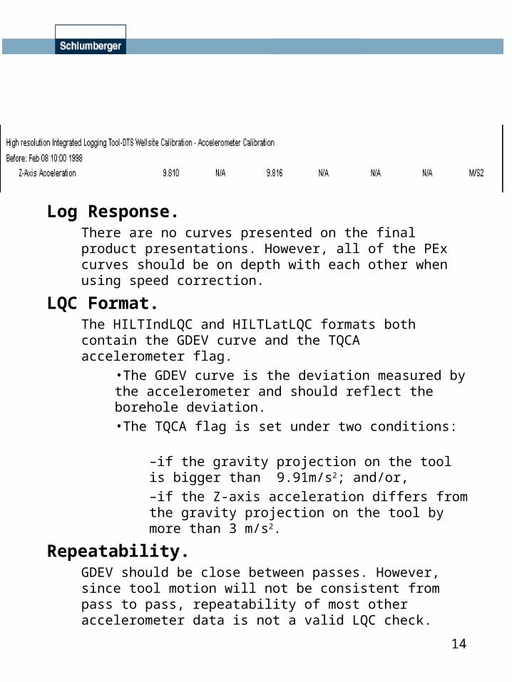
Log Response.There are no curves presented on the final product presentations. However, all of the PEx curves should be on depth with each other when using speed correction.

LQC Format.The HILTIndLQC and HILTLatLQC formats both contain the GDEV curve and the TQCA accelerometer flag.

•The GDEV curve is the deviation measured by the accelerometer and should reflect the borehole deviation. •The TQCA flag is set under two conditions:

–if the gravity projection on the tool is bigger than 9.91m/s2; and/or,–if the Z-axis acceleration differs from the gravity projection on the tool by more than 3 m/s2.

Repeatability.GDEV should be close between passes. However, since tool motion will not be consistent from pass to pass, repeatability of most other accelerometer data is not a valid LQC check.

15

PEx - Resistivity Logs

The PLATFORM EXPRESS offers two different Resistivity Logs: an Array Induction Log and a High Resolution Azimuthal Laterolog. Both of these logs are used for the same applications, however they each have their own operating environments. Only one of these Resistivity tools can be run at any time since they are both bottom only tools.

This section is intended to discuss the applications of these tools and how to determine which one to run under specific operating conditions.

Applications.The PEx-AITH and PEx-HALS tools are both designed for:

•determining Rt;

•evaluating Sw;

•analyzing drilling fluid invasion;

•identifying permeability; and,

•correlating.

In addition, through it’s azimuthal measurements, the PEx-HALS can be used for:

•evaluating horizontal and or highly deviated wells;

•evaluating heterogeneous formations; and,

•analyzing fractures.

Operating Environments.The PEx-AITH is an array induction tool which induces ground loops in the formation and measures conductivity. Therefore, it is suited for:

•lower resistivity (higher conductivity) formations;

•vertical wells with formations that are laid in horizontal planes;

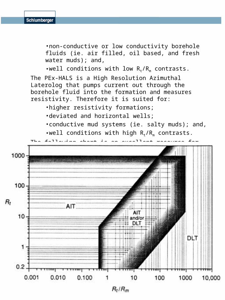
16

•non-conductive or low conductivity borehole fluids (ie. air filled, oil based, and fresh water muds); and,

•well conditions with low Rt/Rm contrasts.

The PEx-HALS is a High Resolution Azimuthal Laterolog that pumps current out through the borehole fluid into the formation and measures resistivity. Therefore it is suited for:

•higher resistivity formations;•deviated and horizontal wells;•conductive mud systems (ie. salty muds); and,

•well conditions with high Rt/Rm contrasts.

The following chart is an excellent resource for helping you determine which tool to run under specific operating conditions (please replace HALS for DLT in this graph).

17

PEx - Array Induction Log

Please see the section on PEx - Resistivity Logs for the applications of the PEx-AITH.

Master Calibrations.To summarize, the Master Calibrations for the PEx - AITH consist of determining the magnitude gain and offset to apply to each receiver coil, the phase shift to apply to each receiver coil, and the gain to apply to the the mud sensor measurements.

Temperature Coefficients.

The first Master Calibration step is to retrieve, by GET, EEPROM read, or entering them by hand, the Array Temperature Coefficients that were characterized in Houston. These coefficients correct the individual receiver measurements for conductivity variations due to receiver temperature. If the calibrations are performed without these coefficients, then the measurements are invalid, as are the calibrations. Please note that characterizing the array receivers is done once in a sonde’s life unless the array has been dismantled or any array components have been replaced, at which point the sonde must be recharacterized in Houston.

Test Loop Gain and Phase Measurements.

The second step is the Test Loop Gain and Phase Measurements. A measurement is taken for all receivers which determines the combined background and inherent sonde conductivity. Following this are eight more measurements, one for each of the receivers where a conductive test loop of known resistance is placed around the sonde. These measurements determine the combined background, inherent sonde, and test loop conductivity. Here is how the gain for each receiver is calculated:

18

Gain =__Test Loop Value__

PlusMeas - ZeroMeas

where: Test Loop Value = known conductivity of the test loop used for that receiver;

PlusMeas = combined conductivity of the background, sonde, and test loop

measured by that receiver; and,

ZeroMeas = combined conductivity of the background and sonde measured

by that receiver.

During the plus measurement, the phase shift applied to the receiver measurement is determined as followed:

PS = Pmodel - Pmeasured

where: PS = Phase Shift applied to that receiver;

Pmodel = model phase known for that receiver; and,

Pmeasured = measured phase determined for that receiver.

Sonde Error Corrections.

The third calibration step is the determination of the Sonde Error Corrections. This is the receiver offset value.The Sonde Error Corrections subtract the component of the conductivity that is seen by each receiver that is due to the inherent conductivity of the sonde. This is done by taking a measurement of the combined background and sonde conductivity 4’ off the ground and another measurement at 12’ off the ground. In both of these measurements the sonde conductivity component will be the same. However, the background conductivity component will decrease as the sonde is moved from 4’ off the ground to 12’ off the ground. The correction is made for both the X and R signals of all 8 receivers, making 16 corrections in total, by using a non-linear extrapolation to a position infinitely far away where the background is eliminated and only the sonde conductivity component is left.

19

Mud Sensor Gains.

The third and final master calibration step is to calibrate the mud sensor. This measurement is a one point calibration that assumes an offset of zero and determines a coarse gain and a fine gain applied in the determination of the Rm output.

Here are some indicators that your PEx-AITH Master Calibrations are valid.

•0.95 < GAIN < 1.05.•-3 < PS< 3.•Sonde Error Corrections are within individual limits.•The Coarse and Fine Mud Gains are within the 0.6 to 1.4 limits, although in reality the gains are usually 1.0 to 1.2.•All PEx-AITH Master Calibrations are less than 3 months old.

Before Checks.There are three checks that can be performed: the Electronics Calibration Check that checks the operation of the preamplifiers in the cartridge; the Electronics Zero Check that checks for crosstalk in the A-D converters in the cartridge; and the Array Calibration Check that checks the operation of the receivers in a zero conductivity area. Since there are no zero conductivity areas at the wellsite, the Array Calibration Check is not performed.

Here are some indicators that your Electronics Calibration Check and Electronics Zero Check are valid.

•The checks were performed within 24 hours of starting logging operations.• The Electronics Zero and Calibration Check measurements are all within limits.

20

Here’s an example of an Electronics Calibration Check that could be valid.

21

Logging Response:The PEx-AITH measures the conductivity of the formation and borehole fluid. Conductivity must, by definition, be positive. Conductivity is also the inverse of resistivity and can be related to resistivity by the following equation:

R = 1000

C

where: R = resistivity in ohm metres; and,

C = conductivity in milli mhos/ metre.

Since the resistivity curves are usually displayed on a logarithmic scale from 0.2 to 2000 ohm m, it is hard to see if the resistivities are ever below zero since all you can see is a drop below 0.2 ohm m. However the conductivity curve on the linear 1:600 presentation is scaled from 0 to 1000 mm/m and you can easily identify if the conductivity is negative. You should watch for negative conductivity since it happens frequently. It’s usually a sign of a bad master calibration where a sonde error correction (a.k.a. receiver conductivity offset) was improperly calculated. Sonde error corrections can easily be as large as -100 mm/m, which, using the formula above, is equivalent to -10 ohm m.

22

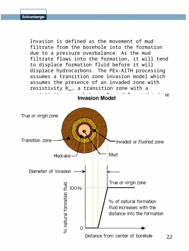
Invasion is defined as the movement of mud filtrate from the borehole into the formation due to a pressure overbalance. As the mud filtrate flows into the formation, it will tend to displace formation fluid before it will displace hydrocarbons. The PEx-AITH processing assumes a transition zone invasion model which assumes the presence of an invaded zone with resistivity Rxo, a transition zone with a resistivity range between Rxo and Rt , and a true zone with resistivity Rt.

23

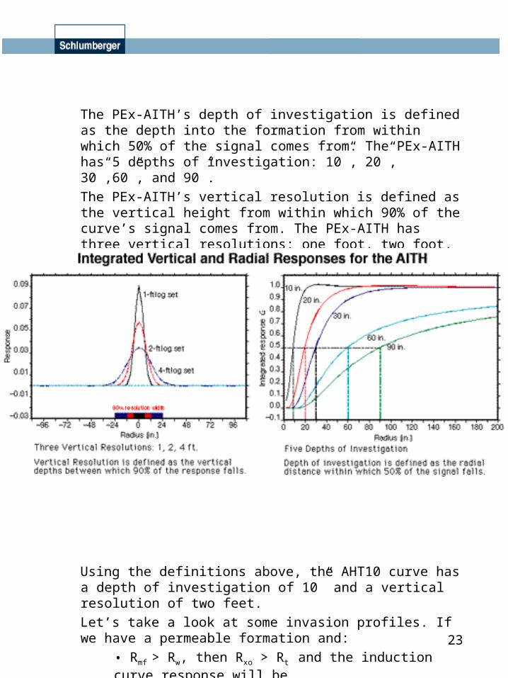
The PEx-AITH’s depth of investigation is defined as the depth into the formation from within which 50% of the signal comes from. The PEx-AITH has 5 depths of investigation: 10”, 20”, 30”,60”, and 90”.

The PEx-AITH’s vertical resolution is defined as the vertical height from within which 90% of the curve’s signal comes from. The PEx-AITH has three vertical resolutions: one foot, two foot, and four foot. The smaller the vertical resolution the better since pay zones can be as thin as a metre. However, the shorter vertical resolutions are less robust to borehole effects than the taller ones.

Using the definitions above, the AHT10 curve has a depth of investigation of 10” and a vertical resolution of two feet.

Let’s take a look at some invasion profiles. If we have a permeable formation and:

• Rmf > Rw, then Rxo > Rt and the induction curve response will be AHT10>AHT20>AHT30>AHT60>AHT90;

•Rw > Rmf, then Rt > Rxo and the induction curve response will be AHT90>AHT60>AHT30>AHT20>AHT10; or,

• Rw = Rmf, then Rt = Rxo and the induction curve response will be AHT10=AHT20=AHT30=AHT60=AHT90.

24

If we have an impermeable formation (ie. shale):•then there will be no invasion and the curves will overlay: AHT10=AHT20=AHT30=AHT60=AHT90.

The preceding examples hold true for the one and four foot resolutions as well as the two foot resolution represented.

In most instances, the mud filtrate does not invade past 60” into the formation, so the AHT90 curve can be assumed to be Rt.

Here are some indicators of a valid log:•the borehole and formation conditions fall under the PEx-AITH’s operating conditions; •the conductivity output (ie. AHTCO90) is positive;•the 10” curve tracks the RXOZ curve;•the curves follow one of the invasion profiles; •the caliper input is working and the borehole is gauge and smaller than 305 mm; and,•the logging speed is 3600fph (18 m/min) or less.

Please see the Table of Typical PEx - BHC Sonic Log Responses on page 66.

LQC Format.There are five flags and twelve curves on the HILTIndLQC format to help determine whether the log is valid or not.

•The HAIT Hardware Flag is itself a summary of the AHDES AITH Diagnostic Executive Summary you find in the I/O Monitor. It is yellow if any of the following bits are set: Diag Tool State; Diag SPA; or Ind Raw Gain Orng. It is red if any of the following bits are set: Diag Temp; Diag Volt; Diag Ind Thru Cal Dif; Diag Ind Thru Cal Rng; Tool Status Low; Tool Status High. If the Hardware Flag is yellow or red, chances are you have a serious hardware failure.•The AHMF curve is the mud resistivity measured by the Rm sensor. This resistivity should compare with the mud resistivity recorded on surface after temperature has been taken into account (a temperature increase causes a resistivity decrease).

25

•The AHTCA is the PEx-AITH temperature output that is used in applying the temperature coefficient corrections to the receiver conductivity signals. Though this temperature reflects the temperature of the thermally insulated receivers, it should still compare to HTEM and the expected borehole temperature.•The eight PEx-AITH Quality Control Fully Calibrated Signals (AHQAB[0-7]) from the eight receivers are all calibrated, depth matched, and borehole corrected. They are presented as conductivities and they should all overlay well except when borehole effects are sgnificant.•The four HAIT Array Flags look at the Quality Control Fully Calibrated Signals. Each array has an associated Quality Control Ratio which is defined as the ratio of two subsequent elements of the Quality Control Fully Calibrated Signals. The flags are conditions of 2 ratios as given below with the ratio definitions:

–HAIT Array[1,2]•AHQRI[0] = AHQAB[1]/AHQAB[0]•AHQRI[1] = AHQAB[2]/AHQAB[1]



–HAIT Array[7,8]•AHQRI[6] = AHQAB[6]/AHQAB[6] This ratio is always 1 and therefore always green.•AHQRI[7] = AHQAB[7]/AHQAB[6].

The flags are yellow if the corresponding AHQRI is >1.5 which indicates a malfunctioning array or a deficiency in the borehole correction.

26

•The last curve is the PEx-AITH Borehole/Formation Signal Ratio (AHBFR) which is an indication of how much the processing is depending on the input parameters to correct for the borehole signal. An AHBFR value below 1.375 indicates that the parameter inputs are not that important, while a value between 1.375 and 2.25 indicates they are important, and a value above 2.25 indicates that they are critical. The higher the AHBFR value, the more accurate your parameter inputs need to be.

Repeatability.The AHT10, AHT20, AHT30, AHT60, and AHT90 induction curves should all repeat within 2% up to 25 ohm m. Above 25 ohm m, the repeatability deteriorates to + 7 ohm m at 100 ohm m and + 300 ohm m at 500 ohm m. Meanwhile the Rm Sensor output AHMF should repeat within 5% from 0.05 to 5 ohm m.

27

PEx - High Resolution Azimuthal Laterolog

Please see the section on PEx - Resistivity Logs for the applications of the PEx-HALS.

Master Calibrations.There are no Master Calibrations for the PEx-HALS.

Before Calibrations.The Before Calibrations consist of gain and phase corrections to the electronic components. The calibration is performed by connecting the preamplifiers to a small network of reference resistors through a set of switches. A measurement is taken without an applied current and another one taken with an applied current.

Here is how the gain for each component is calculated:

Gain =Ref. Resistor Value

PlusMeas - ZeroMeas

where: Ref. Resistor Value = resistance of the reference resistor used for that component;

PlusMeas = resistance measured by the component when a current is applied; and,

ZeroMeas = resistance measured by the component when a current is not applied.

28

During the plus measurement, the phase shift applied to the receiver measurement is determined as followed:

PS = Pmodel - Pmeasured

where: PS = Phase Shift applied to that component;

Pmodel = model phase known for that component;and,

Pmeasured = measured phase determined for that component.

Here are some indicators of a valid Before Calibration.•The gains are very close to 1, usually within 0.02 (see the CSL for the exact limits for each measurement).•The phases are very close to 0, usually within 1 (see the CSL for the exact limits for each measurement).•The calibrations are under 24 hours old when logging operations begin.

An example CSL has not been included because it is so long!!!!

Log Response.The PEx-HALS outputs provide two vertical resolutions, two depths of investigation, and azimuthal profiling. The HLLD and HLLS standard outputs have a vertical resolution of 16”, while the HRLD and HRLS high resolution outputs have a vertical resolution of 8”. Unlike the PEx-AITH, the PEx-HALS does not provide outputs with fixed depths of investigation. The HLLD and HRLD deep curves have a depth of investigation of about 60” which decreases as the R t/Rm contrast becomes smaller. The HLLS and HRLS shallow curves have a depth of investigation of about 30” which decreases as the R t/Rm contrast becomes smaller as well.

The PEx-MCFL is usually run with the PEx-HALS to provide a third resistivity output, RXOZ or RXO8 or RXOI, with a shallower depth of investigation. This third resistivity output simplifies the invasion profiling necessary to determine Rt.

The PEx-HALS uses the step profile invasion model where the mud filtrate is assumed to invade to a certain depth at which point there is an abrupt transition where the formation fluid is then assumed to be contained in the pore spaces.

29

Though not usually presented, HART is the computed Rt which comes from taking the PEx-HALS and PEx-MCFL inputs and putting them through a tornado chart computation (this tornado chart can be found on page 8-49 of the HILT-B Field Engineer’s Manual if you’re interested).

Let’s take a look at some invasion profiles. If we have a permeable formation and:

• Rmf > Rw, then Rxo > Rt and the resistivity curve response will be RXOZ>HLLS>HLLD;

•Rw > Rmf, then Rt > Rxo and the resistivity curve response will be HLLD>HLLS>RXOZ; or,

• Rw = Rmf, then Rt = Rxo and the resistivity curve response will be RXOZ=HLLS=HLLD.

If we have an impermeable formation (ie. shale):•then there will be no invasion and the curves will overlay: RXOZ=HLLS=HLLD.

Of course, the above holds true for high resolution curves as well.

Please see the Table of Typical PEx- BHC Sonic Log Responses on page 66.

Here are some indicators that you have a valid log.•The borehole and formation conditions fall under the PEx-HALS’ operating conditions.

•Rm < 5 ohm m.

•The electrical stand-off conductivity curves overlay when the tool is centralized.•The curves follow one of the invasion profiles.•The deep and shallow azimuthal resistivity curves may spike in fractured formations.•The ZBA1, ZBA2, and ZBA3 bucking attenuation signals that you can connect in the I/O Monitor should fluctuate between 0 dB and 90 dB. If the signals read a constant 90 dB that means that mode is saturated and the readings will be meaningless for that mode.•The logging speed is 3600fph (18 m/min) or less.

30

LQC Format.There are four curves and three flags on the HILTLatLQC format to help you validate your PEx-HALS log.

•The HALS Hardware flag (QCHALS) is triggered if the auxiliary loops are malfunctioning, if the vertical mode loop malfunctions, if there is excessive noise in the monitoring voltages, if the voltage or current amplitudes exceed the signal handling capacity of the hardware and/or software, if the instrumentation is contributing too much noise, or if Groningen conditions have been detected.•The HALS Processing (HLLD) flag is triggered if any of the following conditions are met:

–HLLD > 100,000 ohm m;

–Rt/Rm < 1; and,

–HLLD Groningen correction coefficient < 0.6.•The HALS Processing (HLLS) flag is triggered if any of the following conditions are met:

–HLLS > 100,000 ohm m;

–Rt/Rm < 1; and,

–HLLS borehole correction coefficient > 1.4.•The CCHLLD and CCHLLS standard resolution correction factors indicate the amount of correction applied to the raw HLLD and HLLS curves respectively. If these curves fall outside the 0.8 to 1.2 range, the log may be invalid in those areas.•The CCHRLD and CCHRLS high resolution correction factors indicate the amount of correction applied to the raw HRLD and HRLS curves respectively. If these curves fall outside the 0.8 to 1.2 range, the log may be invalid in those areas.

31

Repeatability.The PEx-HALS HLLD, HLLS, HRLD, and HRLS curves should repeat within the following tolerances:

•+ 10% when the resistivity lies between 0.2 and 1 ohm m;•+ 5% when the resistivity lies between 1 and 2000 ohm m;•+ 10% when the resistivity lies between 2000 and 5000 ohm m; and,•+ 20% when the resistivity lies between 5000 and 40000 ohm m.

Since it is sensitive to the relative bearing of the tool, a specific azimuthal resistivity output may not repeat a spike caused by a fractured formation though another azimuthal resistivity output should pick it up.

32

PEx - Micro Cylindrically Focused Log

Applications.The PEx-MCFL Log is used for:

•measuring Rxo to help determine Rt;

•detecting mudcake to identify permeable beds;

•measuring mudcake to make borehole correction algorithms for devices such as the PEx-TLD;

•identifying fractures; and,

•evaluating sand-shale laminations.

The PEx-MCFL can be run in all conductive borehole fluids, but not in air filled holes or oil based mud systems.

Master Calibrations.There are no Master Calibrations for the PEx-MCFL.

Before Calibrations.The Before Calibrations consist of a series of internal electronics calibrations using precision resistors in the skid as references.

Here are some indicators that your calibrations are valid.

•The measured voltages, currents, and resistances fall within the acceptable ranges.

•The B0, B1, and B2 Resistivity gains are all very close to 1 (they’re usually between 0.98 to 1.02).

•The calibrations are under 24 hours old when logging operations begin.

33

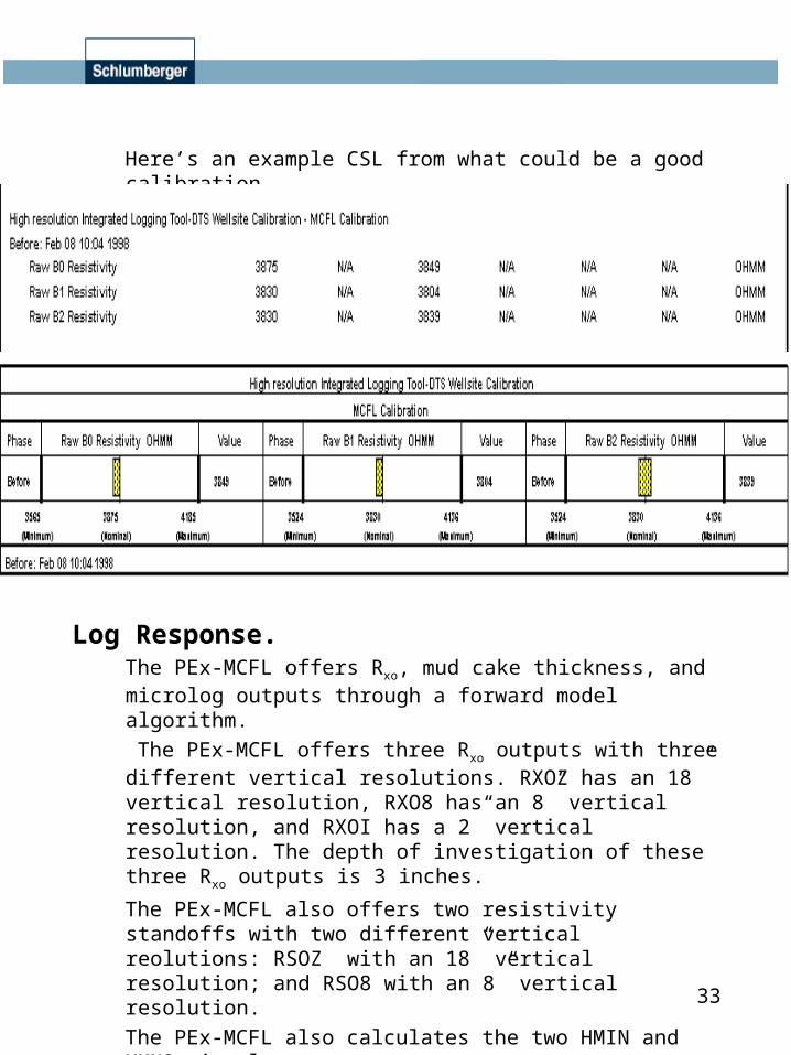
Here’s an example CSL from what could be a good calibration.

Log Response.The PEx-MCFL offers Rxo, mud cake thickness, and microlog outputs through a forward model algorithm.

The PEx-MCFL offers three Rxo outputs with three different vertical resolutions. RXOZ has an 18” vertical resolution, RXO8 has an 8” vertical resolution, and RXOI has a 2” vertical resolution. The depth of investigation of these three Rxo outputs is 3 inches.

The PEx-MCFL also offers two resistivity standoffs with two different vertical reolutions: RSOZ with an 18” vertical resolution; and RSO8 with an 8” vertical resolution.

The PEx-MCFL also calculates the two HMIN and HMNO microlog outputs.

34

Here are some indicators that these logs are valid.•The borehole fluid is conductive (ie. not oil based muds or air).•The logging environment falls within the following forward model operating limits:

– 0.2 ohm m < Rxo < 2000 ohm m;

– 0.02 ohm m < Rmc < 2 ohm m;

– 3 < Rxo/Rmc < 10,000;

– Rxo/Rmc2 < 80,000 S/m; and,

– 0 < hmc (ie. mud cake thickness) < 20 mm.•RXOZ compares well with the PEx-AITH 10” induction curves and the PEx-HALS HRLS and HLLS resistivity curves.•RSOZ:

–agrees with the PEx-TLD’s DSOZ output;– is 0 mm in sections of smooth borehole and no mudcake;

and,– is less than 20 mm.

•HMIN and HMNO overlay in zones with no mudcake. Though HMIN and HMNO are resistivity readings, they are qualitative and not absolute.•HMNO is larger than HMIN when there is mudcake.•The HCAL caliper shows a smooth borehole. If the borehole is rugose the skid will not make proper contact with the borehole wall and the PEx-MCFL outputs will be inaccurate because they are largely affected by the mud.


35

LQC Format.The HILTIndLQC and HILTLatLQC formats both contain two flags and three curves you can use in the validation of your PEx-MCFL log.

•The MCFL Hardware flag (QCMCFL) is triggered if:– the ADC is saturated;– there is a hardware failure that causes all data to become suspect;– the focussing is not operating properly; and/or;

– the Rxo/Rmc2 contrast is above its 80,000 S/m limit.

•The RXO Processing flag (QCRXO) is triggered if:

–RbO/Rm2 > 80,000;

–RSOZ, RSO8, or RSOI > 20 mm;–HDRX < 0.7 or HDRX > 3; and/or,

–RBO/Rmc < 0.9.

•The Standard Resistivity Standoff curve (RSOZ) response was explained in the Log Response.•The B0 Correction Factor curve (HDRX) is defined as the Rxo/RB0 ratio. This ratio indicates the correction factor applied to the raw B0 measurement to give RXOZ, RXO8, and RXOI. An HDRX value above 3 indicates that the correction is too largefor the Rxo measurement to be considered accurate.

•HCAL can be used to explain standoff and the presence of mudcake, which both affect the PEx-MCFL log.

Repeatability.The PEx-MCFL outputs have the following repeatability characteristics when RXOZ falls into the following resistivity ranges.

•+ 20% when 0.2 ohm m < RXOZ < 2 ohm m;•+ 5% when 2 ohm m < RXOZ < 200 ohm m; and,•+ 20% when 200 ohm m < RXOZ < 2000 ohm m.

36

PEx - Triple Detector Lithology Density Log

Applications.The PEx-TLD Log is used for:

•determining the formation density;

•determining the formation lithology; and,

•determining the formation porosity.

The PEx-TLD can be run in open hole with any borehole fluid.

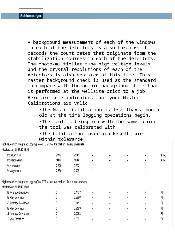
Master Calibrations.The Master Calibration for the PEx-TLD consists of determining a gain and offset for each window in each of the three detectors. This is done by comparing the four calibration measurements of the tool being calibrated to the response of the reference tool (that the processing model was based on) in the same conditions.

The Master Calibration results printed in the CSL consist of two parts. The first part is the Calibration Inversion Results which takes the calibrated count rates measured when the calibrated tool was in the aluminum block, passes those count rates through the inversion model, and compares the calculated density and Pef to the actual aluminum block density and Pef values. The process is also done for the magnesium block. The measured density values must fall within 10 kg/m3 and the measured Pef values must fall within 0.1 barns/e of the reference values.

The second part of the results is the Mean and Maximum Deviation List which lists the mean count rate deviation as a percentage and the maximum count rate deviation as a percentage during the four block measurements for all three detectors. Check the CSL for the calibration limits.

37

A background measurement of each of the windows in each of the detectors is also taken which records the count rates that originate from the stabilization sources in each of the detectors. The photo-multiplier tube high voltage levels and the crystal resolutions of each of the detectors is also measured at this time. This master background check is used as the standard to compare with the before background check that is performed at the wellsite prior to a job.

Here are some indicators that your Master Calibrations are valid:•The Master Calibration is less than a month old at the time logging operations begin.•The tool is being run with the same source the tool was calibrated with.•The Calibration Inversion Results are within tolerance.•The Mean and Maximum Deviations are within tolerance.•The background measurements fall within the nominal tolerance range.

Here is an example CSL from what could be a valid calibration.

38

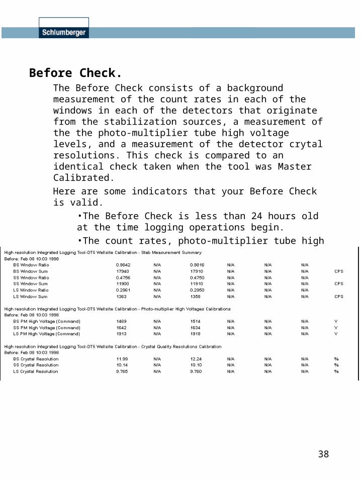
Before Check.The Before Check consists of a background measurement of the count rates in each of the windows in each of the detectors that originate from the stabilization sources, a measurement of the the photo-multiplier tube high voltage levels, and a measurement of the detector crytal resolutions. This check is compared to an identical check taken when the tool was Master Calibrated.

Here are some indicators that your Before Check is valid.•The Before Check is less than 24 hours old at the time logging operations begin.•The count rates, photo-multiplier tube high voltage levels, and the crystal resolutions fall within the tolerances set from the Master Calibration background measurement values. See the CSL for the individual tolerances.

Here is an example CSL from what could be a valid Before Check.

39

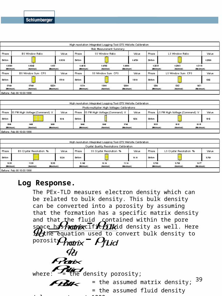
Log Response.The PEx-TLD measures electron density which can be related to bulk density. This bulk density can be converted into a porosity by assuming that the formation has a specific matrix density and that the fluid contained within the pore space has a specific fluid density as well. Here is the equation used to convert bulk density to porosity.

where: = the density porosity;

= the assumed matrix density;

= the assumed fluid density (always water at 1000 kg/m3); and,

= the measured bulk density.

d

matrix bulk

matrix fluid

d

bulkfluidmatrix

40

The bulk density outputs are RHOZ, RHO8, and RHOI while the density porosity outputs are DPHZ and DPH8.

The returning GR spectrum is also analyzed to provide a quantified value of the photo electric capture cross section of the formation. This Pef output is used to identify the formation lithology. The Pef outputs are PEFZ, PEF8, and PEFI.

The PEx-TLD also provides density standoff measurements, DSOZ, DSO8 and DSOI, which determine the distance between the pad face and the borehole wall through the forward model.

Meanwhile, the PEx-TLD offers the Density Correction curve (HDRA) which indicates the confidence the processing has in the density and porosity outputs. It is similar, but not the same, as the LDT’s DRHO.

The depth of investigation of the PEx-TLD is about 12 inches. Meanwhile, there are three vertical resolutions.

•DPHZ, RHOZ, PEFZ, and DSOZ have an 18” vertical resolution (these outputs provide the most accurate answers in poor borehole conditions - ie. washouts and rugose boreholes).•DPH8, RHO8, PEF8, and DSO8 have an 8” vertical resolution (these outputs are less robust to poor borehole conditions).•RHOI, PEFI, and DSOI have a 2” vertical resolution (please note that these 2” outputs are very susceptible to poor borehole conditions).

Here are some environmental factors that can affect your PEx-TLD log.•Gas in the pore space will cause the density porosity to read higher than true porosity by a factor of up to 1.5 due to the assumption that the formation fluid is water. •Oil in the pore space will cause the density porosity to read higher than true porosity by a factor of about 1.1 due to the assumption that the formation fluid is water.•Shale streaks within the formations will cause inaccuracies in the density porosity due to the matrix density assumption.

41

•Barite in the mud may cause inaccuracies in the formation Pef measurement due to its Pef value of 266 barns/e.•The PEx-TLD measurement is very sensitive to borehole rugosity due to the need for good pad contact. Therefore rugose boreholes will cause inaccuracies in your log. The smoother the borehole wall, the more accurate your log will be. In areas with oval holes, the short axis is usually but not always the smoothest axis and therefore is usually the axis to align the pad face in.•Heavy mud densities that approach the formation density will cause inaccuracies in your log because the forward model may not be able to distinguish the formation density from the mud density.

Here are some indicators that your PEx-TLD log is valid.•The PEx-TLD is within it’s operating range:

– 1400 kg/m3 < RHOZ < 3300 kg/m3;– 1.1 barns/e < PEFZ < 7.0 barns/e;– 0 < DSOZ < 40 mm; and,– the mud weight is less than 1500 kg/m3.

•The PEFZ, PEF8, and PEFI curves indicate a formation lithology that is consistent with the other log responses (ie. DT, RHOZ, NPOR, resistivity, GR, SP, etc.).•The logging speed is less than 3600 fph (18m/ min) for the curves with vertical resolutions of 18” and less than 1800 fph (9m/min) for the curves with vertical resolutions of 8” or 2”.•HDRA is positive, small, and has a baseline of 0 kg/m3. HDRA should read 0 kg/m3 in smooth boreholes with no mudcake. Values of 200 to 300 kg/m3 may be valid under some operating conditions.•HCAL is reading a smooth borehole.•DPHZ is positive if the correct matrix has been chosen and the porosity value falls within the expected range for that lithology.

42

•DPHZ should equal the PEx-CNL’s NPOR output in clean wet zones when the correct matrix has been chosen.•DPHZ should be about 1 p.u. more than NPOR in clean oil zones where the correct matrix has been chosen.•DPHZ should read much more than NPOR in clean gas zones where the correct matrix has been chosen.•In anhydrite, RHOZ reads 2980 kg/m3 and PEFZ reads 5 (see the chart for the matrix dependent DPHZ values).•In casing, RHOZ and DPHZ are invalid, PEFZ is greater than 10 barns/e, and HDRA is negative. •The PEFZ will flatline at 0.8 barns/e if low PEF formations like coal are encountered.


LQC Format.The HILTIndLQC and HILTLatLQC formats both contain three flags, four curves, and an analysis you can use to validate your log.

•The Density Detector flag (QCBSL) is triggered if the detector ADCs aren’t working, if the crystal scintillation time is too long, or if the detector high voltage loops become unstable.•The Density Computation flag (QCRH) is triggered if the formation density falls out of the forward model’s range, if a window in one of the detectors isn’t taken into account properly in the density processing, or if the computed SS density is greater than the LS density in formation densities greater than 2550 kg/m3.•The Pef Computation flag (QCPEF) is triggered if the formation Pef falls out of the forward model’s range, or if a window in one of the detectors isn’t taken into account properly in the Pef processing.•The Standard Resolution Density Standoff curve (DSOZ) should:

– agree with the PEx-MCFL’s RSOZ output;– read 0 mm in sections of smooth borehole with no

mudcake; and,– read less than 40 mm.

43

•The Density Correction curve (HDRA) was explained in the Log Response section. •The Pef Correction curve (HPRA) indicates the confidence the processing has in the Pef outputs. The higher the confidence, the closer HPRA is to 0. An HPRA value between -1 and 1 barns/e is normal.•HCAL can be used to explain standoff and the presence of mudcake, which both affect the PEx-TLD log.•The HRDD Processing FLAGS Statistical Analysis at the top of the format computes the percentage of the depth interval logged where the Density and Pef flags were triggered. If each one of the flags was individually triggered less than 10% of the time, the log is valid.

Repeatability.The PEx-TLD is a statistical measurement, and therefore its outputs do not have great repeatablity. Here are the repeatability limits.

•RHOZ, RHO8, and RHOI:– + 10 kg/m3 when DSOZ = 0 mm; and,– + 20 kg/m3 when DSOZ = 15 mm.

•DPHZ and DPH8 (these are translated from the density limit values):

– + 4 p.u. when DPHZ = 5 p.u. and DSOZ = 0 mm; – + 1 p.u. when DPHZ = 20 p.u. and DSOZ = 0 mm;– + 8 p.u. when DPHZ = 5 p.u. and DSOZ = 15 mm; and,– + 2 p.u. when DPHZ = 20 p.u. and DSOZ = 15 mm.

•PEFZ, PEF8, and PEFI:– + 0.15 barns/e when DSOZ = 0 mm; and,– + 0.2 barns/e when DSOZ = 15 mm.

44

PEx- Compensated Neutron Log

Applications.The PEx-CNL Log is used for:

•determining porosity;•identifying gas zones when run with a density or sonic log; and,•identifying formation lithology.

The PEx-CNL can be run in fluid filled open and cased holes, but not air filled holes.

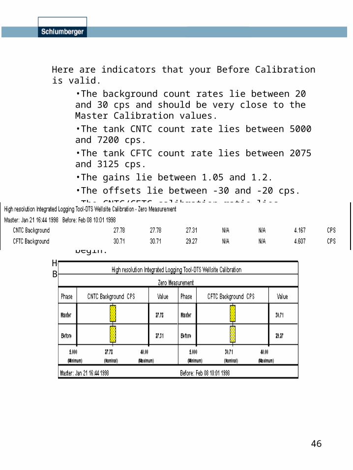
Master Calibrations.The Master Calibration consists of a two point calibration that sets a gain and offset for both the far and near detectors. The offsets should be negative and very close in magnitude to the background count rates that originate from the alpha sources near the far and near detectors.

Here are some indicators that you have a good Master Calibration.•The background count rates normally lie between 20 and 30 cps.•The tank CNTC count rate lies between 5000 and 7200 cps.•The tank CFTC count rate lies between 2075 and 3125 cps.•The gains lie between 1.05 and 1.2.•The offsets lie between -30 and -20 cps.•The CNTC/CFTC calibration ratio lies between 2.12 and 2.54.•The HGNS housing was measured and input into the calibration.•The tank temperature was measured and input into the calibration.•The Master Calibrations is less than 3 months old at the time logging operations begin.

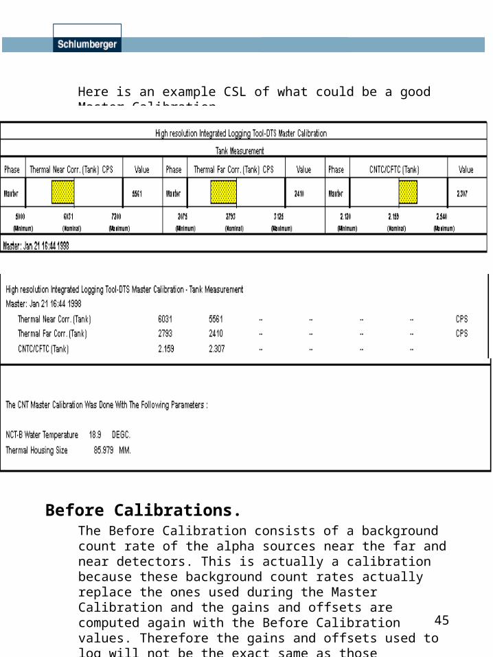
45

Here is an example CSL of what could be a good Master Calibration.

Before Calibrations.The Before Calibration consists of a background count rate of the alpha sources near the far and near detectors. This is actually a calibration because these background count rates actually replace the ones used during the Master Calibration and the gains and offsets are computed again with the Before Calibration values. Therefore the gains and offsets used to log will not be the exact same as those calculated when the Master Calibration was performed, though they will be very close.

The Before and Master Calibration background counts are also compared.

46

Here are indicators that your Before Calibration is valid.•The background count rates lie between 20 and 30 cps and should be very close to the Master Calibration values. •The tank CNTC count rate lies between 5000 and 7200 cps.•The tank CFTC count rate lies between 2075 and 3125 cps.•The gains lie between 1.05 and 1.2.•The offsets lie between -30 and -20 cps.•The CNTC/CFTC calibration ratio lies between 2.12 and 2.54.•The Before Calibrations are less than 24 hours old at the time logging operations begin.

Here is an example of what could be a valid Before Calibration.

47

Log Response.The PEx-CNL measures the hydrogen index of a formation. The hydrogen index is defined as follows.

HI = grams of H/cc of formation

grams of H/cc in H2O at 24C

where: HI= hydrogen index.

The PEx-CNL then converts this hydrogen index to a porosity by assuming that the pore space is filled with water, and not hydrocarbons. Most of the hydrogen in the formation is contained in the pore space as opposed to the matrix, therefore the neutron porosity output is very sensitive to the pore space fluid type. The second assumption is the matrix type you are logging in (sandstone, limestone, or dolomite).

The PEx-CNL offers porosity outputs with two vertical resolutions. NPOR has a 6” sampling rate while HNPO has a 2” sampling rate.

The porosity outputs are dependent on the matrix you choose.

Here is a list of environmental factors that affect the PEx-CNL porosity outputs.

•Large boreholes increase NPOR and HNPO due to the increased hydrogen and chlorine content in the borehole fluid. This is usually corrected for.•High temperatures cause NPOR and HNPO to read too low. This should be corrected for in borehole temperatures much above 25 C.•Standoff can cause NPOR and HNPO to read too high by up to 2 or 3 p.u. •Other environmental factors such as mudcake thickness, borehole salinity, mud weight, pressure, and formation salinity cause small porosity shifts that cancel each other out to within 1 or 2 p.u.•Gas in the pore spaces cause NPOR and HNPO to read much less than the true porosity due to the small hydrogen index of gas compared to water.

48

Oil in the pore spaces cause NPOR and HNPO to read slightly less than true porosity due to the slightly smaller hydrogen index of oil compared to water.

Here are some indicators that your PEx-CNL log is valid.•NPOR should equal the PEx-TLD’s DPHZ output in clean wet zones when the correct matrix has been chosen.•NPOR should be about 1 p.u. less than DPHZ in clean oil zones where the correct matrix has been chosen.•NPOR should read much less than DPHZ in clean gas zones where the correct matrix has been chosen.•NPOR should read -2 p.u. in an anhydrite when the chosen matrix is lime.•NPOR should read higher than true porosity in shales.•The logging speed is 3600 fph (18m/min) for NPOR and 1800 fph (9m/min) for HNPO.


LQC Formats.The HILTIndLQC and HILTLAtLQC both have one flag and one curve to help you validate your PEx-CNL log.

•The Neutron Porosity flag (QCPOR) is triggered if the difference between the environmentally corrected NPOR and the uncorrected NPOR is bigger than 10 p.u.•The Delta Neutron Porosity curve (DNPH) is the difference between the environmentally corrected NPOR and the uncorrected NPOR. DNPH should lie between -10 and 10 p.u.

Repeatability.The PEx-CNL is a statistical measurement, therefore it’s repeatability is not as good as other tools. It has the following repeatability values at the following porosities.

• + 1 p.u. from 0 to 20 p.u.•+ 2 p.u. at 30 p.u.•+ 6 p.u. above 45 p.u.

49

Borehole Compensated Sonic Log

Applications.The BHC Sonic Log is used for:

•correlating time based seismic profiles to depth;

•determining formation lithology;

•identifying fractures;

•identifying thin beds;

•determining formation porosity;

•determining secondary porosity when run with another porosity log; and,

•determining the presence of gas in the fomation pore space when run with a neutron porosity log.

The BHC Sonic must be run in fluid filled boreholes. The BHC Sonic must also be run in open hole to be used for the above formation evaluation applications.

Master Calibrations.There are no Master Calibrations for the SLCs, SDCs, or the DT operation of the DSLC. However, the DSLC cartridge has the ability to provide a high resolution delta t product, and to provide this accurate product, the sonde must be calibrated. The span of this measurement is 5”, therefore the measurement is much more sensitive to receiver spacing than the regular delta t measurement with a 2’ span. The calibration consists of establishing an upper transmitter delta t gain and a lower transmitter delta t gain. This sonde calibration occurs with the sonde in the sonic test tube or in unbonded casing. Here are how these gains are calculated.

50

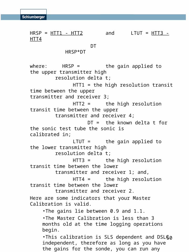
HRSP = HTT1 - HTT2 and LTUT = HTT3 - HTT4

DT HRSP*DT

where: HRSP = the gain applied to the upper transmitter high resolution delta t;

HTT1 = the high resolution transit time between the upper transmitter and receiver 3;

HTT2 = the high resolution transit time between the upper transmitter and receiver 4;

DT = the known delta t for the sonic test tube the sonic is calibrated in;

LTUT = the gain applied to the lower transmitter high resolution delta t;

HTT3 = the high resolution transit time between the lower transmitter and receiver 1; and,

HTT4 = the high resolution transit time between the lower transmitter and receiver 2.

Here are some indicators that your Master Calibration is valid.•The gains lie between 0.9 and 1.1.•The Master Calibration is less than 3 months old at the time logging operations begin.•This calibration is SLS dependent and DSLC independent, therefore as long as you have the gains for the sonde, you can run any DSLC you want with it.

Before Calibrations.There are no Before Calibrations or Checks for the BHC Sonic.

51

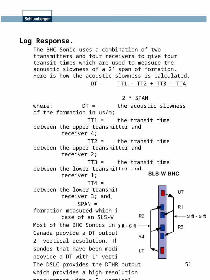
Log Response.The BHC Sonic uses a combination of two transmitters and four receivers to give four transit times which are used to measure the acoustic slowness of a 2’ span of formation. Here is how the acoustic slowness is calculated.

DT = TT1 - TT2 + TT3 - TT4

2 * SPAN

where: DT = the acoustic slowness of the formation in us/m;

TT1 = the transit time between the upper transmitter and receiver 4;

TT2 = the transit time between the upper transmitter and receiver 2;

TT3 = the transit time between the lower transmitter and receiver 1;

TT4 = the transit time between the lower transmitter and receiver 3; and,

SPAN = the interval of formation measured which is 2’ in the case of an SLS-W or -E in DT mode.

Most of the BHC Sonics in Western

Canada provide a DT output with a

2’ vertical resolution. There are some

sondes that have been modified which

provide a DT with 1’ vertical resolution.

The DSLC provides the DTHR output

which provides a high resolution

measurement with a 5” vertical

resolution. All of these measurements

have a depth of investigation of about

2” into the formation.

52

Here is a list of environmental factors that affect the BHC Sonic.•Gas in the borehole will cause cycle skipping.•Gas in formation will increase the DT value.•Fractures in the formation will cause DT spikes.•Washouts can increase the DT value (watch the caliper reading).•Uncompacted formations (like sandstone) can cause DT spiking.•Sonde eccentering will cause transit time stretch.•Formation reverberation can cause transit time noise.•Reverberation (continued ringing from the last transmitter firing) in carbonates can cause transit time noise.

Here are some indicators that your BHC Sonic log is valid.•DT reads the casing slowness in unbonded casing, usually 187 us/m or 192 us/m depending on the casing.•DT reads the matrix value or more with an increase in porosity.•DT will increase with an increase in formation shale content.•DT mirrors the GR response.•DT reads 164 us/m in anhydrite.•The logging speed is less than the software recommended logging speed.


LQC Format.The BHC Sonic format provides six curves to help you validate your BHC Sonic log.

•From the sonde diagram and the transit time definitions, you can see that TT1 and TT3 travel the same distance from transmitter to receiver. Therefore, TT1 and TT3 should have the same travel times and should overlay.•TT2 and TT4 also travel the same distance from transmitter to receiver. Therefore, TT2 and TT4 should also have the same travel times and should overlay.

53

•The caliper readings give a good indication of log quality because they indicate washouts and sometimes large fractures.•The DT curve was introduced and its expected responses were explained in the Log Response section.

Repeatability.The BHC Sonic takes an absolute reading and therefore is very accurate. The DT repeatability is + 7 us/m.

54

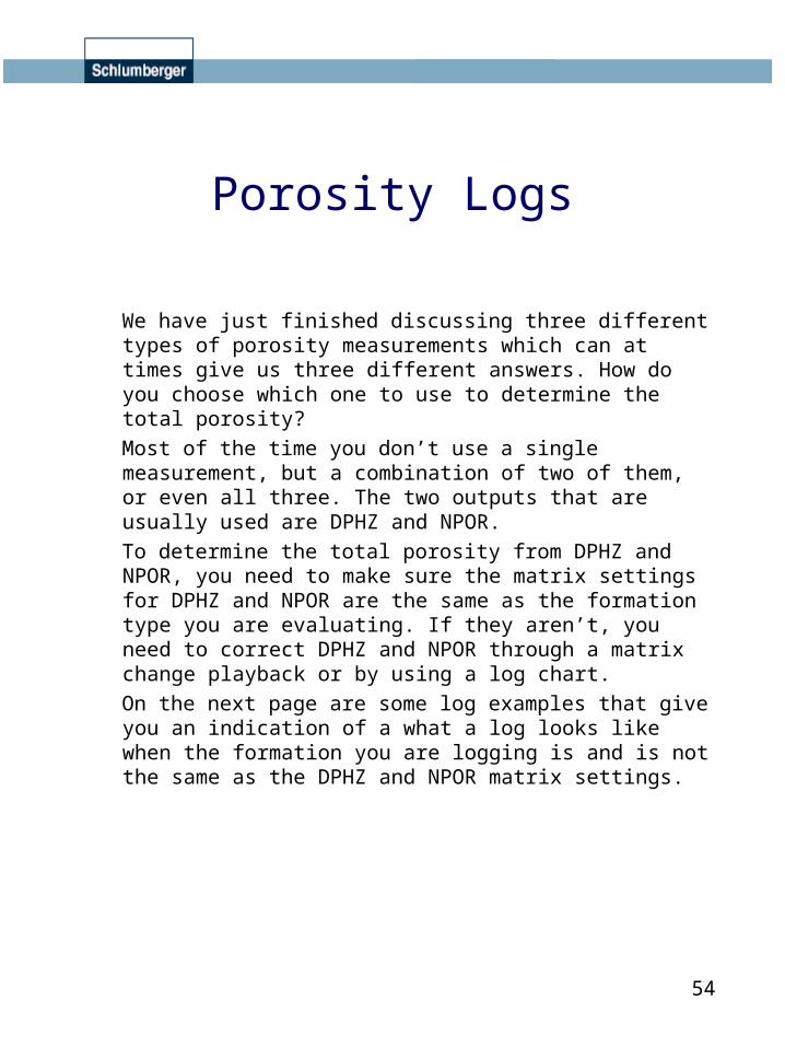
Porosity Logs

We have just finished discussing three different types of porosity measurements which can at times give us three different answers. How do you choose which one to use to determine the total porosity?

Most of the time you don’t use a single measurement, but a combination of two of them, or even all three. The two outputs that are usually used are DPHZ and NPOR.

To determine the total porosity from DPHZ and NPOR, you need to make sure the matrix settings for DPHZ and NPOR are the same as the formation type you are evaluating. If they aren’t, you need to correct DPHZ and NPOR through a matrix change playback or by using a log chart.

On the next page are some log examples that give you an indication of a what a log looks like when the formation you are logging is and is not the same as the DPHZ and NPOR matrix settings.

55

56

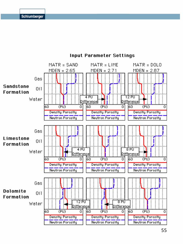
Now let’s consider some other conditions that can affect NPOR and DPHZ, such as gas in the pore space, oil in the pore space, washouts, shale formations, and salt formations. In this example, NPOR can replace NPHI and the matrix settings are limestone.

57

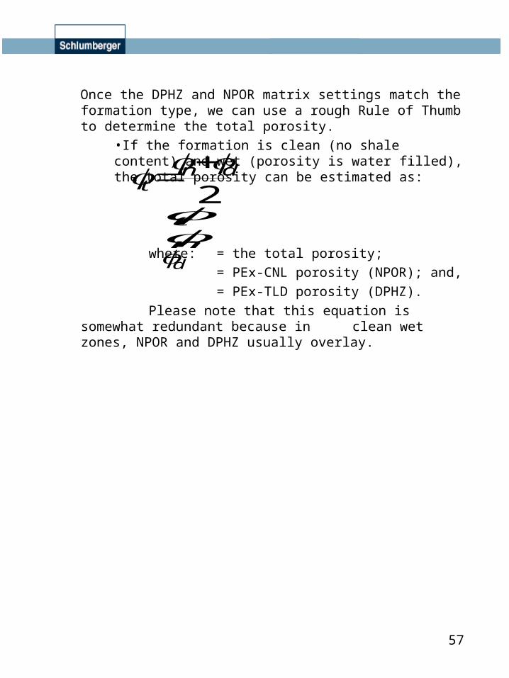
Once the DPHZ and NPOR matrix settings match the formation type, we can use a rough Rule of Thumb to determine the total porosity.

•If the formation is clean (no shale content) and wet (porosity is water filled), the total porosity can be estimated as:

where: = the total porosity;

= PEx-CNL porosity (NPOR); and,

= PEx-TLD porosity (DPHZ).

Please note that this equation is somewhat redundant because in clean wet zones, NPOR and DPHZ usually overlay.

t

n d2

d

nt

58

Calipers

We currently run a plethora of calipers in Western Canada. This section will provide the general techniques you can use to validate your caliper logs.

Applications.Calipers are used for:

•measuring the hole diameter;

•calculating cement and hole volumes;

•indicating log quality; and;

•providing a borehole size input for borehole correstions.

Calipers can be run in all borehole mud types including air filled holes.

Master Calibrations.There are no Master Calibrations for any of the mechanical caliper devices we use in Western Canada.

Before Calibrations.There are Before Calibrations for the calipers we use in Western Canada which consist of a two point calibration which determines a gain and offset for each caliper measurement.

Here are some general indicators that your Before Calibrations are valid.

•The Before Calibration was performed within 24 hours of beginning the logging operations.

•The gains lie between 0.9 and 1.1 (except for the EDAC whose gains are approximately 2 and 5 for CAL1 and CAL2 respectively).

•The offsets are close to 0 (except fot the EDAC whose offsets can be negative or positive and large or small).

59

Log Response.In casing, calipers should read the internal diameter of the casing.

In the foothills of Western Canada, breakout usually occurs to our boreholes. Breakout is an elongation of one of the axes of the borehole due to tectonic stresses in the area (mountains are another result of the same tectonic stresses). These tectonic stresses cause oval holes which have a minor axis whose diameter can be close to bit size and a major axis whose diameter can be much larger than bit size. Most of the time the minor axis is smoother, therefore providing a better axis to log our pad devices and contact tools (ie. PEx-CNL and PEx-TLD). The dual axis caliper is often used to measure both axes so we calculate more accurate hole and cement volumes, and so we can ensure we are logging the smoother axis to gain better data with our pad devices and contact tools.

The integrated hole and cement volumes presented in the summary at the top of the format should make sense.


LQC Format.The HILTIndLQC and HILTLatLQC formats both display the PEx-Caliper HCAL whose log response has been explained in the Log Response section.

Repeatability.Calipers usually offer good repeatability as long as they are logging the same axis during both passes and the borehole conditions haven’t changed (ie. sloughing).

•The repeatability of the PEx-Caliper is + 6 mm.

60

Offset Logs

The most valuable tool a geologist has in evaluating the validity of a log is his or her knowledge of the log responses in that area. Since most geologists work very few fields at a time, they become experts in interpreting log responses in those fields. They can spot a valid log without even having to look at an offset because they have memorized the log responses.

As a Field Engineer, you will be exposed to many more fields, but with less exposure in any one field. Therefore, your expertise in any one field may not be enough to validate your logs.

Offsets help you:

•correlate formation tops (sandstones, anhydrites, coal streaks, etc);

•compare resistivities, porosities, delta ts, grs, sp deflections, and more;

•confirm calibrations; and,

•identify the validity of anomalous repsonses.

These are only a few of the valuable uses offset logs provide.

They are especially handy when you’re in a field you’ve never logged before, or if your log response doesn’t look typical.

Offset logs are usually available in district libraries. If not, and you have time, try to obtain them from the sales engineer.

When you arrive on location, talk to the geologist. He or she will probably have a set of offset logs. Equally as important, he or she will be able to tell you the primary and secondary zones of interest, formation tops, formation markers, expected porosities, expected unusual responses. The wellsite geologist is a useful resource.

61

Repeatability

Repeatability is an important but sometimes little understood technique in validating logs.

A log that repeats indicates that the tool you are running is responding the same way to the same conditions. It does not necessarily indicate that the response is valid (ie. due to bad calibrations, a wrong GSR-J source, etc.)

The standard repeat section is usually logged over the bottom 60 m of the well because that is where the primary zone of interest is. However, depending on factors such as hole conditions, you may want to pull the repeat uphole somewhere.

The emphasis is moving away from repeat sections and towards LQC formats to validate logs. However, the repeat section remains a valuable tool used to confirm anomalous log responses that may otherwise be blamed on a hardware failure.

62

Depth

It is imperative that the logs we present are on depth with each other. This means that:

•the toolstring measure points are correct;

•curves presented within a single format must be on depth with each other (ie. GR on depth with NPOR);

•curves presented on different formats must be on depth with each other (ie. NPOR on depth with AHT30); and,

•curves from different descents must be on depth with each other (ie. SP on depth with DT).

The wrong completion decision has been made on several wells because the curves were not on depth with each other. It’s a simple and essential step in the validation process.

63

Presentation

This is the last topic covered in this package, but it is not the least important. The presentation of the information you provide the client is an important factor in the way the client will base his or her decisions on that well and possibly other wells in the area.

Most of the time your products are delivered straight to the client. You are the last Quality Control Check Point. Therefore it is imperativethat you make sure you deliver a quality product. This means spending as much effort on presentation and delivery as you do on acquisition.

Clients have made the wrong completion decision on wells because of improper scales (ie. DPHZ and NPOR scales), improper coding (ie. AIT invasion curve codings), etc.

When validating your logs, check:

•the header information (ie. UWI);

•the scales;

•the coding;

•the labels; and,

•the first readings.

These are just a few example presentation particulars you need to watch for.

64

Further References

This package is intended to give you an overview of the techniques you should use on every job to validate your PLATFORM EXPRESS - BHC Sonic Logs. If you would like more information on any of these subjects, while in the shop or on a job, I recommend talking to any and all of the Sales Engineers and members of the Product Development Team.

If you want to read up on any of these topics, try:

•Basic Open Hole Log Interpretation (ie. Open Hole Basics);

•The HILT-B Field Engineeer’s Manual;

•Log Interpretation Charts;

•Log Quality Control Manual on CD-Rom; and, of course,

•the Web.

65

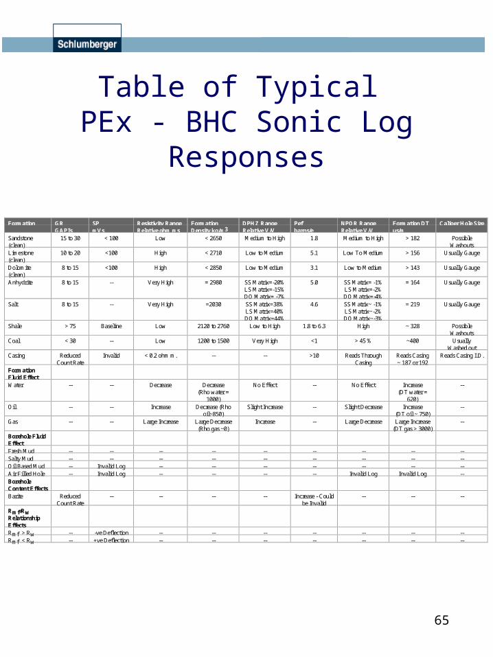
Table of Typical PEx - BHC Sonic Log

Responses

Formation GRGAPIs

SPmVs

Resistivity RangeRelative ohm ms

FormationDensity kg/m3

DPHZ RangeRelative V/V

Pefbarns/e

NPOR RangeRelative V/V

Formation DTus/m

Caliper Hole Size

Sandstone(clean)

15 to 30 < 100 Low < 2650 Medium to High 1.8 Medium to High > 182 PossibleWashouts

Limestone(clean)

10 to 20 <100 High < 2710 Low to Medium 5.1 Low To Medium > 156 Usually Gauge

Dolomite(clean)

8 to 15 <100 High < 2850 Low to Medium 3.1 Low to Medium > 143 Usually Gauge

Anhydrite 8 to 15 -- Very High = 2980 SS Matrix=-20%LS Matrix=-15%DO Matrix= -7%

5.0 SS Matrix= -1%LS Matrix=-2%DO Matrix=-4%

= 164 Usually Gauge

Salt 8 to 15 -- Very High =2030 SS Matrix=38%LS Matrix=40%DO Matrix=44%

4.6 SS Matrix~ -1%LS Matrix~-2%DO Matrix~-3%

= 219 Usually Gauge

Shale > 75 Baseline Low 2120 to 2760 Low to High 1.8 to 6.3 High ~ 328 PossibleWashouts

Coal < 30 -- Low 1200 to 1500 Very High <1 > 45 % ~400 UsuallyWashed out

Casing ReducedCount Rate

Invalid < 0.2 ohm m. -- -- >10 Reads ThroughCasing

Reads Casing~ 187 or 192

Reads Casing I.D.

FormationFluid EffectWater -- -- Decrease Decrease

(Rho water =1000)

No Effect -- No Effect Increase(DT water =

620)

--

Oil -- -- Increase Decrease (Rhooil~850)

Slight Increase -- Slight Decrease Increase(DT oil ~ 750)

--

Gas -- -- Large Increase Large Decrease(Rho gas ~0)

Increase -- Large Decrease Large Increase(DT gas > 3000)

--

Borehole FluidEffectFresh Mud -- -- -- -- -- -- -- -- --Salty Mud -- -- -- -- -- -- -- -- --Oil Based Mud -- Invalid Log -- -- -- -- -- -- --Air Filled Hole -- Invalid Log -- -- -- -- Invalid Log Invalid Log --BoreholeContent EffectsBarite Reduced

Count Rate-- -- -- -- Increase - Could

be Invalid-- -- --

Rmf/RwRelationshipEffectsRmf > Rw -- -ve Deflection -- -- -- -- -- -- --Rmf < Rw -- +ve Deflection -- -- -- -- -- -- --