

MEscopeVES™
VES-4000 Modal Analysis
(May 13, 2020)

Notice
Information in this document is subject to change without notice and does not represent a commitment on the part of
Vibrant Technology. Except as otherwise noted, names, companies, and data used in examples, sample outputs, or
screen shots, are fictitious and are used solely to illustrate potential applications of the software.
Warranty
Vibrant Technology, Inc. warrants that (a) the software in this product will perform substantially in accordance with
the accompanying documentation, for a period of one (1) year from the date of delivery, and that (b) any hardware
accompanying the software will be free from defects in materials and workmanship for a period of one (1) year from
the date of delivery. During this period, if a defect is reported to Vibrant Technology, replacement software or
hardware will be provided to the customer at no cost, excluding delivery charges. Any replacement software will be
warranted for the remainder of the original warranty period or thirty (30) days, whichever is longer.
This warranty shall not apply to defects resulting from improper or inadequate maintenance by the customer, customer
supplied software or interfacing, unauthorized modification or misuse, operation outside of the environmental
specifications for the product, or improper site preparation or maintenance.
If the software does not materially operate as warranted above, the sole remedy of the customer (and the entire
liability of Vibrant Technology) shall be the correction or detour of programming errors attributable to Vibrant
Technology. The software should not be relied on as the sole basis to solve a problem whose incorrect solution could
result in injury to a person or property. If the software is employed in such a manner, it is at the entire risk of the
customer, and Vibrant Technology disclaims all liability for such misuse.
NO OTHER WARRANTY IS EXPRESSED OR IMPLIED. VIBRANT TECHNOLOGY SPECIFICALLY MAKES
NO WARRANTY OF ANY KIND WITH REGARD TO THIS MATERIAL, INCLUDING, BUT NOT LIMITED
TO, THE IMPLIED WARRANTIES OF MERCHANT ABILITY AND FITNESS FOR A PARTICULAR
PURPOSE.
THE REMEDIES PROVIDED HEREIN ARE THE CUSTOMER'S SOLE AND EXCLUSIVE REMEDIES.
VIBRANT TECHNOLOGY SHALL NOT BE LIABLE FOR ANY DIRECT, INDIRECT, SPECIAL,
INCIDENTAL, OR CONSEQUENTIAL DAMAGES IN CONNECTION WITH THE FURNISHING,
PERFORMANCE, OR USE OF THIS PRODUCT, WHETHER BASED ON CONTRACT, TORT, OR ANY
OTHER LEGAL THEORY.
The software described in this document is copyrighted by Vibrant Technology, Inc. or its suppliers and is protected
by United States copyright laws and international treaty provisions. Unauthorized reproduction or distribution of this
program, or any portion of it, may result in severe civil and criminal penalties, and will be prosecuted to the maximum
extent possible under the law.
You may make copies of the software only for backup or archival purposes. No part of this manual may be
reproduced or transmitted in any form or by any means for any purpose without the express written permission of
Vibrant Technology.
Copyright © 1992-2020 by Vibrant Technology, Inc. All rights reserved. Printed in the United States of America.
Vibrant Technology, Inc.
12835 E. Arapahoe Rd.
Tower II, Suite 600
Centennial, CO 80112 USA
phone: (831) 430-9045
fax: (831) 430-9057
E-mail: [email protected]
http://www.vibetech.com

3
Table of Contents
VES-4000 Modal Analysis............................................................................................................................. 8
Additional Data Block (BLK) Commands ................................................................................................................ 8
Additional Shape Table (SHP) Commands ............................................................................................................... 8
Data Block (BLK) Transform Menu ............................................................................................................... 9
Transform | Increase Resolution ................................................................................................................................ 9
Transform | Window M#s | (DeConvolution window) .............................................................................................. 9
What is a Modal Model? .............................................................................................................................. 10
Single Reference Modal Test ...................................................................................................................... 10
Roving Impact Test ................................................................................................................................................. 10
Roving Response Test ............................................................................................................................................. 10
Maxwell's Reciprocity ............................................................................................................................................. 10
What is FRF-Based Curve Fitting? .......................................................................................................................... 11
Three Curve Fitting Steps ........................................................................................................................................ 11
FRFs in Terms of Modal Parameters .......................................................................................................... 11
Partial Fraction Expansion of the FRF Matrix ......................................................................................................... 11
Global versus Local Curve Fitting ........................................................................................................................... 12
Modal Residues ....................................................................................................................................................... 12
FRF-based Curve Fitting ......................................................................................................................................... 12
Frequency & Damping Estimates ............................................................................................................... 12
Damped Natural Frequency ..................................................................................................................................... 12
Modal Damping ....................................................................................................................................................... 12
Percent of Critical Damping .................................................................................................................................... 12
Damping Decay Constant ........................................................................................................................................ 12
Half Power Point (3 dB bandwidth) Damping ......................................................................................................... 13
Quality Factor and Loss Factor ................................................................................................................................ 13
S-Plane Plot of Frequency & Damping ................................................................................................................... 13
Residues Versus Mode Shapes .................................................................................................................. 15
Relationship Between Residues & Mode Shapes .................................................................................................... 15
Mode Shape Scaling ................................................................................................................................................ 15
Fundamental Modal Testing Criterion ..................................................................................................................... 15
Mode Shape Node Points......................................................................................................................................... 15
Local Versus Global Modes .................................................................................................................................... 16
Curve Fitting Guidelines .............................................................................................................................. 16
1. Overlay the FRFs ................................................................................................................................................. 16
2. Inspect the Impulse Response Functions (IRFs) .................................................................................................. 16

VES-4000 Modal Analysis
4
3. Use the Mode Indicator to Count Peaks .............................................................................................................. 16
4. Use Quick Fit First .............................................................................................................................................. 17
5. Use the Band cursor & Quick Fit ......................................................................................................................... 17
6. Verify Fundamental Mode Shapes with the Animated Display ........................................................................... 17
7. Compare Results from Different Curve Fitting Methods .................................................................................... 18
Curve Fit | Open Curve Fitting .................................................................................................................... 18
Vertical Splitter Bars ............................................................................................................................................... 19
Horizontal Splitter Bars ........................................................................................................................................... 19
Modal Parameters Spreadsheet ................................................................................................................................ 19
Select Mode Column ........................................................................................................................................... 19
Frequency & Damping Columns ......................................................................................................................... 19
Residue Magnitude & Phase Columns ................................................................................................................ 20
Methods Columns ................................................................................................................................................ 20
Showing & Hiding Spreadsheet Columns ........................................................................................................... 20
Default Spreadsheet Column Widths ................................................................................................................... 20
Spreadsheet Text Cells ........................................................................................................................................ 20
Mode Indicator Tab ..................................................................................................................................... 21
Frequency & Damping Curve Fitting Methods ............................................................................................ 22
Polynomial Method ................................................................................................................................................. 22
Global Curve Fitting ................................................................................................................................................ 22
Non-Stationary Data ................................................................................................................................................ 22
Global Versus Local Curve Fitting .......................................................................................................................... 22
Frequency Damping Tab ............................................................................................................................. 22
Global Polynomial Method ...................................................................................................................................... 22
Local Polynomial Method ....................................................................................................................................... 22
Vertical Frequency Lines ......................................................................................................................................... 23
Horizontal Damping Lines ...................................................................................................................................... 23
Extra Numerator Polynomial Terms ........................................................................................................................ 24
Residue Curve Fitting Methods ................................................................................................................... 24
Lightly-Coupled Modes ........................................................................................................................................... 24
Peak Method ............................................................................................................................................................ 24
Closely Coupled Modes ........................................................................................................................................... 25
Polynomial Method ................................................................................................................................................. 25
Extra Numerator Polynomial Terms ........................................................................................................................ 25
Residues Save Shapes Tab........................................................................................................................ 25
Fit Function ............................................................................................................................................................. 25
Save Shapes Button ................................................................................................................................................. 26

5
Exponential Window Damping Removal ................................................................................................................ 26
Residue mode shapes ............................................................................................................................................... 26
Curve Fitting OMA Measurements .............................................................................................................. 27
Output-only Measurements ..................................................................................................................................... 27
Flat Force Spectrum ................................................................................................................................................. 27
Curve Fitting Fourier Spectra .................................................................................................................................. 27
Curve Fitting Cross Spectra ..................................................................................................................................... 27
Curve Fitting ODS FRFs ......................................................................................................................................... 27
Data Block (BLK) Curve Fit Menu ............................................................................................................... 28
Curve Fit | Quick Fit ................................................................................................................................................ 28
Quick Fit Steps .................................................................................................................................................... 28
Improving Quick Fit Results ............................................................................................................................... 28
Count Peaks Un-Checked ........................................................................................................................................ 29
Curve Fit | Delete All Fit Data ................................................................................................................................. 29
Curve Fit | Mode Indicator | Count Peaks ................................................................................................................ 29
Curve Fit | Mode Indicator | Clear Indicator ............................................................................................................ 29
Curve Fit | Mode Indicator | Smooth Indicator ........................................................................................................ 29
Curve Fit | Mode Indicator | CMIFs ........................................................................................................................ 30
Curve Fit | Mode Indicator | MMIFs ........................................................................................................................ 30
Curve Fit | Mode Indicator | Copy CMIFs ............................................................................................................... 30
Curve Fit | Mode Indicator | Copy MMIFs .............................................................................................................. 30
Curve Fit | Frequency Damping | Number of Modes ............................................................................................... 30
Curve Fit | Frequency Damping | Frequency Damping ........................................................................................... 30
Curve Fit | Residues ................................................................................................................................................. 30
Curve Fit | Modal Parameters | Sort by Frequency .................................................................................................. 30
Curve Fit | Modal Parameters | Select All Modes, Select None, Invert Selection ................................................... 30
Curve Fit | Modal Parameters | Delete Modes ......................................................................................................... 30
Curve Fit | Modal Parameters | Save Shapes ........................................................................................................... 30
Curve Fit | Modal Parameters | MAC ...................................................................................................................... 30
Curve Fit | Fit Functions | Clear Fit Functions ......................................................................................................... 30
Curve Fit | Fit Functions | Synthesize Fit Functions ................................................................................................ 31
Curve Fit | Fit Functions | Fit Functions .................................................................................................................. 31
Curve Fit | Fit Functions | Copy Fit Functions ......................................................................................................... 31
Curve Fit | Close Curve Fitting ................................................................................................................................ 31
Shape Table (SHP) Display Menu .............................................................................................................. 32
Display | MAC ......................................................................................................................................................... 32
What is MAC? ......................................................................................................................................................... 32

VES-4000 Modal Analysis
6
What is CoMAC? .................................................................................................................................................... 33
MAC Window Commands ...................................................................................................................................... 33
File | Copy Graphics to Clipboard ....................................................................................................................... 33
File | Print ............................................................................................................................................................ 33
File | Close ........................................................................................................................................................... 33
Display | Spreadsheet ........................................................................................................................................... 33
Display | 3D Bar Chart ........................................................................................................................................ 33
Display | Values ................................................................................................................................................... 33
Display | MAC, CoMAC ..................................................................................................................................... 33
Structure Options Animation Tab ........................................................................................................................ 34
Display | SDI ........................................................................................................................................................... 34
What is SDI? ............................................................................................................................................................ 34
SDI Window Commands ......................................................................................................................................... 35
File | Copy Graphics to Clipboard ....................................................................................................................... 35
File | Print ............................................................................................................................................................ 35
File | Close ........................................................................................................................................................... 35
Display | Spreadsheet ........................................................................................................................................... 35
Display | 3D Bar Chart ........................................................................................................................................ 35
Display | Values ................................................................................................................................................... 35
Structure Options Animation Tab ........................................................................................................................ 36
Display | Participation .............................................................................................................................................. 36
What Is Shape Participation? ................................................................................................................................... 36
Participation Window Commands ........................................................................................................................... 36
File | Copy Graphics to Clipboard ....................................................................................................................... 36
File | Print ............................................................................................................................................................ 36
File | Close ........................................................................................................................................................... 36
Display | Spreadsheet ........................................................................................................................................... 37
Display | 3D Bar Chart ........................................................................................................................................ 37
Display | Value .................................................................................................................................................... 37
Display | Real Part, Imaginary Part, Magnitude .................................................................................................. 37
Shape Table (SHP) Tools Menu ................................................................................................................. 37
Tools | Synthesize FRFs .......................................................................................................................................... 37
Residue mode shapes ........................................................................................................................................... 37
UMM mode shapes .............................................................................................................................................. 37
What is a Modal Model?.......................................................................................................................................... 38
Overlaying Synthesized & Measured FRFs ............................................................................................................. 38
Tools | Scaling | UMM to Residue Shapes .............................................................................................................. 39

7
Tools | Scaling | Residues to UMM Shapes ............................................................................................................. 39
Tools | Scaling | Un-Scaled to Scaled Shapes .......................................................................................................... 40
Tools | Scaling | Rapid Test Residues to UMM Shapes ........................................................................................... 40
What is a Rapid Test? .............................................................................................................................................. 40

VES-4000 Modal Analysis
8
VES-4000 Modal Analysis
If the VES-4000 Modal Analysis option is authorized by your MEscope license, the following commands are
enabled in the Data Block (BLK) and Shape Table (SHP) windows. Check Help | About to verify authorization
of this option.
Additional Data Block (BLK) Commands
• Transform | Increase Resolution
• Transform | Window M#s (DeConvolution window)
• Curve Fit | Open Curve Fitting
• Curve Fit | Delete All Fit Data
• Curve Fit | Quick Fit
• Curve Fit | Mode Indicator Menu
• Curve Fit | Frequency Damping Menu
• Curve Fit | Residues
• Curve Fit | Modal Parameters Menu
• Curve Fit | Fit Functions Menu
• Curve Fit | Close Curve Fitting
Additional Shape Table (SHP) Commands
• Display | MAC
• Display | SDI
• Display | Participation
• Tools | Synthesize FRFs
• Tools | Scaling | UMM to Residue Shapes
• Tools | Scaling | Residue to UMM Shapes
• Tools | Scaling | Unscaled to Scaled Shapes
• Tools | Scaling | Rapid Test Residues to UMM Shapes

9
Data Block (BLK) Transform Menu
Transform | Increase Resolution
Increases the resolution (reduces the spacing) between samples of data in either time or frequency domain data.
• FRF-based curve fitting is improved by increasing the number of samples surrounding each resonance peak
• Linear interpolation is used between adjacent samples to create new samples evenly spaced between the
original samples
• Each time this command is executed, the number of samples (Block Size) is doubled in a Data Block (BLK).
Transform | Window M#s | (DeConvolution window)
Applies the DeConvolution window to all (or selected) M#s in a Data Block (BLK).
• The DeConvolution window must be applied to output-only measurements before FRF-based curve fitting
methods can be used on them
The DeConvolution window smoothly zeroes (removes) the second half of each time waveform
• When this command is executed, the following steps are carried out,
All M#s are transformed to the time domain
The DeConvolution window is applied to all (or selected) M#s
All M#s are transformed back to the frequency domain
• The figures below show Cross spectra before & after the DeConvolution window was applied to them
Notice that noise is also removed from the measurements by the DeConvolution window
Cross Spectra Before Devolution Windowing.
Cross Spectra After Devolution Windowing.
What is a Modal Model?
10
What is a Modal Model?
A Modal Model is a set of mode shapes that has been scaled to preserve the mass, stiffness & damping properties
of a structure.
• MEscope uses two different Modal Models, Residue mode shapes and UMM mode shapes
• Residue mode shapes are obtained by curve fitting a set of calibrated FRFs
Residue mode shapes can also be obtained by re-scaling UMM mode shapes
see Tools | Scaling | UMM to Residue Shapes
• UMM mode shapes are obtained by re-scaling Residue mode shapes
see Tools | Scaling | Residues to UMM Shapes
• UMM mode shapes are also obtained by solving for the modes of an FEA model
Single Reference Modal Test
The most common type of Experimental Modal Analysis (EMA) is done using a single reference.
• A single reference EMA can be performed in two ways
Using a fixed reference response sensor and a roving exciter
Using a fixed reference exciter and a roving response sensor
Roving Impact Test
In a roving impact test, a single fixed reference response sensor is used, and the structure is excited at multiple
DOFs using a roving impactor.
• Each FRF is calculated between the response signal from the fixed DOF and the excitation signal from a
different DOF
• The impact hammer applies a broad-band impulsive force to the structure, which excites many resonances at
a time
• The excitation force is measured with a load cell attached to the head of the hammer
Roving Response Test
In a roving response test, a single fixed reference exciter is used to excite the structure, and a roving response
sensor is used to measure responses at multiple DOFs.
• Each FRF is calculated between the excitation signal and the response signal from a different DOF
• A reference excitation force can be provided in two ways,
Attach a shaker to the structure and drive it with a broad band signal
Impact the structure at the same DOF throughout the modal test
Maxwell's Reciprocity
Maxwell’s Reciprocity: The structural response at DOF A due to an excitation force applied at DOF B is the
same as the structural response at DOF B due to the same excitation force applied at DOF A.
• Maxwell’s Reciprocity is assumed to be valid in a single-reference modal test
Any Reference DOF can be used during a single-reference modal test
A Roving Impact test provides mode shapes with a shape component for each DOF where the structure is
impacted
A Roving Response test provides mode shapes with a shape component for each DOF of the response
sensor
11
Using a tri-axial response sensor in a Roving Response test, provides mode shapes that contain 3D
motion of the structure at each response point
What is FRF-Based Curve Fitting?
FRF-based curve fitting is a process of matching an FRF parametric model in a least-squared-error sense to a set
of experimental data. It is also referred to as modal parameter estimation.
• FRF-based curve fitting provides modal parameters (frequency, damping & mode shape) for each mode
that is identified in the frequency span of the experimental data
• After curve fitting is completed, mode shapes are stored into a Shape Table (SHP) from which they can be
displayed in animation on a 3D model of the test article
Three Curve Fitting Steps
In MEscope, curve fitting is done in three steps.
• Determine the Number of Modes in a frequency band of experimental data
• Estimate modal Frequency & Damping for all modes in the frequency band
• Estimate modal Residues (mode shape components) for each mode and each measurement function
FRFs in Terms of Modal Parameters
FRF-based curve fitting assumes that any FRF calculated between two DOFs of a vibrating structure can be
completely represented in terms of modal parameters.
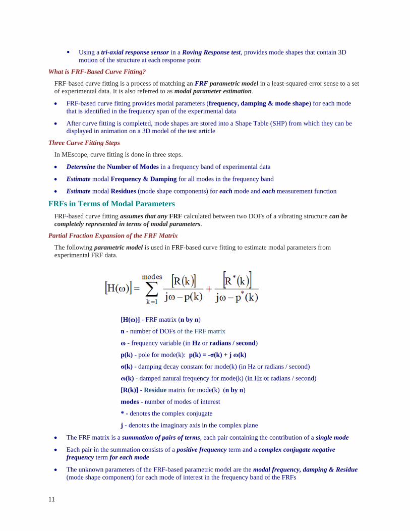
Partial Fraction Expansion of the FRF Matrix
The following parametric model is used in FRF-based curve fitting to estimate modal parameters from
experimental FRF data.
[H(ɷ)] - FRF matrix (n by n)
n - number of DOFs of the FRF matrix
ɷ - frequency variable (in Hz or radians / second)
p(k) - pole for mode(k): p(k) = -σ(k) + j ɷ(k)
σ(k) - damping decay constant for mode(k) (in Hz or radians / second)
ɷ(k) - damped natural frequency for mode(k) (in Hz or radians / second)
[R(k)] - Residue matrix for mode(k) (n by n)
modes - number of modes of interest
* - denotes the complex conjugate
j - denotes the imaginary axis in the complex plane
• The FRF matrix is a summation of pairs of terms, each pair containing the contribution of a single mode
• Each pair in the summation consists of a positive frequency term and a complex conjugate negative
frequency term for each mode
• The unknown parameters of the FRF-based parametric model are the modal frequency, damping & Residue
(mode shape component) for each mode of interest in the frequency band of the FRFs
Frequency & Damping Estimates
12
• The residues obtained from curve fitting one or more FRFs are saved as a Residue mode shape for each
mode
Global versus Local Curve Fitting
During global curve fitting, a global frequency & damping estimate is obtained from all FRFs for each mode.
During local curve fitting, a local frequency & damping estimate is obtained from each FRF for each mode.
• The denominator of each term in the FRF parametric model contains the same pole (frequency & damping)
for each mode
Modal frequency & damping are global properties of a structure
Modal Residues
A Residue is the "strength" of a resonance.
• The larger its Residue value, the stronger a resonance is relative to other resonances
Residue units = (FRF units) x (radians / second)
• Each Residue has the same DOFs as the FRF from which is was obtained by FRF-based curve fitting
FRF-based Curve Fitting
During FRF-based curve fitting, four modal parameters are estimated for each mode
• The pole location or frequency & damping of each mode
p(k) = -σ (k) + j ɷ (k), p(k) - pole of mode(k)
• The complex Residue (magnitude & phase) for each mode
Frequency & Damping Estimates
Damped Natural Frequency
The frequency estimate for each mode(k) is listed as the damped natural frequency ɷ (k) in the Modal
Parameters spreadsheet.
Modal Damping
The damping estimate for each mode(k) is listed as the damping decay constant and the percent of critical
damping in the Modal Parameters spreadsheet
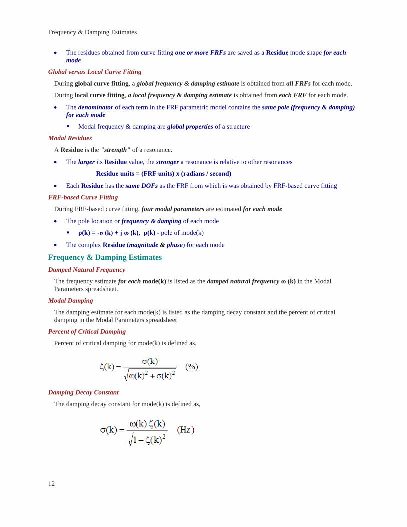
Percent of Critical Damping
Percent of critical damping for mode(k) is defined as,
Damping Decay Constant
The damping decay constant for mode(k) is defined as,

13
Half Power Point (3 dB bandwidth) Damping
The damping decay constant is one-half of the width of the resonance peak.
• The half power points are 3 dB less than the power at the resonance peak
• This half power point bandwidth estimate of modal damping is also called the 3 dB bandwidth damping
• The width of the resonance peak in an FRF at 70.7% of the magnitude of the resonance peak is equal to twice
the damping decay constant
The wider the resonance peak, the greater the modal damping
Quality Factor and Loss Factor
The Loss factor is equal to twice the percent of critical damping
• The Quality Factor Q(k) is the inverse of the Loss factor
S-Plane Plot of Frequency & Damping
The four definitions of modal frequency & damping are plotted on the top view of the S-plane (or complex
frequency plane) below.
S-plane Showing Modal Frequency & Damping Terms.

14
• Modal frequency & damping are defined in several ways,
p(k) = - σ (k) + j ɷ (k) pole location of mode(k) (Hz)
ɷ (k) damped natural frequency of mode(k) (Hz)
σ k) damping decay constant (also called 3 dB bandwidth or half power point damping) of
mode(k) (Hz)
ς(k) damping ratio (%)
Ω(k) undamped natural frequency of mode(k) (Hz)
Half Power Point
Bandwidth
(3 dB Bandwidth)
Damping Ratio
(Percent of Critical)
Decay Constant
Loss Factor
Quality Factor

15
Residues Versus Mode Shapes
The FRF matrix can be expressed in terms of modal poles & mode shapes as
p(k) pole of mode(k) (Hz)
p(k) = - σ (k) + j ɷ (k)
A(k) scaling constant for mode (k)
u(k) mode shape for the mode (k) (n - vector)
t denotes the transposed vector
Relationship Between Residues & Mode Shapes
The Residue matrix [R(k)] for mode(k) is written in terms its mode shape vector u(k) as
• Each mode shape (a column vector u(k), is multiplied by itself transposed (a row vector u(k)t)
• This vector product, (a column vector times a row vector), is called an outer product, and it yields a matrix
• Residue matrix [R(k)] Outer product of mode shape vectors multiplied by the scaling constant A(k)
The Residue matrix has unique engineering units
A mode shape is unique in shape but has no engineering units
The scaling constant A(k) is required to make the Residue matrix equal to the outer product of mode
shape vectors
Mode Shape Scaling
Since scaling of mode shapes is arbitrary, the scaling constant A(k) can be chosen so that A(k) = 1.
• With A(k) = 1. the relationship between the Residue and the mode shape for each mode(k) becomes
Fundamental Modal Testing Criterion
The following conclusions can be drawn from the relationship between the Residue matrix and mode shapes.
Every row & every column of the Residue matrix contains the mode shape multiplied by a different
mode shape component
Any row or any column of the Residue matrix contains the same mode shape for each mode
Any row or any column of the FRF matrix can be curve fit to extract the mode shape for each mode
Mode Shape Node Points
If a row or column of the Residue matrix corresponds to a node point (zero value) of the mode shape, the entire
row or column of residues is zero.
• None of the FRF measurements will contain a resonance peak as evidence of the mode
Curve Fitting Guidelines
16
• A multi-reference modal test and multi-reference curve fitting might be required to extract all modes
Local Versus Global Modes
Many structures exhibit resonant vibration in a localized region of the structure where energy becomes trapped
between stiff boundaries causing a standing wave of vibration, or local mode shape.
• Local mode shapes are non-zero in a local region and are zero elsewhere on a structure
• Global mode shapes are non-zero everywhere, except at node points
Curve Fitting Guidelines
1. Overlay the FRFs
A resonance peak should appear at the same frequency in every FRF, except where node points (zero residues)
occur.
• Execute Format | Overlay and look for a resonance peak at the same frequency in all or most FRFs
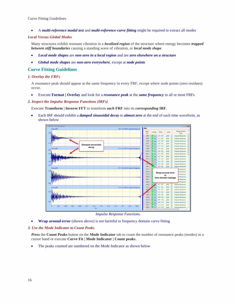
2. Inspect the Impulse Response Functions (IRFs)
Execute Transform | Inverse FFT to transform each FRF into its corresponding IRF.
• Each IRF should exhibit a damped sinusoidal decay to almost zero at the end of each time waveform, as
shown below
Impulse Response Functions.
• Wrap around error (shown above) is not harmful to frequency domain curve fitting
3. Use the Mode Indicator to Count Peaks
Press the Count Peaks button on the Mode Indicator tab to count the number of resonance peaks (modes) in a
cursor band or execute Curve Fit | Mode Indicator | Count peaks.
• The peaks counted are numbered on the Mode Indicator as shown below
17
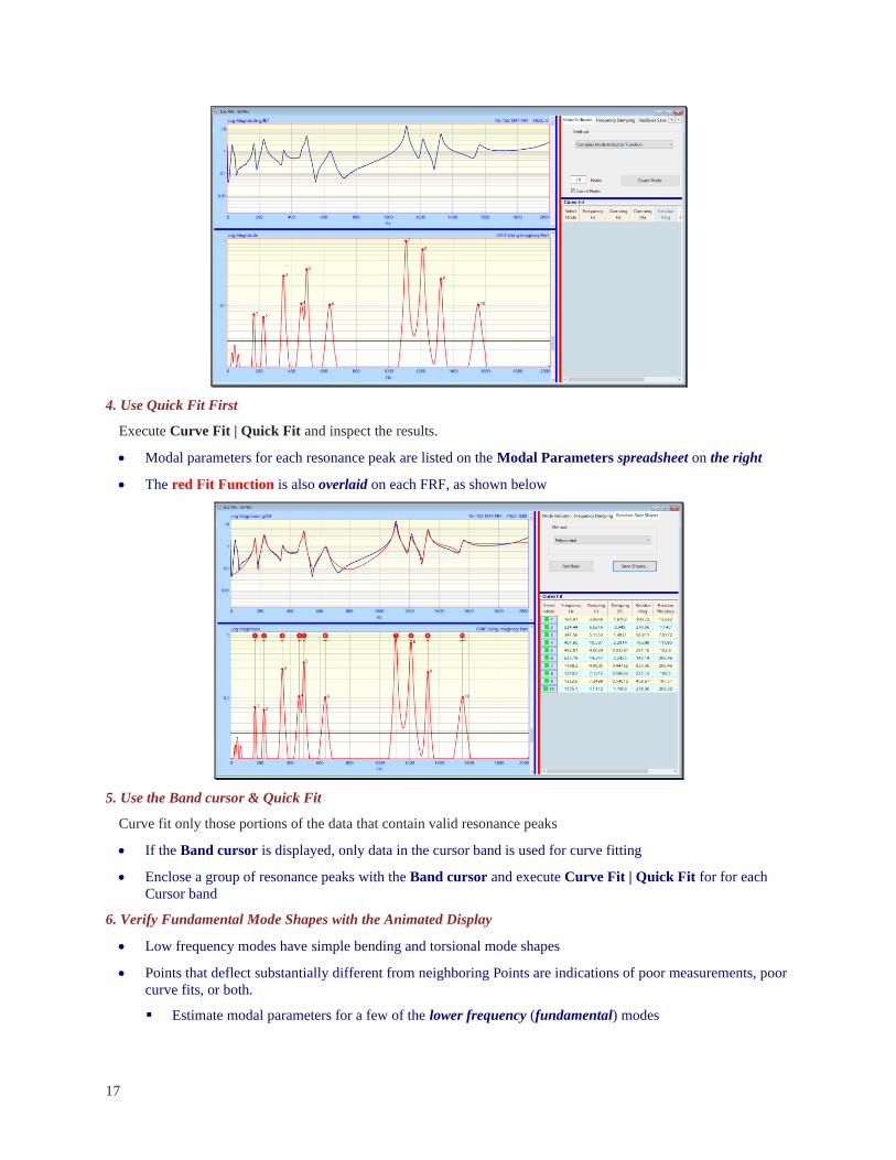
4. Use Quick Fit First
Execute Curve Fit | Quick Fit and inspect the results.
• Modal parameters for each resonance peak are listed on the Modal Parameters spreadsheet on the right
• The red Fit Function is also overlaid on each FRF, as shown below
5. Use the Band cursor & Quick Fit
Curve fit only those portions of the data that contain valid resonance peaks
• If the Band cursor is displayed, only data in the cursor band is used for curve fitting
• Enclose a group of resonance peaks with the Band cursor and execute Curve Fit | Quick Fit for for each
Cursor band
6. Verify Fundamental Mode Shapes with the Animated Display
• Low frequency modes have simple bending and torsional mode shapes
• Points that deflect substantially different from neighboring Points are indications of poor measurements, poor
curve fits, or both.
Estimate modal parameters for a few of the lower frequency (fundamental) modes

Curve Fit | Open Curve Fitting
18
Save the results into a Shape Table (SHP) and display the mode shapes in animation to verify their mode
shapes
7. Compare Results from Different Curve Fitting Methods
• Curve fit the FRFs using more than one curve fitting method
• Compare mode shapes from different methods
Execute Display | MAC (Modal Assurance Criterion) to numerically compare mode shape pairs
Execute Draw | Animate a Pair to display shapes from two different curve fitting methods
Curve Fit | Open Curve Fitting
Enables & disables FRF-based curve fitting in a frequency domain Data Block (BLK).
• When checked, curve fitting is enabled, and the following changes take place in the Data Block (BLK)
window
Data Block (BLK) M#s are displayed on the upper left side of the window
A Mode Indicator graph is displayed on the lower left side of the window
Mode Indicator, Frequency Damping, and Residues Save Shapes tabs are displayed on the upper
right side of the window, separated from the graphics by a vertical red splitter bar
A Modal Parameters spreadsheet is displayed lower right side of the window, separated from the tabs
by a horizontal blue splitter bar
Data Block (BLK) Window during Curve Fitting.
Curve Fitting commands are enabled in the Curve Fit menu
• During curve fitting, four splitter bars are displayed in the Data Block (BLK) window

19
Vertical Splitter Bars
The vertical blue splitter bar separates the M# graphics s & Mode Indicator on the left from the M#s
spreadsheet on the right.
• Drag the vertical blue splitter bar horizontally to display the M#s spreadsheet
The vertical red splitter bar separates the M# graphics and Mode Indicator on the left from the Curve Fitting
tabs and Modal Parameters spreadsheet on the right of the window.
• Drag the vertical red splitter bar horizontally to change the size of the Curve Fitting tabs or the M#
graphics area
Horizontal Splitter Bars
The left horizontal blue splitter bar separates the M#s graph and the Mode Indicator graph.
• Drag the left blue splitter bar vertically to change the size of the M# graphics or the Mode Indicator
The right horizontal blue splitter bar separates the Curve Fitting tabs and the Modal Parameters spreadsheet.
• Drag the right blue splitter bar vertically to change the size of the Curve Fitting tabs or the Modal
Parameters spreadsheet
Modal Parameters Spreadsheet
A list of all modal parameter estimates.
• Each row of this spreadsheet contains modal parameter estimates for one mode
Modal Parameters Spreadsheet
Select Mode Column
• Click on the Select Mode button to toggle the mode selection
• Double click on the Select Mode column heading to toggle the selection of all modes
Frequency & Damping Columns
• The damped natural frequency is listed in the Frequency (Hz) column
• Modal damping can be listed is two columns, either as the half power point damping in the Damping (Hz)
column or as the percent of critical damping in the Damping % column

Curve Fit | Open Curve Fitting
20
Residue Magnitude & Phase Columns
• The Residue for each mode is listed as magnitude & phase
The magnitude units are the FRF units x (radians per second)
If the FRF units are (g/ N), the Residue units are (g/ N-sec)
• Phase units are in degrees
Methods Columns
• The Frequency Damping Method column lists the curve fitting methods used to estimate frequency &
damping of each mode and the frequency band of data used
• The Residue Method column lists the curve fitting method used to estimate the Residue of each mode and
the frequency band of data used
Showing & Hiding Spreadsheet Columns
All spreadsheet columns can be shown or hidden, except the Select Mode column.
• Right click on any spreadsheet and select Show Hide Columns from the menu
The File | Data Block Options box will open displaying the Show Hide tab
Check columns to show them and un-check columns to hide them
Default Spreadsheet Column Widths
• Right click on any spreadsheet and execute Reset Column Widths to set its default column width
Spreadsheet Text Cells
• Select the text in one or more spreadsheet cells
• Hold down the Ctrl key and
Press the X key to cut the selected text to the Clipboard
Press the C key to copy the selected text to the Clipboard
Press the V key to paste text from the Clipboard into the selected cells

21
Mode Indicator Tab
The first step of modal parameter estimation is to determine how many modes are represented by resonance peaks
in a set of measurements.
• The Mode Indicator tab is used to
Calculate a Mode Indicator function
Count the peaks above a Noise Threshold Line on the Mode Indicator, as shown below
Mode Indicator Tab
• The Peaks box on the Mode Indicator tab contains the number of peaks counted
To calculate the Mode Indicator function and count its peaks,
• Choose an Indicator from the Method list on the Mode Indicator tab
• Press the Count Peaks button or execute Curve Fit | Mode Indicator | Count Peaks
A dialog box will open for choosing a part of the M# data to use for calculating the Mode Indicator.
Choose the Imaginary part if the FRFs have response units of Displacement or Acceleration
Choose the Real part if the FRFs have response units of Velocity
Choose Magnitude for all other types of M#s
After the Mode Indicator is calculated, its peaks are counted above the horizontal noise threshold line.
• Each modal peak is indicated on the Mode Indicator graph with a red dot and a number next to it
• The number of peaks counted is displayed in the Peaks box
• Resonance peaks are counted on the Mode Indicator when
The Band cursor is moved
The noise threshold is scrolled

Frequency & Damping Curve Fitting Methods
22
A new Mode Indicator is calculated
Curve Fit | Mode Indicator | Smooth Indicator is executed to smooth the Mode Indicator
Frequency & Damping Curve Fitting Methods
Polynomial Method
The Polynomial method is Multi-Degree-Of-Freedom (MDOF) method that simultaneously estimates the
modal parameters of one or more modes.
• A least squared error curve fit is performed on the FRF data to obtain estimates of the coefficients of the
FRF denominator polynomial, called the characteristic polynomial.
• Modal frequency & damping estimates are then extracted as the roots of the characteristic polynomial.
Global Curve Fitting
Each resonance peak in an FRF is evidence of at least one mode
• All FRF measurements taken from the same structure should have a resonance peak at the same frequency
for each resonance
• If multiple FRFs are overlaid, each resonance peak should appear at the same frequency in all FRFs
Non-Stationary Data
If multiple FRFs are acquired under non-stationary conditions (different mass loading due to roving
accelerometers, temperature changes, etc.), when the FRFs are overlaid, the resonance peaks for a mode may not
line up at the same frequency.
Global Versus Local Curve Fitting
Global curve fitting can be used when resonance peaks line up at the same frequency in a set of overlaid FRFs.
Local curve fitting should be used when resonance peaks do not line up at the same frequency in a set of overlaid
FRFs.
Frequency Damping Tab
Contains curve fitting methods for estimating the modal frequency & damping of each resonance peak in the
FRFs.
• If Count Peaks was checked, the number of modes in the Modes box is the same as the number of peaks
counted in the Peaks box on the Mode Indicator tab
• When the Frequency Damping button is pressed or Curve Fit | Frequency Damping | Frequency
Damping is executed, the current Method chosen on the tab is used to calculate estimates for the number of
modes in the Modes box
• All modal frequency & damping estimates are added to the Modal Parameters spreadsheet
Global Polynomial Method
Estimates a global value of frequency & damping for each mode from all FRFs
Local Polynomial Method
Estimates a local value of frequency & damping for each mode from each FRF

23
Frequency & Damping Estimates for Six Modes.
Vertical Frequency Lines
Each frequency estimate in the Modal Parameters spreadsheet is displayed as a vertical blue line on the Mode
Indicator
If a mode is selected, a vertical red line is displayed at each modal frequency on the Mode Indicator
In the Band cursor is displayed, the modes in the band are selected
Horizontal Damping Lines
Each modal damping estimate is displayed as a horizontal blue line crossing at the top of the vertical frequency
line.
The length of the horizontal blue line is twice the modal damping (2σ)
σ is called the half power point damping (Hz), the 3 dB point damping, or the damping decay constant
2 σ is approximately equal to the width of the resonance peak at 70.7 % of the FRF peak magnitude, or
half of the peak magnitude squared
• Spin the mouse wheel to Zoom In and display the horizontal damping lines more clearly
Residue Curve Fitting Methods
24
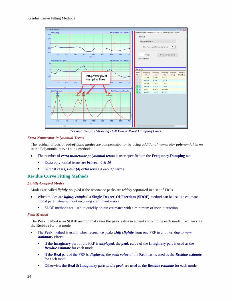
Zoomed Display Showing Half Power Point Damping Lines.
Extra Numerator Polynomial Terms
The residual effects of out-of-band modes are compensated for by using additional numerator polynomial terms
in the Polynomial curve fitting methods.
• The number of extra numerator polynomial terms is user-specified on the Frequency Damping tab
Extra polynomial terms are between 0 & 10
In most cases, Four (4) extra terms is enough terms
Residue Curve Fitting Methods
Lightly-Coupled Modes
Modes are called lightly-coupled if the resonance peaks are widely separated in a set of FRFs.
• When modes are lightly-coupled, a Single-Degree-Of-Freedom (SDOF) method can be used to estimate
modal parameters without incurring significant errors
SDOF methods are used to quickly obtain estimates with a minimum of user interaction
Peak Method
The Peak method is an SDOF method that saves the peak value in a band surrounding each modal frequency as
the Residue for that mode
• The Peak method is useful when resonance peaks shift slightly from one FRF to another, due to non-
stationary effects
If the Imaginary part of the FRF is displayed, the peak value of the Imaginary part is used as the
Residue estimate for each mode
If the Real part of the FRF is displayed, the peak value of the Real part is used as the Residue estimate
for each mode
Otherwise, the Real & Imaginary parts at the peak are used as the Residue estimate for each mode

25
Lightly Coupled and Closely Coupled Modes
Closely Coupled Modes
Modes are called closely-coupled if two or more modes are represented by closely-spaced resonance peaks in a
set of FRFs.
• A Multi-Degree-Of-Freedom (MDOF) method should be used to simultaneously estimate the modal
parameters of closely-coupled modes
Polynomial Method
When the polynomial method is used for Residue curve fitting, the numerator polynomial is estimated by a least
squared error curve fitting process on each FRF.
• Following the curve fitting process, the Residue estimate for each mode is obtained by performing a partial
fraction expansion of each numerator polynomial
Extra Numerator Polynomial Terms
When the polynomial method is used for Residue curve fitting, the residual effects of out-of-band modes are
compensated for by using additional numerator polynomial terms.
• The number of extra polynomial terms is specified on the Frequency Damping tab
Residues Save Shapes Tab
When the Residues button is pressed, the curve fitting method chosen from the Methods list is used to estimate a
complex Residue (magnitude & phase) for each mode and each FRF.
• All (or selected) FRFs are curve fit for all (or selected) modes in the Modal Parameters spreadsheet
• The Residue estimates for all (or selected) modes are added to the Modal Parameters spreadsheet
Fit Function
After residues are estimated, a red fit function is synthesized using all the modal parameters.
• Each red fit function is overlaid on each M# in the upper left graphics area
Each red fit function should closely match its corresponding FRF over the curve fitting band

Residues Save Shapes Tab
26
Curve Fitting After Residues Have Been Estimated.
• If it is displayed, use the vertical scroll bar next to the M# graphics to display each FRF, its red fit
function, and its modal parameters in the Modal Parameters spreadsheet
• Use several different display formats (Magnitude, Bode, Nyquist) to compare the FRF and its red fit
function
Save Shapes Button
This button is enabled when at least one mode has a Residue estimate listed in the Modal Parameters
spreadsheet.
• When the Save Shapes button is pressed, modal parameters for all (or selected) modes and all (or selected)
M#s are saved into a Shape Table (SHP)
Exponential Window Damping Removal
If an exponential window was applied to the FRFs, each modal damping estimate will have an amount of
artificial damping added to it.
• When modal parameters are saved into a Shape Table (SHP), the amount of artificial damping is subtracted
from all modal damping estimates
• The amount of artificial damping due to exponential windowing is displayed in the Window Value column
of the M#s spreadsheet
Residue mode shapes
When the Save Shapes button is pressed, Residue mode shapes are saved into the Shape Table (SHP)
• A set of Residue mode shapes estimated from calibrated FRFs is called a Modal Model
A Modal Model preserves the dynamic properties (mass, stiffness, & damping) of the structure and can
be used for a variety of analyses.

27
Curve Fitting OMA Measurements
Operational Modal Analysis (OMA) is the process of extracting modal parameters (called operating mode
shapes) from a set of output-only measurements
Output-only Measurements
Fourier spectra, Cross spectra & ODS FRFs can be calculated from output only, response only, or operating data
where the excitation forces are not measured.
Flat Force Spectrum
FRF-based curve fitting is applied mainly around the resonance peaks in a Fourier spectrum, Cross spectrum, or
ODS FRF.
ASSUMPTION: If the frequency spectrum of the un-measured excitation forces is assumed to be relatively flat
around each resonance peak, then operating mode shapes can be extracted from output-only measurements using
FRF-based curve fitting methods.
Curve Fitting Fourier Spectra
A Fourier spectrum is the FFT of single channel time waveform
• If all response time waveforms are simultaneously acquired, then operating mode shapes can be extracted
from a set of Fourier spectra using FRF-based curve fitting methods
Curve Fitting Cross Spectra
A Cross spectrum is a cross channel measurement that is calculated between two channels of response data.
• After a DeConvolution window has been applied to a set of Cross spectra, operating mode shapes can be
extracted from them using FRF-based curve fitting methods
• Multiple Measurement Sets of Cross spectra can be calculated from one or more simultaneously acquired
Roving responses and the same fixed Reference response, and curve fit using FRF-based curve fitting
methods
Curve Fitting ODS FRFs
An ODS FRF is a hybrid cross channel measurement, the magnitude of which is the Auto spectrum of a Roving
response and the phase of which is from the Cross spectrum between the Roving and a fixed Reference response.
• The correct relative phase between all Roving responses is preserved if all ODS FRFs are calculated using
the same fixed Reference response
• After a DeConvolution window has been applied to a set of ODS FRFs, operating mode shapes can be
extracted from them using FRF-based curve fitting methods
• Multiple Measurement Sets of ODS FRFs can be calculated from one or more simultaneously acquired
Roving responses and the same fixed Reference response

Data Block (BLK) Curve Fit Menu
28
Data Block (BLK) Curve Fit Menu
Curve Fit | Quick Fit
Curve fits all (or selected) M#s using the currently selected methods on the Mode Indicator, Frequency Damping,
and Residues Save Shapes tabs.
• If the Band cursor is displayed, only the data in the band is used for curve fitting
Quick Fit Steps
• If no Mode Indicator is displayed, a Mode Indicator is calculated using the current Method on the Mode
Indicator tab
• Peaks above the noise threshold line on the Mode Indicator are counted
• Modal Frequency & Damping are estimated for the number of peaks counted, using the current Method on
the Frequency Damp tab
• Modal Residues are estimated for the modes estimated in the previous step, using the current Method on the
Residues Save Shapes tab
• A red Fit Function is synthesized and overlaid on the experimental FRF data
Improving Quick Fit Results
• If some Quick Fit results are not satisfactory,
Execute Curve Fit | Modal Parameters | Delete Modes to remove the selected modes from the Modal
Parameters spreadsheet
Display the Band cursor or change its position to surround fewer resonance peaks
Execute Curve Fit | Mode Indicator | Smooth Indicator to remove noise peaks from the Mode
Indicator
Scroll the noise threshold line on the Mode Indicator so that only resonance peaks are counted
Execute Curve Fit | Quick Fit again
Data Block (BLK) Window Following a Quick Fit in Four Bands.

29
Count Peaks Un-Checked
Quick Fit estimates modal parameters for the number of modes in the Modes box on the Frequency Damping
tab.
• To estimate Frequency & Damping for a fixed number of modes
Un-check the Count Peaks box on the Frequency Damp tab
Enter a number into the Modes box
Execute Curve Fit | Quick Fit or press the Frequency Damping button
Curve Fit | Delete All Fit Data
All curve fitting data is saved with the Data Block (BLK) in which curve fitting was performed. Before starting a
new session of curve fitting, it is a good practice to delete all curve fitting data from the Data Block (BLK).
• When this command is executed, the following data is deleted,
All modal parameters in the Modal Parameters spreadsheet
All Fit Functions
All Mode Indicators
Curve Fit | Mode Indicator | Count Peaks
Calculates a Mode Indicator, counts its peaks above the noise threshold line on a Mode Indicator graph, and sets
the number peaks counted in the Peaks box.
• Executing this command is the same as pressing the Count Peaks button on the Mode Indicator tab
Curve Fit | Mode Indicator | Clear Indicator
Clears (zeroes) the Mode Indicator in the lower left graphics area.
• The Mode Indicator is used by the Polynomial methods on the Frequency Damping tab
• If the Band cursor is displayed, the Mode Indicator is cleared in the cursor band
Curve Fit | Mode Indicator | Smooth Indicator
Smooths the Mode Indicator to remove noise peaks.
• An exponential window is applied to the Mode Indicator to smooth it
See Transform | Window Data | Exponential command for details

Data Block (BLK) Curve Fit Menu
30
• Each time this command is executed, more noise peaks are removed from the Mode Indicator, but the
resonance peaks will become wider
Curve Fit | Mode Indicator | CMIFs
Calculates and displays the Complex Mode Indicator Functions (CMIFs) in Mode Indicator area of the Data
Block (BLK) window.
Curve Fit | Mode Indicator | MMIFs
Calculates and displays the Multivariate Mode Indicator Functions (MMIFs) in Mode Indicator area of the
Data Block (BLK) window.
Curve Fit | Mode Indicator | Copy CMIFs
Copies the CMIFs (including their Modal Participation curves) into another Data Block (BLK).
• This command is enabled when not curve fitting
Curve Fit | Mode Indicator | Copy MMIFs
Copies the MMIFs (including their Modal Participation curves) into another Data Block (BLK).
• This command is enabled when not curve fitting
Curve Fit | Frequency Damping | Number of Modes
Sets the number of modes to be used by the Frequency Damping curve fitting methods.
Curve Fit | Frequency Damping | Frequency Damping
Estimates modal frequency & damping for the current number in the Modes box on the Frequency Damping
tab, using all (or current Band cursor) data from all (or selected) M#s in the Data Block (BLK).
Curve Fit | Residues
Estimates modal residues using all (or selected) modes in the Modal Parameters spreadsheet, using data from all
(or selected) M#s in the Data Block (BLK).
• Executing this command is the same as pressing the Residues button on the Residues Save Shapes tab
Curve Fit | Modal Parameters | Sort by Frequency
Sorts the modes in the Modal Parameters spreadsheet by ascending order of frequency.
Curve Fit | Modal Parameters | Select All Modes, Select None, Invert Selection
These commands are used for selecting modes in the Modal Parameters spreadsheet
Curve Fit | Modal Parameters | Delete Modes
Deletes the selected modes from the Modal Parameters spreadsheet.
Curve Fit | Modal Parameters | Save Shapes
Saves all (or selected) modes from the Modal Parameters into a Shape Table (SHP).
• This command is the same as pressing the Save Shapes button on the Residues Save Shapes tab
Curve Fit | Modal Parameters | MAC
Opens the Modal Assurance Criterion (MAC) window for comparing shapes in the Modal Parameters
spreadsheet with shapes in a chosen Shape Table (SHP).
Curve Fit | Fit Functions | Clear Fit Functions
Clears (zeros) the red Fit Functions of all (or selected) M#s.
• If the Band cursor is displayed, the Fit Functions are cleared in the band

31
Curve Fit | Fit Functions | Synthesize Fit Functions
Synthesizes a red Fit Function for all (or selected) M#s, using the modal parameters of all (or selected) modes in
the Modal Parameters spreadsheet.
• A red Fit Function is overlaid on each M#
• If the Band cursor is displayed, Fit Functions are synthesized in the band
Synthesized Fit Function Overlaid on an FRF.
Curve Fit | Fit Functions | Fit Functions
Toggles the display of the Fit Functions overlaid on the FRFs in the Data Block (BLK) window.
• This command is enabled when not curve fitting
Curve Fit | Fit Functions | Copy Fit Functions
Copies the Fit Functions into another Data Block (BLK).
• This command is enabled when not curve fitting
Curve Fit | Close Curve Fitting
Terminates curve fitting and removes the Curve Fitting tabs from the Data Block (BLK) window

Shape Table (SHP) Display Menu
32
Shape Table (SHP) Display Menu
Display | MAC
Calculates and displays Modal Assurance Criterion (MAC) values between pairs of shapes in two Shape Tables
(SHPs)
• Each Shape Table (SHP) can contain ODS's, EMA Mode Shapes, FEA Mode Shapes, or Engineering Data
Shapes
What is MAC?
MAC is a quantitative method for comparing two shape vectors, u & v.
• MAC is calculated between two shapes u & v with the formula
u complex shape (m-vector)
v complex shape (m-vector)
m the number of matching DOFs
h transposed conjugate vector
|| ||2 magnitude squared of the vector product
• MAC values range between 0 & 1
MAC = 1.00 two shapes are co-linear, they both lie on the same straight line
MAC > 0.90 two shapes are similar
MAC < 0.90 two shapes are different
MAC 3D Bar Chart.

33
• Only shape components with matching DOFs in the two Shape Tables (SHPs) are used to calculate MAC
values
What is CoMAC?
Coordinate Modal Assurance Criterion (CoMAC) is a quantitative method for comparing shape components or
shape DOFs between pairs of shapes in two Shape Tables (SHPs).
• Each Shape Table (SHP) can contain ODS's, FEA Mode Shapes, EMA Mode Shapes, or Engineering Data
Shapes.
• CoMAC uses the same formula as MAC, but u & v are vectors of data from two M#s with matching
DOFs
• CoMAC values range between 0 & 1
CoMAC = 1.00 components of all (or selected) shapes are co-linear for a pair of matching DOFs
CoMAC > 0.90 components of all (or selected) shapes are similar for a pair of matching DOFs
CoMAC < 0.90 components of all (or selected) shapes are different for a pair of matching DOFs
MAC Window Commands
File | Copy Graphics to Clipboard
Copies the MAC window graphics to the Windows Clipboard.
File | Print
Prints the graphics on the system graphics printer.
File | Close
Closes the MAC window.
Display | Spreadsheet
Displays the MAC or CoMAC values in a spreadsheet.
Display | 3D Bar Chart
Displays the MAC or CoMAC values in a 3D bar chart.
• Right click & drag to rotate the 3D Bar Chart
Display | Values
When checked, the MAC or CoMAC value for one shape pair is displayed on the 3D Bar Chart.
• Hover the mouse pointer over a bar to display its value
Display | MAC, CoMAC
When checked, either MAC or CoMAC values are displayed in either a 3D Bar Chart or a spreadsheet.

Shape Table (SHP) Display Menu
34
Structure Options Animation Tab
If Show MAC is checked on the Animation tab in the File | Structure Options box, the MAC value between
two shapes is displayed during animation of a pair of shapes.
Display | SDI
Opens the Shape Difference Indicator (SDI) window from a Shape Table (SHP).
• Each Shape Table (SHP) can contain ODS's, EMA Mode Shapes, FEA Mode Shapes, or Engineering Data
Shapes.
What is SDI?
SDI is a quantitative measure of the difference between two shape vectors u & v.
• SDI is calculated between two shapes u & v using the formula
real(uhv) real part of the vector product
u complex shape (m-vector)
v complex shape (m-vector)
m the number of matching DOFs
h transposed conjugate vector
35
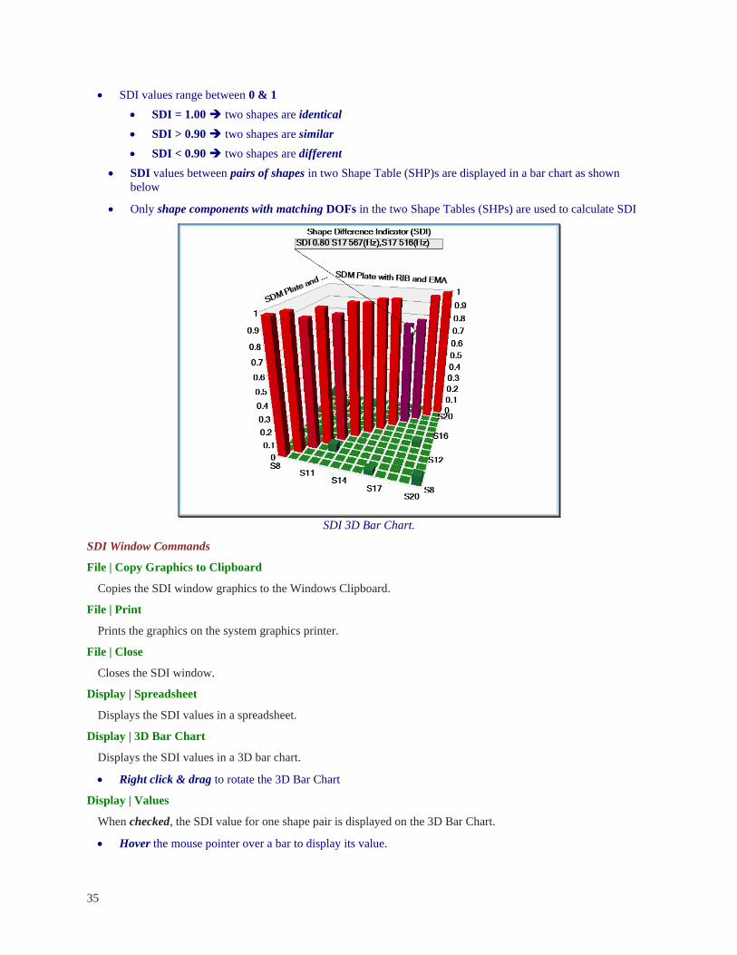
• SDI values range between 0 & 1
• SDI = 1.00 two shapes are identical
• SDI > 0.90 two shapes are similar
• SDI < 0.90 two shapes are different
• SDI values between pairs of shapes in two Shape Table (SHP)s are displayed in a bar chart as shown
below
• Only shape components with matching DOFs in the two Shape Tables (SHPs) are used to calculate SDI
SDI 3D Bar Chart.
SDI Window Commands
File | Copy Graphics to Clipboard
Copies the SDI window graphics to the Windows Clipboard.
File | Print
Prints the graphics on the system graphics printer.
File | Close
Closes the SDI window.
Display | Spreadsheet
Displays the SDI values in a spreadsheet.
Display | 3D Bar Chart
Displays the SDI values in a 3D bar chart.
• Right click & drag to rotate the 3D Bar Chart
Display | Values
When checked, the SDI value for one shape pair is displayed on the 3D Bar Chart.
• Hover the mouse pointer over a bar to display its value.
Shape Table (SHP) Display Menu
36
Structure Options Animation Tab
If Show SDI is checked on the Animation Tab in the File | Structure Options box, the SDI value between two
shapes is displayed during animation of a pair of shapes.
Display | Participation
Displays Participation values between pairs of shapes in two Shape Tables (SHPs).
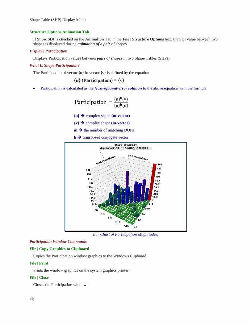
What Is Shape Participation?
The Participation of vector u in vector v is defined by the equation
u (Participation) = v
• Participation is calculated as the least-squared-error solution to the above equation with the formula
u complex shape (m-vector)
v complex shape (m-vector)
m the number of matching DOFs
h transposed conjugate vector
Bar Chart of Participation Magnitudes.
Participation Window Commands
File | Copy Graphics to Clipboard
Copies the Participation window graphics to the Windows Clipboard.
File | Print
Prints the window graphics on the system graphics printer.
File | Close
Closes the Participation window.

37
Display | Spreadsheet
Displays the Participation values in a spreadsheet.
Display | 3D Bar Chart
Displays the Participation values in a 3D bar chart.
• Right click & drag to rotate the 3D Bar Chart
Display | Value
When checked, the Participation value for one shape pair is displayed on the 3D Bar Chart.
• Hover the mouse pointer over a bar to display its value
Display | Real Part, Imaginary Part, Magnitude
When checked, displays the Real Part, Imaginary Part or Magnitude of the Participation values in either a 3D Bar
Chart or a spreadsheet.
Shape Table (SHP) Tools Menu
Tools | Synthesize FRFs
When this command is executed, a dialog box will open allowing you to choose a Shape Table (SHP) with a
Modal Model in it
• If using Residue mode shapes, choose all desired DOFs for synthesizing FRFs
• If using UMM mode shapes, choose all desired Roving & Reference DOFs for synthesizing FRFs
Residue mode shapes
Residue mode shapes are obtained from curve fitting a set of FRFs
• Each component of a Residue mode shape is defined between a pair of DOFs (Roving DOF : Reference
DOF)
UMM mode shapes
UMM mode shapes can be obtained from an FEA model or by re-scaling a set of Residue mode shapes
• FRFs can be synthesized for any two M#s in a set of UMM mode shapes

Shape Table (SHP) Tools Menu
38
Type of Shapes in a Shape Table (SHP) FRFs Synthesized
Residue mode shapes Only for each shape component
UMM mode shapes Between any pair of shape
components
What is a Modal Model?
Both Residue mode shapes and UMM mode shapes are called a Modal Model when they are scaled in a manner
which preserves the dynamic properties of a structure (its mass, stiffness, & damping properties).
• The mode shapes of a Modal Model can be used for
Synthesizing FRFs
MIMO calculation of multiple Outputs from multiple Inputs, and multiple Inputs from multiple Outputs
SDM including Modal Sensitivity, Sub structuring, Adding Tuned Absorbers
FEA Model Updating
Overlaying Synthesized & Measured FRFs
• Select the measured FRFs in their Data Block (BLK)
• In the Data Block (BLK) window containing the synthesized FRFs, execute Edit | Paste M#s from File to
paste the measured FRFs together with the synthesized FRFs
• Use the Color column in the M#s spreadsheet to color the synthesized FRFs and measured FRFs differently
• Execute Format | Overlay by DOF to overlay the synthesized & measured FRFs
Synthesized &Measured FRFs Overlaid.
39
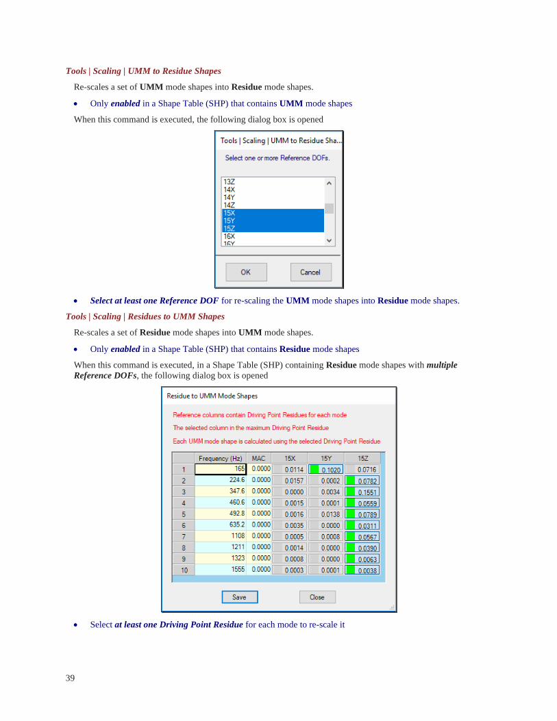
Tools | Scaling | UMM to Residue Shapes
Re-scales a set of UMM mode shapes into Residue mode shapes.
• Only enabled in a Shape Table (SHP) that contains UMM mode shapes
When this command is executed, the following dialog box is opened
• Select at least one Reference DOF for re-scaling the UMM mode shapes into Residue mode shapes.
Tools | Scaling | Residues to UMM Shapes
Re-scales a set of Residue mode shapes into UMM mode shapes.
• Only enabled in a Shape Table (SHP) that contains Residue mode shapes
When this command is executed, in a Shape Table (SHP) containing Residue mode shapes with multiple
Reference DOFs, the following dialog box is opened
• Select at least one Driving Point Residue for each mode to re-scale it

Shape Table (SHP) Tools Menu
40
Tools | Scaling | Un-Scaled to Scaled Shapes
Re-scales a set of un-scaled shapes using a set of Residue mode shapes or UMM mode shapes.
• This command is useful for re-scaling OMA mode shapes using the following scaled mode shapes
FEA mode shapes that are scaled as Residue mode shapes or UMM mode shapes
EMA mode shapes that are scaled as Residue mode shapes or UMM mode shapes
Tools | Scaling | Rapid Test Residues to UMM Shapes
Re-scales a set of Rapid Test Residues to UMM mode shapes.
What is a Rapid Test?
Rapid Test Residues are obtained by curve fitting a set of measurements that were calculated from a TRN chain
of acquired data.
• In a Rapid Test, either the impactor or the response sensor (e.g. the accelerometer) can be moved between
acquisitions of data, provided that a TRN chain of data is acquired.
A TRN chain is formed when each Measurement Set of acquired data contains a DOF that is also
contained in another Measurement Set


