

Louisiana State UniversityLSU Digital Commons
LSU Master's Theses Graduate School
11-10-2017
Microgrid Energy Management with FlexibilityConstraints: A Data-Driven Solution MethodOkan CiftciLouisiana State University and Agricultural and Mechanical College, [email protected]
Follow this and additional works at: https://digitalcommons.lsu.edu/gradschool_theses
Part of the Power and Energy Commons
This Thesis is brought to you for free and open access by the Graduate School at LSU Digital Commons. It has been accepted for inclusion in LSUMaster's Theses by an authorized graduate school editor of LSU Digital Commons. For more information, please contact [email protected].
Recommended CitationCiftci, Okan, "Microgrid Energy Management with Flexibility Constraints: A Data-Driven Solution Method" (2017). LSU Master'sTheses. 4351.https://digitalcommons.lsu.edu/gradschool_theses/4351

MICROGRID ENERGY MANAGEMENT WITH FLEXIBILITY
CONSTRAINTS: A DATA-DRIVEN SOLUTION METHOD
A Thesis
Submitted to the Graduate Faculty of the
Louisiana State University and
Agricultural and Mechanical College
in partial fulfillment of the
requirements for the degree of
Master of Science in Electrical Engineering
in
The School of Electrical Engineering and Computer Science
by
Okan Ciftci
B.S., KTO Karatay University, Konya, Turkey, 2014
December 2017

ii
to my family

iii
ACKNOWLEDGMENTS
I would like to first express all my deepest respect and appreciation to my academic advisor,
Dr. Amin Kargarian, for his continuous support to earn my degree. I thank him for guiding me
with his patience and immense knowledge. He was more than an advisor to me from beginning to
the end. He was always kind, motivator, and supporter at everything, even in my daily life. Nothing
is enough to express my sincere respect to him.
I would like to thank Dr. Mehraeen, and Dr. Czarnecki who taught graduate level courses, and
Dr. Farasat who was one of the committee members.
I want to express my deepest appreciation to Turkish Government who supports me financially
in US to receive Master’s and PhD education.
Above all, I am deeply grateful to my parents, Necati and Gulduran Ciftci, and my brothers,
Sadettin and Arif. Their love has sustained me. My mother and father have stood by me all the
time here. My brothers always supported me, thank you so much. I could not have done this work
without you’re the love of my family.
iv
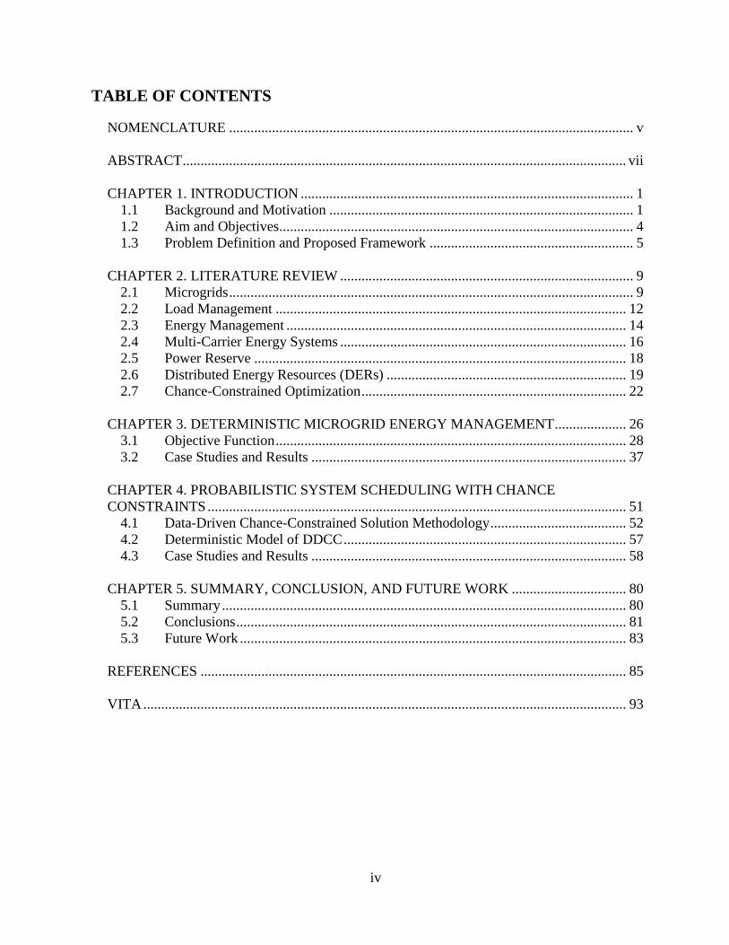
TABLE OF CONTENTS
NOMENCLATURE ................................................................................................................. v
ABSTRACT ............................................................................................................................ vii
CHAPTER 1. INTRODUCTION ............................................................................................. 1
1.1 Background and Motivation ..................................................................................... 1 1.2 Aim and Objectives................................................................................................... 4 1.3 Problem Definition and Proposed Framework ......................................................... 5
CHAPTER 2. LITERATURE REVIEW .................................................................................. 9
2.1 Microgrids ................................................................................................................. 9
2.2 Load Management .................................................................................................. 12
2.3 Energy Management ............................................................................................... 14 2.4 Multi-Carrier Energy Systems ................................................................................ 16
2.5 Power Reserve ........................................................................................................ 18 2.6 Distributed Energy Resources (DERs) ................................................................... 19
2.7 Chance-Constrained Optimization .......................................................................... 22
CHAPTER 3. DETERMINISTIC MICROGRID ENERGY MANAGEMENT .................... 26
3.1 Objective Function .................................................................................................. 28 3.2 Case Studies and Results ........................................................................................ 37
CHAPTER 4. PROBABILISTIC SYSTEM SCHEDULING WITH CHANCE
CONSTRAINTS ..................................................................................................................... 51 4.1 Data-Driven Chance-Constrained Solution Methodology ...................................... 52
4.2 Deterministic Model of DDCC ............................................................................... 57 4.3 Case Studies and Results ........................................................................................ 58
CHAPTER 5. SUMMARY, CONCLUSION, AND FUTURE WORK ................................ 80 5.1 Summary ................................................................................................................. 80
5.2 Conclusions ............................................................................................................. 81 5.3 Future Work ............................................................................................................ 83
REFERENCES ....................................................................................................................... 85
VITA ....................................................................................................................................... 93

v
NOMENCLATURE
Parameters:
a CHP fuel consumption coefficient for electricity production
b CHP fuel consumption coefficient at minimum output of thermal energy
Cb Cost of operation of battery
Cfg Cost of power buying from the distribution feeder
Cgas Cost of natural gas
Ctg Cost of power selling to the distribution feeder
E(⋅) Expected value
Hboimin, Hboi
max Minimum and maximum boundaries of thermal power generated by boiler
Hchp,rd, Hchp,ru Ramping up and down rates of CHP for thermal power generation
M𝑔𝑓 , Mgt Upper limits for electric power exchanged between MG and the
distribution feeder
Minone, Minonh Minimum continuous operating time intervals for controllable loads
Pbcmax, Pbd
max Maximum charging and discharging power limits of battery
Pbrd, Pbru Ramping up and down rates, which are assessed by the system operator
Pchpmin, Pchp
max Minimum and maximum limits of electrical power generated by CHP
Pchp,rd, Pchp,ru Ramping up and down rates of CHP for electrical power generation
Pcn,tmin, Hcn,t
min Minimum limits of controllable electrical and thermal load
Pvg,tmax Maximum limit of virtual power generation output
RNG𝑒, RNGℎ Range of controllable load intervals
Smin, Smax Minimum and maximum limits of state of charge of battery
Si, Sf Predefined value for the initial and final state of charge of battery
T Time horizon
T𝑒on, Th
on Minimum continuous operating period for controllable loads
Δt Time resolution (which is 5 minutes in this thesis)

vi
ηbc, ηbd Efficiency of battery charging and discharging
ηboi Efficiency of boiler
ηhc Efficiency of thermal coil
ηhr Thermal recovery efficiency of combined heat and power
ϖ, ω Required regulation reserve for solar and load
F̂(⋅)−1 Inverse cumulative distribution function (CDF)
Decision Variables:
𝐹𝑏𝑜𝑖 Boiler’s fuel power consumption
𝐹𝑐ℎ𝑝 CHP’s fuel power consumption
𝐻𝑏𝑜𝑖 Thermal power of the boiler
𝐼𝑐ℎ𝑝, 𝐼𝑏𝑜𝑖,𝑡 The status of CHP and boiler
𝐼𝑐𝑛𝑒, 𝐼𝑐𝑛ℎ The status of controllable electrical and thermal loads
𝐼𝑒 Controllable electrical load indicator
𝐼𝑓𝑔, 𝐼𝑡𝑔 The status of selling to and buying from the distribution feeder
𝐼ℎ Controllable thermal load indicator
𝑃𝑏𝑐, 𝑃𝑏𝑑 Charging and discharging powers of battery
𝑃𝑏𝑑𝑟𝑟, 𝑃𝑏𝑐
𝑟𝑟 Regulation reserve capability for battery discharging and charging
𝑃𝑐ℎ𝑝, 𝐻𝑐ℎ𝑝 Electrical and thermal power generated by CHP
𝑃𝑐𝑛𝑡, 𝐻𝑐𝑛 Controllable electrical and thermal loads
𝑃𝑓𝑔, 𝑃𝑡𝑔 Power buying to and selling from the distribution feeder
𝑃𝑣𝑔 Virtual source power output
𝑆 State of charge of battery
𝑆𝑜𝑙 Solar power (dummy decision variable)
Random Variables:
�̃�𝑛𝑐 Non-controllable thermal loads
�̃�𝑛𝑐 Non-controllable electrical loads
�̃�𝑠𝑜𝑙 Solar power generation
vii
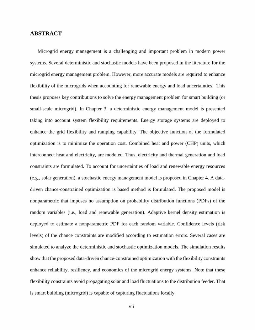
ABSTRACT
Microgrid energy management is a challenging and important problem in modern power
systems. Several deterministic and stochastic models have been proposed in the literature for the
microgrid energy management problem. However, more accurate models are required to enhance
flexibility of the microgrids when accounting for renewable energy and load uncertainties. This
thesis proposes key contributions to solve the energy management problem for smart building (or
small-scale microgrid). In Chapter 3, a deterministic energy management model is presented
taking into account system flexibility requirements. Energy storage systems are deployed to
enhance the grid flexibility and ramping capability. The objective function of the formulated
optimization is to minimize the operation cost. Combined heat and power (CHP) units, which
interconnect heat and electricity, are modeled. Thus, electricity and thermal generation and load
constraints are formulated. To account for uncertainties of load and renewable energy resources
(e.g., solar generation), a stochastic energy management model is proposed in Chapter 4. A data-
driven chance-constrained optimization is based method is formulated. The proposed model is
nonparametric that imposes no assumption on probability distribution functions (PDFs) of the
random variables (i.e., load and renewable generation). Adaptive kernel density estimation is
deployed to estimate a nonparametric PDF for each random variable. Confidence levels (risk
levels) of the chance constraints are modified according to estimation errors. Several cases are
simulated to analyze the deterministic and stochastic optimization models. The simulation results
show that the proposed data-driven chance-constrained optimization with the flexibility constraints
enhance reliability, resiliency, and economics of the microgrid energy systems. Note that these
flexibility constraints avoid propagating solar and load fluctuations to the distribution feeder. That
is smart building (microgrid) is capable of capturing fluctuations locally.

1
CHAPTER 1. INTRODUCTION
Background and Motivation
According to the U.S. Department of Energy (DOE), almost 40% of produced energy is used
in buildings; where residential buildings consume 22%, and commercial buildings use
approximately 18%. In terms of electrical energy, 75% of electricity production in the U.S. is
needed to operate the buildings, and it is projected that to be increased in the next decades [1].
These percentages are reasonably noteworthy to draw our attention to manage energies at the
distribution grid level, close to load centers.
The penetration of distributed energy resources (DERs) in distribution network has been
increasing since a few past decades. This has brought the concept of active distribution grids and
microgrids (MGs). An MG is a low voltage distribution network that includes a group of loads,
DERs, and storage devices. In addition, an MG has an energy management system that monitors
and controls DGs and loads [2-5]. Various types of energies, such as electrical and thermal, might
be managed in MGs. A microgrid in which multiple types of energies are managed together can
be called an energy hub or multi-carrier energy system [6]. In this thesis, we considered a microgrid
(or energy hub or multi-carrier energy system) in which thermal and electrical energies are
management together. Electrical power resources include the distribution feeder (the main
transmission/distribution grid), microturbines, photovoltaic (PV) cells, combined heat and power
(CHP), battery storage, etc., and thermal power suppliers consist of boilers, CHP, photovoltaic
thermal hybrid solar collectors (PVTs), etc. Various types of loads might exist in an MG, for
instance, non-controllable and controllable loads which could be either electrical or thermal.

2
Controllable loads provide the MG operator with flexibility to shift power consumptions to reduce
operation costs and enhance the system performance [7].
MGs usually include several sources of uncertainties, either in generation side or in demand
side. Renewable power generation, such as solar generation, and non-controllable load are two
random variables [8-10]. Solar generation and load values depend on several items; such as
weather condition. These values can be forecasted for energy management purposes. However, the
forecast values are not always correct, and true realizations of solar power and load are, usually,
different than the forecast values. The better the forecast values are, the more efficient the energy
is managed.
Energy storage devices are key enablers for solar energy integration. Storage devices can be
deployed to form a buffer for solar generation and load uncertainties and alleviate the impact of
these random variables on MG [11]. Storage devices can provide multiple services to the grid,
such as energy arbitrage, frequency regulation, voltage control, etc. however, these devices are
usually modeled to perform one (or a few) services to the grid. This may not justify high planning
costs of storage. If storage is used to provide multiple services to the grid, it not only enhances the
grid performance considering solar and load uncertainties but also makes the storage planning
costs justifiable.
Energy management in microgrids/smart buildings has seen increased interest in the
previous decade. Many approaches have been proposed in the literature for the MG energy
management. While many of these approaches are probabilistic/stochastic in which uncertainties
are modeled, many others are deterministic that ignore uncertainties [10, 12-18]. Although
deterministic MG scheduling approaches are used in the literature, probabilistic approaches that
take into account uncertainties are more popular and, potentially, accurate [12-15]. Different
3
techniques are proposed to model uncertainties in the energy management optimization problems,
e.g., chance-constrained programming [19], stochastic programming [16], robust optimization
[17], heuristic optimization [18], two-stage optimization [20], etc.
Robust optimization is the worst-case-oriented approach. However, stochastic programming is
a framework that model uncertainty with probability distributions. Stochastic programming has
different strategies to deal uncertainties, such as scenario-based [21], scenario construction (i.e.,
Monte Carlo) [22], and Pareto curves approach [23]. Stochastic approaches do not guarantee to
reduce operation costs in comparison with deterministic models, but stochastic approaches
enhance the system reliability and security and may reduce real-time rescheduling costs. On the
other hand, heuristic techniques for solving optimization problem are faster; however, these
methods are not mathematically proven to converge and may find an approximate solution rather
than an exact solution. Another approach for modeling uncertainties in the energy management is
chance-constrained programming in which constraints are defined with their probability level [12-
14, 24]. Reference [25] compares robust and chance-constrained optimization methods to
determine reserve assignment with fulfilling energy balance and considering uncertainties. The
results show that the chance-constrained model is more beneficial. the solution obtained by
chance-constraint optimization is not as conservative as the solution of robust optimization. Being
too conservative might be justifiable for planning purposes but not for short-term scheduling.
Compared with stochastic programming, chance-constrained programming is easier to implement
and (usually for MG energy management) less computationally expensive.
Chance constraints are sensitive to the accuracy of probability distribution functions (PDFs) of
random variables, which are solar generation and load in this thesis. Solar power and load are
usually modeled by beta and normal PDF with known parameters [26]. However, PDFs might
4
change depending on, for instance, the weather condition, geographical location, type of load, etc.
Hence, PDFs of solar and load might belong to any class of known probability distribution, such
as beta and normal. It is more accurate and realistic to use historical solar power and load data of
a system, estimate PDFs of these random variables with imposing no assumption on the class of
PDFs, and use the estimated PDFs to formulate chance constraints. This process leads to data-
driven nonparametric chance constraints.
1.2 Aim and Objectives
The aim of this research is to explore deterministic and stochastic modeling strategies to
formulate optimization problems for microgrid/smart building energy management. A day-ahead
scheduling will be presented taking into account the system cost minimization and flexibility
satisfaction. In order to achieve these goals, the following steps are accomplished:
1. A comprehensive literature review on MGs
2. A comprehensive literature review on energy management and solution strategies with and
without uncertainties
3. Formulating a deterministic scheduling, which is a mixed-integer programming (MIP), and
solving that using YALMIP/MATLAB via CPLEX solver
4. Adding a set of flexibility constraints to the deterministic model and comparing the system
performance to model of objective 3
5. A comprehensive literature review on stochastic programming models, especially chance-
constrained programming
6. Estimating PDFs of solar power and load with kernel density estimator techniques
7. Preparing and formulating a data-driven chance-constrained model
5
8. Solving the data-driven chance-constrained model and comparing that with parametric
chance-constrained approach in which PDFs are assumed to be known
9. Adding flexibility constraints to the stochastic problem and comparing the system
performance to model of objective 8
1.3 Problem Definition and Proposed Framework
The primary goal of this thesis is to enhance deterministic and stochastic models for solving
the day-ahead energy management optimization problem in microgrids/smart buildings. We
propose novel models and formulate a set of constraints to enhance elasticity of the system against
solar power and load forecast errors (load following) and short-term fluctuations (regulation
reserve). Contributions of this study are as follows:
1. Deploying and modeling battery storage devices for multiple purposes in the deterministic
MG energy management:
Battery storage devices are capable of providing multiple services to the grid. However,
these devices have usually been deployed to provide a specific service (e.g., load following
and energy arbitrage) for MGs. Recently, some efforts attempt to model energy storage for
providing multiple purposes at the same time. Reference [27] model storage in a joint
energy and ancillary services (spinning reserve) market. However, the considered system
and purposes in this thesis are different from them in [27]. In this thesis, we study a
microgrid/smart building in which the aim is to manage thermal and electrical energies.
For the deterministic model, load following, energy arbitrage, and regulation reserves to
alleviate short-term solar power and load fluctuations are the core purposes of the battery.
These purposes make the system more flexible.

6
2. Presenting a set of data-driven nonparametric chance constraints for energy management
in microgrids/smart buildings:
According to [28], a chance-constrained optimization is suitable for microgrid/smart
building energy management. This approach is easy to implement and efficient for MGs.
However, [5] formulates a set of parametric chance constraints by imposing an assumption
that PDFs of random variables (e.g., load) are known. However, probability distributions
of solar power and load vary by changing the geographical location and load
characteristics. Thus, parametric chance constraints might not be appropriate for MG
management. A set of data-driven nonparametric chance constraints are formulated in this
thesis while no assumption is imposed on PDFs of random variables. PDFs of solar power
and load can belong to any class of probability distribution and are determined by kernel
density estimation methods using historical data. Then, data-driven chance constraints are
formulated using the estimated PDFs. A set of new confidence levels are determined for
probabilistic constraint with respect to forecast errors of PDFs. Setting the new confidence
levels restricts the optimization problem, and ensures satisfaction of the constraints with
the old confidence level even in the presence of forecast errors. to the best of our
knowledge, this thesis is the first effort to model MG/smart building energy management
with a set of data-driven chance constraints.
3. Improving the system flexibility by modeling the required regulation reserve to
respond to short-term solar power and load fluctuations:
The regulation reserve requirements are ignored in most of the existing MG/smart building
energy management approaches. However, we deploy battery storage devices not only for
load following purposes but also for regulation reserve procurement. We propose a set of

7
new flexibility constraints, by taking advantage of battery’s fast-ramping capabilities, to
alleviate the impact of short-term solar power and load fluctuations and ensure the system
reliability and security.
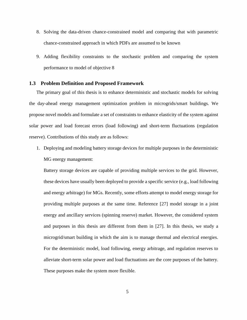
Figure 1 summarizes the proposed energy management and the tasks performed in this
thesis.
8
Deterministic Model Stochastic Model
With
Flexibility
Constraints
Without
Flexibility
Constraints
Parametric
Chance-
Constrained
Data-Driven
Chance-
Constrained
Set
Confidence
Level
Update
Confidence
Level
Start
Solving the
Optimization
Problem
Inputs
End
Figure 1. Proposed framework.

9
CHAPTER 2. LITERATURE REVIEW
Microgrids
Technically, MGs were existed in 1882. The first MG was built by Thomas Edison, and it was
named the Manhattan Pearl Street Station. Since there was no centralized grid on those years, this
station can be called as the first MG in the world history [29]. Definition of a microgrid is a single
governable object regarding the grid containing a set of loads and DERs including renewable
energy resources surrounded by clearly defined electrical boundaries that are controlled by the
microgrid operator. MGs are small-sized power grids that operate at low voltage level. A microgrid
can be operated in both grid-connected mode or islanded mode. This feature allows MG to connect
and disconnect from the distribution feeder [30]. Under normal circumstances, MGs are connected
to medium voltage grids, and it is possible that they can exchange power with the distribution
feeder [31]. Operating in the islanded mode is useful when there is a blackout (or its possibility)
because the MG operator can disconnect the local grid from the main grid. As depicted in Figure
2, a microgrid may contain various devices, e.g., photovoltaic (PV) cells, wind turbines, batteries,
and portable gas generators as DERs, lights, office equipment components, fans, air conditioning
(AC) units, white goods, and heaters [32].
There are many advantages expected with utilizing MGs. Economic and environmental
benefits are the primary purposes of MGs. Including renewable energies into the energy
management decreases the overall MG operation cost. Moreover, the amount of carbon emission
to nature will be decreased by employing renewable energy resources. Growing the renewable
energy production would allow us to replace carbon-concentrated energy sources and remarkably
lessen harmful gas emissions. For example, National Renewable Energy Laboratory discovered

10
that if 80% of the U.S. electricity production comes from renewable sources by 2050, global
warming emissions from electricity generation will be reduced by nearly 81% [33].
PV Cells
Wind Turbines
Air Conditioning
CHP
White Goods and
Office Equipments
Energy Storage
Fan
Lights
Substation
Hot Water
Thermal Loads
Smart Building
(microgrid)
Distribution Feeder
Multi-Carrier
Thermal
Electricity
Figure 2. An example of microgrid system.
MGs have different types depending on the role of usage. The first type is campus
environment microgrids. They are onsite-generation with multiple controllable loads. This MG
type is also called as a community microgrid. The second type is remote MGs. These MGs are
always in an islanded mode and connect to the main grid. They are usually located in rural that
which are far from transmission and distribution lines. The third type is military based MGs whose
objective is both physical protection and cyber security for military facilities to ensure reliable

11
power without the distribution feeder. The fourth type is commercial and industrial MGs. The main
reason for this type of MGs is power supply safety and consistency. For example, any electrical
interruption to industrial factories, which triggered by the distribution feeder, may cause huge
revenue losses [32].
Many research projects are going on microgrid planning, control, and operation. In [34], an
MG planning approach is proposed for unclear situations with specifying investment of DERs and
an operation subproblem to define cost functions. A robust optimization technique is used to solve
and examine the planning problem. Reference [35] shows that provisional MGs do not have the
islanding function of microgrids, but they are reliant on coupled microgrids for islanding
capability. By using a robust optimization approach, physical and economic uncertainties in MG
planning are managed. The objective function is to minimize investment cost. Che et al. suggest
that MGs should be interconnected to the distribution feeder for many reasons [36]. Consequently,
determining optimal planning for community MGs with volatile renewable energies is applied by
the minimum cut-set methodology to improve reliability and minimize the operation cost of multi
microgrids. Clustering analysis is used to describe characteristics of wind and solar energy in MGs.
Reference [37] proposed a theoretical framework to show how a cooperative planning of
renewable generations in interconnected MGs is more efficient than an uncooperative planning.
The primary objective is cost sharing among several areas that are suitable to establish wind farm
and solar panels such that all MGs will get benefit from this planning method. In [38], a new
approach is presented to reconfigure an islanded microgrid with aiming to minimize fuel
consumption and switching, and to maximize system loadability.

12
Load Management
Energy management represents the concept of optimizing energy systems. Although there is a
great deal of experience referring to optimizing generation and distribution aspects of energy, the
demand side management is one of the most attractions for the researcher. Load management is a
part of demand-side management (DSM), also known as a demand-side response (DSR) that can
be defined as demand-side measures to improve system performance at the consumer level. The
next generation of the smart grid technology accompanied by DSM technologies will offer an
opportunity of making smarter decisions for customers regarding the quantity and time energy
consumption. This capability of management and usage control is referred as DSM. In fact, DSM
is a set of adjustable and interconnected programs that provide customers with the chance of
playing a more significant role in time shifting of their electricity demand during peak periods and
minimizing their overall costs [39]. Load management is a crucial function for decreasing peak
load. Managing loads to make the power system more efficient can be done in different ways. The
load shapes of daily or seasonal electricity demands between peak and off-peak times can be
described by six techniques [40-42], which are illustrated in Figure 3. Peak clipping and valley
filling work on reducing the peak and valley level respect to increase the security of smart grids.
Load shifting is to move loads in time to low load demand intervals during periods of peak
demands. Shifting demands is a solution if loads are adjustable with shifting behavior. Controllable
load management not only has the advantage of peak shaving, frequency control, or voltage
regulation but also is beneficial for balancing service for a period of energy usage [43]. Examples
of controllable loads are ovens, fridges, washing machine and dryer, air conditioners, and water
heating. Therefore, these types of loads are called controllable or shiftable loads. Strategic
conservation is a technique that works toward optimization of load shape achievement using
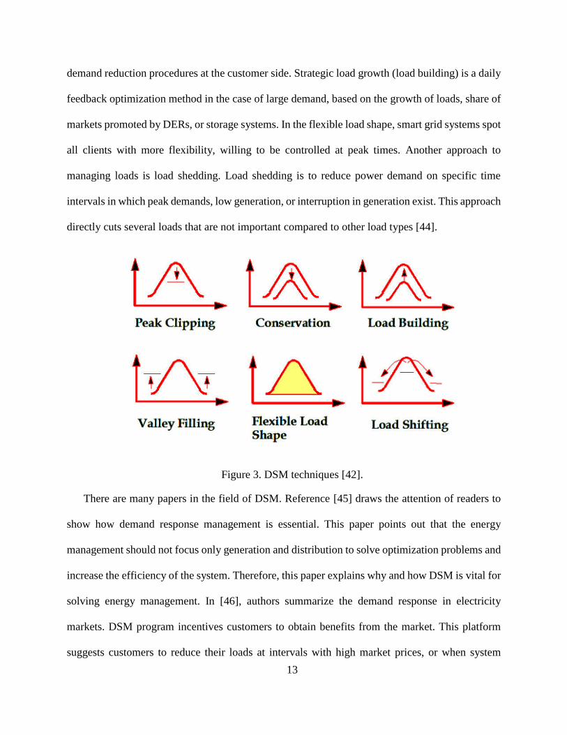
13
demand reduction procedures at the customer side. Strategic load growth (load building) is a daily
feedback optimization method in the case of large demand, based on the growth of loads, share of
markets promoted by DERs, or storage systems. In the flexible load shape, smart grid systems spot
all clients with more flexibility, willing to be controlled at peak times. Another approach to
managing loads is load shedding. Load shedding is to reduce power demand on specific time
intervals in which peak demands, low generation, or interruption in generation exist. This approach
directly cuts several loads that are not important compared to other load types [44].
Figure 3. DSM techniques [42].
There are many papers in the field of DSM. Reference [45] draws the attention of readers to
show how demand response management is essential. This paper points out that the energy
management should not focus only generation and distribution to solve optimization problems and
increase the efficiency of the system. Therefore, this paper explains why and how DSM is vital for
solving energy management. In [46], authors summarize the demand response in electricity
markets. DSM program incentives customers to obtain benefits from the market. This platform
suggests customers to reduce their loads at intervals with high market prices, or when system
14
reliability is at risk. According to this paper, DSM can diminish electricity prices and meanwhile
improve the system reliability. Reference [47] proposes a demand response approach centered on
the utility maximization in households. These households operate different appliances with
specific benefits depending on the model, or the size of their power consumption. Every household
solves its optimization problem selfishly aiming at maximizing its revenue. This paper claims that
a utility company can use a dynamic pricing scheme to assess the price and benefit all system.
Sivaneasan et al. put forward a protective demand response management (DRM) for commercial
buildings using the building energy management system (BEMS) to guarantee that the scheduled
or estimated demand limit is not transcended while minimizing the total cost of energy usage in
buildings [7]. This DRM uses two important demand response techniques; namely, dynamic
electric vehicle (EV) charge scheduling to ensure that EV charging is not exceeding limits of
demand, and load shedding based on the importance of loads.
Energy Management
Energy management is a structured and methodical coordination of procurement, distribution,
operation, and planning of energy to meet requirements at some given energy balance value or
equivalence [48]. This systematic organization is simply built upon power generation and load
demand equality. Depending on the energy system, there might be an issue when generation is
higher than load or vice versa. To overcome these kinds of problems, energy management aims to
make energy generation and consumption balanced, which means generation minus load equals to
zero.
Many researchers have conducted studies on energy management in buildings and microgrids.
Implementation of a deterministic energy management method and operational planning for
business customers in MGs with PV-based active generator are presented in [12]. Two players are

15
considered in this management problem; namely, customer-side energy management and base
energy management for MG. These two players exchange information between each other and
solve the planning and management problem according to the prediction for PV production and
load forecasting. Reference [49] proposes a home energy management algorithm for managing
energy in household appliances. This paper intents control and manage appliances to have total
consumption of households below an indicated demand limit. However, it may decrease the
customers’ comfort level. Wang et al. assert an energy management design for common places in
buildings by keeping the temperature on the current value, decreasing or increasing by one degree
[50]. This approach offers to obtain the same net payoff among all occupants and incentivize the
system by using the Arrow-d’Aspremont-Gerard-Varet (AGV) mechanism. Reference [51]
recommends an approximate dynamic programming with temporal difference learning for PV
thermal and battery systems. This approach can be extended to large systems like adding multiple
controllable devices without increasing the computational costs when compared to the classical
dynamic programming and stochastic mixed-integer programming. The approximate dynamic
programming differs from the classical dynamic programming since its approximations make the
problem less complex. A study in [13] offers an energy management method for residential
buildings using solar energy as a thermal and electrical generating unit. The objective is to
minimize total costs of households while aiming to maximize users’ comfort. This problem is
solved by the two-stage stochastic programming. Rastegar et al. introduce a two-level framework
for energy management in residential buildings [52]. In the first level, each customer runs its
optimization problem and sends the appliances’ operation data to an aggregator. In the second
stage, a multi-objective optimization problem with a fuzzy decision-making procedure is solved
to minimize the system load curve and costs without any additional cost to customers. Reference
16
[53] suggests minimizing the energy consumption costs by setting the air conditioning system of
a meeting room in a commercial building according to a time gap, attendee numbers, room size,
and the air conditioning system. A mixed-integer programming (MIP) is formulated and solved by
a heuristic algorithm to find a near-optimal solution. Reference [54] merges a machine learning
based on neural network method, optimization, and data structure design for DRM considering
controllable, uncontrollable, and regulatable loads in a building. The objective is to minimize the
total cost of energy consumption. The neural network is trained to follow the energy consumption
of heating ventilation and air conditioning. Reference [55] proposes a new concept of energy
management for buildings connecting to MG. This system includes DC and AC subsystems that
are connected via a DC/AC converter. Thus, this system provides active and reactive power to the
grid as an ancillary service. The building is a dispatchable load or generator depending on the
power flow direction. Reference [14] presents a multi-stage mixed integer stochastic programming
to minimize the operating costs of buildings. An energy hub system is presented that consists of
the grid power, solar power, combined heat and power (CHP) with boiler units, and energy storage
to supply electricity and heat to consumers. The study of [15] offers an approach to manage energy
in smart buildings integrated with the smart grid. Multiple buildings create a cluster and exchange
their excess energy with each other to maximize their revenue. This optimization problem is a
game theory in which and buildings’ managers are players aiming at optimizing their revenue.
Multi-Carrier Energy Systems
Multi-carrier energy systems, also known as energy hubs, are systems including multiple forms
of energies, such as electrical, thermal, and cooling [6]. These energies may be converted and
stored in the hub. An energy hub is demonstrated in Figure 5, in which CHP’s input is natural gas,
but we can get outputs as electrical and thermal energy.

17
Wind
Sun
Grid (i.e.,
distribution
feeder)
Natural
Gas
Wind
Turbines
PV Cells
CHP with
Boiler Unit
Energy
Storage
Electrical
Loads
Thermal
Loads
Energy HubInput
Output
Gas
Electrical
Renewable
Thermal
Figure 5. Multi-carrier energy system.
Many studies have conducted on multi-carrier energy systems since [6] has been published by
Geidl et al. Reference [56] proposes a multi-objective optimization of energy hubs and demand
predictions to minimize operation costs and CO2 emission. An adaptive neuro-fuzzy inference
system combined with genetic algorithm is deployed to solve the problem. The problem is solved
in multi-steps; load prediction, energy hub’s constraints construction, and optimizing. In [57],
Najafi et al. present a bi-level stochastic programming for an energy hub. Hub managers maximize
their profit at the upper level, while clients minimize their costs at the lower level. The original
problem, which is nonlinear, is transformed into a linear form using the Karush–Kuhn–Tucker
(KKT) conditions and strong duality condition. Meanwhile, clients and hub managers may sell
heat and electricity to the pool. Reference [58] introduces a generalized analytical approach to

18
assess the reliability of renewable energy hub system covering both heat and electricity. This study
models EVs and wind turbines. EVs transfer energy to the energy hub and the distribution feeder.
Centralized and decentralized management algorithms are presented that yield different reliability
indices. In [59], a comprehensive approach is developed with integrating the energy supply side
including solar energy, main grid, and batteries and the demand side (buildings).
Power Reserve
In power systems, the operating reserve is the backup generation that is available to balance
power generation and load in case of occurrence of an unpredicted event [60]. The regulation
reserve is the subterm for the operating reserve. Hence, this type of reserve is available by
increasing output power of generators that are already connected to the grid. The regulation reserve
is shown in Figure 6. However, we cannot say that all reserve types are ready for use immediately.
In MGs, microturbines, diesel generators, and batteries can be the source of regulation reserves.
Because of the fast ramping-capability, battery storage devices are suitable for the regulation
reserve procurement.
Due to the growth of renewable energies, assessing reserve capacity is important to minimize
operation costs and maximize system reliability. In [61], to quantify the amount of reserve,
uncertainty analysis of PV generator and load is performed. Reference [62] proposes an approach
to compensate uncertainties, which are occurred by wind power, by scheduling the operating
reserve of thermal generators. The operating reserve is defined as an ancillary service. The
objective is to minimize the operation cost. which consists of costs of the fuel consumed by thermal
units and reserve. As discussed in [63], the operating reserve is critical because of the impact of
wind variability and uncertainty. This paper categorizes effects of wind uncertainties and identifies
different reserve types, namely, non-event and event reserves.
19
Load
and
Res
erve
Po
wer
(kW
)
Generation
Time
Generation
Load
Reserve
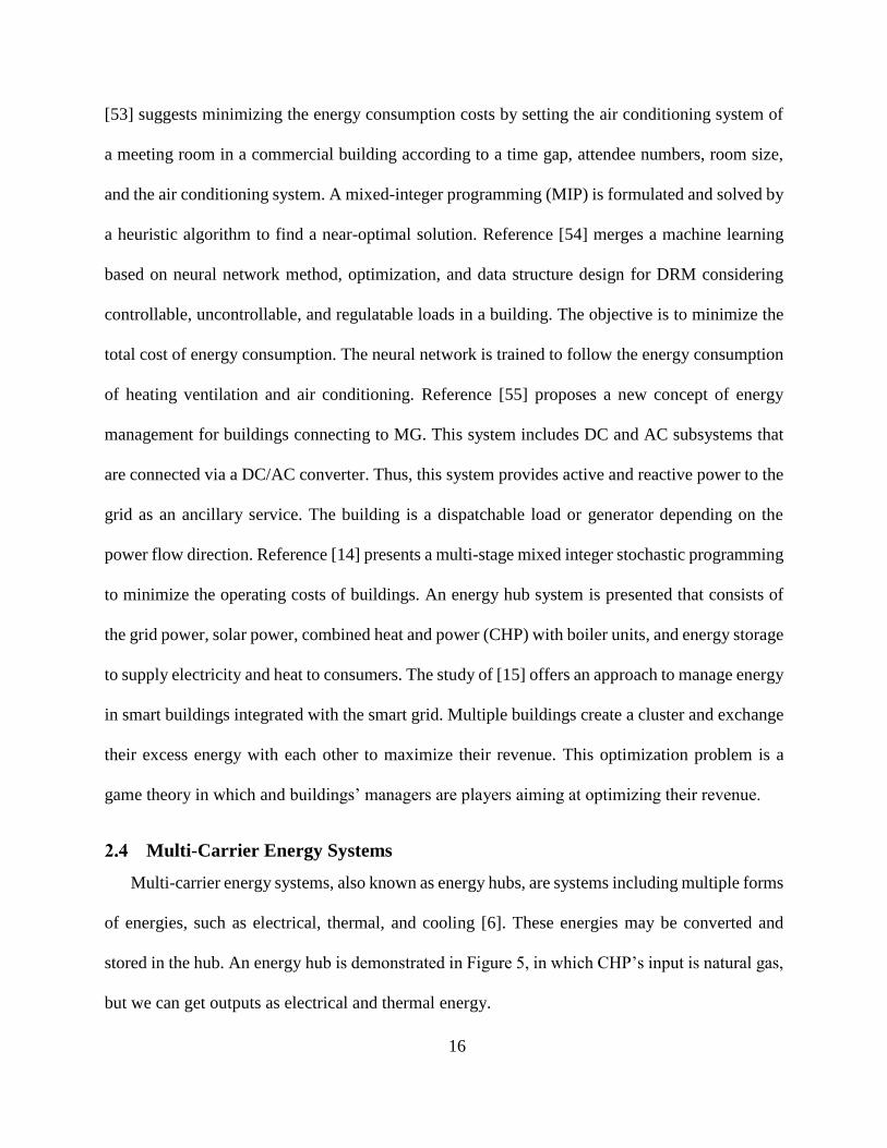
Figure 6. Regulation reserve.
Distributed Energy Resources (DERs)
Distributed energy resources (DERs) refer to small-scale generating units that are deployed to
produce power at the distribution voltage level [64]. DERs are usually installed close to load
centers. Various types of DERs exist, such as microturbines, combustion turbines, fuel cells, CHPs,
energy storage systems (ESSs), PV systems, and wind turbines. Some of the main benefits of DERs
include reducing frequency variations, having the backup energy after power outages, peak
shaving when demand is high, and producing low-cost energy. In following sub-sections, PV
systems, ESSs, and CHPs will be explained briefly.
PV Systems
PV cells can be installed almost everywhere, i.e., on the ground, rooftops, urban areas, and
even oceans. Solar energy is a free and clean energy. The main benefits of PV cells are inexpensive

20
maintenance, long life components, no carbon emissions, no noise, and high reliability. However,
PV cells have some including low solar panel area and power rates, not suited for backup energy
without battery, and variable power outputs [65].
Solar power uncertainty and variability bring new challenges into energy management
problems. Many studies have addressed this issue. Solar generation needs to be predicted for
energy management purposes. Reference [66] discusses that non-parametric probabilistic
predicting methods are more efficient for solar generation modeling. The probability and
cumulative density functions of solar power are forecasted for every 10-minute time interval. This
non-parametric method is based on extreme learning machine as a quick model for creating density
functions of an uncertain data set given in 1-minute resolutions. Benefits of using yearly solar
radiation data sets as an alternative of using PDFs to model solar power is discussed in [67].
Stochastic models are involved in many papers to model uncertainties of solar energy in system
scheduling problems [68-70].
Energy Storage Systems
Energy storage systems have seen tremendous attention in power systems community since
they play a critical role in renewable energy integration. ESSs are required to move toward a more
sustainable energy infrastructure. A battery storage device stores energy to use whenever it is
needed. This technology is deployed in the home energy management, electricity grid, and
transportation systems.
Many papers and books have been published in the field of energy storage systems planning
and operation. Since battery installation costs are high, determining the size of batteries is crucial.
Reference [71] presents a solution for optimal sizing of energy storage systems considering hourly
and intra-hourly time intervals. Similarly, reference [72] proposes a method to optimize the energy

21
storage size according to the magnitude of load demand in a microgrid. This paper also gives a
method to find the optimal location.
Batteries have fast-ramping capabilities that are very useful for the grid. Because of this
feature, load following and regulation reserve services can be provided by a battery [73]. The
regulation reserve is needed to alleviate the impact of short-term fluctuations in a power system.
The amount of regulation reserve is determined with respect to generation (e.g., renewable energy)
and load fluctuations. In [71], energy storage is deployed for load following and regulation reserve
procurement. The load following is to balance generation and load in 5-minute interval basis, and
the regulation reserve is considered to damp possible 1-minute renewable generation and load
fluctuations. In [74], Jintanasombat et al. propose a battery ramping method that compensates or
reduces the power fluctuations that is occurred from PV system. The battery’s ramping rate is fixed
at a reasonable value to decrease oscillations.
CHP Systems
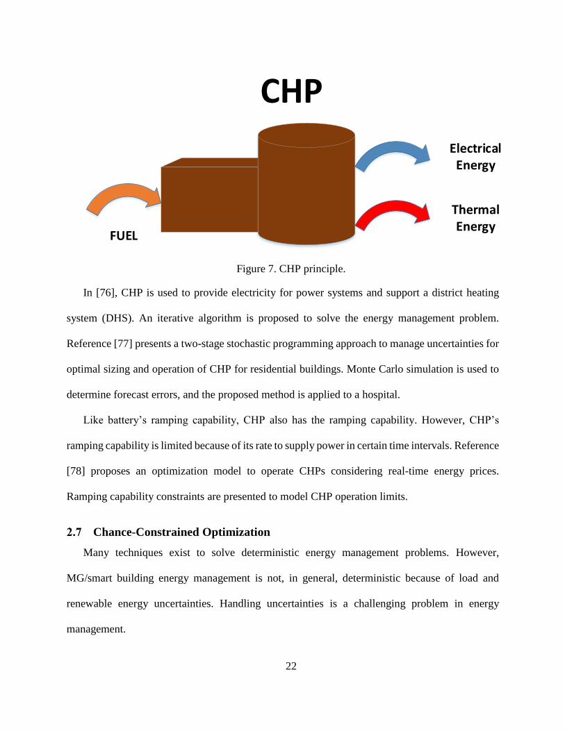
Combined heat and power (CHP) is the integration of thermal and electrical energy production.
The CHP principle is illustrated in Figure 7. According to other DERs, CHP is more efficient
because of its capability of supplying thermal and electrical energies. A typical CHP might have
an efficiency of 90%., which is divided into 40% for electrical energy and 60% for thermal energy
generation. MicroCHP (small-scale CHP) units are widely employed in smart buildings [75].
22
FUEL
Thermal Energy
Electrical Energy
CHP
Figure 7. CHP principle.
In [76], CHP is used to provide electricity for power systems and support a district heating
system (DHS). An iterative algorithm is proposed to solve the energy management problem.
Reference [77] presents a two-stage stochastic programming approach to manage uncertainties for
optimal sizing and operation of CHP for residential buildings. Monte Carlo simulation is used to
determine forecast errors, and the proposed method is applied to a hospital.
Like battery’s ramping capability, CHP also has the ramping capability. However, CHP’s
ramping capability is limited because of its rate to supply power in certain time intervals. Reference
[78] proposes an optimization model to operate CHPs considering real-time energy prices.
Ramping capability constraints are presented to model CHP operation limits.
Chance-Constrained Optimization
Many techniques exist to solve deterministic energy management problems. However,
MG/smart building energy management is not, in general, deterministic because of load and
renewable energy uncertainties. Handling uncertainties is a challenging problem in energy
management.

23
Several optimization techniques have been proposed in the literature to unravel this challenge.
Robust optimization [79], stochastic programming [80], approximate dynamic programming [81],
and chance-constrained programming [19] are among the most popular techniques for handling
uncertainties. Chance-constrained (CC) programming is of the most suitable techniques for short-
term microgrid energy management. This technique was first introduced by Charnes and Cooper
in 1959 to solve optimization problems with uncertainties [19]. Chance-constrained programming
is an optimization method which allows system operators or customers to stipulate a confidence
level (𝛼) or, inversely, risk level (1 − 𝛼) of fulfilling probabilistic constraints [82]. The general
concept of chance constraints is that probability of a constraint must be equal to or larger than a
fixed confidence level. Chance constraints might be in the form of individual or joint chance
constraints. In individual CCs (ICCs), a set of probabilistic constraints are formulated each of
which has its own confidence level. On the contrary, a confidence level is defined for joint CCs
(JCCs) in which the probability of satisfaction of all constraint together mush be equal to larger
than the defined confidence level.
Chance constraints (or probabilistic constraints) can be categorized into two classes: classical
constraints in which PDFs of random variables are known and data-driven CCs in which PDFs of
random variables are unknown.
The Classical-Chance-Constrained (CCC) Optimization
The CCC model can also be called the parametric chance-constrained programming. In CCC,
PDFs of uncertain or random variables are known, and follows certain PDF types such as normal,
Beta, Poisson, Lognormal, and Binomial. To solve CCCs, they can be converted to their equivalent
deterministic models with respect to PDFs and confidence levels [83]. When converting the CCC

24
model to the deterministic programming, the random variable will be equal to the expected value
of random variable plus Z-quantile multiplied by the standard deviation of the random variable,
i.e., �̃� = 𝐸(𝑥) + 𝑍(𝑥) ∗ 𝜎(𝑥). For example, quantile of 95% confidence level for normal PDF is
fixed and 1.96 [84]. Therefore, the considered optimization problem, with converted CCCs, is
solved with standards solvers.
There are many papers dealing with power system management with the parametric CC model
(or CCC). Reference [85] proposes the stochastic optimization scheduling model for 31-bus and
118-bus IEEE system considering loads and wind energy as random variables. An ICC model is
applied to handle uncertainties. Reserve requirements and line flows are designed as CCs.
Similarly, reference [11] uses the CCC model to manage random variables in power system
planning. This paper proposes a planning approach for energy storage sizing considering hourly
and intra-hour scheduling intervals. Wind generation and load demand are taken into account as
uncertainties. In [86], Liu et al. solve the energy management problem in MGs considering
uncertainties. They use CCC to handle variabilities occurring from the load and renewable
energies. CCCs are converted into their deterministic models by taking inverse cumulative
distribution function (CDF) of random variables.
Data-Driven Chance-Constraints (DDCCs)
Unlike CCCs, PDFs of random variables are unknown in data-driven chance constraints. A
DDCC is also called a non-parametric chance constraint. A central aspect of the DDCC model [87,
88] is defining a new confidence set or reduced risk level to handles uncertainties with unknow2n
PDFs in an optimization problem. Historical data of random variables, which might not follow any
known PDF types, are used to estimate PDFs. The confidence level (risk level) of probabilistic
constraints are adjusted according to estimation errors. In [82], Bruno et al. reformulate the DDCC

25
programming with the right-hand side uncertainty to a set of algebraic constraints. Finding the
pointwise forecasted errors using kernel smoothing to estimate PDF is the key point of this paper
to rearrange chance constraints. This study (which is the core of our energy management approach
in Chapter IV) proposes the following steps to reformulate DDCC:
1. Estimate unknown PDFs of ransom variables
2. Choose the best divergence function [87] and find pointwise errors
3. Calculate a divergence tolerance 𝑑 with the chosen function
4. Determine a new confidence level (1 − 𝛼′) or a reduced risk level 𝛼′
5. Solve the optimization problem with an updated confidence level.
Therefore, a new confidence level will be calculated through these steps by taking inverse CDF
(quantile function) of a random variable. Steps 1 to 4 are performed offline. After finding quantile
of the random variable, it will be put in the problem and the considered optimization is solved.
A non-parametric CC optimization is presented in [89] to plan and operate battery units in
power distribution grids. Authors imply that they do not impose any assumptions on finding PDFs
of active power flows in lines and voltages at buses. Numerical studies show that the non-
parametric CC model is more efficient than the parametric one. Reference [90] uses the DDCC
model to deal with nowcasting and forecasting PV power production based on real data of multi-
generation microgrids. Reference [91] proposes a data-driven risk-averse chance-constrained unit
commitment model to handle uncertainties of renewable energy generation in system scheduling.
Risk aversion roots come from the probability distribution of wind generation, and it is assumed
that wind power production has the worst-case probability.

26
CHAPTER 3. DETERMINISTIC MICROGRID ENERGY MANAGEMENT
In this chapter, a deterministic optimization model is presented for microgrid energy
management. Forecasted values of load and renewable generation are used for scheduling
purposes. That is, it is assumed that load and generation sources are deterministic. Without loss of
generality, we use solar power generation as the renewable energy source (note that the proposed
model is general and can be deployed for any types of renewable generation, e.g., wind generation).
The operation horizon is considered to be 24 hours. Since in an MG the load may vary minutes to
minutes, each hour is divided into 12 equal intervals, each interval is 5 minutes, and the forecasted
load and sola data of every 5-minute are used. This makes the scheduling more accurate since 5-
minute time resolution forecast values are, usually, more accurate than hourly values.
Another important feature of the proposed model is its capability to deploy energy storage
systems for multiple purposes. Storage not only participates in 5-minute load following but also
provides ramping capability for the system. The ramping capability can be interpreted as the grid
flexibility in response to short-term (i.e., 1-minute) fluctuations. As battery storage is a fast device,
it provides adequate flexibility for the MG to alleviate the impact of short-term load and generation
fluctuations. Thus, the proposed model allows storage to provide multiple services to the grid
(energy and ancillary services), and thus it provides more incentive for a private sector to invest in
storage and makes a profit out of this asset (which is expensive). The deterministic energy
management model consists of continuous and integer variables. Thus, the formulated
optimization problem is a Mixed-Integer Linear Programming (MILP). The objective function is
to minimize the total operation costs. The optimization includes storage energy and ramping
constraints, restrictions of energy transaction between the microgrid and distribution feeder,
27
constraints of CHP with boiler unit and its ramp rate, controllable loads, and thermal and electrical
energy balances.
In the proposed formulation, we model electricity and thermal loads. The objective is to
manage two forms of energy taking into account dependencies between thermal and electrical
generations and demands. Combined Heat and power (CHP) with boiler units can participate in
both electricity and thermal power generation.
Assumption: We consider no uncertainties in the deterministic MG energy management
presented in this chapter. Solar power generation and load are set to their forecast values (expected
values) based on 5-minutes time intervals. We assume that short-term fluctuations, which need to
be compensated by the system ramping capabilities (flexibility constraints), the worst possible
short-term fluctuation values are 20% of the 5-minute forecasted values. Short-term fluctuations
should be damped in a 1-minute time interval basis. That is, 1-minute ramping capabilities are
required.
Equipment/devices: The considered microgrid consists of PV panels, combined heat and
power with a boiler unit, battery storage, controllable thermal loads, controllable electrical loads,
non-controllable thermal loads, and non-controllable electrical loads.
Notations: We denote a vector with a bold non-italic font (e.g., 𝐗). Parameters are denoted by
non-bold non-italic font (e.g., Cfg,t). Variables are determined by non-bold italic font (e.g., 𝑃𝑔𝑡,𝑡).
E(⋅) refers to the expected value. Random variables are indicated by (⋅̃) (e.g., P̃sol,t).

28
Objective Function
The objective of the MG is to minimize its costs. These costs are a summation of costs of
buying energy from the distribution feeder, operation costs of CHP with the boiler (fuel cost),
operation costs of energy storage. Note that solar generation has no operation cost. In addition, the
operation cost of storage, which is related to maintenance costs, is a small value that depends on
the charging/discharging power. A microgrid may receive revenue for selling energy to the
distribution feeder. Thus, the objective function of the optimization problem is the summation of
costs minus the revenue as follows:
min𝐗
∑(Cfg,t ∗ 𝑃𝑓𝑔,𝑡 − Ctg,t ∗ 𝑃𝑡𝑔,𝑡 + Cgas,t ∗ (𝐹𝑐ℎ𝑝,𝑡 + 𝐹𝑏𝑜𝑖,𝑡) + Cb ∗ 𝑃𝑏𝑐,𝑡 + Cb ∗ 𝑃𝑏𝑑,𝑡)
𝑇
𝑡=1
(1)
𝐗 ∈ {𝑃𝑓𝑔,𝑡 , 𝑃𝑡𝑔,𝑡, 𝑃𝑐ℎ𝑝,𝑡, 𝑃𝑣𝑔,𝑡, 𝑃𝑏𝑐,𝑡, 𝑃𝑏𝑑,𝑡, 𝐹𝑐ℎ𝑝,𝑡, 𝐹𝑏𝑜𝑖,𝑡,
𝐻𝑏𝑜𝑖,𝑡, 𝑆𝑡, 𝐻𝑐ℎ𝑝,𝑡, 𝐼𝑒 , 𝐼ℎ, 𝐼𝑓𝑔,𝑡, 𝐼𝑡𝑔,𝑡, 𝐼𝑐ℎ𝑝,𝑡, 𝐼𝑐𝑛𝑒,𝑡, 𝐼𝑐𝑛ℎ,𝑡}
where 𝐗 is the set of continuous and integer variables. 𝑃𝑓𝑔,𝑡, 𝑃𝑡𝑔,𝑡, 𝑃𝑐ℎ𝑝,𝑡, 𝐹𝑏𝑜𝑖,𝑡, 𝑃𝑏𝑐,𝑡, 𝑃𝑏𝑑,𝑡, 𝑃𝑏𝑐,𝑡,
𝑃𝑏𝑑,𝑡, 𝑃𝑣𝑔,𝑡, 𝐻𝑏𝑜𝑖,𝑡, 𝐻𝑐ℎ𝑝,𝑡, 𝐹𝑐ℎ𝑝,𝑡, 𝑆𝑡, 𝐼𝑒, and 𝐼ℎ are continuous variables, while 𝐼𝑓𝑔,𝑡, 𝐼𝑡𝑔,𝑡, 𝐼𝑐ℎ𝑝,𝑡,
𝐼𝑐𝑛𝑒,𝑡, and 𝐼𝑐𝑛ℎ,𝑡 are integer variables. The total cost is minimized over the considered operation
horizon 𝑇. The costs of power selling to the distribution feeder (Ctg,t), purchasing from the
distribution feeder (Cfg,t ), fuel usage by CHP with boiler (Cgas,t), battery charging (Cbc), and
battery discharging (Cbd) are inputs of the optimization problem.
To ensure feasibility of the solution, constraints of each equipment and the system constraints
must be satisfied. The constraints are formulated in the following section. Note that two types of
constraints are formulated. The first type is the constraints that must be satisfied for every time
29
interval t (such as energy balance). The second type is the intertemporal constraints that
interconnect the intervals (such as the ramping capability of the generating units).
Battery Storage Constraints
The battery is charged or discharged under different circumstances. For example, the battery
might inject power to the grid during peak-load hours, while it might store energy during off-peak
hours and when the solar generation is high. Batter storage has energy and power constraints as
formulated below:
𝑆𝑡 = Si + (ηbc. 𝑃𝑏𝑐,𝑡 −𝑃𝑏𝑑,𝑡
ηbd) ∗ Δt t = 1 (2)
𝑆𝑡+1 = 𝑆𝑡 + (ηbc. 𝑃𝑏𝑐,𝑡+1 −𝑃𝑏𝑑,𝑡+1
ηbd) ∗ Δt t > 1 (3)
Smin ≤ 𝑆𝑡 ≤ Smax ∀𝑡 (4)
Si = Sf (5)
0 ≤ 𝑃𝑏𝑐,𝑡 ≤ Pbcmax ∀𝑡 (6)
0 ≤ 𝑃𝑏𝑑,𝑡 ≤ Pbdmax ∀𝑡 (7)
Constraint (2) shows the battery status at t = 1 when Si is constant at t = 0. Parameter Δt is
the time resolution (i.e., intra-hour time interval) that is considered to be 5-minute in this thesis.
Constraint (3) models the energy storage status at time intervals t > 1. This constraint connects
state of energy of storage at time interval t to time interval t − 1. Energy stored in the battery
depends on the charging/discharging power. Constraint (4) presents maximum and minimum
30
limits of battery energy status. The initial and final energy status of battery should be the same as
modeled in (5). This constraint keeps the energy level at a certain level to ensure that the battery
is prepared for the next day. Constraints (6) and (7) specify maximum charging and discharging
power limits.
A battery should be charged or discharged more than a certain level. That is, the depth of state
of charging and discharging (DSOC) needs to be restricted as model in (8).
|ηbc. 𝑃𝑏𝑐,𝑡 −𝑃𝑏𝑑,𝑡
ηbd| ≤ DSOC ∀t (8)
Regulation Reserve (Flexibility) Constraints
Microgrid must have adequate flexibility to alleviate short-term (i.e., 1-minute) load and
generation fluctuations. This is a critical issue in the presence of non-dispatchable renewable
energy sources. Thus, we propose to model the system ramping capabilities in the MG energy
management model. We formulated constraints (9)-(12) to ensure that the system has adequate
ramping capability to respond to short-term load and solar generation fluctuations. Since the
battery has a fast-ramping capability, we deploy this device to provide adequate ramping (i.e., an
ancillary service) for MG. This ramping is defined as MG’s regulation reserve.
𝑃𝑏𝑑,𝑡𝑟𝑟 ≥ ϖ ∗ P𝑠𝑜𝑙,𝑡 + ω ∗ 𝑃𝑛𝑐,𝑡 ∀t (9)
𝑃𝑏𝑑,𝑡𝑟𝑟 = Pbd
max − 𝑃𝑏𝑑,𝑡 ∀t (10)
𝑃𝑏𝑐,𝑡𝑟𝑟 ≥ ϖ ∗ P𝑠𝑜𝑙,𝑡 + ω ∗ 𝑃𝑛𝑐,𝑡 ∀t (11)
𝑃𝑏𝑐,𝑡𝑟𝑟 = Pbc
max − 𝑃𝑏𝑐,𝑡 ∀t (12)

31
where ϖ and ω determine the required regulation reserve. Parameter ϖ (ω) determines percentage
of possible solar generation (load) fluctuations compared to its forecasted value for each interval
𝑡. These parameters are considered as constants that are determine based on the operator’s
experience and historical information. Constraint (9) indicates that the total regulation reserve
capability for discharging battery must be equal or greater than ϖ% of solar power, and ω % of
non-controllable electrical loads. In this thesis, ϖ and ω are considered to be 10 or 20% and 2.5
or 5%, respectively. The extra ramping capability of the battery (i.e., battery power rating), which
is equal to the maximum charging/discharging rate minus charging/discharging rate at interval t,
determines the MG’s regulation reserves. Constraint (10) imposes the ramping up (power injected
to the system by battery) requirements. Similarly, constraints (11) and (12) model the ramping
down (power injected to battery from the system) requirements. These four constraints guarantee
that MG has enough flexibility and regulation reserves to alleviate the impact of short-term solar
and load fluctuations.
Modeling a Virtual Generation Source by Combining Battery and Solar Generation
One of the main tasks of storage is to capture the solar generation variations. We proposed to
merge storage charging/discharging power and solar generation to build a virtual generation
source. The output power of this virtual source, at interval t, is denoted as 𝑃𝑣𝑔,𝑡. The goal is to
keep 𝑃𝑣𝑔,𝑡 as smooth as possible so that a small amount of generation variations is observed at the
grid level. Constraints of the virtual generation source are as follows:
𝑃𝑣𝑔,𝑡 = E(P̃sol,t) + (𝑃𝑏𝑑,𝑡/ηbd) − (𝑃𝑏𝑐,𝑡 ∗ ηbc) ∀t (13)

32
0 ≤ 𝑃𝑣𝑔,𝑡 ≤ Pvg,tmax ∀t (14)
𝑃𝑣𝑔,𝑡−1 − Pbrd ≤ 𝑃𝑣𝑔,𝑡 ≤ 𝑃𝑣𝑔,𝑡−1 + Pbru t > 1 (15)
Pvg,tmax = E(P̃sol,t
max) +Pbd
max
ηbd (16)
Constraint (13) models the virtual source power output (𝑃𝑣𝑖𝑟𝑡𝑢𝑎𝑙,𝑡). E(�̃�𝑠𝑜𝑙,𝑡) denotes the
expected solar generation. Constraint (14) shows limits of the virtual source power output.
Depending on possible solar power fluctuations, ramping up and down rates are assessed by the
system operator with aiming at smoothness of the virtual generation. Constraint (15) is formulated
to eliminate forecast errors of PV cells. Constraint (16) defines the maximum of virtual power
generation, which equals to expected solar power (mean value) plus the maximum battery
discharging. By deploying ramping up and down of battery, we can handle forecast errors and
obtain a smoother power output than the solar generation. Therefore, solar smoothness will be
obtained by activating these constraints. Note that the ramp rates 𝑃𝑏𝑟𝑑 and 𝑃𝑏𝑟𝑢 are determined by
the system operator’s experience and system condition (historical data can be utilized for this
purpose).
Constraints of Electricity Transaction with Distribution Feeder
The microgrid exchange energy with the distribution feeder. This power exchange is
bidirectional, from the distribution feeder to MG or vice versa. To model this power exchange,
four decision variables are introduced; namely, power injected from MG to the distribution feeder
(𝑃𝑡𝑔,𝑡), electricity supplied from the distribution feeder to MG (𝑃𝑓𝑔,𝑡), and two binary variables
indicating the direction of power flow (𝐼𝑓𝑔,𝑡 and 𝐼𝑡𝑔,𝑡).
33
0 ≤ 𝑃𝑓𝑔,𝑡 ≤ M𝑔𝑓 ∗ 𝐼𝑓𝑔,𝑡 ∀t (17)
0 ≤ 𝑃𝑡𝑔,𝑡 ≤ Mgt ∗ 𝐼𝑡𝑔,𝑡 ∀t (18)
𝐼𝑓𝑔,𝑡 + 𝐼𝑡𝑔,𝑡 ≤ 1 ∀t (19)
𝐼𝑓𝑔,𝑡 ∈ {0,1}
𝐼𝑡𝑔,𝑡 ∈ {0,1}
Constraints (17) and (18) impose upper and lower bounds of power exchange. Constraint (19)
determines the status of selling to and buying from the distribution feeder. Buying and selling
cannot happen at the same time since we assume a coupling point between the distribution feeder
and MG. variables 𝐼𝑓𝑔,𝑡 and 𝐼𝑡𝑔,𝑡 are binary. Thus, (19) does not allow them to be 1 at the same
time. Note that these two variables might be zero at the same time that mean MG does not exchange
energy with the distribution feeder.
Constraints of CHP and Boiler Unit
CHP has two important roles in microgrid energy management: electricity generation and heat
production. High usage of CHP during winter seasons fulfills both electricity and thermal power
demand since PV panels are not able to obtain solar radiation efficiently comparing to the summer
[92]. Two sets of binary variables (𝐼𝑐ℎ𝑝,𝑡, 𝐼𝑏𝑜𝑖,𝑡) are introduced to determine the CHP and boiler
ON/OFF status at interval 𝑡. In addition, electrical power generated by CHP (𝑃𝑐ℎ𝑝,𝑡) and thermal
power production by CHP and the boiler (𝐻𝑐ℎ𝑝,𝑡 , 𝐻𝑏𝑜𝑖,𝑡) are decision variables. Constraints of
CHP with a boiler unit are formulated as follows:
𝐹𝑐ℎ𝑝,𝑡 = a. 𝑃𝑐ℎ𝑝,𝑡 + b. 𝐼𝑐ℎ𝑝,𝑡 ∀t (20)

34
𝐻𝑐ℎ𝑝,𝑡 = ηhr(𝐹𝑐ℎ𝑝,𝑡 − 𝑃𝑐ℎ𝑝,𝑡) ∀t (21)
Pchpmin. 𝐼𝑐ℎ𝑝,𝑡 ≤ 𝑃𝑐ℎ𝑝,𝑡 ≤ Pchp
max. 𝐼𝑐ℎ𝑝,𝑡 ∀t (22)
𝐻𝑏𝑜𝑖,𝑡 = ηboi. 𝐹𝑏𝑜𝑖,𝑡 ∀t (23)
Hboimin. 𝐼𝑏𝑜𝑖,𝑡 ≤ 𝐻𝑏𝑜𝑖,𝑡 ≤ Hboi
max. 𝐼𝑏𝑜𝑖,𝑡 ∀t (24)
where 𝐹𝑐ℎ𝑝,𝑡 and 𝐹𝑏𝑜𝑖,𝑡 are fuel power consumed by CHP and the boiler, respectively. Constraint
(20) indicates that when CHP is ON, it consumes the minimum 𝑏 amount of natural gas without
power generation. For power generation, 𝑎 amount of natural gas is used to produce electricity.
Constraint (21) models the connection between CHP’s thermal and electrical energy productions.
The minimum and maximum power generation limits are imposed in (22). Constraint (23)
specifies conversion of the boiler’s fuel power consumption to the thermal power. The minimum
and maximum thermal energy generation limits of the boiler are imposed by (24).
While battery has the fast ramping capability to compensate solar power fluctuations, CHP has
ramping ability to follow non-controllable loads in the system (note that the fast ramping capability
is useful for short-term fluctuations (1-minute basis) while CHP ramping is more useful for load
following (5-minute basis) purposes). Whether the load is increasing or decreasing over time, CHP
can ramp up/down its power to eliminate load variations. Limits of ramping up and down rates of
CHP are modeled by (25) to follow non-controllable loads in 5-minute time resolution. Similar to
(25), constraint (26) is formulated for CHP’s thermal power ramp rates.
𝑃𝑐ℎ𝑝,𝑡−1 − Pchp,rd ≤ 𝑃𝑐ℎ𝑝,𝑡 ≤ 𝑃𝑐ℎ𝑝,𝑡−1 + Pchp,ru t = 2, … , T (25)
𝐻𝑐ℎ𝑝,𝑡−1 − Hchp,rd ≤ 𝐻𝑐ℎ𝑝,𝑡 ≤ 𝐻𝑐ℎ𝑝,𝑡−1 + Hchp,ru t = 2, … , T (26)
35
Constraints of Controllable Loads
Two sets of thermal and electrical loads are considered: controllable and non-controllable.
While non-controllable loads are constant in each interval 𝑡 without proving any flexibility for the
operator to control them, controllable loads provide the flexibility for the operator to defer them
from interval an interval to another interval. Controllable loads are assumed as non-interruptible
and deferrable loads. When an appliance is ON, it should be ON for 𝑀𝑖𝑛𝑜𝑛𝑒 time intervals without
any interruption. Decision variable 𝑃𝑐𝑛,𝑡 is the amount of electricity consumed by controllable load
in interval 𝑡, and binary variable 𝐼𝑐𝑛𝑒,𝑡 determine the status of the controllable electrical load in
interval 𝑡. Constraint for controllable loads are as follows:
Pcn,tmin. 𝐼𝑐𝑛𝑒,𝑡 ≤ ∑ 𝑃𝑐𝑛𝑡
T
t=1
∀t (27)
Minone = T𝑒on ∗ Interval Number (28)
𝐼𝑒 = 𝐼𝑐𝑛𝑒,𝑡 − 𝐼𝑐𝑛𝑒,𝑡−1 t = 2, … , T (29)
RNG𝑒 = t: min(T, t + Minone − 1) t = 2, … , T (30)
𝐼𝑐𝑛𝑒,𝑅𝑁𝐺𝑒≥ 𝐼𝑒 (31)
∑ 𝐼𝑐𝑛𝑒,𝑡
T
t=1
= Minone (32)
where RNG stands for the range of controllable load intervals. Constraint (27) represents the
minimum limits of the controllable electrical loads when they are switched ON. Constraint (28)
shows the minimum ON time when an appliance is switched ON. For example, if the controllable
load’s minimum ON hour is 3 hours, and our system is divided into 12 intervals, the minimum ON
36
time for this controllable load is 36 intervals. Expression (29) states that the constraints of a
controllable load are redundant unless indicator 𝐼𝑒 is 1. Constraint (30) indicates Minone time
interval cannot exceed its limit, and a controllable load does not continue on the next day.
Constraint (31) ensures that the indicator is 1 when Minone is active in the range of time. As state
in (32), the summation of binary variables must be equal to Minone time intervals to stop after the
time of Minone.
A similar concept, as controllable electrical loads, is valid for controllable thermal loads.
Hcn,tmin. 𝐼𝑐𝑛ℎ,𝑡 ≤ ∑ 𝐻𝑐𝑛𝑡
T
𝑡=1
∀ 𝑡 (33)
Minonh = Thon ∗ Interval Number (34)
𝐼ℎ = 𝐼𝑐𝑛ℎ,𝑡 − 𝐼𝑐𝑛ℎ,𝑡−1 t = 2, … , T (35)
RNGℎ = t: min(T, t + Minonh − 1) t = 2, … , T (36)
𝐼𝑐𝑛ℎ,𝑅𝑁𝐺ℎ≥ 𝐼ℎ (37)
∑ 𝐼𝑐𝑛ℎ
T
𝑡=1
= Minonh (38)
where Hcn,tmin is the minimum thermal power produced by CHP.
Energy Balance Constraints
Power generation must meet the demand at each interval 𝑡. We assume that solar power (Psol,t)
and non-controllable electrical and thermal loads (Pnc,t, Hnc,t), at each interval, are known
(forecast values) as inputs of the energy management problem. Hence, the following electricity

37
and thermal power balance constraints are formulated using the expected values of the load and
solar generation:
𝑃𝑓𝑔,𝑡 − 𝑃𝑡𝑔,𝑡 + 𝑃𝑐ℎ𝑝,𝑡 + 𝑃𝑏𝑑,𝑡 − 𝑃𝑏𝑐,𝑡 + E(P̃sol,t) = E(P̃nc,t) + 𝑃𝑐𝑛,𝑡 ∀t (39)
ηhc(𝐻𝑐ℎ𝑝,𝑡 + 𝐻𝑏𝑜𝑖,𝑡) = E(H̃nc,t) + 𝐻𝑐𝑛,𝑡 ∀t (40)
Constraint (39) states that the supply of electrical power (left-side of the power balance
equation) must be equal to the demand (right-side of the power balance equation). Similar to (34),
constraint (40) ensures that the heat production is equal to the thermal load.
Case Studies and Results
The proposed scheduling method is applied to manage thermal and electrical energy in a
community microgrid. The lower and upper bounds of the power generated by CHP are 0 and 12
kW. Parameters 𝑎 and 𝑏 of CHP are set to 1.41 and 8.7, respectively. CHP’s and boiler’s thermal
coil efficiency are 0.93; and thermal recovery efficiency of CHP and efficiency of the boiler are
0.72 and 0.9, respectively. The minimum and maximum energy limits of the battery storage are 5
and 50kWh. The initial (and final) state of charge is 20kWh. Charging and discharging power
limits of the battery are 4.8kWh. The prices of buying energy from the distribution feeder at
different hours is as follows:
12: 00 𝑎𝑚 ~ 9: 00 𝑎𝑚 → 0.051$/𝑘𝑊ℎ
9: 00 𝑎𝑚 ~ 3: 00 𝑝𝑚 → 0.119$/𝑘𝑊ℎ
3: 00 𝑝𝑚 ~ 7: 00 𝑝𝑚 → 0.071$/𝑘𝑊ℎ
7: 00 𝑝𝑚 ~ 11: 00 𝑝𝑚 → 0.119$/𝑘𝑊ℎ
11: 00 𝑝𝑚 ~ 12: 00 𝑎𝑚 → 0.051$/𝑘𝑊ℎ
38
The price of selling energy to the distribution feeder is $0.067/kWh over the considered
operation horizon. The natural gas price is $0.031/kWh for every time interval. Note that all prices
are converted into $/kW-5mins, and energy units are also changed from kWh to kW-5mins.
We study two cases to show the effectiveness of the proposed scheduling method.
• Case 1: Deterministic optimization without flexibility (regulation reserve) constraints
• Case 2: Deterministic optimization with flexibility (regulation reserve) constraints
All simulations are carried out using YALMIP toolbox in Matlab [93] and ILOG CPLEX
12.4’s MILP solver on a 3.7 GHz personal computer with 16GB RAM.
Case 1: Deterministic Optimization without Ramping Constraints
The deterministic model is solved neglecting the flexibility constraints. In other words,
constraints (9) – (16), (25), and (26) which ensure having adequate regulation reserve and ramping
capability, are disregarded. This the classical deterministic model presented in the literature. The
optimization problem is solved. The MG operation cost is $18.76.
Figure 8 shows the state of charge (percentage) of the battery storage over 24 hours. The battery
charging and discharging power is depicted in Figure 9. The battery stays in an idle mode (i.e., no
charging and discharging activities) from 12:00 am until 5:00 am. From 5:00 am to 7:00 am, the
battery becomes charged. From 7:00 am to 1:30 pm, power consumption and generation go up
while the amount of energy in the battery remains stable. Then, the battery injects power to MG
because of the high power demand. It is observable from Figure 9 that battery discharges a large
amount of power around 1:45 pm, and then it reduces the discharging power to meet at 40% energy
level at the end of the day (battery must meet 40% of state of the charge at the end of the day to
have the same energy as beginning of the day).

39
Figure 8. Battery energy status in percentage over the considered operation horizon.
Figure 9. Battery charging and discharging powers over the considered operation horizon.
Figure 10 illustrates the power exchanged between MG and the distribution feeder over the
considered operation horizon. While selling and buying power from/to the distribution feeder
cannot occur at the same time, they can be inactive at the same time. For instance, from 8:00 pm
to 10:00 pm, MG and the distribution feeder exchange no power, i.e., 𝑃𝑓𝑔 = 𝑃𝑡𝑔 = 0.

40
Figure 10. Power bought/sold from/to the grid over the considered operation horizon.
The controllable electrical and thermal loads are scheduled as shown in Figure 11. The
controllable electrical load must be ON for 3 hours, and the controllable thermal load must be ON
for 4 hours. Therefore, according to power generation and loads in MG, controllable loads are
shifted into specific time intervals to optimize the objective function.

41
Figure 11. Controllable electrical and thermal controllable loads' ON-OFF times over the
considered operation horizon.
Figure 12 shows all electrical loads and power generations in one graph. CHP is ON in many
time intervals as the gas price is not high. The amount of power sold to the distribution feeder is
large especially, during the daytime when PV panels are producing power a large amount of power.
Conversely, in most time intervals during the daytime, importing energy from the distribution
feeder is zero. The amount of power purchased from the distribution feeder is the largest when the
controllable loads are ON.

42
Figure 12. Electrical power generation and loads over the considered operation horizon.
The thermal power consumption and generation are represented in Figure 13. Since CHP is
often ON, it supplies thermal power in many time intervals. If there is lack of thermal generation,
to balance load and generation, the boiler unit of CHP becomes involved to compensate the thermal
power deficits.
In this case, the battery is used for 5-minute load following purposes. However, the battery is
an expensive device, and using such an expensive device only for load following may not be
economically justifiable. Thus, it may discourage a user to install battery only for one service.

43
Figure 13. Thermal power generation and loads over the considered operation horizon.
Case 2: Deterministic Optimization with the Ramping Constraints
In this case, we deploy battery not only for load following purposes but also for regulation
reserve procurement. The flexibility constraints of battery and CHP are added to the deterministic
model. Other than including ramping capabilities of CHP and energy storage, everything else
remains the same as in Case 1. The total operation cost is $ 19.25. Because of modeling of the
regulation reserve requirements, the operation cost of Case 2 is larger than that in Case 1. Although
the operation cost is larger, battery and CHP provide adequate regulation reserves for MG. This
enhances the flexibility of the system to respond to short-term solar generation and load
fluctuations. The flexibility constraints make the system more secure and reliable. Thus, this $0.46
(19.25-18.76) cost increment can be interpreted as security costs.

44
Figure 14 and 15 demonstrate the regulation reserve capacity of the battery (ramp up/down)
over 24-hour horizon. MG’s requirements for ramping short-term fluctuations are shown with solid
red line. In several intervals (for instance, 155-170th and 218th intervals in Figure 14, and 64-67th
and 79-85th intervals in Figure 15), the regulation reserve is not adequate to compensate short-term
fluctuations. Therefore, Case 1 has no enough ramping up/down capabilities to fulfill the possible
short-term solar and load fluctuations in these intervals. On the contrary, Case 2 always has
sufficient regulation reserve to respond to prospective short-term fluctuations and keep the system
safe and reliable.
Figure 16 demonstrates the battery energy status (percentage) over the 24-hour horizon. In
contrast to Figure 8, energy status is not smooth. The charging and discharging powers are shown
in Figure 17. The battery does not become charged/discharged from 12:00 am to 6:45 am. After
6:45 am, the battery is active until 8:00 pm. Specifically, the battery is charged from 6:45 am to
8:30 am because of the extra power generation in MG. After 4:45 pm, the energy storage injects
power to MG since load is large, and solar generation is zero after 8:00 pm. The battery energy
level at the end of the day is the same as that at the beginning of the day (i.e., 40%).
Figure 18 shows power exchanged with the distribution feeder over 24 hours. From 12:00 am
to 5:00 am, MG sells energy produced by CHP to the distribution feeder to obtain revenue when
MG’s load is low. Since the controllable electrical load is scheduled to be ON from 6:00 am to
9:00 am (see Figure 19), buying power from the distribution feeder becomes active. A similar
buying/selling pattern as in Case 1 is observed from 9:00 am to 12:00 am.

45
Figure 14. Regulation reserve (ramping up) over the considered operation horizon.
Figure 15. Regulation reserve (ramping down) over the considered operation horizon.

46
Figure 16. Battery energy status in percentage with ramping over the considered operation
horizon.
Figure 17. Battery charging and discharging powers with ramping over the considered
operation horizon.

47
Figure 18. Power buying from the grid and selling to the grid with ramping over the
considered operation horizon.
Figure 19. Controllable electrical and thermal loads' ON-OFF times with ramping over the
considered operation horizon.

48
Figure 20 displays the power output of the virtual generation and solar over the considered
operation horizon. The solid blue line represents the virtual output power, and the dash-dot brown
line shows the solar power. While the solar power is not smooth, the virtual output power is
smooth. This smoothness is obtained by deploying ramping capabilities of the battery and
constructing an imaginary power source by connecting the battery and solar power. This
smoothness is desirable for MG as it enhances the system performance and power quality.
Figure 20. Output of virtual power generation and solar power comparison with ramping over
the considered operation horizon.
Figure 21 illustrates all electrical loads and power productions over the 24-hour operation
horizon. CHP is ON in all intervals since the gas price is not high and CHP supports both electrical
and thermal loads. During the hours of daylight, while PV panels produce energy, power selling
(buying) to (from) the distribution feeder is mostly existing (zero) and continuous. Contrariwise,

49
power buying from the distribution feeder has its peak amount when the controllable electrical
load is ON. The thermal energy productions and demand is represented in Figure 22. The thermal
loads are supported mostly supported by CHP. In several hours in which demand is larger than
CHP’s capacity, the boiler provides thermal power to balance the generation and demand.
Figure 21. All electrical power generation and loads with ramping over the considered
operation horizon.

50
Figure 22. All thermal power generation and loads with ramping over the considered
operation horizon.

51
CHAPTER 4. PROBABILISTIC SYSTEM SCHEDULING WITH CHANCE
CONSTRAINTS
Stochastic behavior of solar generation and load was neglected in the deterministic microgrid
energy management presented in Chapter 3. These two random variables were modeled by their
expected (forecast) values. However, ignoring uncertainties might increase risk level of the system.
In addition, the obtained results might not be far from the optimal solution after the true realization
of random variables. Thus, a deterministic model might not be realistic for microgrid energy
management since solar generation and load uncertainties play an important role in power
generation and load balance constraints.
In this chapter, we propose a chance-constrained optimization to account for solar generation
and load uncertainties in microgrid energy management. Probability distribution functions (PDFs)
of the random variables are needed to formulate chance constraints. Although several know classes
of PDF (e.g., normal PDF) are used in the literature to model solar generation and load, distribution
functions of these random variables may not always follow known PDFs. Indeed, PDFs depends
on types of the load and location of solar panels. Thus, distribution functions may not belong to
any class of know PDFs. In addition, if PDFs are not estimated accurate enough, chance constraints
may fail to provide accurate and efficient results. This increases the system risk level and degrades
quality of the obtained results. We propose to formulate a set of data-driven chance constraints to
model solar generation and load uncertainties. The proposed method is non-parametric that
imposes no assumption on the type of distribution functions. That is, PDFs of solar generation and
load are not forced to belong to known classes of probability distributions. These PDFs belong to
unknown classes of probability distributions. We deploy adaptive kernel density estimator to
estimate PDFs of solar generation and load. We modified the confidence level (or risk level) of
the chance constraints according to errors of the estimated PDFs. Our proposed determine the
52
optimal MG operation point while accounting for the estimation errors of non-parametric PDFs.
This approach is more realistic compared to the parametric chance-contained approach and can be
deployed by MG operators regardless of their geographical locations as long as the operators have
historical data of random variables (i.e., solar generation and load).
Note that in this chapter, we do not repeat all constraints formulated in Chapter 3 since most
of the will stay unchanged even after considering solar generation and load uncertainties. We only
focus on constraints that will change after considering uncertainties (i.e., constraints that include
at least of the random variables P̃sol,t, P̃nc,t, and H̃nc,t ).
Data-Driven Chance-Constrained Solution Methodology
Solar generation and load uncertainties can be modeled in MG energy management using
different techniques, such as scenario generation, robust optimization, chance-constrained
optimization, etc. Scenario-based techniques are computationally expensive, and robust
optimization provides the most conservative solution. However, because of the nature of our
problem, the MG operator may prefer a technique that is not too conservative and computationally
expensive. Thus, we focus on the chance-constrained optimization as it is efficient and easy to
implement for the MG operator. The main drawback of the chance-constrained optimization is its
sensitivity to the choice of PDF for modeling random variables. If the PDFs do not accurately
model the behavior of the random variable, the chance-constrained programming may fail to
provide accurate and reliable results.
To address this shortfall, a data-driven non-parametric chance-constrained method is presented
for day-ahead MG scheduling. We deploy adaptive kernel density estimation to estimate PDFs of
solar generation and load using historical data.

53
Consider the following probabilistic chance constraint:
infP∈D
ℙ{A𝐗 + b ≤ 𝜉�̃�} ≥ 1 − 𝛼 ∀j (41)
where ℙ{⋅} denote the probability measure, and 𝜉�̃� is a random variable. Expression (41)
indicates that the probability of constraint A𝐗 + b ≤ 𝜉�̃� is satisfied must be larger than or equal
1 − 𝛼. Parameter 𝛼 is the risk level. This is an individual chance constraint (ICC). ICC refers to a
situation in which the probability of satisfying a constraint is larger than a confidence level. If a
set of constraint exist inside ℙ{⋅} (i.e., ∀j is inside ℙ{⋅}) , it means that the probability of satisfying
all constraints together must be larger than or equal to a confidence level [82]. In this thesis, we
work on ICC because of the nature of the considered MG energy management problem.
The risk level 𝛼 is set by the operator according to the system condition and requirements. In
the classical parametric chance-constrained optimization, since PDF of the random variable is
known, (41) always satisfies the desirable confidence level (risk level). However, since PDFs of
solar generation and load are not exactly the same the forecasted ones (obtained by a forecaster),
constraint (41) does not guarantee the required confidence level.
To account for prediction errors and the fact that probability distributions of solar generation
and load might not belong to any class of known PDFs, we convert the risk level α to a reduced
risk level α′. That is, we increase the confidence level (1 − α) to (1 − α′) where 1 − α ≤ 1 − α′.
The more accurate the predictions are (i.e., less prediction error), the closer α′ is to α. to avoid
having a negative risk level (which might happen if prediction errors are large), the risk level is
modified as 𝛼+′ = max{0, 𝛼′} [82]. The new risk level is replaced in (41) to express a non-

54
parametric chance constraint taking into account the prediction errors and the accuracy of PDFs.
We also replace ℙ{⋅} by ℙ̂{⋅} since a known PDF is replaced by an unknown one.
ℙ̂{A𝐗 + b ≤ 𝜉�̃�} ≥ 1 − 𝛼+′ ∀j (42)
where ℙ̂ is the estimated distribution function and 𝛼+′ = max{0, 𝛼′}. We adopt kernel density
estimator to model PDFs of solar generation and load, and then formulate data-driven chance
constraints (DDCC). Finding the pointwise forecasting errors using kernel smoothing is the critical
point to rearrange constraints. The amount of error affects 𝛼+′ , and consequently the constraints.
Reformulated DDCC model is performed by following steps [82]:
1. Estimate the unknown PDF
2. Choose the best divergence function and find the pointwise errors [82, 87]
3. Calculate the divergence tolerance 𝑑 with the chosen function
4. Update the increased confidence level (1 − 𝛼′) or the reduced risk level (𝛼′)
5. Solve the optimization problem with the new confidence level
We elaborate Steps 1 to 4. In the first, PDFs of random variables (i.e., solar power and load) is
done using some adaptive kernel density estimator. Then, based on the histogram and PDF of
historical data, we calculate the pointwise errors by subtracting Y-axis of histogram from the
estimated PDF. These errors create a new PDF. Taking quantile of this PDF at the given confidence
level provides us with the divergence tolerance 𝑑. When we have 𝑑, one of the three divergence
functions (Kullback-Leibler, Variation Distance, and X Divergence of Order 2 [87]) can be used
to calculate the reduced risk level (𝛼′).

55
Steps 1 to 4 are performed offline, and their outputs are PDFs and 𝛼′. Then, 𝛼+′ quantile of the
random variable are calculated by taking inverse cumulative distribution function (CDF) of the
random variable. Finally, the optimization problem is solved in Step 5. This procedure is explained
in detailed as follows.
Most of the deterministic constraints presented in Chapter 3 (i.e., (2) - (8) and (10) - (33)) will
stay the same (i.e., deterministic) in the probabilistic MG energy management. The objective
function of the probabilistic model is the same as (1). Only the constraints that include random
variables, i.e., solar generation (P̃sol,t), non-controllable electrical loads (P̃nc,t), and non-
controllable thermal loads (H̃nc,t), need to be converted into chance constraints. Note that in the
deterministic model, the expected (forecasted) values of the random variables were used.
The virtual generation source constraint (13), in which the solar power is a random variable, is
replaced by the following inequality chance constraint:
ℙ̂(𝑃𝑣𝑔,𝑡 − (𝑃𝑏𝑑,𝑡/ηbd) + (𝑃𝑏𝑐,𝑡 ∗ ηbc) ≥ P̃sol,t) ≥ 1 − αE ∀t (43)
Similarly, the power balance constraint (39) is rewritten as follows:
ℙ̂(𝑃𝑓𝑔,𝑡 + 𝑃𝑐ℎ𝑝,𝑡 + 𝑃𝑏𝑑,𝑡 + P̃sol,t ≥ 𝑃𝑡𝑔,𝑡 + 𝑃𝑏𝑐,𝑡 + P̃nc,t + 𝑃𝑐𝑛,𝑡) ≥ 1 − α𝐸 ∀t (44)
Let us introduce a new variable as 𝑃𝐵𝑎𝑙𝑎𝑛𝑐𝑒,𝑡 = 𝑃𝑓𝑔,𝑡 + 𝑃𝑐ℎ𝑝,𝑡 + 𝑃𝑏𝑑,𝑡 − 𝑃𝑡𝑔,𝑡 − 𝑃𝑏𝑐,𝑡 − 𝑃𝑐𝑛,𝑡.
Then, the chance constraint (44) is reformulated as follows:
𝑃𝐵𝑎𝑙𝑎𝑛𝑐𝑒,𝑡 = 𝑃𝑓𝑔,𝑡 + 𝑃𝑐ℎ𝑝,𝑡 + 𝑃𝑏𝑑,𝑡 − 𝑃𝑡𝑔,𝑡 − 𝑃𝑏𝑐,𝑡 − 𝑃𝑐𝑛,𝑡 (45)

56
ℙ̂(𝑃𝐵𝑎𝑙𝑎𝑛𝑐𝑒,𝑡 ≥ P̃nc,t − P̃sol,t) ≥ 1 − αE ∀i, ∀t (46)
Statistically, two random variables can be in the same constraint only if both PDF types are
the same (e.g., normal PDF). Otherwise, two random variables cannot be in the same constraint.
Since in our study, PDF types of solar power and load are the unknown, we need to reformulate
(46). We introduce a dummy decision variable for solar power generation (i.e., Sol𝑡) and rewrite
(46) as follows:
ℙ̂(𝑆𝑜𝑙𝑡 ≥ P̃sol,t) ≥ 1 − α𝐸 (47)
ℙ̂(𝑃𝐵𝑎𝑙𝑎𝑛𝑐𝑒,𝑡 ≥ P̃nc,t − 𝑆𝑜𝑙𝑡) ≥ 1 − αE ∀i, ∀t (48)
The left-hand side of (47) and (48) includes decision variables, and the right-hand side contains
the random variables. Thus, constraint (44) is replaced by (45), (47), and (48).
The thermal power balance constraint (40) is converted into the probabilistic constraint (49)
since the non-controllable thermal load is a random variable. The acceptable risk levels of thermal
and electrical energies might not be the same. Thus, we define α𝐸 the risk level of the electrical
power balance and 𝛼𝐻 as the risk level of the thermal power balance. These risk levels imply the
probability of the chance constraints satisfaction (i.e., success).
ℙ̂(ηhc(𝐻𝑐ℎ𝑝,𝑡 + 𝐻𝑏𝑜𝑖,𝑡) − 𝐻𝑐𝑛𝑡𝑟,𝑡 ≥ H̃nc,t) ≥ 1 − αH ∀t (49)
57
Deterministic Model of DDCC
The probabilistic chance constraints are not in the closed form to be handled by standard
solvers. We convert these constraints to their equivalent deterministic format by calculating 𝛼
quantile (i.e., inverse CDF ) of the estimated PDFs.
Consider the following probabilistic chance constraint:
ℙ̂{𝑔𝑗(𝑥) ≥ 𝜉�̃�} ≥ 1 − 𝛼𝑗,+′ ; ∀j (50)
Constraint (50) is detailed as the probability of 𝑔𝑗(𝑥) to be greater than or equal to the random
variable 𝜉�̃� must be at least 1 − 𝛼𝑗,+′ . in other words, the estimated CDF of the random variable
calculated at 𝑔𝑗(𝑥) must be at least 1 − 𝛼𝑗,+′ . Constraint (50) is defined as the following constraint:
�̂�𝜉�̃�(𝑔𝑗(𝑥)) ≥ 1 − 𝛼𝑗,+
′ ; ∀j (51)
where �̂�𝜉�̃�(. ) is the estimated CDF of the random variable 𝜉�̃�. Inequality (50) can be written with
the inverse CDF (quantile function):
𝑔j(𝑥) ≥ �̂�𝜉�̃�
−1(1 − 𝛼𝑗,+′ ) ; ∀j (52)
where �̂�𝜉�̃�
−1(. ) is the estimated quantile function. Notice that the estimated quantile function is a
constant value determined by performing several steps. Consequently, the right-hand side of (52)
becomes a fixed value, and the left-hand side remains unchanged. Using this concept, we can

58
convert chance constraints (43), (47), (48), and (49) into their solvable equivalent deterministic
model, which are linear constraints.
𝑃𝑣𝑔,𝑡 − (𝑃𝑏𝑑,𝑡/ηbd) + (𝑃𝑏𝑐,𝑡 ∗ ηbc) ≥ 𝑆𝑜𝑙𝑡 ∀t (53)
𝑆𝑜𝑙𝑡 ≥ F̂�̃�𝑠𝑜𝑙,𝑡
−1 (1 − αE) ∀t (54)
𝑃𝐵𝑎𝑙𝑎𝑛𝑐𝑒,𝑡 ≥ F̂�̃�𝑛𝑐,𝑡
−1 (1 − αE) − 𝑆𝑜𝑙𝑡 ∀t (55)
(ηhc(𝐻𝑐ℎ𝑝,𝑡 + 𝐻𝑏𝑜𝑖,𝑡) − 𝐻𝑐𝑛,𝑡 ≥ F̂�̃�𝑛𝑐,𝑡
−1 (1 − αH) ∀t (56)
Constraints (53) - (56) are in a form (i.e., linear inequality constraints) that can be handled by
standard solvers.
Case Studies and Results
The data-driven chance-constrained (DDCC) model is applied to a community microgrid. The
input data is the same as the data used in Chapter 3, except for solar generation, non-controllable
electric load, and non-controllable thermal load that is random variables. The considered operation
horizon is 24 hours. Each hour is divided into 12 intervals (i.e., each intra-hour time interval = 5-
minute). All simulations are carried out using the YALMIP toolbox in Matlab and ILOG CPLEX
12.4’s MILP solver on a 3.7 GHz personal computer with 16GB RAM.
We study three cases to show the effectiveness of the proposed algorithm:
• Case 1: the parametric chance-constrained optimization without the flexibility constraints
• Case 2: the non-parametric chance-constrained optimization without the flexibility
constraints
• Case 3: the non-parametric chance-constrained optimization with the flexibility constraints.
59
Case 1: Parametric Chance-Constrained Optimization without Flexibility
Constraints
We consider that uncertain variables have known PDFs. The forecasted 5-minute solar
generation, thermal load, and electricity demand follow normal PDF. Thus, the classical
parametric chance-constrained optimization is formulated to minimize the operation cost taking
into account the electrical and thermal constraints. The short-term fluctuations of solar generation
and load are neglected, and hence, the flexibility constraints, i.e., ramping capabilities of energy
storage and CHP, are ignored. That is, constraints (9) – (16), (25), (26), (39) - (40), and (53) are
disregarded. Thus, storage is used for the energy arbitrage and load following purposes. The
confidence level of the chance constraints is set to 95%. The total operation costs of MG is $24.08.
Figure 23 shows the state of charge of the battery over the considered operation horizon. Battery
is charged when solar generation is high, while it is discharged during the peak load hours. The
battery state of charge at the end of the day is equal to that at 𝑡 = 0. Figure 24 demonstrates battery
charging and discharging powers. The battery becomes charged from 2:30 am to 8:00 am (when
the energy price is low), and it becomes discharged from 8:00 am to 12:00 am (when the energy
price is high). The discharging power is more frequent after 7:00 pm when energy price is high
and solar generation is zero.
The power purchased/sold from/to the distribution feeder illustrated in Figure 25. From 12:00
am to 4:30 am, the demand is low, and MG sells its excess energy to the distribution feeder. When
the power consumption increases from 5:00 am to 2:00 pm, MG buys energy from the distribution
feeder. During the remaining hours, selling and buying attitudes change depending on the power
generation and load.
60
Figure 23. State of charge of battery in percentage over the considered operation horizon.
Figure 24. Battery charging and discharging powers over the considered operation horizon.

61
Figure 25. The power buying from and selling to the distribution feeder over the considered
operation horizon.
Controllable electrical and thermal loads schedule are depicted in Figure 26. When the
electrical (thermal) load becomes ON, it must stay ON for 3 (4) hours. Therefore, these controllable
loads are shifted according to the demand, power generation, and energy price. The controllable
electrical load is ON from 5:00 am to 8:00 am. On the other hand, the controllable thermal load
becomes ON from 10:00 am to 2:00 pm. Shifting controllable loads helps the operator to minimize
the total operation costs.
Figure 27 shows all electricity generations and demands in one diagram over the 24-hour
horizon. CHP is ON most of the times since the gas price is low. Selling power is active during
the night time (when CHP is ON) and when solar generation is high. Conversely, the power buying
from the distribution feeder is usually inactive when PV panels gather solar radiation. On the other
hand, imported power from the distribution feeder has its highest amount when the controllable
electrical load is ON.

62
Figure 26. Controllable electrical and thermal loads' ON-OFF times over the considered
operation horizon.
Figure 27. All electrical power generation and loads over the considered operation horizon.
The thermal power generations and loads are depicted in Figure 28. According to the thermal
energy balance, the thermal generation must be equal to or higher than the thermal load. Since

63
CHP produces thermal power when generating electricity, the thermal power generation is larger
than load in several intervals (i.e., thermal power produced by CHP is wasted). If enough thermal
power is not provided by CHP, the boiler unit is activated to fulfill the power deficit.
Figure 28. All thermal power generation and loads over the considered operation horizon.
Case 2: Data-Driven Chance-Constrained Optimization without Flexibility
Constraints
In this case, we assume that a data set (i.e., sample points) exists for each random variable. For
the sake of comparison, we generate sample points from normal PDFs given in Case 1. By doing
so, we can compare the results of the proposed algorithm with those obtained by the parametric
chance-constrained optimization. Although we know that the sample points follow normal PDFs,
we impose no assumption on the sample points while estimating a PDF of each random variable.
That is, sample point might or might not belong to any classes of known PDFs. The short-term
fluctuations of solar generation and load are neglected, and hence, the flexibility constraints, i.e.,
the ramping capabilities of energy storage and CHP, are ignored. That is, constraints (9) – (16),

64
(25), (26), (39) - (40), and (53) are disregarded. The proposed DDCC optimization is applied. We
study three scenarios. In scenario 1, 50 samples exist for each random variable at each time
interval, and in scenarios 2 and 3, we have 100 and 200 samples for each random variable at each
time interval, respectively. To estimate PDFs from the sample points, we have tested various the
non-parametric estimation methods, such as the Adaptive Kernel Density Estimation (AKDE), the
Diffusion KDE [94], and Matlab KDE. We have selected the AKDE since its accuracy was higher
than other methods.
The DDCC approach aims at finding a new confidence level according to the forecasting errors
generated from solar power, electrical load, and thermal load. The updated confidence level
guarantees that the old confidence level is achieved even with forecast errors. That is, the new
confidence level guarantees the system reliability level defined by the operator; however, the
operation cost might increase compared to the old confidence level (i.e., parametric approach).
We set the risk level α=0.1 (i.e., the confidence level is 90%). According to the AKDE
estimation error, the adjusted risk level for scenario 1 is 𝛼𝑠1+ = 0.081. The adjusted risk level of
50 samples load random variable at 200th interval guarantees that the system is secure with a
confidence level of 90% even if AKDE’s estimation is not accurate, and the true realizations of
the solar generation and load do not lie on the estimated PDFs. The adjusted risk levels for
scenarios 2 and 3 are 𝛼𝑠2+ = 0.085 and 𝛼𝑠3
+ = 0.086, where s2 and s3 are scenarios with 100 and
200 samples, respectively. The adjusted risk level becomes closer to the exact risk level as the
number of sample points increases (𝛼 − 𝛼𝑠1+ > 𝛼 − 𝛼𝑠2
+ > 𝛼 − 𝛼𝑠3+ ). The operating cost of
scenarios 1, 2, and 3 is $26.66, $25.70, and $24.08, respectively. Since increasing the sample size
reduces the adjusted confidence level, the operating cost of scenario 1 is larger than the two other
scenarios. Scenario 3 provides the least cost. Indeed, the difference between the operating costs of

65
scenarios 3 and 1 ($26.66-$24.08=$2.58) is the cost of deploying resources to ensure the system
security due to the error between the estimated solar and load values with their true realizations.
Thus, a more accurate estimation leads to less operating cost.
We set the risk level to 0.05 and 0.01 (increase the confidence level to 95% and 99%). The
adjusted risk levels at 200th interval are as follows:
𝛼 = 0.05 → 𝛼𝑠2+ = 0.038, & 𝛼𝑠3
+ = 0.039
𝛼 = 0.01 → 𝛼𝑠2+ = 0.005, & 𝛼𝑠3
+ = 0.006
Figure 29 shows that the operation cost goes up by increasing the confidence level. This cost
increment is interpreted as the security cost in response to possible forecast errors. The parametric
chance-constrained model provides the benchmark results (considering that we know that the
random variables follow normal PDFs). In Table I, we compare the energy management costs
obtained by the non-parametric chance-constrained with the benchmark results. The energy
management cost for 90% of the confidence level and 50 samples is $26.66. The cost becomes
closer to the benchmark results by increasing the number of sample points. The cost of scenario 3
(i.e., 200 samples) is $24.08, which is only 1% larger than the benchmark results. The cost of the
parametric chance-constrained programming is less than that for the non-parametric approach
since the PDF’s type is assumed to be known in the parametric approach and no forecast error is
considered. However, this assumption is not valid since solar power and load might not follow any
66
classes of known PDFs. Thus, one can say that the non-parametric chance constraints provide
results that are closer to reality after true realizations of the random variables.
Figure 29. Operation cost comparison of 50, 100, 200 samples (i.e., non-parametric) with
parametric
Table I. Comparison of energy management costs obtained by parametric and non-parametric
methods
Confidence
Level
Non-parametric Parametric
50 samples 100 samples 200 samples
90% 26.66 25.70 24.08 23.74
95% 28.51 27.21 26.46 24.70
99% 29.54 29.54 29.14 26.55
In addition, the battery charging/discharging pattern is illustrated in Figure 30. The confidence
level is set to 95%, and the parametric and non-parametric models are applied to the energy
0
5
10
15
20
25
30
35
50 100 200 Param. 50 100 200 Param. 50 100 200 Param.
Co
st (
$)

67
management system. Both approaches follow a similar charging/discharging pattern. However, the
battery is deployed more in Case 2 because of the possibility of forecast errors that increase the
adjusted confidence level in Case 2 compared with the original confidence level in Case 1.
Figures 31-35 show the battery energy status, power exchanged between MG and the
distribution feeder, controllable loads, all electricity generation and loads, and all thermal power
generations and loads.
Figure 30. Parametric and non-parametric (200 samples) battery charging/discharging patterns
over the considered operation horizon.
70
Figure 31. State of charge of battery in percentage over the considered operation horizon.
Figure 32. Power exchanged with the distribution feeder over the considered operation
horizon.
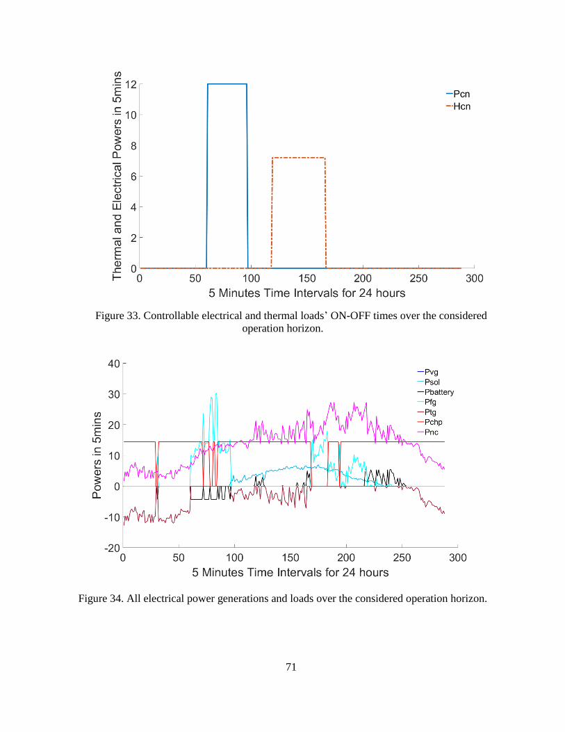
71
Figure 33. Controllable electrical and thermal loads’ ON-OFF times over the considered
operation horizon.
Figure 34. All electrical power generations and loads over the considered operation horizon.

72
Figure 35. All thermal power generations and loads over the considered operation horizon.
Case 3: Data-Driven Chance-Constrained Optimization with Flexibility Constraints
We apply the non-parametric chance-constrained method to manage the energy system taking
into account the flexibility constraints, i.e., ramping capabilities of energy storage for short-term
regulation purposes. By adding flexibility constraints, we can compare the results of the offered
algorithm with those obtained by the non-parametric chance-constrained optimization. That is,
constraints (9) – (16), (25), (26), (39) - (40), and (53) are considered in the energy management
optimization problem compared to the previous case. Thus, not only the storage participates in the
load following process, but also it provides adequate regulation reserve (i.e., fast-ramping reserve)
to ensure the system flexibility in response to the short-term solar power and load fluctuations.
Moreover, the battery follows the output power of PVs to make it smoother in answer to 5-mins

73
forecasting error of solar power. Similar to Case 2, we test three different scenarios (scenario1 =
50 samples, scenario2 = 100 samples, and scenario3 = 200 samples) at 95% confidence level.
Figure 36 and 37 illustrate the regulation reserve capacity (ramp up and down) over the
considered operation horizon. The required regulation reserve (MG’s requirements to ramp short-
term fluctuations) is also shown in these figures. Consider the results obtained by Case 2. In several
intervals (for instance, 210-240th intervals in Figure 36, and 60-100th intervals in Figure 37), the
available regulation reserve is less than the possible short-term fluctuations. Hence, in these
intervals, Case 2 has no adequate regulation reserve to respond to the short-term solar and load
fluctuations, and the system is at risk. In contrast to Case 2, in Case 3, we always have enough
regulation reserves to respond to possible short-term fluctuations and ensure the MG reliability
and security.
Figure 38 shows the battery charging/discharging pattern. This figure is for scenario 3 with
200 sample points when the confidence level is set to 95%. Since energy storage is deployed for
multiple purposes (i.e., energy arbitrage according to the price signal, load following in response
to solar generation and load forecasting errors, and regulation reserve to alleviate short-term solar
power and load fluctuations), charging and discharging patterns have several jumps to fulfill these
services. These patterns are different them in Case 2.
Figures 39-43 show battery energy status, power exchanged with the distribution feeder,
controllable loads, electricity generation and loads, and thermal power generations and load.
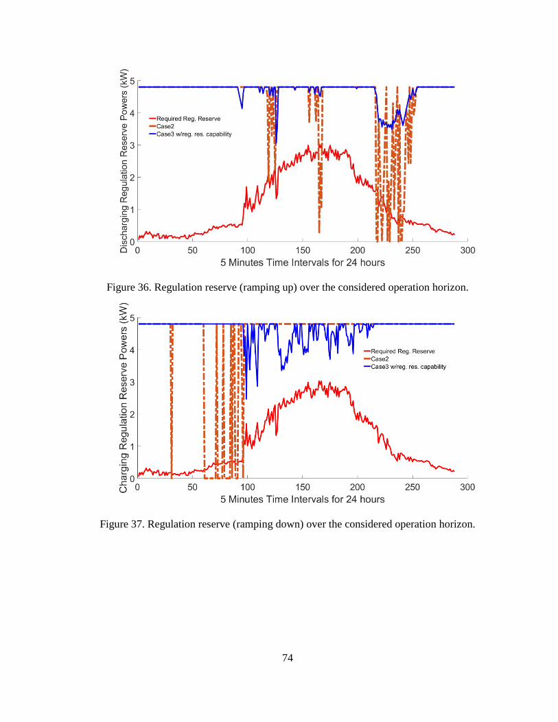
74
Figure 36. Regulation reserve (ramping up) over the considered operation horizon.
Figure 37. Regulation reserve (ramping down) over the considered operation horizon.

75
Figure 38. Non-parametric 200 samples battery charging and discharging powers with
ramping over the considered operation horizon.
Figure 39. State of charge of battery in percentage over the considered operation horizon.

76
Figure 40. The power buying from and selling to the distribution feeder over the considered
operation horizon.
Figure 41. Controllable electrical and thermal loads' ON-OFF times over the considered
operation horizon.

77
Figure 42. All electrical power generations and loads over the considered operation horizon.
Figure 43. All thermal power generations and loads over the considered operation horizon.
78
Moreover, the virtual power generation is included in Case 3 to smooth the solar power injected
to MG. Figure 44 demonstrates the solar power and the virtual generation output for scenario 3
(i.e., 200 samples) and 95% of confidence level. The solar power is represented by the dash-dot
brown line, and the continuous blue line is the output power of the virtual power generation. The
output of the virtual generation is smoother than the solar power.
Figure 44. Output of virtual power generation and solar power comparison with ramping over
the considered operation horizon.
Figure 45 and Table II show that the operation cost goes up by adding flexibility constraints.
Compared with Case 2, the operation cost of scenarios 1, 2, and 3 is increased from $26.66, $25.70,
and $24.08 to $27.05, $26.06, $24.39, respectively, at 90% confidence level. The operation cost
of scenario 1 is more than that obtained by the two other scenarios. Scenario 3 offers the least cost,
but not less than Case 2. The operation cost of DDCC is always larger than that for the parametric
model. Indeed, enlarging the sample size reduces the adjusted confidence level and makes it close

79
to the original confidence level. This consequently reduces the cost difference between obtained
by DDCC and the parametric model. This cost increment (Cost of DCCC – cost of the parametric
model) is interpreted as a cost that the MG operator pays to alleviate possible forecasting errors
and the short-term fluctuations and ensure the system security and reliability.
Figure 45. Total cost comparison of 50, 100, 200 samples with flexibility constraints, and
parametric.
Table II. Comparison between energy management costs obtained by parametric and non-
parametric methods with flexibility constraints.
Confidence
Level
Non-parametric Parametric
50 samples 100 samples 200 samples
90% 27.05 26.06 24.39 23.74
95% 28.96 27.61 26.85 24.70
99% 30.03 30.03 29.61 26.55
0
5
10
15
20
25
30
35
50 100 200 Param. 50 100 200 Param. 50 100 200 Param.
Co
st (
$)

80
CHAPTER 5. SUMMARY, CONCLUSION, AND FUTURE WORK
Summary
Increasing penetration level of distributed energy resources (DERs) in distribution systems has
brought the concept active distribution grids and microgrids into power systems operation. Solar
power is most popular DERs that have been widely used in microgrids. Although solar power is a
clean energy, microgrids face new challenges because of solar generation uncertainties. Energy
storage devices are key enablers for solar power integration to microgrids. However, storage is an
expensive device. One of the most important roles of battery storage devices is their capabilities
for providing multiple services to the grid. This can be leveraged to justify costs of energy storage.
This thesis proposes an energy management algorithm for community microgrids taking into
account solar generation uncertainties and the battery storage capabilities for proving multiple
services to the grid. Two type of energy, thermal and electrical, and various generation resources
and consumers are considered in the proposed model. The electricity generation sources consist of
the distribution feeder, photovoltaic (PV) cells, combined heat and power (CHP), battery storage;
and thermal power suppliers include CHP and boilers. The consumers are controllable/non-
controllable thermal and electrical loads. In Chapter 3, uncertainties of solar power and loads are
ignored, and a deterministic optimization is formulated for MG energy management. To ensure
the system security and reliability against short-term fluctuations, a set of flexibility constraints
are modeled. These flexibility constraints alleviate spreading short-term fluctuations of solar and
load to the distribution feeder. That is, the microgrid (smart building) is capable of capturing
fluctuations locally. In Chapter 4, solar generation and load forecast error and short-term
fluctuations are taken into consideration. A chance-constrained approach is presented to model
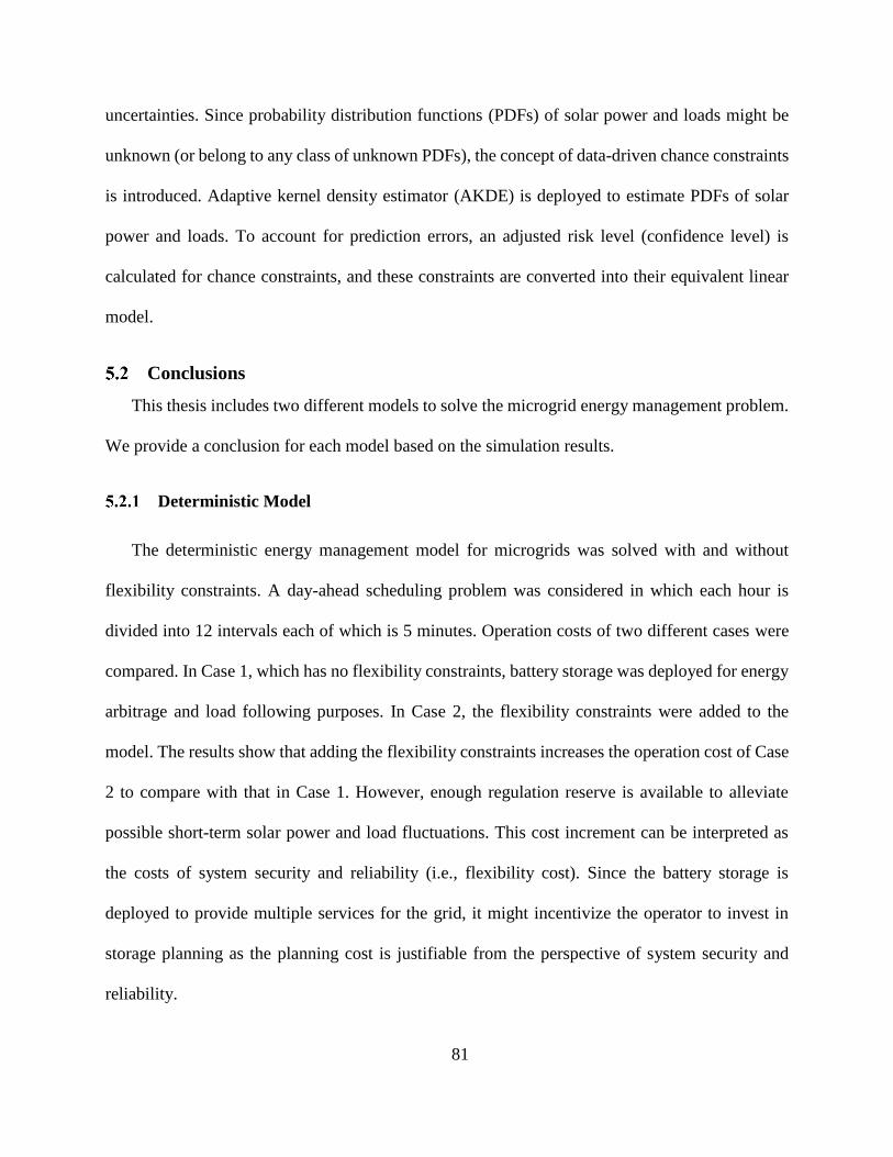
81
uncertainties. Since probability distribution functions (PDFs) of solar power and loads might be
unknown (or belong to any class of unknown PDFs), the concept of data-driven chance constraints
is introduced. Adaptive kernel density estimator (AKDE) is deployed to estimate PDFs of solar
power and loads. To account for prediction errors, an adjusted risk level (confidence level) is
calculated for chance constraints, and these constraints are converted into their equivalent linear
model.
Conclusions
This thesis includes two different models to solve the microgrid energy management problem.
We provide a conclusion for each model based on the simulation results.
Deterministic Model
The deterministic energy management model for microgrids was solved with and without
flexibility constraints. A day-ahead scheduling problem was considered in which each hour is
divided into 12 intervals each of which is 5 minutes. Operation costs of two different cases were
compared. In Case 1, which has no flexibility constraints, battery storage was deployed for energy
arbitrage and load following purposes. In Case 2, the flexibility constraints were added to the
model. The results show that adding the flexibility constraints increases the operation cost of Case
2 to compare with that in Case 1. However, enough regulation reserve is available to alleviate
possible short-term solar power and load fluctuations. This cost increment can be interpreted as
the costs of system security and reliability (i.e., flexibility cost). Since the battery storage is
deployed to provide multiple services for the grid, it might incentivize the operator to invest in
storage planning as the planning cost is justifiable from the perspective of system security and
reliability.

82
Probabilistic Model
We analyzed three cases to demonstrate the effectiveness of the proposed chance-constrained
model for microgrid energy management. Case 1 was aimed to solve the optimization problem
with the parametric chance-constrained method while flexibility constraints are not involved. Case
2 was solved with the non-parametric chance-constrained model without the flexibility constraints.
The results of Case 2 revealed that the cost was slightly boosted after changing method from the
parametric to the non-parametric (data-driven) chance-constrained since PDFs of random variables
were determined as known, whereas they have normal distribution in the parametric chance-
constrained model. The DDCC model’s accuracy enhances by increasing number of sample points
for the solar power and load (which are random variables). Although the cost goes up, the DDCC
provides realistic results that are closer to the optimal solution after the true realization of the
uncertainties. This reduces the system rescheduling costs, and consequently the total operation
costs compared with the parametric chance constraints in which an assumption is imposed on PDFs
(i.e., PDFs follow a normal distribution). In addition, imposing no assumption on PDFs enhances
the MG reliability during the real-time operation.
With adding flexibility constraints, Case 3 was solved with the DDCC method. Battery’s power
rating was used for load following and regulation purposes. The results show that the system has
adequate regulation reserves (provide by battery) to mitigate short-term solar power and load
fluctuations. Although the flexibility constraints increase the operation costs of Case 3 compared
to that for Case 2, this scheduling model ensures the system reliability in the real-time operation.
In a nutshell, the case studies in Chapter 4 demonstrate that the DDCC optimization makes the
energy management’s results more realistic and acceptable.

83
Table III summarizes the results of Chapter 3 and Chapter 4. The results can be interpreted in
two ways; namely, the impact of the flexibility constraints and utilizing the DDCC model. Both
implementations increase the day-ahead operation costs. The difference between the deterministic
and the chance-constrained models are considerable since the former method does not consider
uncertainties while the later method models uncertainties. The DDCC method with flexibility
constraints potentially enhances the system reliability and reduces the rescheduling cost, and this
consequently reduces the overall system day-ahead scheduling and real-time rescheduling costs.
Table III. Day-ahead scheduling costs (in $)
Confidence
Level
Non-parametric
Parametric Deterministic
50
samples
100
samples
200
samples
Without
Flexibility
Constraints
90% 26.66 25.7 24.08 23.74
18.76 95% 28.51 27.21 26.46 24.7
99% 29.54 29.54 29.14 26.55
With
Flexibility
Constraints
90% 27.05 26.06 24.39 23.74
19.25 95% 28.96 27.61 26.85 24.7
99% 30.03 30.03 29.61 26.55
Future Work
The following tasks are potential future research directions to enhance our proposed algorithm
and design a more efficient microgrid energy management algorithm:
1. Using different (and more advanced) techniques to reduce errors of the estimated PDFs of
solar generation and loads

84
2. Adding new generation units (e.g., diesel or gas engine generators) to alleviate the burden
of energy storage
3. Using historical real solar generation and load data to show efficiency of the data-driven
chance-constrained model
4. Expanding the proposed model for larger systems, such as power transmission and
distribution systems
5. Determining good confidence levels (risk levels) with respect to the MG’s characteristics
and requirements
6. Considering a smart building and allowing the building operator to determine and control
confidence levels
7. Applying a game-based energy trading approach between microgrids via energy hubs
85
REFERENCES
[1] E. I. Administration, Annual Energy Outlook 2012: With Projections to 2035. Government
Printing Office, 2012.
[2] A. Borghetti et al., "Short-term scheduling and control of active distribution systems with
high penetration of renewable resources," IEEE Systems Journal, vol. 4, no. 3, pp. 313-
322, 2010.
[3] S.-J. Ahn, S.-R. Nam, J.-H. Choi, and S.-I. Moon, "Power scheduling of distributed
generators for economic and stable operation of a microgrid," IEEE Transactions on Smart
Grid, vol. 4, no. 1, pp. 398-405, 2013.
[4] T. Logenthiran, D. Srinivasan, A. M. Khambadkone, and H. N. Aung, "Multiagent system
for real-time operation of a microgrid in real-time digital simulator," IEEE Transactions
on smart grid, vol. 3, no. 2, pp. 925-933, 2012.
[5] F. Safdarian, M. Ardehali, and G. Gharehpetian, "Ramp Rate Effect on Maximizing Profit
of a Microgrid Using Gravitational Search Algorithm," in Proceedings of The, 2014.
[6] M. Geidl, G. Koeppel, P. Favre-Perrod, B. Klockl, G. Andersson, and K. Frohlich, "Energy
hubs for the future," IEEE Power and Energy Magazine, vol. 5, no. 1, pp. 24-30, 2007.
[7] B. Sivaneasan, K. Nandha Kumar, K. T. Tan, and P. L. So, "Preemptive Demand Response
Management for Buildings," IEEE Transactions on Sustainable Energy, vol. 6, no. 2, pp.
346-356, 2015.
[8] A. Y. Saber and G. K. Venayagamoorthy, "Resource scheduling under uncertainty in a
smart grid with renewables and plug-in vehicles," IEEE systems journal, vol. 6, no. 1, pp.
103-109, 2012.
[9] R. A. Jabr, "Adjustable robust OPF with renewable energy sources," IEEE Transactions
on Power Systems, vol. 28, no. 4, pp. 4742-4751, 2013.
[10] A. Baziar and A. Kavousi-Fard, "Considering uncertainty in the optimal energy
management of renewable micro-grids including storage devices," Renewable Energy, vol.
59, no. Supplement C, pp. 158-166, 2013/11/01/ 2013.
[11] A. Kargarian, G. Hug, and J. Mohammadi, "A Multi-Time Scale Co-Optimization Method
for Sizing of Energy Storage and Fast-Ramping Generation," IEEE Transactions on
Sustainable Energy, vol. 7, no. 4, pp. 1351-1361, 2016.
[12] H. Kanchev, D. Lu, F. Colas, V. Lazarov, and B. Francois, "Energy Management and
Operational Planning of a Microgrid With a PV-Based Active Generator for Smart Grid
Applications," IEEE Transactions on Industrial Electronics, vol. 58, no. 10, pp. 4583-
4592, 2011.
86
[13] H. T. Nguyen, D. T. Nguyen, and L. B. Le, "Energy Management for Households With
Solar Assisted Thermal Load Considering Renewable Energy and Price Uncertainty,"
IEEE Transactions on Smart Grid, vol. 6, no. 1, pp. 301-314, 2015.
[14] P. Liu, Y. Fu, and A. Kargarian marvasti, "Multi-stage Stochastic Optimal Operation of
Energy-efficient Building with Combined Heat and Power System," Electric Power
Components and Systems, vol. 42, no. 3-4, pp. 327-338, 2014.
[15] Q. D. La, Y. W. E. Chan, and B.-H. Soong, "Power Management of Intelligent Buildings
Facilitated by Smart Grid: A Market Approach," IEEE Transactions on Smart Grid, vol.
7, no. 3, pp. 1389-1400, 2016.
[16] D. E. Olivares, J. D. Lara, C. A. Cañizares, and M. Kazerani, "Stochastic-Predictive Energy
Management System for Isolated Microgrids," IEEE Transactions on Smart Grid, vol. 6,
no. 6, pp. 2681-2693, 2015.
[17] Y. Zhang, N. Gatsis, and G. B. Giannakis, "Robust energy management for microgrids
with high-penetration renewables," IEEE Transactions on Sustainable Energy, vol. 4, no.
4, pp. 944-953, 2013.
[18] W. Wei, F. Liu, and S. Mei, "Energy pricing and dispatch for smart grid retailers under
demand response and market price uncertainty," IEEE transactions on smart grid, vol. 6,
no. 3, pp. 1364-1374, 2015.
[19] A. Charnes and W. W. Cooper, "Chance-constrained programming," Management science,
vol. 6, no. 1, pp. 73-79, 1959.
[20] A. Shapiro and A. Philpott, "A tutorial on stochastic programming," Manuscript. Available
at www2. isye. gatech. edu/ashapiro/publications. html, vol. 17, 2007.
[21] M. Parvania and M. Fotuhi-Firuzabad, "Demand response scheduling by stochastic
SCUC," IEEE Transactions on smart grid, vol. 1, no. 1, pp. 89-98, 2010.
[22] N. Growe-Kuska, H. Heitsch, and W. Romisch, "Scenario reduction and scenario tree
construction for power management problems," in Power tech conference proceedings,
2003 IEEE Bologna, 2003, vol. 3, p. 7 pp. Vol. 3: IEEE.
[23] M. H. Moradi, M. Eskandari, and S. Mahdi Hosseinian, "Operational Strategy
Optimization in an Optimal Sized Smart Microgrid," IEEE Transactions on Smart Grid,
vol. 6, no. 3, pp. 1087-1095, 2015.
[24] Y. Zhang, N. Gatsis, and G. B. Giannakis, "Risk-constrained energy management with
multiple wind farms," in Innovative Smart Grid Technologies (ISGT), 2013 IEEE PES,
2013, pp. 1-6: IEEE.

87
[25] J. Liu, M. G. Martinez, B. Li, J. Mathieu, and C. L. Anderson, "A comparison of robust
and probabilistic reliability for systems with renewables and responsive demand," in
System Sciences (HICSS), 2016 49th Hawaii International Conference on, 2016, pp. 2373-
2380: IEEE.
[26] A. Abdulkarim, S. M. Abdelkader, and D. John Morrow, "Statistical Analyses of Wind and
Solar Energy Resources for the Development of Hybrid Microgrid," pp. 9-14, 2015.
[27] M. Kazemi, H. Zareipour, N. Amjady, W. D. Rosehart, and M. Ehsan, "Operation
Scheduling of Battery Storage Systems in Joint Energy and Ancillary Services Markets,"
IEEE Transactions on Sustainable Energy, 2017.
[28] Y. Huang, L. Wang, W. Guo, Q. Kang, and Q. Wu, "Chance Constrained Optimization in
a Home Energy Management System," IEEE Transactions on Smart Grid, vol. PP, no. 99,
pp. 1-1, 2017.
[29] M. Josephson, "Edison: A Biography (New York, 1959)," The Robber Barons: The Great
American Capitalists, vol. 1901, 1861.
[30] (2011). U.S. Dept. of Energy, DOE Microgrid Workshop Report. Available:
http://energy.gov/sites/prod/files/Microgrid%20Workshop%20Report%20August%20201
1.pdf
[31] Q. Li, Z. Xu, and L. Yang, "Recent advancements on the development of microgrids,"
Journal of Modern Power Systems and Clean Energy, vol. 2, no. 3, pp. 206-211, 2014.
[32] E. Hayden, "Introduction to microgrids," Securicon Report, pp. 1-13, 2013.
[33] M. M. Hand, Renewable electricity futures study. National Renewable Energy Laboratory,
2012.
[34] A. Khodaei, S. Bahramirad, and M. Shahidehpour, "Microgrid Planning Under
Uncertainty," IEEE Transactions on Power Systems, vol. 30, no. 5, pp. 2417-2425, 2015.
[35] A. Khodaei, "Provisional Microgrid Planning," IEEE Transactions on Smart Grid, vol. 8,
no. 3, pp. 1096-1104, 2017.
[36] L. Che, X. Zhang, M. Shahidehpour, A. Alabdulwahab, and A. Abusorrah, "Optimal
Interconnection Planning of Community Microgrids With Renewable Energy Sources,"
IEEE Transactions on Smart Grid, vol. 8, no. 3, pp. 1054-1063, 2017.
[37] H. Wang and J. Huang, "Cooperative Planning of Renewable Generations for
Interconnected Microgrids," IEEE Transactions on Smart Grid, vol. 7, no. 5, pp. 2486-
2496, 2016.

88
[38] M. M. A. Abdelaziz, H. E. Farag, and E. F. El-Saadany, "Optimum Reconfiguration of
Droop-Controlled Islanded Microgrids," IEEE Transactions on Power Systems, vol. 31,
no. 3, pp. 2144-2153, 2016.
[39] B. Davito, H. Tai, and R. Uhlaner, "The smart grid and the promise of demand-side
management," McKinsey on Smart Grid, vol. 3, pp. 8-44, 2010.
[40] I. K. Maharjan, Demand side management: Load management, load profiling, load
shifting, residential and industrial consumer, energy audit, reliability, urban, semi-urban
and rural setting. LAP Lambert Academic Publ, 2010.
[41] C. W. Gellings and J. Chamberlin, "Demand-side management," ed: Boca Raton, FL, USA:
CRC Press, 1988.
[42] T. Logenthiran, D. Srinivasan, and T. Z. Shun, "Demand side management in smart grid
using heuristic optimization," IEEE transactions on smart grid, vol. 3, no. 3, pp. 1244-
1252, 2012.
[43] J. Shen, C. Jiang, and B. Li, "Controllable Load Management Approaches in Smart Grids,"
Energies, vol. 8, no. 10, pp. 11187-11202, 2015.
[44] C. W. Gellings, "The concept of demand-side management for electric utilities,"
Proceedings of the IEEE, vol. 73, no. 10, pp. 1468-1470, 1985.
[45] P. Palensky and D. Dietrich, "Demand Side Management: Demand Response, Intelligent
Energy Systems, and Smart Loads," IEEE Transactions on Industrial Informatics, vol. 7,
no. 3, pp. 381-388, 2011.
[46] M. H. Albadi and E. F. El-Saadany, "A summary of demand response in electricity
markets," Electric Power Systems Research, vol. 78, no. 11, pp. 1989-1996, 2008.
[47] N. Li, L. Chen, and S. H. Low, "Optimal demand response based on utility maximization
in power networks," in 2011 IEEE Power and Energy Society General Meeting, 2011, pp.
1-8.
[48] V. VDI-Guideline, "4602," ed: Beuth Verlag, Berlin, 2007, p. 3.
[49] M. Pipattanasomporn, M. Kuzlu, and S. Rahman, "An Algorithm for Intelligent Home
Energy Management and Demand Response Analysis," IEEE Transactions on Smart Grid,
vol. 3, no. 4, pp. 2166-2173, 2012.
[50] T. Wang, Y. Xu, C. Withanage, L. Lan, S. Ahipasaoglu, and C. Courcoubetis, "A Fair and
Budget-Balanced Incentive Mechanism for Energy Management in Buildings," IEEE
Transactions on Smart Grid, pp. 1-1, 2016.
89
[51] C. Keerthisinghe, G. Verbic, and A. C. Chapman, "A Fast Technique for Smart Home
Management: ADP with Temporal Difference Learning," IEEE Transactions on Smart
Grid, pp. 1-1, 2016.
[52] M. Rastegar, M. Fotuhi-Firuzabad, and M. Moeini- Aghtaie, "Developing a Two-Level
Framework for Residential Energy Management," IEEE Transactions on Smart Grid, pp.
1-1, 2016.
[53] B. Chai, A. Costa, S. D. Ahipasaoglu, C. Yuen, and Z. Yang, "Optimal Meeting Scheduling
in Smart Commercial Building for Energy Cost Reduction," IEEE Transactions on Smart
Grid, pp. 1-1, 2016.
[54] D. Zhang, S. Li, M. Sun, and Z. O'Neill, "An Optimal and Learning-Based Demand
Response and Home Energy Management System," IEEE Transactions on Smart Grid, vol.
7, no. 4, pp. 1790-1801, 2016.
[55] P. Arboleya et al., "Efficient Energy Management in Smart Micro-Grids: ZERO Grid
Impact Buildings," IEEE Transactions on Smart Grid, vol. 6, no. 2, pp. 1055-1063, 2015.
[56] K. Kampouropoulos, F. Andrade, E. Sala, A. Garcia Espinosa, and J. L. Romeral,
"Multiobjective Optimization of Multi-Carrier Energy System using a Combination of
ANFIS and Genetic Algorithms," IEEE Transactions on Smart Grid, pp. 1-1, 2016.
[57] A. Najafi, H. Falaghi, J. Contreras, and M. Ramezani, "A Stochastic Bilevel Model for the
Energy Hub Manager Problem," IEEE Transactions on Smart Grid, vol. 8, no. 5, pp. 2394-
2404, 2017.
[58] M. Moeini-Aghtaie, H. Farzin, M. Fotuhi-Firuzabad, and R. Amrollahi, "Generalized
Analytical Approach to Assess Reliability of Renewable-Based Energy Hubs," IEEE
Transactions on Power Systems, vol. 32, no. 1, pp. 368-377, 2017.
[59] M. Batić, N. Tomašević, G. Beccuti, T. Demiray, and S. Vraneš, "Combined energy hub
optimisation and demand side management for buildings," Energy and Buildings, vol. 127,
pp. 229-241, 2016.
[60] J. Wang, X. Wang, and Y. Wu, "Operating Reserve Model in the Power Market," IEEE
Transactions on Power Systems, vol. 20, no. 1, pp. 223-229, 2005.
[61] X. Yan, B. Francois, and D. Abbes, "Operating power reserve quantification through PV
generation uncertainty analysis of a microgrid," in 2015 IEEE Eindhoven PowerTech,
2015, pp. 1-6.
[62] B. D. H. Kiran and M. S. Kumari, "Optimal generation scheduling with operating reserves
including wind uncertainties," in 2014 International Conference on Smart Electric Grid
(ISEG), 2014, pp. 1-6.
90
[63] H. Holttinen et al., "Methodologies to determine operating reserves due to increased wind
power," in 2013 IEEE Power & Energy Society General Meeting, 2013, pp. 1-10.
[64] "NERC Distributed Energy Resources Report," 2017, Available:
http://www.nerc.com/comm/Other/essntlrlbltysrvcstskfrcDL/Distributed_Energy_Resour
ces_Report.pdf.
[65] "Andersen, Reprinted from Public Utility Reports, Inc., from the Summer 2001; issue of
Fortnightly‘s Energy Customer Management.."
[66] F. Golestaneh, P. Pinson, and H. B. Gooi, "Very Short-Term Nonparametric Probabilistic
Forecasting of Renewable Energy Generation— With Application to Solar Energy," IEEE
Transactions on Power Systems, vol. 31, no. 5, pp. 3850-3863, 2016.
[67] Z. Xiangqi, Y. Jiahong, and L. Ning, "A probabilistic-based PV and energy storage sizing
tool for residential loads," in 2016 IEEE/PES Transmission and Distribution Conference
and Exposition (T&D), 2016, pp. 1-5.
[68] T. Schittekatte, M. Stadler, G. Cardoso, S. Mashayekh, and N. Sankar, "The impact of
short-term stochastic variability in solar irradiance on optimal microgrid design," IEEE
Transactions on Smart Grid, vol. PP, no. 99, pp. 1-1, 2017.
[69] T. A. Nguyen and M. L. Crow, "Stochastic Optimization of Renewable-Based Microgrid
Operation Incorporating Battery Operating Cost," IEEE Transactions on Power Systems,
vol. 31, no. 3, pp. 2289-2296, 2016.
[70] E. Yao, P. Samadi, V. W. S. Wong, and R. Schober, "Residential Demand Side
Management Under High Penetration of Rooftop Photovoltaic Units," IEEE Transactions
on Smart Grid, vol. 7, no. 3, pp. 1597-1608, 2016.
[71] A. Kargarian and G. Hug, "Optimal sizing of energy storage systems: a combination of
hourly and intra-hour time perspectives," IET Generation, Transmission & Distribution,
vol. 10, no. 3, pp. 594-600, 2016.
[72] J. Zhuang, G. Shen, J. Yu, T. Xiang, and X. Wang, "Micro-Grid Energy Storage Location
and Sizing Optimization Method Based on Demand Response," in 2016 International
Conference on Intelligent Transportation, Big Data & Smart City (ICITBS), 2016, pp. 517-
520.
[73] Y. V. Makarov, C. Loutan, M. Jian, and P. de Mello, "Operational Impacts of Wind
Generation on California Power Systems," IEEE Transactions on Power Systems, vol. 24,
no. 2, pp. 1039-1050, 2009.
[74] B. Jintanasombat and S. Premrudeepreechacharn, "Optimal analysis of battery energy
storage for reduction of power fluctuation from PV system in Mae Hong Son province," in
2015 5th International Youth Conference on Energy (IYCE), 2015, pp. 1-6.

91
[75] C. E. "Cogeneration | Combined heat and power | CHP | Cogen", 2017. [Online]. Available:
https://www.clarke-energy.com/chp-cogeneration/.
[76] Z. Li, W. Wu, M. Shahidehpour, J. Wang, and B. Zhang, "Combined Heat and Power
Dispatch Considering Pipeline Energy Storage of District Heating Network," IEEE
Transactions on Sustainable Energy, vol. 7, no. 1, pp. 12-22, 2016.
[77] E. A. Duki, "Optimal sizing of CHP for residential complexes by two-stage stochastic
programming," in 2012 Proceedings of 17th Conference on Electrical Power Distribution,
2012, pp. 1-5.
[78] D. Xie, Y. Lu, J. Sun, C. Gu, and G. Li, "Optimal Operation of a Combined Heat and Power
System Considering Real-time Energy Prices," IEEE Access, vol. 4, pp. 3005-3015, 2016.
[79] A. Ben-Tal, L. El Ghaoui, and A. Nemirovski, Robust optimization. Princeton University
Press, 2009.
[80] J. R. Birge and F. Louveaux, Introduction to stochastic programming. Springer Science &
Business Media, 2011.
[81] W. B. Powell, Approximate Dynamic Programming: Solving the curses of dimensionality.
John Wiley & Sons, 2007.
[82] B. A. Calfa, I. E. Grossmann, A. Agarwal, S. J. Bury, and J. M. Wassick, "Data-driven
individual and joint chance-constrained optimization via kernel smoothing," Computers &
Chemical Engineering, vol. 78, pp. 51-69, 2015.
[83] R. Henrion, "Introduction to chance-constrained programming," Tutorial paper for the
Stochastic Programming Community home page, 2004.
[84] W. J. Dixon and J. Massey Frank, Introduction To Statistical Analsis. McGraw-Hill Book
Company, Inc; New York, 1950.
[85] H. Wu, M. Shahidehpour, Z. Li, and W. Tian, "Chance-Constrained Day-Ahead
Scheduling in Stochastic Power System Operation," IEEE Transactions on Power Systems,
vol. 29, no. 4, pp. 1583-1591, 2014.
[86] J. Liu, H. Chen, W. Zhang, B. Yurkovich, and G. Rizzoni, "Energy Management Problems
Under Uncertainties for Grid-Connected Microgrids: a Chance Constrained Programming
Approach," IEEE Transactions on Smart Grid, vol. PP, no. 99, pp. 1-1, 2017.
[87] R. Jiang and Y. Guan, "Data-driven chance constrained stochastic program," Mathematical
Programming, vol. 158, no. 1-2, pp. 291-327, 2016.
92
[88] A. Ben-Tal, D. Den Hertog, A. De Waegenaere, B. Melenberg, and G. Rennen, "Robust
solutions of optimization problems affected by uncertain probabilities," Management
Science, vol. 59, no. 2, pp. 341-357, 2013.
[89] H. Hejazi and H. Mohsenian-Rad, "Energy Storage Planning in Active Distribution Grids:
A Chance-Constrained Optimization with Non-Parametric Probability Functions," IEEE
Transactions on Smart Grid, pp. 1-1, 2016.
[90] L. Oneto, F. Laureri, M. Robba, F. Delfino, and D. Anguita, "Data-Driven Photovoltaic
Power Production Nowcasting and Forecasting for Polygeneration Microgrids," IEEE
Systems Journal, pp. 1-12, 2017.
[91] C. Zhao and Y. Guan, "Data-Driven Stochastic Unit Commitment for Integrating Wind
Generation," IEEE Transactions on Power Systems, vol. 31, no. 4, pp. 2587-2596, 2016.
[92] K. X. Perez et al., "Soft-islanding a group of houses through scheduling of CHP, PV and
storage," in 2016 IEEE International Energy Conference (ENERGYCON), 2016, pp. 1-6.
[93] J. Lofberg, "YALMIP: A toolbox for modeling and optimization in MATLAB," in
Computer Aided Control Systems Design, 2004 IEEE International Symposium on, 2004,
pp. 284-289: IEEE.
[94] Z. I. Botev, J. F. Grotowski, and D. P. Kroese, "Kernel density estimation via diffusion,"
The Annals of Statistics, vol. 38, no. 5, pp. 2916-2957, 2010.

93
VITA
Okan Ciftci was born in Konya, Turkey. He received the Bachelor Degree in Electrical and
Electronics Engineering from KTO Karatay University, Konya, Turkey, in 2014. After receiving
B.S. degree, he was awarded a full scholarship from the Turkish Ministry of Education for his
Master’s and Ph.D. studies in the US. He has been working towards his MSc degree in the
department of Electrical Engineering at Louisiana State University, Baton Rouge, Louisiana since
2016. His research interests are optimization of power systems operation, generation, and
scheduling.


![Joint Investment and Operation of Microgrid · 2015-11-09 · and microgrid operation. While in [9]–[12], only microgrid operation is studied under given microgrid facilities. However,](https://static.documents.pub/doc/80x56/5f055ca67e708231d412960b/joint-investment-and-operation-of-microgrid-2015-11-09-and-microgrid-operation.jpg)


