
1
MODEL VALIDATION VIA UNCERTAINTY PROPAGATION AND DATA
TRANSFORMATIONS
Wei Chen*
Integrated Design Automation Laboratory (IDEAL)
Department of Mechanical Engineering
Northwestern University
Lusine Baghdasaryan
Department of Mechanical & Industrial Engineering
University of Illinois at Chicago
Thaweepat Buranathiti and Jian Cao
Advanced Materials Processing Laboratory
Department of Mechanical Engineering
Northwestern University
Evanston, Illinois
* Corresponding Author, Mechanical Engineering, Northwestern University 2145 Sheridan Road, Tech B224, Evanston, IL 60208-3111; Phone: (847) 491-7019, Fax: (847) 491-3915; email: [email protected].
Revision 2
Submitted to the AIAA Journal
December 2003
2
Abstract
Model validation has become a primary means to evaluate accuracy and reliability of
computational simulations in engineering design. Due to uncertainties involved in modeling,
manufacturing processes, and measurement systems, the assessment of the validity of a modeling
approach must be conducted based on stochastic measurements to provide designers with the
confidence of using a model. In this paper, a generic model validation methodology via
uncertainty propagation and data transformations is presented. The approach reduces the number
of physical tests at each design setting to one by shifting the evaluation effort to uncertainty
propagation of the computational model. Response surface methodology is used to create
metamodels as less costly approximations of simulation models for the uncertainty propagation.
Methods for validating models with both normal and nonnormal response distributions are
proposed. The methodology is illustrated with the examination of the validity of two finite
element analysis models for predicting springback angles in a sample flanging process.
Key words: Model validation, Uncertainty propagation, Response surface models, Sheet metal
forming, Data transformations.
1. INTRODUCTION
The increased dependence on using computer simulation models in engineering design arises a
critical issue of confidence in modeling and simulation accuracy. Model verification and
validation are the primary methods for building and quantifying confidence, as well as for the
demonstration of correctness of a model [1], [2]. Briefly, model verification is the assessment of
the solution accuracy of a mathematical model. Model validation, on the other hand, is the

3
assessment of how accurately the mathematical model represents the real world application [3].
Thus, in verification, the relationship of the simulation to the real world is not an issue, while in
validation, the relationship between the virtual (computation) and the real world, i.e.,
experimental data, is the issue.
One limitation of the existing model validation approaches is that they are restricted to the
validation at a particular design setting. There is no guarantee that the conclusion can be
extended over the entire design space. In addition, model validations are frequently based on
comparisons between the output from deterministic simulations and that from single or repeated
experiments. The existing statistical approaches, for which the physical experiment has to be
repeated a sufficient number of independent times, is not practical for many applications, simply
due to the cost and time commitment associated with experiments. Furthermore, deterministic
simulations for model validation do not consider uncertainty at all. Although recent model
validation approaches propose to shift the effort to propagating the uncertainty in model
predictions, which implies that a model validation should include all relevant sources of
uncertainties, little work has been accomplished in this area [1], [2], [4]. Since realistic
mathematical models should contemplate uncertainties, the assessment of the validity of a
modeling approach must be conducted based on stochastic measurements to provide designers
with the confidence of using a model.
Traditionally, a model has been considered valid if it reproduces the results with adequate
accuracy. The two traditional model validation approaches are: 1) subjective and 2) quantitative
comparisons of model predictions and experimental observations. Subjective comparisons are

4
through visual inspection of x-y plots, scatter plots and contour plots. Though they show the
trend in data over time and space, subjective comparisons depend on graphical details.
Quantitative comparisons, including the measures of correlation coefficient and other weighted
and non-weighted norms, quantify the “distance” but become very subjective when defining
what magnitudes of the measures are acceptable. To quantify model validity from a stochastic
perspective, researchers have proposed various statistical inference techniques, such as χ2 test on
residuals between model and experimental results [5]. These statistical inferences require
multiple evaluations of the model and experiments, and many assumptions that are difficult to
satisfy. Therefore, there is a need for a model validation approach that takes the least amount of
statistical assumptions and requires the minimum number of physical experiments.
In this paper, we present a rigorous and practical approach for model validation (Model
Validation via Uncertainty Propagation) that utilizes the knowledge of system variations along
with computationally efficient uncertainty propagation techniques to provide a stochastic
assessment of the validity of a modeling approach for a specified design space. Various sources
of uncertainties in modeling and in physical tests are evaluated and the number of physical
testing at each design setting is reduced to ONE. Response surface methodology is used to create
a metamodel of an original simulation model, and therefore, the computational effort for
uncertainty propagation is reduced. By employing data transformations, the approach can also be
applied to the response distributions that are non-normal. This helps us represent the data in a
form that satisfies the assumptions underlying the r2 method, an approach used in this work to
determine whether the results from physical experiments fall inside or outside of the prespecified
confidence region. Even though the proposed methodology is demonstrated for validating two
5
finite-element models for simulating sheet metal forming, namely a flanging process, it can be
generalized to other engineering problems.
This paper is organized as follows. In Section 2, the technical background of this research is
provided. The major types of uncertainties in modeling are first introduced and classified into
three categories. Existing techniques on uncertainty propagation are then reviewed, the
background of the response surface methodology and statistical data transformations are
provided. Our proposed model validation approach is described in Section 3. In Section 4, our
proposed approach is demonstrated using a case study in sheet metal forming by examining two
finite element based models. Finally, conclusions are provided in Section 5.
2. TECHNICAL BACKGROUND
2.1 CLASSIFICATION OF UNCERTAINTIES
Various types of uncertainties exist in any physical system and in its modeling process and can
affect the final experimental or predicted system response. Different ways of classifying
uncertainties have been seen in the literature [6]-[9]. In this work, we classify uncertainties into
three major categories:
• Type I: Uncertainty associated with the inherent variation in the physical system or
environment that is under consideration. For example, uncertainty associated with incoming
material, initial part geometry, tooling setup, process setup, and operating environment.
• Type II: Uncertainty associated with deficiency in any phase or activity of the simulation
process that originates in lack of system knowledge. For example, uncertainty associated

6
with the lack of knowledge in the laws describing the behavior of the system under various
conditions, etc.
• Type III: Uncertainty associated with error that belongs to recognizable deficiency but is not
due to lack of knowledge. For example, uncertainty associated with the limitations of
numerical methods used to construct simulation models.
When providing the stochastic assessment of model validity, all these three types of uncertainties
should be taken into account.
2.2 TECHNIQUES FOR UNCERTAINTY PROPAGATION
The use of an analysis approach to estimate the effect of uncertainties on model prediction is
referred to as uncertainty propagation. Several categories of methods exist in the literature. The
first category is the conventional sample-based approach such as Monte Carlo Simulations
(MCS). Although alternative sampling techniques such as Quasi Monte Carlo Simulations
including Halton sequence [10], Hammersley sequence [11], and Latin Supercube Sampling [12]
have been proposed, none of these techniques are computationally feasible for problems that
require complex computer simulations, each taking at least a few minutes or even hours or days.
Validating a modeling approach at multiple design settings becomes computationally infeasible.
The second category of uncertainty propagation approach is based on sensitivity analysis. Most
of these methods only provide the information of mean and variance based on approximations.
The level of accuracy is not sufficient for applications in model validation. Here, we propose to
use a response surface model (or metamodel) to replace the numerical model for uncertainty
propagation. The response surface model is generated as a function of design variables and

7
parameters. Monte Carlo Simulations are later performed using the response surface model as a
surrogate of the original numerical program. Details of response surface methodologies are
provided in the next section.
2.3 RESPONSE SURFACE METHODOLOGIES
Response surface methodologies are well known approaches for constructing approximation
models based on either physical experiments or computer experiments (simulations) [13]. Our
interest in this work is the latter where computer experiments are conducted by simulating the to-
be-validated model to build response surface models. They are often referred to as metamodels
as they provide a “model of the model” [14], replacing the expensive simulation models during
the design and optimization process. In this paper, response surface models based on simulation
results from finite element models are constructed and tested for model validation by using two
response surface modeling methods: Polynomial Regression (PR) and Kriging Methods (KG).
Polynomial regression models have been applied by a number of researchers [15], [16], in
designing complex engineering systems. In spite of the advantage obtained from the smoothing
capability of polynomial regression for noisy functions, there is always a drawback when
applying PR to model highly nonlinear behaviors. Higher-order polynomials can be used;
however, instabilities may arise [17], or it may be too difficult to take sufficient sample data to
estimate all coefficients in the polynomial equation, particularly in large dimensions.
A Kriging model [18] postulates a combination of a polynomial model and departures from it,
where the latter is assumed to be a realization of a stochastic process with a zero mean and a
8
spatial correlation function. A variety of correlation functions can be chosen [19], the Gaussian
correlation function proposed in is the most frequently used. The Kriging method is extremely
flexible to capture any type of nonlinear behaviors due to the wide range of the correlation
functions. The major disadvantages of the Kriging process are that model construction can be
very time-consuming and could be ill-conditioned [20].
In our earlier works, the advantages and limitations of various metamodeling techniques have
been examined using multiple modeling criteria and multiple test problems [21], [22]. Our
strategy in this work is to first fit a second-order polynomial model. If the accuracy is not
satisfactory, the Kriging method will be employed; otherwise the low-cost polynomial model
will be used for uncertainty propagation and model validation.
2.4. DATA TRANSFORMATIONS
Many statistical tests are based on the assumption of normality. When data deviate from
normality, an appropriate transformation can often yield a data set that does follow
approximately a normal distribution [23]. Generally, response distributions obtained from
uncertainty propagation at multiple design points may not be normal. Data transformations are
therefore employed in order to use the proposed validation approach that is based on the
normality assumption.
One of the most common and simplistic parametric transformation families studied by Tukey
[24] and later modified by Box and Cox [25] is:

9
0,log
;0,1)(
==
≠−
=
λ
λλ
λλ
Z
ZZ (1)
where λ is the transformation parameter. For different values of λ different transformations are
obtained. When λ = 1, no transformation occurs. When λ <1, the transformation makes the
variance of residuals smaller at large Z’s, and makes it larger at small Z’s. When λ>1, it has the
opposite effects of λ <1. When λ = 0, natural logarithm is used (see equation 1).
The Box-Cox transformation in equation (1), called the power transformation, is only
appropriate for positive data. Hinkley [26], Manly [27], John and Draper [28], and Yeo and
Johnson [29] proposed alternative families of transformations that can be used to compensate the
restrictions on Z, to obtain an approximate symmetry or to make the distribution closer to
normal.
The parameters of a transformation, e.g. λ, can be selected through a trial and error approach
until good normal probability plots are obtained, through optimization based on Maximum
Likelihood estimation or Bayesian estimation [25], likelihood ratio test [30] , or the use of M-
estimators [31], etc. Atkinson and Riani [32] and Krzanowski [33] discussed some aspects of
multivariate data transformations in more detail.
It is often more useful to apply transformations of predictor (model input) variables, along with
the transformations of the dependent (model output) variables. Box and Tidwell [35] provided an
iterative procedure to estimate appropriate transformations of the original model inputs.

10
Atkinson and Riani [32] discussed different models and reasons for what transformations of
predictor variables can be applied. It should also be noted that applying the existing
transformation techniques may have little effect if the values of the response are far from zero
and the scatter in the observations is relatively small (in other words, the ratio of the largest to
smallest observation should not be too close to one) [30].
3. OUR PROPOSED MODEL VALIDATION APPROACH
3.1 General Description of the Approach
Our proposed model validation approach is illustrated in Figure 1. The whole process includes
four major phases, in which Phase II and Phase III can be implemented in parallel. Phase I is the
Problem Setup stage. Here, uncertainties of all types described in Section 2.1 are investigated;
probabilistic descriptions of model inputs are established. With the aim of model validation over
a design space rather than at a single design point, sample design settings, represented by xi, i =
1…n, are formed using different combinations of values of design variables. The sampling can be
based on the knowledge of critical combinations of design variables at different levels, the
standard statistical techniques such as Design of Experiments (DOE) [13], or other methods for
efficient data sampling (e.g., optimal Latin Hyper Cube [37]). These techniques will be useful in
reducing the size of samples when the number of design variables considered is large.
Phase II is the (Physical) Experimental stage. One of the cornerstones of this proposed approach
is the minimum number of physical tests required. Physical experiments will be performed only
once at each design setting identified in Phase I. Measurements are taken for the model
11
responses that are of interest. The results of experiments are denoted as Yi, i = 1,…, n. Errors of
measurements are predicted.
Phase III (Model Uncertainty Propagation) is the stage for uncertainty propagation based on the
to-be-tested (computational) model. For computationally expensive models, we propose to first
construct a response surface model based on samples of numerical simulation results. Techniques
introduced in Section 2.3 can be applied here. Next, the total uncertainty of the response
prediction is analyzed using the response surface model through Monte Carlo Simulations
(MCS) introduced as following. It should be noted that for model validation at multiple design
points, uncertainty of the response prediction needs to be evaluated for each of the design points
as identified in Phase I.
The uncertainty of the (computational) model prediction can be evaluated by uncertainty
propagation using MCS applied to the metamodel (in this case, response surface model),
following the uncertainty descriptions identified in Phase I. When a sufficient number of
simulations are performed, the MCS is robust in a sense that it provides good estimates of
uncertainty in the predicted parameters, no matter whether the model is highly nonlinear or not.
The MCS also provides estimates of the shape of the probability density functions (pdf), which
are used further in Phase IV for model validation. If the normality checks for the pdf’s from
MCS are rejected, we propose to apply data transformations to data from the simulation models
before constructing response surface models so that the transformed distributions become
normal.
Insert Figure 1. Procedure for Model Validation
12
Phase IV is the Model Validation phase, when the stochastic assessment of model validity is
drawn based on the comparisons of the physical experimental results from Phase II and the
computational results from Phase III. The strategies introduced by Hills et al. [1] are followed
here. As Hills’ validation criterion for multiple design settings is applicable only for normal
response distributions, data transformation is proposed in this work to extend the applicability of
the proposed approach to non-normal response distributions. Details of model validation
strategies for single and multiple design points, procedures for data transformation, and
accounting various sources of errors are discussed next.
3.2 Model validation at a single design point
Hills’ method states that for a given confidence bound (say 100*(1-α%)), if the physical
experiment falls within the performance range obtained from the computer model (here, the
probability density function (pdf) obtained from the MCS in Phase III), it indicates that the
model is consistent with the experimental result (however, we can not say the model is valid for
the confidence bound). On the other hand, if one physical experiment is outside of the
performance range, then we would reject the model for that specified confidence bound (100*(1-
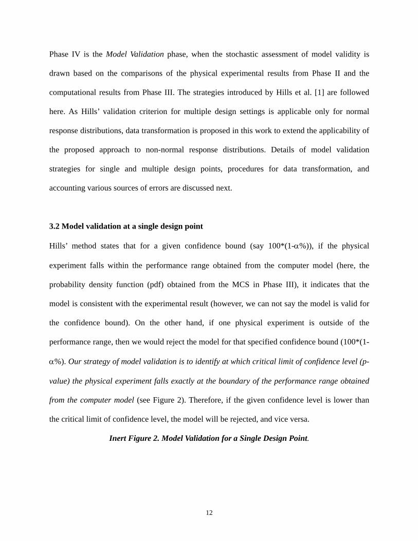
α%). Our strategy of model validation is to identify at which critical limit of confidence level (p-
value) the physical experiment falls exactly at the boundary of the performance range obtained
from the computer model (see Figure 2). Therefore, if the given confidence level is lower than
the critical limit of confidence level, the model will be rejected, and vice versa.
Inert Figure 2. Model Validation for a Single Design Point.
13
As shown illustratively in Figure 2, the probability density function describes the distribution of
a response based on the (computational) model for the given uncertainty description at a single
design point. The confidence limit with which one cannot reject the simulation model is the area
under the pdf curve that bounds exactly on the physical experiment, includes the mean of the
pdf, and excludes the two equally sized tails that depend on the location of the physical
experiment. If the confidence limit is identified as γ% which is smaller than the given confidence
bound (e.g., 100*(1-α)% in Figure 2), we cannot reject the model for an experiment that falls on
the boundary of γ%; otherwise we can reject the model since the physical experiment falls
outside the distribution range. When a model is rejected, it indicates that a new model needs to
be constructed and the whole procedure of model validation should be carried out again. It
should be noted that since stochastic assessments are provided for model validity, there are
certain risks associated with the error of hypothesis testing [38]. In our case, the false positive
error (commonly referred to as a Type I error) is the error of rejecting a model while the true
state is that the model is indeed valid. The probability of leading to this outcome is α%. We note
that providing a higher confidence bound (lower α%) would widen our acceptance region, while
it will reduce our chances of rejecting a valid model, it would also increase our chance of
accepting an invalid model, i.e., increasing the probability of making the false negative error
(referred to as a Type II error). Indications of Type I and Type II errors in model validation were
discussed by Oberkampf and Trucano [2], where they related the Type I error to a model
builder’s risk and Type II error to model users’ risk.
14
3.3 Model validation at multiple design settings
When a model needs to be validated at multiple design settings, the experimental results need to
be compared against the joint probability distributions of a response at multiple design settings.
The probability distributions of yi at multiple design settings (n) are used to generate the joint
probability distributions (multidimensional histogram). The contours of the joint probability
distributions are used to define the boundary of a given confidence level for model validation
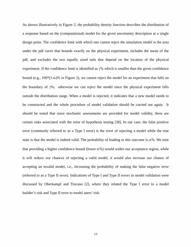
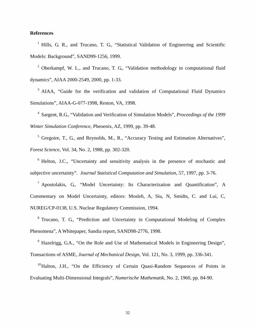
and compared with the results from physical tests. Provided in Figure 3 is an illustrative example
of model validation for a problem with two physical tests (corresponding to two design settings).
The joint pdf of y1 and y2 is first obtained for the same response, and then the boundary with 1-α
confidence level is determined by the iso-count contour that contains 100(1-α)% samples of
Monte Carlo Simulations conducted over the RSM. Theoretically, if the experimental result Y in
an n-dimensional space (n = 2 in this example) falls within the boundary, it indicates that we
cannot reject the model with a confidence level of (1-α). If the point falls outside of the
boundary, then we can reject the model with a confidence level of (1-α). Note the results of
single experiments at multiple design settings now become a single point in the multivariate
histogram space (see Figure 3).
Insert Figure 3. Model validation at two design settings
For multivariate distributions symmetric about their means, contours of constant probability are
given by ellipses determined with r2. r2, which can be thought of as a square of the weighted
distance of the physical experiments from the multivariate mean, can be related to normal
probability through the chi-square distribution for 100*(1-α)% confidence with n degrees of
freedom (n design settings). The prediction model can be rejected at 100*(1-α)% if the

15
combination of multiple design points measured from physical experiments is outside of 100*(1-
α)% confidence region.
According to Hills, a constant probability is given by the following ellipses where r2 is constant
for iso-probability curves.
[ ]⎥⎥⎥⎥
⎦
⎤
⎢⎢⎢⎢
⎣
⎡
−
−−
−−−−=
meannyny
meanyymeanyy
Vmeannynymeanyymeanyyr......
2211
1.....22112
(3)
In equation (3), yi, i = 1...n, stands for the single experimental result for each design setting i.
ymeani is the mean of the random samples obtained from the computer model at each testing point
i. The V matrix is the n by n co-variance matrix based on the random samples.
For model validation, the critical value of r2 is obtained as:
)(122 nlcriticalr α−= , (4)
where l is the value associated with the 100*(1-α)% confidence for n testing points through the
chi-square distribution. If the value of r2 from equation (3) is less than the critical value of r2
from equation (4), then we do not possess statistically significant evidence to declare our model
invalid, and vice versa. When an acceptable error region is considered (see the box shown in
Figure 3), the value of r2 is calculated based on the location of the extreme corner of the box.
16
3.4 Data Transformations for Model Validation Purposes
As stated earlier, the strategies for model validation introduced in Hills and Trucano [1] are
followed in this research. For comparison purposes, a test statistic r2 is employed in this research.
To apply the r2 criterion for model validation, the assumption of normality of the multivariate
joint probability distributions has to be satisfied.
Multivariate normality is the assumption that all dimensions and all combinations of the
dimensions are normally distributed. When the assumption is met, the residuals (differences
between predicted and obtained response values), are symmetrically distributed around a mean
of zero and follows a normal distribution. The assumption of normality often leads to tests that
are simple, mathematically tractable, and powerful compared to tests that do not make the
normality assumption.
The two methods for normality screening are the statistical approach and the graphical approach.
The statistical method employs examinations of significance for skewness and kurtosis. Mardia
[39] suggested useful measures of skewness and kurtosis. Skewness is related to the symmetry of
the distribution, while kurtosis is related to the peakedness of a distribution, either too peaked or
too flat. The graphical method visually assesses the distributions of the data and compares them
to the normal distribution.
Transformations can be applied to both the response (model output) and predictor (model input)
variables following the approaches discussed in Section 2.4. Only after employing
17
transformations can we apply the model validation procedure described earlier in Section 3.
RSM, MCS and equations (3) and (4) are applied for the transformed model to assess the model
validity.
3.5 Measurement error, response surface model error, and acceptable level of error
In the proposed model validation procedure, it is also important to consider various uncertainties
(errors) that cannot be predicted by the uncertainty propagation based on the computational
model. These errors include the measurement errors, the response surface model error, and the
acceptable level of error. To simplify the process, we count the measurement errors and response
surface model error by including them directly to the prediction uncertainty obtained through
uncertainty propagation. Specifying an acceptable level of error is practically significant because
the discrepancy between the simulated and experimental results indicates the errors associated
with the model structure and numerical procedures (Types II and III uncertainties discussed in
section 2). Approximated models should not be declared invalid if they provide predictions
within an error that the user finds acceptable for a particular application. The acceptable level of
error of a modeling approach is modeled as a box or a circle around the physical test point in
Figure 3. Figure 3 shows a situation in which the confidence region of the model prediction and
the acceptable error region overlap. This indicates that we cannot declare that the model is
invalid for the given confidence level considering the acceptable level of error.
4. VALIDATING A FINITE-ELEMENT MODEL OF SHEET METAL FLANGING
PROCESS
4.1 Sheet Metal Flanging Process and its Modeling
18
Sheet metal forming is one of the dominant processes in the manufacture of automobiles,
aircraft, appliances, and many other products. As one of the most common processes for
deforming sheet metals, flanging is used to bend an edge of a part to increase the stiffness of a
sheet panel and (or) to create a mating surface for subsequent assemblies. As the tooling is
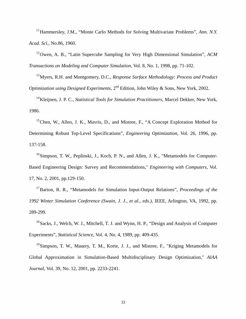
retracted, the elastic strain energy stored in the material recovers to reach a new equilibrium and
causes a geometric distortion due to elastic recovery (see Figure 4), the so-called “springback”
[40]. Springback refers to the shape discrepancy between the fully loaded and unloaded
configurations as shown in Figure 4.
Springback depends on a complex interaction between material properties, part geometry, die
design, and processing parameters. The capability to model and simulate the springback
phenomenon early in the new product design process can significantly reduce the product
development cycle and costs. However, many factors influence the amount of springback in a
physical test. Prediction and experimental testing of springback is particularly sensitive to the
various types of uncertainties as discussed in [41], [42]. Referring to the definitions of the three
types of uncertainties described in Section 2.1, examples of Type I uncertainty are the parameters
related to incoming sheet metal material, initial geometry, and process setup. An example of
Type II uncertainty is that, in material characterization, the hardening law to describe the
behavior of sheet metal under loading and reverse loading is often uncertain; Example of Type
III uncertainty is the numerical error caused by using different finite element analysis methods
for spring back angle estimation, e.g., implicit Finite Element Method, explicit Finite Element
Method, etc.
19
Insert Figure 4. Schematic of the springback in flanging
Various modeling approaches have been used to model the flanging process. These models
include both analytical models and finite element analysis-based models. In this study, we
illustrate how the proposed model validation approach can be applied to validate two finite
element analysis models that model the blank plasticity with the combined hardening (Model 1)
and isotropic hardening (Model 2) laws [43], respectively. The process is modeled by using an
implicit and static nonlinear finite element code, ABAQUS/standard (v.5.8.). The two models
with combined hardening and isotropic hardening laws are used to illustrate the effect of the fact
when the data from MCS follow either normal or a non-normal distribution. Normalizing
transformations are applied to the data from the model with the isotropic hardening law for
model validation procedure. The angle at the fully unloaded configuration (see Figure 4) is
considered as the process output (the response).
4.2 Problem Setup, Experiments, and Uncertainty Propagation in Validating Sheet Metal
Forming Process Models
We illustrate in this section how the major phases in the proposed model validation approach are
followed for our case study.
Phase I – Problem Setup
To accomplish Phase I, design variables and design parameters that affect the process output
(final flange angle θf) are determined. Primarily, two design variables that are related to the
process setup are considered, i.e. flange length, L; and gap space, g; and design parameters that
are related to the material are selected, i.e. sheet thickness, t; and material properties (namely,
Young’s Modulus, E; Strain Hardening Coefficient, n; Material Strength Coefficient, K; and

20
Yield Stress, Y) (see Figure 5). Design parameters are uncontrollable (given) while design
variables can be controlled over the design space to achieve the desired process output.
Insert Figure 5. System Diagram for Flanging Process
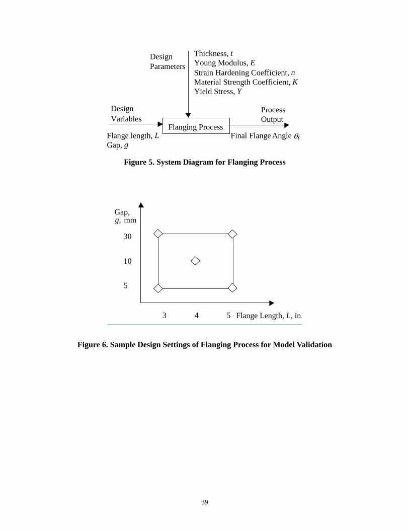
To form sample design settings, different combinations of values of design variables, i.e., L and
g, are used. Five sample design settings are formed with combinations of low and high levels of
flange length (3 and 5 inches) and gap (5 and 30 mm) plus a design point close to the middle (4
inches, 10 mm) (see Figure 6). These values for low, middle and high levels of flange length and
gap are selected so that they can cover the whole design space as uniformly as possible.
Insert Figure 6. Sample Design Settings of Flanging Process for Model Validation
The variations of design variables and design parameters are identified in this phase. Based on
experimental data, obtained by tensile tests, the relationships among K, n, and Y for carbon steel
sheet metals used in the tests are approximated as
97.4995.1128)( += nnK , and (5)
85.4848.779)( +−= nnY . (6)
Therefore, among the four parameters describing the material property, two are independent
parameters (n and E), and the other two (K and Y) are dependent. Also, the statistical
descriptions for these material parameters are obtained. The distribution of Young’s Modulus (E)
is assumed to be a normal distribution with 197949.7 MPa and 12914.7 MPa as the mean and
standard deviation, respectively. The distribution of strain-hardening exponent (n) is assumed to
be a uniform distribution from 0.10 to 0.18. The distributions of the strength coefficient (K) and
yield stress (Y) depend on n as shown in equations 3 and 4. The distribution of sheet thickness (t)
21
is assumed to be a normal distribution with 1.5529 mm and 0.0190 mm as the mean and standard
deviation, respectively. Similarly, the variation of the design variable gap space (g) is assumed to
be normally distributed with a standard deviation of 0.6 mm; note that the mean of the gap will
change based on the location of the design point. The variation of flange length (L) is ignored as
the flanging accuracy tolerance is insignificant comparing to the effect of the other change on
final flange angle.
Phase II – Experiments and Measurements
In this phase, physical experiments are conducted and measurement errors are estimated. The
dimensions of the sheet blank used in the physical experiments are 203.2 mm. x 203.2 mm. (or 8
inches x 8 inches). The flanging process uses a punch, a binder, a draw die, and a blank. The
experiments have been performed by the 150-ton computer controlled HPM hydraulic press in
the Advanced Materials Processing Laboratory at Northwestern University. The unloaded
configurations, i.e., the angles between two planes in degrees (see Figure 4), have been measured
by a coordinate measuring machine (Brown & Sharpe MicroVal Series Coordinate Measuring
Machine B89) in the metrology laboratory at Northwestern University.
Phase III – Model Simulation and Uncertainty Propagation
The flanging process has been numerically simulated based on two finite element models,
namely, one uses the combined hardening law (model 1) to the sheet material and model 2 uses
the isotropic hardening law.
22
The process has been modeled by an implicit and static nonlinear commercial finite element
code, ABAQUS/Standard. 1440 of eight-node, two-dimensional (plane strain) continuum
elements with reduced integration have been used in this problem to model the sheet blank
(ABAQUS element type CPE8R). The sheet thickness has been modeled with six layers. Tools
have been modeled as rigid surfaces. The coefficient of friction is set to 0.125. The interface
between the tooling and the sheet has been modeled by interface elements (IRS22) while the
penalty-based contact algorithm has been used. To have a better convergence rate, the surface
interaction is modeled by a soft contact. The analysis is performed in six steps: moving the
binder toward the blank; developing the binder force; moving the punch down to flange the
blank; retracting the punch up; releasing the binder force, and finally, moving the binder up.
The following two cases are considered in the simulation experiments for creating the response
surface models for model validation. The procedure is illustrated here only with Model 1
(combined hardening law). A similar procedure is followed in validating Model 2 (isotropic
hardening law).
Case 1: Validation at a single design point. 81 simulation experiments have been conducted to
create a response surface model for model validation at a single design point (3, 30), i.e., flange
length at 3 inches and gap at 30 mm. The response surface model represents the springback angle
as a function across over a range of design parameters (g, t, E, n, K, Y) corresponding to a single
design setting of L =3 inches. The 81 simulation experiments are designed based on various
combinations of (g, t, E, n, K, Y), where three levels are considered for both gap (g – 25, 30 and
35 inches at each level) and thickness (t – 1.483, 1.545 and 1.608 mm at each level) and a full
23
factorial design of these two factors are combined with nine settings of (E, n, K, Y) that capture a
wide range of the material property.
Case 2: Validation for multiple design settings. 243 simulation experiments have been conducted
to create the response surface model for model validation at five design points, i.e., the following
combinations of design variables (flange length in inches, and gap in millimeters): (3, 5), (3, 30),
(4, 10), (5, 30) and (5, 5). The response surface model represents the final flange angle as a
function of (L, g, t, E, n, K, Y). The 243 simulation experiments are designed based on various
combinations of (L, g, t, E, n, K, Y). Similar to the strategy used for designing the experiments in
Case 2, three levels are considered for flange length (L), gap (g), and thickness (t) and a full
factorial design of these three factors are combined with nine settings of (E, n, K, Y) that capture
a wide range of the material property.
The second order Polynomial Regression (PR) approximation models are first used to create
response surface models for both Cases 1 and 2. The accuracy is assessed by examining the sum
of squares of error (SSE) based on a set of confirmation tests. For Model 1, the results are
obtained as: SSE for PR is 0.0212 for Case 1 and SSE for PR is 0.9862 for 2. Considering that
the magnitude of the angle of the final configuration is in the range of 100 to 150 degrees, the
achieved SSE from PR is quite satisfactory. Therefore, for uncertainty propagation and model
validation, the results from the polynomial models will be used.
Once the response surface models are created, the MCS has been used to efficiently predict the
distributions of the final flange angle under uncertainty using 200,000 random sample points.
24
The uncertainty descriptions identified in Phase I, are followed for random sampling. The
predicted distributions of the final flange angle will be presented together with the validity
results next.
Phase IV – Model Validation via Comparisons
Normality Check
To simplify the model validation process, the predicted distributions of the final flange angle (for
single design point and each individual design point in multiple design settings) have been
checked for normality. The resulting probability distributions from Model 1 are plotted in Figure
7 (Case 1) and Figure 8 (Case 2).
Insert Figure 7. Confidence Limits based on Polynomial Model at Single Design Point
In Figures 7 and 8, the light pdf curve is the fitted normal distribution. It is noted that in general,
the predictions (considered separately for each design point) based on polynomial models are all
very close to normal. Kolmogorov-Smirnov (K-S) Test [44] has been conducted for normality
check. Following the procedures in the literature, the sample size for K-S test is determined to be
N=1000 (see [44], page 431). 1000 samples are randomly selected from the 200,000 simulations.
If the K-S statistic obtained from a K-S test is greater than the critical value, here 0.043 for
N=1000, the test rejects the Null Hypothesis (which states that the sample is drawn from a
normal distribution). The K-S statistic is obtained as 0.04 for Case 1, which means we cannot
reject the Null Hypothesis at α=0.05, and therefore the distribution can be considered as normal.
The normality assumption can greatly simplify the validation process, which is introduced next.
Validation of Model 1 (Combined hardening law)
Case 1: For the single design point (3, 30), the results of the predicted springback angles based
on MCS using the response surface model are compared with the result from a single physical
25
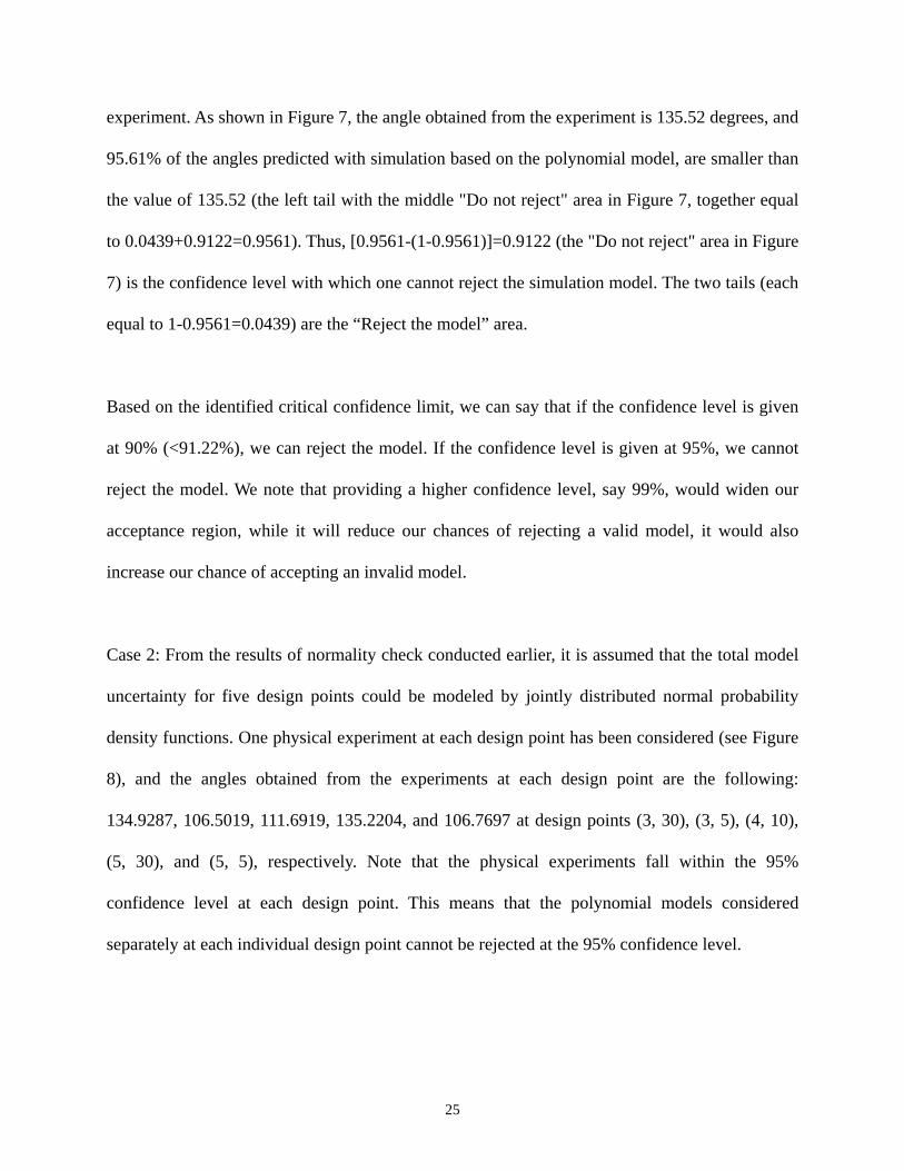
experiment. As shown in Figure 7, the angle obtained from the experiment is 135.52 degrees, and
95.61% of the angles predicted with simulation based on the polynomial model, are smaller than
the value of 135.52 (the left tail with the middle "Do not reject" area in Figure 7, together equal
to 0.0439+0.9122=0.9561). Thus, [0.9561-(1-0.9561)]=0.9122 (the "Do not reject" area in Figure
7) is the confidence level with which one cannot reject the simulation model. The two tails (each
equal to 1-0.9561=0.0439) are the “Reject the model” area.
Based on the identified critical confidence limit, we can say that if the confidence level is given
at 90% (<91.22%), we can reject the model. If the confidence level is given at 95%, we cannot
reject the model. We note that providing a higher confidence level, say 99%, would widen our
acceptance region, while it will reduce our chances of rejecting a valid model, it would also
increase our chance of accepting an invalid model.
Case 2: From the results of normality check conducted earlier, it is assumed that the total model
uncertainty for five design points could be modeled by jointly distributed normal probability
density functions. One physical experiment at each design point has been considered (see Figure
8), and the angles obtained from the experiments at each design point are the following:
134.9287, 106.5019, 111.6919, 135.2204, and 106.7697 at design points (3, 30), (3, 5), (4, 10),
(5, 30), and (5, 5), respectively. Note that the physical experiments fall within the 95%
confidence level at each design point. This means that the polynomial models considered
separately at each individual design point cannot be rejected at the 95% confidence level.

26
Equations 3 and 4 have been used to calculate r2 for the polynomial model. r2 for the polynomial
model is 7.4462 for Model 1. For the 95% confidence level, the critical value of r2 is obtained as
07.11)5(2%95
2 == lrcritical (7)
Since the r2 from the polynomial model is smaller than the critical r2, there is not enough
statistical evidence to conclude that the polynomial model is not valid. We find that for the
polynomial model, the critical confidence limit (p-value) lies on about 80% contour because r2
for 80%, for 5 dof = 7.289.
Insert Figure 8. Pdf Plots for Multiple Design Points, Model 1
Validation of Model 2 (Isotropic hardening law).
The validation of Model 2 is only illustrated for Case 2, i.e., for multiple design points, to
demonstrate how data transformations can be applied to non-normal response distributions. The
total model uncertainty for five design points again, has been modeled by jointly distributed
normal probability density functions and one physical experiment at each design point has been
considered. It is found that the response distributions obtained through the response surface
models are non-normal at each design point. One can see in Figure 9 that the original distribution
is right skewed with the right tail longer than the left tail. The null hypothesis for Kolmogorov-
Smirnov test is rejected at α=0.05, and the KS statistic is 0.05 with P-value of P = 2.9408e-04.
Plots of the probability density functions and the results of K-S tests at the other design points
are similar to those provided for design point (3,30).
Insert Figure 9. Pdf Plot for Multiple Design Points, Model 2
27
Data transformations are applied to represent the distributions in scales that are close to normal.
Unfortunately, the transformations (for response only) obtained by following the existing data
transformation techniques (see Section 2.4) are not satisfactory because for this problem the ratio
of the largest to the smallest observation is very close to one, a condition under which the
existing techniques are not applicable. We then decide to apply transformations to both the
response and the independent variables (model inputs) to overcome this difficulty. After some
tests, it is found that when applying natural log transformations (λ=0) to both dependent (i.e., the
angle at the unloaded configuration) and all independent variables (i.e., the design variables and
parameters) from FEA model, the transformed distributions can be considered as normal. A
polynomial response surface model is constructed using the transformed values of 243
observations from FEA at each design point (see Equation 8).
∑∑ ++=ji
jiiji
ii xxcXbaZ,
lnlnlnln (8)
These response surface models are used to predict the values of transformed dependent variables
and to obtain their distributions at all design points. The SSE=0.00282179 for the new
polynomial model in Equation 8 shows that the transformed model is quite accurate. The
normality check and model validation for 200,000 sample points at each design setting are
carried out for the obtained transformed model.
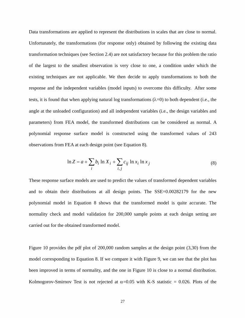
Figure 10 provides the pdf plot of 200,000 random samples at the design point (3,30) from the
model corresponding to Equation 8. If we compare it with Figure 9, we can see that the plot has
been improved in terms of normality, and the one in Figure 10 is close to a normal distribution.
Kolmogorov-Smirnov Test is not rejected at α=0.05 with K-S statistic = 0.026. Plots of the
28
probability density functions and the results of K-S tests for the other design points are similar to
those provided for design point (3,30). The K-S statistics are 0.027, 0.029, 0.024 and 0.032 for
the design points (3, 5), (4, 10), (5, 30) and (5, 5), respectively. Note that all of the values are
smaller than the critical K-S statistic, i.e. 0.043. This indicates that the transformations to
normal distributions are satisfactory.
Insert Figure 10. Transformed Pdf Plot, Model 2
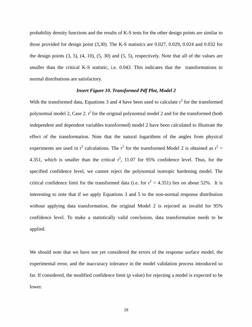
With the transformed data, Equations 3 and 4 have been used to calculate r2 for the transformed
polynomial model 2, Case 2. r2 for the original polynomial model 2 and for the transformed (both
independent and dependent variables transformed) model 2 have been calculated to illustrate the
effect of the transformation. Note that the natural logarithms of the angles from physical
experiments are used in r2 calculations. The r2 for the transformed Model 2 is obtained as r2 =
4.351, which is smaller than the critical r2, 11.07 for 95% confidence level. Thus, for the
specified confidence level, we cannot reject the polynomial isotropic hardening model. The
critical confidence limit for the transformed data (i.e. for r2 = 4.351) lies on about 52%. It is
interesting to note that if we apply Equations 3 and 5 to the non-normal response distribution
without applying data transformation, the original Model 2 is rejected as invalid for 95%
confidence level. To make a statistically valid conclusion, data transformation needs to be
applied.
We should note that we have not yet considered the errors of the response surface model, the
experimental error, and the inaccuracy tolerance in the model validation process introduced so
far. If considered, the modified confidence limit (p value) for rejecting a model is expected to be
lower.
29
4.3 Measurement, Response Surface Model Errors, and Acceptable Level of Error
Following the statistical description in Section, the measurement error and the response surface
model error are added directly to the predicted values of springback angle using MCS samples.
The procedure is demonstrated here only for Model 1.
The mean and the variance of the response surface model error are estimated as the mean and the
variance of the differences between the angles obtained from the FEM simulation and those
predicted with the response surface model for 200 samples. The samples are obtained with
Optimum Latin Hypercube Sampling (OLHS) [45]. As the result, the normal distribution N (-
0.7120776, 0.605479) is used to describe the error of the polynomial model in Case 1, and N (-
0.6311915, 1.0657299) is used to describe the error of the polynomial model in Case 2.
The mean and the variance of the measurement error are obtained based on the specification of
the CMM machine, represented as N (0, 0.04193576). Simulation is used to obtain samples from
normal distributions with the corresponding parameters as described above for the response
surface model error and the measurement error.
The simulated errors are added observation-by-observation to the samples of springback angle
from MCS for Case 1 and Case 2. Thus, new distributions that incorporate the errors are
obtained for each case. The acceptable level of error is set to ±0.5 degree and incorporated by
adjusting the result from the physical experiment. Thus, for the value of 135.52 (degrees)
obtained from the physical experiment, the model cannot be rejected if the response distribution

30
falls to the left of the minimum acceptable value of the experiment, i.e. 135.52 - 0.5 = 135.02
(degrees) (see Figure 11). In Figure 11, the curve with upper tails and lower pick reflects the
modified pdf, which is checked against the lower limit of acceptable error range. Note that
considering different errors reduces the possibility of rejecting a model.
Insert Figure 11. Considering Various Types of Errors
Case 1: Single design point: the confidence limit for 135.02 (degrees) is 87.95% for the
polynomial model after the modification.
Case 2: Multiple design settings: r2 for the polynomial model is 3.67 for the minimum acceptable
values of the experiments for all design points, i.e., 134.4287, 106.0019, 111.1919, 134.7204,
and 106.2697. As mentioned earlier, for the 95% confidence level, the critical value of r2 is
11.07. Thus, the polynomial model for multiple design points cannot be rejected at 95%
confidence level. The critical limit for the polynomial model lies on about 40% since r2 for 40%,
for 5 dof = 3.6555.
5. CONCLUSIONS
In this paper an approach for model validation via uncertainty propagation using the response
surface methodology is presented. The approach uses response surface methodology to create
metamodels as less costly approximations of simulation models for uncertainty propagation. Our
proposed model validation procedure incorporates various types of uncertainties involved in a
model validation process and significantly reduces the amount of physical experiments. The
proposed approach can be used to provide stochastic assessment of model validity across a
design space instead of a single point. The approach has been illustrated with an example of a
sheet metal flanging process, for two finite element models (FEM) based on the combined

31
hardening law and the isotropic hardening law, respectively. For the FEM model based on the
combined hardening law, polynomial response surface models are created for both cases and
confirmed to be accurate; they are used for uncertainty propagation in both cases. The critical
confidence levels are identified by comparing the performance distribution obtained from
uncertainty propagation with the results from the single experiments. The polynomial models
have not been statistically declared as invalid if the given significant level is set at 95% for both
single and multiple design points. The results are adjusted after considering the response surface
model error, the measurement error, and the acceptable level of error.
For the FEM model based on the isotropic hardening law, the response distribution does not
follow the normal distribution. The approach suggests to employ data transformations to the
polynomial model based on isotropic hardening law. For the tested finite element model based on
the combined hardening law, the model cannot be statistically declared as invalid if the given
significant level is set at 95% for both single and multiple design points.
Future research will be directed toward integrating the model validation approach as a part of the
model selection and decision making in engineering design.
Acknowledgments
The support from the National Science Foundation for the project "Collaborative Research: An
Approach for Model Validation in Simulating Sheet Metal Forming Processes", by the Civil and
Mechanical Systems Division (CMS0084477 for University of Illinois at Chicago; CMS-
0084582 for Northwestern University), is greatly appreciated.
32
References
1 Hills, G. R., and Trucano, T. G., “Statistical Validation of Engineering and Scientific
Models: Background”, SAND99-1256, 1999.
2 Oberkampf, W. L., and Trucano, T. G., “Validation methodology in computational fluid
dynamics”, AIAA 2000-2549, 2000, pp. 1-33.
3 AIAA, “Guide for the verification and validation of Computational Fluid Dynamics
Simulations”, AIAA-G-077-1998, Reston, VA, 1998.
4 Sargent, R.G., “Validation and Verification of Simulation Models”, Proceedings of the 1999
Winter Simulation Conference, Pheoenix, AZ, 1999, pp. 39-48.
5 Gregoire, T., G., and Reynolds, M., R., “Accuracy Testing and Estimation Alternatives”,
Forest Science, Vol. 34, No. 2, 1988, pp. 302-320.
6 Helton, J.C., “Uncertainty and sensitivity analysis in the presence of stochastic and
subjective uncertainty”. Journal Statistical Computation and Simulation, 57, 1997, pp. 3-76.
7 Apostolakis, G., “Model Uncertainty: Its Characterization and Quantification”, A
Commentary on Model Uncertainty, editors: Mosleh, A, Siu, N, Smidts, C. and Lui, C,
NUREG/CP-0138, U.S. Nuclear Regulatory Commission, 1994.
8 Trucano, T. G., “Prediction and Uncertainty in Computational Modeling of Complex
Phenomena”, A Whitepaper, Sandia report, SAND98-2776, 1998.
9 Hazelrigg, G.A., “On the Role and Use of Mathematical Models in Engineering Design”,
Transactions of ASME, Journal of Mechanical Design, Vol. 121, No. 3, 1999, pp. 336-341.
10 Halton, J.H., “On the Efficiency of Certain Quasi-Random Sequences of Points in
Evaluating Multi-Dimensional Integrals”, Numerische Mathematik, No. 2, 1960, pp. 84-90.
33
11 Hammersley, J.M., “Monte Carlo Methods for Solving Multivariate Problems”, Ann. N.Y.
Acad. Sci., No.86, 1960.
12 Owen, A. B., “Latin Supercube Sampling for Very High Dimensional Simulation”, ACM
Transactions on Modeling and Computer Simulation, Vol. 8, No. 1, 1998, pp. 71-102.
13 Myers, R.H. and Montgomery, D.C., Response Surface Methodology: Process and Product
Optimization using Designed Experiments, 2nd Edition, John Wiley & Sons, New York, 2002.
14 Kleijnen, J. P. C., Statistical Tools for Simulation Practitioners, Marcel Dekker, New York,
1986.
15 Chen, W., Allen, J. K., Mavris, D., and Mistree, F., “A Concept Exploration Method for
Determining Robust Top-Level Specifications”, Engineering Optimization, Vol. 26, 1996, pp.
137-158.
16 Simpson, T. W., Peplinski, J., Koch, P. N., and Allen, J. K., "Metamodels for Computer-
Based Engineering Design: Survey and Recommendations," Engineering with Computers, Vol.
17, No. 2, 2001, pp.129-150.
17 Barton, R. R., “Metamodels for Simulation Input-Output Relations”, Proceedings of the
1992 Winter Simulation Conference (Swain, J. J., et al., eds.), IEEE, Arlington, VA, 1992, pp.
289-299.
18 Sacks, J., Welch, W. J., Mitchell, T. J. and Wynn, H. P., “Design and Analysis of Computer
Experiments”, Statistical Science, Vol. 4, No. 4, 1989, pp. 409-435.
19 Simpson, T. W., Mauery, T. M., Korte, J. J., and Mistree, F., "Kriging Metamodels for
Global Approximation in Simulation-Based Multidisciplinary Design Optimization," AIAA
Journal, Vol. 39, No. 12, 2001, pp. 2233-2241.

34
20 Meckesheimer, M., Barton, R. R., Limayem, F., and Yannou, B., “Metamodeling of
Combined Discrete/Continuous Responses”, Design Theory and Methodology – DTM’00 (Allen,
J.K., Ed.), ASME, Baltimore, MD, 2000, Paper No. DETC2000/DTM-14573.
21 Jin, R, Chen, W., and Simpson T., “Comparative Studies of Metamodeling Techniques
under Multiple Modeling Criteria”, Journal of Structural & Multidisciplinary Optimization, Vol.
23, No. 1, 2001, pp. 1-13.
22 Jin, R., Du, X, and Chen, W., “The Use of Metamodeling Techniques for Optimization
under Uncertainty”, 2001 ASME Design Automation Conference, Pittsburgh, PA, 2001, Paper
No. DAC21039, in press, Journal of Structural & Multidisciplinary Optimization.
23 Bartlet, M. S., “The Use of Transformations”, Biometrics, Vol. 3, No. 1, 1947, pp. 39-52.
24 Tukey, J. W., “On the Comparative Anatomy of Transformations”, Annals of Mathematical
Statistics, Vol. 28, No. 3, 1957, pp. 602-632.
25 Box, G. E. P., and Cox, D. R., “An Analysis of Transformations”, Journal of the Royal
Statistical Society B, Vol. 26, No. 2, 1964, pp. 211-252.
26 Hinkley, D., “ On Quick Choice of Power Transformation”, Applied Statistics, Vol. 26, No.
1, 1977, pp. 67-69.
27 Manly, B. F. J., “Exponential data transformations”, Statistician, Vol. 25, No. 1, 1976, pp.
37-42.
28 John, J. A., and Draper, N. R., “An Alternative Family of Transformations”, Applied
Statistics, Vol. 29, No. 2, 1980, pp. 190-197.
29 Yeo, In-Kwon and Johnson, R., “A New Family of Power Transformations to Improve
Normality or Symmetry”, Biometrika, Vol. 87, 2000, pp. 954-959.
35
30 Atkinson, A. C., “Testing Transformations to Normality”, Journal of the Royal Statistical
Society B, Vol. 35, No. 3, 1973, pp. 473-479.
31 Carroll, R. J. “A Robust Method for Testing Transformations to Achieve Approximate
Normality”, Journal of the Royal Statistical Society B, Vol. 42, No. 1, 1980, pp. 71-78.
32 Atkinson, A. C., and Riani, M., “Bivariate boxplots, multiple outliers, multivariate
transformations and discriminant analysis: the 1997 Hunter lecture”, Environmetrics, Vol. 8,
1997, pp. 583--602.
33 Krzanowski, W. J., Principles of Multivariate Analysis: A User’s Perspective, Clarendon
Press, Oxford, paperback edition, 1990.
34 Velilla, S., “Diagnostics and robust estimation in multivariate data transformations”,
Journal of the American Statistical Association, Vol. 90, No. 431, 1995, pp. 945--951.
35 Box, G. E. P., and Tidwell, P. W., “Transformation of the Independent Variables”,
Technometrics, Vol. 4, No. 4, 1962, pp. 531-550.
36 McKay, M.D., Beckman, R.J., and Conover, W.J., “A comparison of three methods for
selecting values of input variables in the analysis of output from a computer code”,
Technometrics, Vol. 21, No. 2, 1979, pp. 239-45.
37 Koehler, J.R. and Owen, A.B., “Computer experiments”, in Ghosh, S.and Rao, C.R., eds,
Handbook of Statistics, 13, 1996, 261 –308, Elsevier Science, New York.
38 Kleinbaum, D.G., Kupper, L.L., Muller, K.E., and Nizam, A., Applied Regression Analysis
and Other Multivariate Methods, 3rd Edition, Duxbury Press, CA, 1998.
39 Mardia, K. V., “Applications of Some Measures of Multivariate Skewness and Kurtosis for
Testing Normality and Robustness Studies”, Sankhya B, Vol. 36, 1974, pp. 115-128.

36
40 Song, N., Qian, D., Cao, J., Liu, W. K., and Li, S., “Effective Prediction of Springback in
Straight Flanging”, Journal of Engineering Materials and Technology, Vol. 123, No. 4, 2001, pp.
456-461.
41 Hu, Y., and Walters, G. N., “A Few Issues On Accuracy of Springback Simulation of
Automobile Parts”, SAE Paper No. 1999-01-1000, SAE SP-1435, 1999.
42 Esche, S., and Kinzel, G., “The Effect of Modeling Parameters and Bending on Two-
dimensional Sheet Metal Forming Simulation”, SAE Transactions, Vol. 107, No. 7, 1998, pp.74-
85.
43 ABAQUSTM: User’s Manual, Hibbit, Karlson, and Sorensen, Inc, RI.
44 Birnbaum, Z. W., “Numerical Tabulation of the Distribution of Kolmogorov’s Statistic for
Finite Sample Size”, Journal of the American Statistical Association, Vol. 47, No. 259, 1952, pp.
425-441.
45 Sudjianto, A., Juneja, L., Agrawal, H.v and Vora, M., “Computer aided Reliability and
robustness assessment”, International Journal of Reliability, Quality and Safety Engineering,
Vol. 5, No. 2, 1998, pp. 181-193.

37
Define an Acceptable Level of Error
Identify Sources of Variations Sample Design Settings
Phase I: Problem Setup Phase IV:
Model Validation Via Comparisons
Phase III: Model Uncertainty Propagation
Employ Efficient Uncertainty Propagation Scheme
Analytical Model or Numerical Simulation
Calculate Multivariate Probabilistic Distributions
Experiments andMeasurements
Estimate Measurements Error
Phase II: Experiments Forming Exps atDifferent DesignSettings
Figure 1. Procedure for Model Validation
Confidence Limit Physical Experiment
0
0.05
0.1
0.15
0.2
0.25
0.3
0.35
0.4 probability
100*(1 - α )% Confidence Bound
100* γ %
response
Figure 2. Model Validation for a Single Design Point
38
5.5 6 6.5 7 7.5 8 8.5 9 9.5 10
11
12
13
14
15
16
y1
y 2
100*(1-α)% confidence boundary
Acceptable error region
Experiment
Figure 3. Model validation at two design settings
g
Binder
DieθO
θf
Punch
∆θ
L
Figure 4. Schematic of the springback in flanging; g is the gap between the die and the punch,
θ0 is the flange angle at the fully loaded configuration, θf is that of the unloaded configuration,
and ∆θ is the springback.
39
Flanging Process
Design Variables
Flange length, L Gap, g
Process Output
Final Flange Angle θf
Design Parameters
Thickness, t Young Modulus, E Strain Hardening Coefficient, n Material Strength Coefficient, K Yield Stress, Y
Figure 5. System Diagram for Flanging Process
Gap, g, mm
3 4 5
30
10
5
Flange Length, L, in.
Figure 6. Sample Design Settings of Flanging Process for Model Validation

40
ConfidenceLimit
Physical Experiment
= 135.52
130 131 132 133 134 135 136 137 138 0 0.05 0.1
0.15 0.2
0.25
0.3 0.35 0.4
angle at the unloaded configuration (degree)
probability “Do Not Reject” = 91.22%
1-0.9561 = 0.0439
0.0439
Figure 7. Confidence Limits based on Polynomial Model at Single Design Point (3, 30),
Model 1. The Light curve is the pdf of fitted normal distribution

41
130 131 132 133 134 135 136 137 1380
0.05
0.1
0.15
0.2
0.25
0.3
0.35
0.4
0.45The probability density function at (3,30)
angle at the unloaded configuration (degree)
prob
abili
ty
(a)
109 110 111 112 113 114 115 116 117 1180
0.05
0.1
0.15
0.2
0.25
0.3
0.35
0.4The probability density function at (4,10)
angle at the unloaded configuration (degree)
prob
abili
ty
(c)
102 103 104 105 106 107 10 8 109 1100
0.05
0.1
0.15
0.2
0.25
0.3
0.35
0.4The probability density function at (5,5)
angle at the unloaded configuration (degree)
prob
abili
ty
(e)
102 103 104 105 106 107 10 8 109 1100
0.05
0.1
0.15
0.2
0.25
0.3
0.35
0.4The probability density function at (3,5)
angle at the unloaded configuration (degree)
prob
abili
ty
(b)
130 131 132 133 134 135 13 6 137 1380
0.05
0.1
0.15
0.2
0.25
0.3
0.35
0.4
0.45The probability density function at (5,30)
angle at the unloaded configuration (degree)
prob
abili
ty
(d)
Figure 8. Pdf Plots for Multiple Design
Points, Model 1; polynomial model at
design points: (a) (3,30), (b) (3,5), (c) (4,
10), (d) (5,30), and (e) (5, 5). The light pdf
curve is the fitted normal distribution at each
design point. The two vertical lines are 95%
confidence level and the line between them
is the angle obtained from physical
experiment at each design point.

42
Figure 9. Pdf Plot for Multiple Design Points, Model 2; Polynomial model at design point
(3,30). The light pdf curve is the fitted normal distribution.
Figure 10. Transformed Pdf Plot, Model 2; after transforming the independent variable and the
dependent variables, λ=0, at design point (3, 30). The light curve is the fitted normal distribution.

43
130 131 132 133 134 135 136 137 138 0
0.05
0.1
0.15
0.2
0.25
0.3
0.35
0.4
Angle at the unloaded configuration (degree)
probability
95% Confidence Bound
Physical Experiment
Acceptable error range
ResponseSurface
Model Error &Experiment MeasurementError
Figure 11. Considering Various Types of Errors


