
Modeling of Supply Chain Risk Under Disruptions with
Performance Measurement and Robustness Analysis
Qiang Qiang and Anna Nagurney
Department of Finance and Operations Management
Isenberg School of Management
University of Massachusetts
Amherst, Massachusetts 01003
June Dong
Department of Marketing and Management
School of Business
State University of New York at Oswego
Oswego, New York 13126
June 2008; appears in slightly revised form in:
Managing Supply Chain Risk and Vulnerability:
Tools and Methods for Supply Chain Decision Makers
T. Wu and J. Blackhurst, Editors, Springer, Berlin, Germany, 2009, pp. 91-111.
Abstract: In this paper, we develop a new supply chain network model with multiple
decision-makers associated at different tiers and with multiple transportation modes
for shipment of the good between tiers. The model formulation captures supply-
side risk as well as demand-side risk, along with uncertainty in transportation and
other costs. The model also incorporates the individual attitudes towards disruption
risks among the manufacturers and the retailers, with the demands for the product
associated with the retailers being random. We present the behavior of the various
decision-makers, derive the governing equilibrium conditions, and establish the finite-
dimensional variational inequality formulation. We also propose a weighted supply
chain performance and robustness measure based on our recently derived network
performance/efficiency measure and provide supply chain examples for which the
equilibrium solutions are determined along with the robustness analyses. This paper
extends previous supply chain research by capturing supply-side disruption risks,
transportation and other cost risks, and demand-side uncertainty within an integrated
modeling and robustness analysis framework.
1
1. Introduction
Supply chain disruptions and the associated risk are major topics in theoreti-
cal and applied research, as well as in practice, since risk in the context of sup-
ply chains may be associated with the production/procurement processes, the trans-
portation/shipment of the goods, and/or the demand markets. In fact, Craighead,
Blackhurst, Rungtusanatham, and Handfield (2007) have argued that supply chain
disruptions and the associated operational and financial risks are the most pressing
issue faced by firms in today’s competitive global environment. Notably, the focus
of research has been on “demand-side” risk, which is related to fluctuations in the
demand for products, as opposed to the “supply-side” risk, which deals with uncer-
tain conditions that affect the production and transportation processes of the supply
chain. For a discussion of the distinction between these two types of risk, see Snyder
(2003).
For example, several recent major disruptions and the associated impacts on the
business world have vividly demonstrated the need to address supply-side risk with
a case in point being a fire in the Phillips Semiconductor plant in Albuquerque,
New Mexico, causing its major customer, Ericsson, to lose $400 million in potential
revenues. On the other hand, another major customer, Nokia, managed to arrange
alternative supplies and, therefore, mitigated the impact of the disruption (cf. La-
tour (2001)). Another illustrative example concerns the impact of Hurricane Katrina,
with the consequence that 10% - 15% of total U.S. gasoline production was halted,
which not only raised the oil price in the U.S., but also overseas (see, e. g., Cana-
dian Competition Bureau (2006)). Moreover, the world price of coffee rose 22% after
Hurricane Mitch struck the Central American republics of Nicaragua, Guatemala,
and Honduras, which also affected supply chains worldwide (Fairtrade Foundation
(2002)). As summarized by Sheffi (2005) on page 74, one of the main characteris-
tics of disruptions in supply networks is “the seemingly unrelated consequences and
vulnerabilities stemming from global connectivity.” Indeed, supply chain disruptions
may have impacts that propagate not only locally but globally and, hence, a holistic,
system-wide approach to supply chain network modeling and analysis is essential in
order to be able to capture the complex interactions among decision-makers.
2

Indeed, rigorous modeling and analysis of supply chain networks, in the presence of
possible disruptions is imperative since disruptions may have lasting major financial
consequences. Hendricks and Singhal (2005) analyzed 800 instances of supply chain
disruptions experienced by firms whose stocks are publicly traded. They found that
the companies that suffered supply chain disruptions experienced share price returns
33 percent to 40 percent lower than the industry and the general market benchmarks.
Furthermore, share price volatility was 13.5 percent higher in these companies in
the year following a disruption than in the prior year. Based on their findings, it
is evident that only well-prepared companies can effectively cope with supply chain
disruptions. Wagner and Bode (2007), in turn, designed a survey to empirically study
the responses from executives of firms in Germany regarding their opinions as to the
factors that impact supply chain vulnerability. The authors found that demand-side
risks are related to customer dependence while supply-side risks are associated with
supplier dependence, single sourcing, and global sourcing.
The goal of supply chain risk management is to alleviate the consequences of
disruptions and risks or, simply put, to increase the robustness of a supply chain.
However, there are very few quantitative models for measuring supply chain robust-
ness. For example, Bundschuh, Klajan, and Thurston (2003) discussed the design of
a supply chain from both reliability and robustness perspectives. The authors built a
mixed integer programming supply chain model with constraints for reliability and ro-
bustness. The robustness constraint was formulated in an implicit form: by requiring
the suppliers’ sourcing limit to exceed a certain level. In this way, the model builds
redundancy into a supply chain. Snyder and Daskin (2005) examined supply chain
disruptions in the context of facility location. The objective of their model was to
select locations for warehouses and other facilities that minimize the transportation
costs to customers and, at the same time, account for possible closures of facilities
that would result in re-routing of the product. However, as commented in Snyder and
Shen (2006), “Although these are multi-location models, they focus primarily on the
local effects of disruptions.” Santoso, Ahmed, Goetschalckx, and Shapiro (2005) ap-
plied a sample average approximation scheme to study the stochastic facility location
problem by considering different disruption scenarios.
3
Tang (2006a) also discussed how to deploy certain strategies in order to enhance
the robustness and the resiliency of supply chains. Kleindorfer and Saad (2005), in
turn, provided an overview of strategies for mitigating supply chain disruption risks,
which were exemplified by a case study in a chemical product supply chain. For a
comprehensive review of supply chain risk management models to that date, please
refer to Tang (2006b).
To-date, however, most supply disruption studies have focused on a local point of
view, in the form of a single-supplier problem (see, e. g., Gupta (1996) and Parlar
(1997)) or a two-supplier problem (see, e. g., Parlar and Perry (1996)). Very few
papers have examined supply chain risk management in an environment with multi-
ple decision-makers and in the case of uncertain demands (cf. Tomlin (2006)). We
believe that it is imperative to study supply chain risk management from a holistic
point of view and to capture the interactions among the multiple decision-makers in
the various supply chain network tiers. Indeed, such a perspective has also been ar-
gued by Wu, Blackhurst, and Chidambaram (2006), who focused on inbound supply
risk analysis. Towards that end, in this paper, we take an entirely different per-
spective, and we consider, for the first time, supply chain robustness in the context
of multi-tiered supply chain networks with multiple decision-makers under equilib-
rium conditions. For a plethora of supply chain network equilibrium models and the
associated underlying dynamics, see the book by Nagurney (2006a).
Of course, in order to study supply chain robustness, an informative and effective
performance measure is first required. Beamon (1998, 1999) reviewed the supply chain
literature and suggested directions for research on supply chain performance measures,
which should include criteria on efficient resource allocation, output maximization,
and flexible adaptation to the environmental changes (see also, Lee and Whang (1999),
Lambert and Pohlen (2001), and Lai, Ngai, and Cheng (2002)). We emphasize that
different supply performance measures can be devised based on the specific nature of
the problem. In any event, the discussion here is not meant to cover all the existing
supply chain performance measures. Indeed, we are well aware that it is a daunting
task to propose a supply chain performance measure that covers all aspects of supply
chains. We believe that such a discussion will be an ongoing research topic for decades
4
to follow. In this paper, we study supply chain robustness based on a novel network
performance measure proposed by Qiang and Nagurney (2008), which captures the
network flows, the costs, and the decision-makers’ behavior under network equilibrium
conditions.
In particular, the model developed in this paper extends the supply chain model
of Nagurney, Dong, and Zhang (2002) with consideration of random demand (cf.
Nagurney, Cruz, Dong, and Zhang (2005)). In order to study supply chain robustness,
the new model contains the following novel features:
• We associate each process in a supply chain with random cost parameters to
represent the impact of disruptions to the supply chain.
• We extend the aforementioned supply chain models to capture the attitude of
the manufacturers and the retailers towards disruption risks.
• We propose a weighted performance measure to evaluate different supply chain
disruptions.
• Different transportation modes are considered in the model (see also, e.g., Dong,
Zhang, and Nagurney (2002) and Dong, Zhang, Yan, and Nagurney (2005)). In
the multimodal transportation supply chain, alternative transportation modes
can be used in the case of the failure of a transportation mode. Indeed, many
authors have emphasized that redundancy needs to be considered in the design
of supply chains in order to prevent supply chain disruptions. For example,
Wilson (2007) used a system dynamic simulation to study the relationship be-
tween transportation disruptions and supply chain performance. The author
found that the existence of transportation alternatives significantly improved
supply chain performance in the case of transportation disruptions.
In this paper, we assume that the probability distributions of the disruption re-
lated cost parameters are known. This assumption is not unreasonable given today’s
advanced information technology and increasing awareness of the risks among man-
agers. A great deal of disruption related information can be obtained from a careful
5

examination and abstraction of the relevant data sources. Specifically, as indicated
by Sheffi (2005) on page 55, “... as investigation boards and legal proceedings have
revealed, in many cases relevant data are on the record but not funneled into a useful
place or not analyzed to bring out the information in the data.” Moreover, Holmgren
(2007) also discussed ways to improve prediction of disruptions, using, for example:
historical data analysis, mathematical modeling, and expert judgments. Furthermore,
we assume that the random cost parameters are independent.
The organization of this paper is as follows. In Section 2, we present the model of
a supply chain network faced with (possible) disruptions and in the case of random
demands and multiple transportation modes. In Section 3, we provide a definition of
a weighted supply chain performance measure with consideration of robustness. In
Section 4, we present numerical examples in order to illustrate the model and concepts
introduced in this paper. The paper concludes with Section 5, which summarizes the
results obtained and provides suggestions for future research.
2. The Supply Chain Model with Disruption Risks and Random Demands
The topology of the supply chain network is depicted in Figure 1.
The supply chain model consists of m manufacturers, with a typical manufacturer
denoted by i, n retailers with a typical retailer denoted by j, and o demand markets
with a typical demand market denoted by k. Furthermore, we assume that there are g
transportation modes from manufacturers to retailers, with a typical mode denoted by
u and there are h transportation modes between retailers and demand markets, with
a typical mode denoted by v. Typical transportation modes may include trucking,
rail, air, sea, etc. By allowing multiple modes of transportation between successive
tiers of the supply chain we also generalize the earlier models of Dong, Zhang, and
Nagurney (2002) and Dong, Zhang, Yan, and Nagurney (2005).
Manufacturers are assumed to produce a homogeneous product, which can be
purchased by retailers, who, in turn, make the product available to demand markets.
Each process in the supply chain is associated with some random parameters that
affect the cost functions. The relevant notation is summarized in Table 1.
6

Table 1: Notation for the Supply Chain Network Model
Notation Definitionq vector of the manufacturers’ production outputs with components:
q1, . . . , qm
Q1 mng-dimensional vector of product shipments betweenmanufacturers and retailers via the transportation modes withcomponent iju denoted by qu
ij
Q2 noh-dimensional vector of product shipments between retailersand demand markets via the transportation modes with component jkvdenoted by qv
jk
α m-dimensional vector of nonnegative random parameters with αi
being the random parameter associated with the production costof manufacturer i and the corresponding cumulative distributionfunction is given by Fi(αi)
β mng-dimensional vector of nonnegative random parameters withβu
ij being the random parameter associated with the transportationcost of manufacturer i and retailer j via mode u and thecorresponding cumulative distribution function is given by Fu
ij(βuij)
η n-dimensional vector of nonnegative random parameters with ηj
being the random parameter associated with the handling cost ofretailer j and the corresponding cumulative distribution function isgiven by Fj(ηj)
γ n-dimensional vector of shadow prices associated with theretailers with component j denoted by γj
θ m-dimensional vector of nonnegative weights with θi reflectingmanufacturer i’s attitude towards disruption risks
$ n-dimensional vector of nonnegative weights with $j reflectingretailer j’s attitude towards disruption risks
fi(q, αi) production cost of manufacturer i with random parameter αi
≡ fi(Q1, αi)
Fi(q) expected production cost function of manufacturer i with marginal
≡ Fi(Q1) production cost with respect to qu
ij denoted by ∂Fi(Q1)
∂quij
V Fi(Q1) variance of the production cost of manufacturer i with
marginal with respect to quij denoted by ∂V Fi(Q
1)∂qu
ij
7

Notation Definitioncuij(q
uij, β
uij) transaction cost between manufacturer i and retailer j via
transportation mode u with the random parameter βuij
Cuij(q
uij) expected transaction cost between manufacturer i and
retailer j via transportation mode u with marginal
transaction cost denoted by∂Cu
ij(quij)
∂quij
V Cuij(q
uij) variance of the transaction cost between manufacturer i
and retailer j via transportation mode u with marginal
denoted by∂V Cu
ij(quij)
∂quij
cj(Q1, Q2, ηj) handling cost of retailer j with random parameter ηj
C1j (Q1, Q2) expected handling cost of retailer j with marginal handling cost with
respect to quij denoted by
∂C1j (Q1,Q2)
∂quij
and the marginal handling
cost with respect to qvjk denoted by
∂C1j (Q1,Q2)
∂qvjk
V C1j (Q1, Q2) variance of the handling cost of retailer j with
marginal with respect to quij denoted by
∂V C1j (Q1,Q2)
∂quij
and the
marginal with respect to qvjk denoted by
∂V C1j (Q1,Q2)
∂qvjk
cvjk(Q
2) unit transaction cost between retailer j and demand market kvia transportation mode v
dk(ρ3) random demand at demand market k with expected value
dk(ρ3)ρ3 vector of prices of the product at the demand markets with ρ3k
denoting the demand price at demand market k
8

Demand Markets
� ��1 � ��
· · · j · · · � ��n
Manufacturers
Retailers
Transportation Modes
Transportation Modes
� ��1 � ��
· · · i · · · � ��m
� ��1 � ��
· · · k · · · � ��o
?
��
���
@@
@@@R?
PPPPPPPPPPPPPPq
HH
HH
HH
HHHj
?
��
���
��������������)
@@
@@@R?
��
��
��
����
PPPPPPPPPPPPPPq
HH
HH
HH
HHHj?
?
Figure 1: The Multitiered Network Structure of the Supply Chain
2.1 The Behavior of the Manufacturers
We assume a homogeneous product economy meaning that all manufacturers pro-
duce the same product which is then shipped to the retailers, who, in turn, sell the
product to the demand markets.
Since the total amount of the product shipped from a manufacturer via different
transportation modes has to be equal to the amount of the production of each manu-
facturer, we have the following relationship between the production of manufacturer
i and the shipments to the retailers:
qi =n∑
j=1
g∑u=1
quij, i = 1, . . . ,m. (1)
We assume that disruptions will affect the production processes of manufacturers,
the impact of which is reflected in the production cost functions. For each manufac-
turer i, there is a random parameter αi that reflects the impact of disruption to his
9
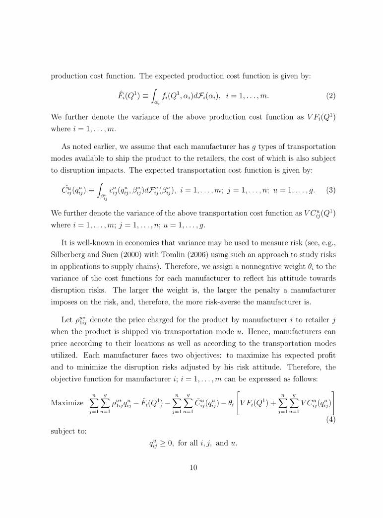
production cost function. The expected production cost function is given by:
Fi(Q1) ≡
∫αi
fi(Q1, αi)dFi(αi), i = 1, . . . ,m. (2)
We further denote the variance of the above production cost function as V Fi(Q1)
where i = 1, . . . ,m.
As noted earlier, we assume that each manufacturer has g types of transportation
modes available to ship the product to the retailers, the cost of which is also subject
to disruption impacts. The expected transportation cost function is given by:
Cuij(q
uij) ≡
∫βu
ij
cuij(q
uij, β
uij)dFu
ij(βuij), i = 1, . . . ,m; j = 1, . . . , n; u = 1, . . . , g. (3)
We further denote the variance of the above transportation cost function as V Cuij(Q
1)
where i = 1, . . . ,m; j = 1, . . . , n; u = 1, . . . , g.
It is well-known in economics that variance may be used to measure risk (see, e.g.,
Silberberg and Suen (2000) with Tomlin (2006) using such an approach to study risks
in applications to supply chains). Therefore, we assign a nonnegative weight θi to the
variance of the cost functions for each manufacturer to reflect his attitude towards
disruption risks. The larger the weight is, the larger the penalty a manufacturer
imposes on the risk, and, therefore, the more risk-averse the manufacturer is.
Let ρu∗1ij denote the price charged for the product by manufacturer i to retailer j
when the product is shipped via transportation mode u. Hence, manufacturers can
price according to their locations as well as according to the transportation modes
utilized. Each manufacturer faces two objectives: to maximize his expected profit
and to minimize the disruption risks adjusted by his risk attitude. Therefore, the
objective function for manufacturer i; i = 1, . . . ,m can be expressed as follows:
Maximizen∑
j=1
g∑u=1
ρu∗1ijq
uij − Fi(Q
1)−n∑
j=1
g∑u=1
Cuij(q
uij)− θi
V Fi(Q1) +
n∑j=1
g∑u=1
V Cuij(q
uij)
(4)
subject to:
quij ≥ 0, for all i, j, and u.
10

The first term in (4) represents the revenue. The second term is the expected
disruption related production cost. The third term is the expected disruption related
transportation cost. The fourth term is the cost of disruption risks adjusted by each
manufacturer’s attitude.
We assume that, for each manufacturer, the production cost function and the
transaction cost function without disruptions are continuously differentiable and con-
vex. It is easy to verify that Fi(Q1), V Fi(Q
1), Cuij(q
uij), and V Cu
ij(quij) are also continu-
ously differentiable and convex. Furthermore, we assume that manufacturers compete
in a noncooperative fashion in the sense of Nash (1950, 1951). Hence, the optimal-
ity conditions for all manufacturers simultaneously (cf. Bazaraa, Sherali, and Shetty
(1993) and Nagurney (1999)) can be expressed as the following variational inequality:
determine Q1∗ ∈ Rmng+ satisfying:
m∑i=1
n∑j=1
g∑u=1
∂Fi(Q1∗)
∂quij
+∂Cu
ij(qu∗ij )
∂quij
+ θi(∂V Fi(Q
1∗)
∂qu∗ij
+∂V Cu
ij(qu∗ij )
∂qu∗ij
)− ρu∗1ij
×[qu
ij − qu∗ij ] ≥ 0, ∀Q1 ∈ Rmng
+ . (5)
2.2 The Behavior of the Retailers
The retailers, in turn, are involved in transactions both with the manufacturers and
the demand markets since they must obtain the product to deliver to the consumers
at the demand markets.
Let ρv∗2jk denote the price charged for the product by retailer j to demand market
k when the product is shipped via transportation mode v. Hence, retailers can price
according to their locations as well as according to the transportation modes utilized.
This price is determined endogenously in the model along with the prices associated
with the manufacturers, that is, the ρu∗1ij, for all i, j and u. We assume that certain
disruptions will affect the retailers’ handling processes (e. g., the storage and display
processes). An additional random risk/disruption related random parameter ηj is
associated with the handling cost of retailer j. Recall that we also assume that there
are h types of transportation modes available to each retailer for shipping the product
11
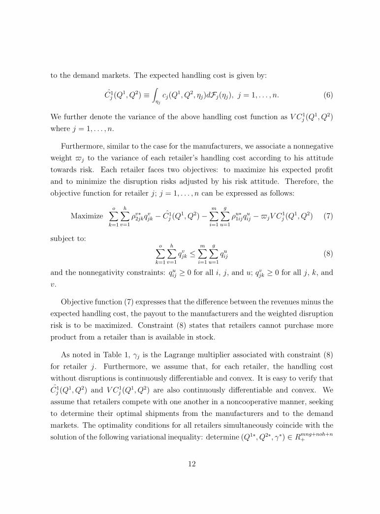
to the demand markets. The expected handling cost is given by:
C1j (Q1, Q2) ≡
∫ηj
cj(Q1, Q2, ηj)dFj(ηj), j = 1, . . . , n. (6)
We further denote the variance of the above handling cost function as V C1j (Q1, Q2)
where j = 1, . . . , n.
Furthermore, similar to the case for the manufacturers, we associate a nonnegative
weight $j to the variance of each retailer’s handling cost according to his attitude
towards risk. Each retailer faces two objectives: to maximize his expected profit
and to minimize the disruption risks adjusted by his risk attitude. Therefore, the
objective function for retailer j; j = 1, . . . , n can be expressed as follows:
Maximizeo∑
k=1
h∑v=1
ρv∗2jkq
vjk − C1
j (Q1, Q2)−m∑
i=1
g∑u=1
ρu∗1ijq
uij −$jV C1
j (Q1, Q2) (7)
subject to:o∑
k=1
h∑v=1
qvjk ≤
m∑i=1
g∑u=1
quij (8)
and the nonnegativity constraints: quij ≥ 0 for all i, j, and u; qv
jk ≥ 0 for all j, k, and
v.
Objective function (7) expresses that the difference between the revenues minus the
expected handling cost, the payout to the manufacturers and the weighted disruption
risk is to be maximized. Constraint (8) states that retailers cannot purchase more
product from a retailer than is available in stock.
As noted in Table 1, γj is the Lagrange multiplier associated with constraint (8)
for retailer j. Furthermore, we assume that, for each retailer, the handling cost
without disruptions is continuously differentiable and convex. It is easy to verify that
C1j (Q1, Q2) and V C1
j (Q1, Q2) are also continuously differentiable and convex. We
assume that retailers compete with one another in a noncooperative manner, seeking
to determine their optimal shipments from the manufacturers and to the demand
markets. The optimality conditions for all retailers simultaneously coincide with the
solution of the following variational inequality: determine (Q1∗, Q2∗, γ∗) ∈ Rmng+noh+n+
12
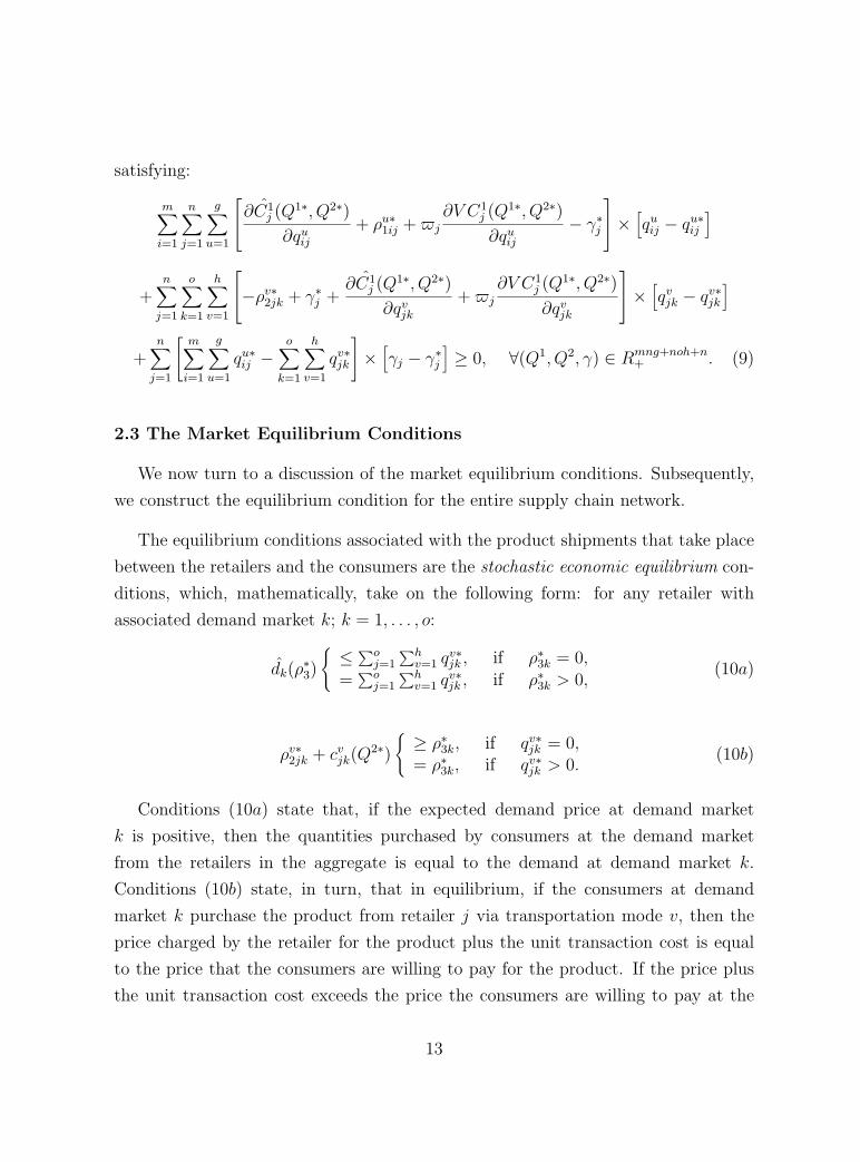
satisfying:
m∑i=1
n∑j=1
g∑u=1
∂C1j (Q1∗, Q2∗)
∂quij
+ ρu∗1ij + $j
∂V C1j (Q1∗, Q2∗)
∂quij
− γ∗j
× [quij − qu∗
ij
]
+n∑
j=1
o∑k=1
h∑v=1
−ρv∗2jk + γ∗
j +∂C1
j (Q1∗, Q2∗)
∂qvjk
+ $j
∂V C1j (Q1∗, Q2∗)
∂qvjk
× [qvjk − qv∗
jk
]
+n∑
j=1
[m∑
i=1
g∑u=1
qu∗ij −
o∑k=1
h∑v=1
qv∗jk
]×
[γj − γ∗
j
]≥ 0, ∀(Q1, Q2, γ) ∈ Rmng+noh+n
+ . (9)
2.3 The Market Equilibrium Conditions
We now turn to a discussion of the market equilibrium conditions. Subsequently,
we construct the equilibrium condition for the entire supply chain network.
The equilibrium conditions associated with the product shipments that take place
between the retailers and the consumers are the stochastic economic equilibrium con-
ditions, which, mathematically, take on the following form: for any retailer with
associated demand market k; k = 1, . . . , o:
dk(ρ∗3)
{≤ ∑o
j=1
∑hv=1 qv∗
jk , if ρ∗3k = 0,=
∑oj=1
∑hv=1 qv∗
jk , if ρ∗3k > 0,(10a)
ρv∗2jk + cv
jk(Q2∗)
{≥ ρ∗3k, if qv∗
jk = 0,= ρ∗3k, if qv∗
jk > 0.(10b)
Conditions (10a) state that, if the expected demand price at demand market
k is positive, then the quantities purchased by consumers at the demand market
from the retailers in the aggregate is equal to the demand at demand market k.
Conditions (10b) state, in turn, that in equilibrium, if the consumers at demand
market k purchase the product from retailer j via transportation mode v, then the
price charged by the retailer for the product plus the unit transaction cost is equal
to the price that the consumers are willing to pay for the product. If the price plus
the unit transaction cost exceeds the price the consumers are willing to pay at the
13

demand market then there will be no transaction between the retailer and demand
market via that transportation mode.
Equilibrium conditions (10a) and (10b) are equivalent to the following variational
inequality problem, after summing over all demand markets: determine (Q2∗, ρ∗3) ∈Rnoh+o
+ satisfying:o∑
k=1
(n∑
j=1
h∑v=1
qv∗jk − dk(ρ
∗3))× [ρ3k − ρ∗3k]
+o∑
k=1
n∑j=1
h∑v=1
(ρv∗2jk + cv
jk(Q2∗)− ρ∗3k)× [qv
jk − qv∗jk ] ≥ 0, ∀ρ3 ∈ Ro
+, ∀Q2 ∈ Rnoh+ , (11)
where ρ3 is the o-dimensional vector with components: ρ31, . . . , ρ3o and Q2 is the
noh-dimensional vector.
Remark: In this paper, we are interested in the cases where the expected demands
are positive, that is, dk(ρ3) > 0, ∀ρ3 ∈ Ro+ for k = 1, . . . , o. Furthermore, we assume
that the unit transaction costs: cvjk(Q
2) > 0, ∀j, k, ∀Q2 6= 0.
Under the above assumptions, we have that ρ∗3k > 0 and dk(ρ∗3) =
∑nj=1
∑ok=1
∑hv=1 qv∗
jk ,
∀k. This can be shown by contradiction. If there exists a k where ρ∗3k = 0, then ac-
cording to (10a) we have that∑n
j=1
∑ok=1
∑hv=1 qv∗
jk ≥ dk(ρ∗3) > 0. Hence, there exists
at least a (j,k) pair such that qv∗jk > 0, which means that cv
jk(Q2∗) > 0 by assumption.
From conditions (10b), we have that ρv∗2jk + cv
jk(Q2∗) = ρ3k > 0, which leads to a
contradiction.
2.4 The Equilibrium Conditions of the Supply Chain
In equilibrium, we must have that the optimality conditions for all manufacturers,
as expressed by (4), the optimality conditions for all retailers, as expressed by (9), and
as well as the equilibrium conditions for all the demand markets, as expressed by (11),
must hold simultaneously (see also Nagurney, Cruz, Dong, and Zhang (2005)). Hence,
the product shipments of the manufacturers with the retailers must be equal to the
product shipments that retailers accept from the manufacturers. We now formally
state the equilibrium conditions for the entire supply chain network as follows:
14

Definition 1: Supply Chain Network Equilibrium with Uncertainty and
Random Demands
The equilibrium state of the supply chain network with disruption risks and random
demands is one where the flows of the product between the tiers of the decision-makers
coincide and the flows and prices satisfy the sum of conditions (4), (9), and (11).
The summation of inequalities (4), (9), and (11), after algebraic simplification,
yields the following result (see also Nagurney (1999, 2006a)).
Theorem 1: Variational Inequality Formulation
A product shipment and price pattern (Q1∗, Q2∗, γ∗, ρ∗3) ∈ Rmng+noh+n+o+ is an equi-
librium pattern of the supply chain model according to Definition 1, if and only if it
satisfies the variational inequality problem:
m∑i=1
n∑j=1
g∑u=1
[∂Fi(Q
1∗)
∂quij
+∂Cu
ij(qu∗ij )
∂quij
+ θi(∂V Fi(Q
1∗)
∂quij
+∂V Cu
ij(qu∗ij )
∂quij
)
+∂C1
j (Q1∗, Q2∗)
∂quij
+ $j
∂V C1j (Q1∗, Q2∗)
∂quij
− γ∗j ]× [qu
ij − qu∗ij ]
+n∑
j=1
o∑k=1
g∑v=1
[∂C1
j (Q1∗, Q2∗)
∂qvjk
+ $j
∂V C1j (Q1∗, Q2∗)
∂qvjk
+γ∗j + cv
jk(Q2∗)− ρ∗3k]×
[qvjk − qv∗
jk
]+
n∑j=1
[m∑
i=1
g∑u=1
qu∗ij −
o∑k=1
h∑v=1
qv∗jk
]×
[γj − γ∗
j
]+
o∑k=1
(n∑
j=1
h∑v=1
qv∗jk − dk(ρ
∗3))× [ρ3k − ρ∗3k] ≥ 0,
∀(Q1, Q2, γ, ρ3) ∈ Rmng+noh+n+o+ . (12)
For easy reference in the subsequent sections, variational inequality problem (12)
can be rewritten in standard variational inequality form (cf. Nagurney (1999)) as
follows: determine X∗ ∈ K:
〈F (X∗), X −X∗〉 ≥ 0, ∀X ∈ K ≡ Rmng+noh+n+o+ , (13)
15
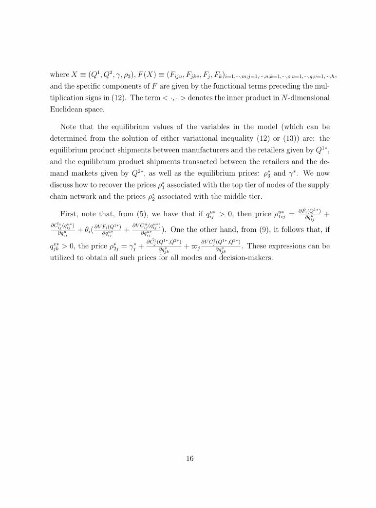
where X ≡ (Q1, Q2, γ, ρ3), F (X) ≡ (Fiju, Fjkv, Fj, Fk)i=1,···,m;j=1,···,n;k=1,···,o;u=1,···,g;v=1,···,h,
and the specific components of F are given by the functional terms preceding the mul-
tiplication signs in (12). The term < ·, · > denotes the inner product in N -dimensional
Euclidean space.
Note that the equilibrium values of the variables in the model (which can be
determined from the solution of either variational inequality (12) or (13)) are: the
equilibrium product shipments between manufacturers and the retailers given by Q1∗,
and the equilibrium product shipments transacted between the retailers and the de-
mand markets given by Q2∗, as well as the equilibrium prices: ρ∗3 and γ∗. We now
discuss how to recover the prices ρ∗1 associated with the top tier of nodes of the supply
chain network and the prices ρ∗2 associated with the middle tier.
First, note that, from (5), we have that if qu∗ij > 0, then price ρu∗
1ij = ∂Fi(Q1∗)
∂quij
+
∂Cuij(q
u∗ij )
∂quij
+ θi(∂V Fi(Q
1∗)∂qu∗
ij+
∂V Cuij(q
u∗ij )
∂qu∗ij
). One the other hand, from (9), it follows that, if
qv∗jk > 0, the price ρ∗2j = γ∗
j +∂C1
j (Q1∗,Q2∗)
∂qvjk
+ $j∂V C1
j (Q1∗,Q2∗)
∂qvjk
. These expressions can be
utilized to obtain all such prices for all modes and decision-makers.
16
3. A Weighted Supply Chain Performance Measure
In this Section, we first propose a supply chain network performance measure.
Then, we provide the definition of supply chain network robustness, and follow with
the definition for a weighted supply chain performance measure.
3.1 A Supply Chain Network Performance Measure
Recently, Qiang and Nagurney (2008) (see also Nagurney and Qiang (2007a, b, c))
proposed a network performance measure, which captures flows, costs, and behavior
under network equilibrium conditions. Based on the measure in the above paper(s),
we propose the following definition of a supply chain network performance measure.
Definition 2: The Supply Chain Network Performance Measure
The supply chain network performance measure, E, for a given supply chain, and
expected demands: dk; k = 1, 2, . . . , o, is defined as follows:
E ≡∑o
k=1dk
ρ3k
o, (14)
where o is the number of demand markets in the supply chain network, and dk and
ρ3k denote, respectively, the expected equilibrium demand and the equilibrium price at
demand market k.
Note that the equilibrium price is equal to the unit production and transaction
costs plus the weighted marginal risks for producing and transacting one unit from
the manufacturers to the demand markets (see also Nagurney (2006b)). According
to the above performance measure, a supply chain network performs well in network
equilibrium if, on the average, and across all demand markets, a large demand can
be satisfied at a low price. Therefore, in this paper, we apply the above performance
measure to assess the robustness of particular supply chain networks. From the
discussion in Section 2.3, we have that ρ3k > 0, ∀k. Therefore, the above definition
is well-defined.
Furthermore, since each individual may have different opinions as to the risks, we
need a “basis” to compare supply chain performance under different risk attitudes and
17
to understand how risk attitudes affect the performance of a supply chain. Hence,
we define E0 as the supply chain performance measure where the dk and the ρ3k;
k = 1, . . . , o, are obtained by assuming that the weights that reflect the manufacturers
and the retailers’ attitudes towards the disruption risks are zero. This definition
excludes individuals’ subjective differences in a supply chain and, with this definition,
we are ready to study supply chain network robustness.
3.2 Supply Chain Robustness Measurement
Robustness has a broad meaning and is often couched in different settings. Gener-
ally speaking, robustness means that the system performs well when exposed to un-
certain future conditions and perturbations (cf. Bundschuh, Klabjan, and Thurston
(2003), Snyder (2003), and Holmgren (2007)).
Therefore, we propose the following rationale to assess the robustness of a supply
chain: assume that all the random parameters take on a given threshold probability
value; say, for example, 95%. Moreover, assume that all the cumulative distribution
functions for random parameters have inverse functions. Hence, we have that: αi =
F−1i (.95), for i = 1, . . . ,m; βu
ij = Fu−1
ij (.95), for i = 1, . . . ,m; j = 1, . . . , n, and so
on. With the disruption related parameters given, we can calculate the supply chain
performance measure according to the definition given by (14). Let Ew denote the
supply chain performance measure with random parameters fixed at a certain level
as described above. For example, when w = 0.95, Ew is the supply chain performance
with all the random risk parameters fixed at the value of a 95% probability level.
Then, the supply chain network robustness measure, R, is given by the following:
R = E0 − Ew, (15)
where E0 gauges the supply chain performance based on the model introduced in
Section 2, but with weights related to risks being zero.
E0 examines the “base” supply chain performance while Ew assesses the supply
chain performance measure at some prespecified uncertainty level. If their difference
is small, a supply chain maintains its functionality well and we consider the supply
18
chain to be robust at the threshold disruption level. Hence, the lower the value of R,
the more robust a supply chain is.
Notably, the above robustness definition has implications for network resilience as
well. Resilience is a general and conceptual term, which is hard to quantify. McCarthy
(2007) defined resilience “... as the ability of a system to recover from adversity, ei-
ther back to its original state or an adjusted state based on new requirements, ...”.
For a comprehensive discussion of resilience, please refer to the Critical Infrastruc-
ture Protection Program (2007). Because our supply chain measure is based on the
network equilibrium model, a network that is qualified as being robust according to
our measure is also resilient provided that its performance after experiencing the dis-
ruption(s) is close to the “original value.” Interestingly, this idea is in agreement with
Hansson and Helgesson (2003), who proposed that robustness can be treated as a
special case of resilience.
3.3 A Weighted Supply Chain Performance Measure
Note that different supply chains may have different requirements regarding the
performance and robustness concepts introduced in the previous sections. For ex-
ample, in the case of a supply chain of a toy product one may focus on how to
satisfy demand in the most cost efficient way and not care too much about sup-
ply chain robustness. A medical/healthcare supply chain, on the other hand, may
have a requirement that the supply chain be highly robust when faced with uncer-
tain conditions. Hence, in order to be able to examine and to evaluate the different
application-based supply chains from both perspectives, we now define a weighted
supply chain performance measure as follows:
E = (1− ε)E0 + ε(−R), (16)
where ε ∈ [0, 1] is the weight that is placed on the supply chain robustness.
When ε is equal to 1, the performance of a supply chain hinges only on the robust-
ness measure, which may be the case for a medical/healthcare supply chain, noted
above. In contrast, when ε is equal to 0, the performance of the supply chain depends
19

solely on how well it can satisfy demands at low prices. The supply chain of a toy
product in the above discussion falls into this category.
4. Examples
The supply chain network topology for the numerical examples is depicted in
Figure 2 below. There are assumed to be two manufacturers, two retailers, and two
demand markets. There are two modes of transportation available between each
manufacturer and retailer pair and between each retailer and demand market pair.
These examples are solved by the modified projection method of Korpelevich (1977);
see also, e.g., Nagurney (2006a).
Demand Markets
� ��1 � ��
2
Manufacturers
Retailers
� ��1 � ��
2
� ��1 � ��
2?
��
��
�
@@
@@
@R?
?
��
��
�
@@
@@
@R?
Figure 2: The Supply Chain Network for the Numerical Examples
Example 1
In the first example, for illustration purposes, we assumed that all the random pa-
rameters followed uniform distributions. The relevant parameters are as follows:
20

αi ∼ [0, 2] for i = 1, 2; βuij ∼ [0, 1] for i = 1, 2; j = 1, 2; u = 1, 2; ηj ∼ [0, 3] for
j = 1, 2.
We further assumed that the demand functions followed a uniform distribution
given by [200− 2ρ3k, 600− 2ρ3k], for k = 1, 2. Hence, the expected demand functions
are:
dk(ρ3) = 400− 2ρ3k, for k = 1, 2.
The production cost functions for the manufacturers are given by:
f1(Q1, α1) = 2.5(
2∑j=1
2∑u=1
qu1j)
2 + (2∑
j=1
2∑u=1
qu1j)(
2∑j=1
2∑u=1
qu2j) + 2α1(
2∑j=1
2∑u=1
qu1j),
f2(Q1, α2) = 2.5(
2∑j=1
2∑u=1
qu2j)
2 + (2∑
j=1
2∑u=1
qu1j)(
2∑j=1
2∑u=1
qu2j) + 2α2(
2∑j=1
2∑u=1
qu2j).
The expected production cost functions for the manufacturers are given by:
F1(Q1) = 2.5(
2∑j=1
2∑u=1
qu1j)
2 + (2∑
j=1
2∑u=1
qu1j)(
2∑j=1
2∑u=1
qu2j) + 2(
2∑j=1
2∑u=1
qu1j),
F2(Q1) = 2.5(
2∑j=1
2∑u=1
qu2j)
2 + (2∑
j=1
2∑u=1
qu1j)(
2∑j=1
2∑u=1
qu2j) + 2(
2∑j=1
2∑u=1
qu2j).
The variances of the production cost functions for the manufacturers are given by:
V F1(Q1) =
4
3(
2∑j=1
2∑u=1
qu1j)
2,
V F2(Q1) =
4
3(
2∑j=1
2∑u=1
qu2j)
2.
The transaction cost functions faced by the manufacturers and associated with
transacting with the retailers are given by:
c1ij(q
1ij, β
1ij) = .5(q1
ij)2 + 3.5β1
ijq1ij, for i = 1, 2; j = 1, 2,
c2ij(q
2ij, β
2ij) = (q2
ij)2 + 5.5β2
ijq2ij, for i = 1, 2; j = 1, 2.
21

The expected transaction cost functions faced by the manufacturers and associated
with transacting with the retailers are given by:
C1ij(q
1ij) = .5(q1
ij)2 + 1.75q1
ij, for i = 1, 2; j = 1, 2,
C2ij(q
2ij) = .5(q2
ij)2 + 2.75q2
ij, for i = 1, 2; j = 1, 2.
The variances of the transaction cost functions faced by the manufacturers and
associated with transacting with the retailers are given by:
V C1ij(q
1ij) = 1.0208(q1
ij)2, for i = 1, 2; j = 1, 2,
V C2ij(q
2ij) = 2.5208(q2
ij)2, for i = 1, 2; j = 1, 2.
The handling costs of the retailers, in turn, are given by:
cj(Q1, Q2, ηj) = .5(
2∑i=1
2∑u=1
quij)
2 + ηj(2∑
i=1
2∑u=1
quij), for j = 1, 2.
The expected handling costs of the retailers are given by:
C1j (Q1, Q2) = .5(
2∑i=1
2∑u=1
quij)
2 + 1.5(2∑
i=1
2∑u=1
quij), for j = 1, 2.
The variance of the handling costs of the retailers are given by:
V Cj(Q1, Q2) =
3
4(
2∑i=1
2∑u=1
quij)
2, for j = 1, 2.
The unit transaction costs from the retailers to the demand markets are given by:
c1jk(Q
2) = .3q1jk, for j = 1, 2; k = 1, 2,
c2jk(Q
2) = .6q2jk, for j = 1, 2; k = 1, 2.
We assumed that the manufacturers and the retailers placed zero weights on the
disruption risks as discussed in Section 3.1 to compute E0.
22
In the equilibrium, under the expected costs and demands, we have that the
equilibrium shipments between manufacturers and retailers are: q1∗ij = 8.5022, for i =
1, 2; j = 1, 2; q2∗ij = 3.7511, for i = 1, 2; j = 1, 2; whereas the equilibrium shipments
between the retailers and the demand markets are: q1∗jk = 8.1767, for j = 1, 2; k =
1, 2; q2∗jk = 4.0767, for j = 1, 2; k = 1, 2. Finally, the equilibrium prices are: ρ∗31 =
ρ∗32 = 187.7466 and the expected equilibrium demands are: d1 = d2 = 24.5068.
The supply chain performance measure is equal to E0 = 0.1305. Now, assume that
w = .95; that is, all the random cost parameters are fixed at a 95% probability level.
The resulting supply chain performance measure is computed as Ew=0.1270. If we
let ε = .5 (cf. (16)), which means that we place equal emphasis on performance and
robustness of the supply chain, the weighted supply chain performance measure is
E = 0.0635.
Example 2
For the same network structure and cost and demand functions, we now assume that
the relevant parameters are changed as follows: αi ∼ [0, 4] for i = 1, 2; βuij ∼ [0, 2] for
i = 1, 2; j = 1, 2; u = 1, 2; ηj ∼ [0, 6] for j = 1, 2.
In the equilibrium, under the expected costs and demands, we have that the equi-
librium shipments between manufacturers and retailers are now: q1∗ij = 8.6008, for i =
1, 2; j = 1, 2; q2∗ij = 3.3004, for i = 1, 2; j = 1, 2; whereas the equilibrium ship-
ments between the retailers and the demand markets are: q1∗jk = 7.9385, for j =
1, 2; k = 1, 2; q2∗jk = 3.9652, for j = 1, 2; k = 1, 2. Finally, the equilibrium prices are:
ρ∗31 = ρ∗32 = 188.0963 and the expected equilibrium demands are: d1 = d2 = 23.8074.
The supply chain performance measure is equal to E0 = 0.1266. Similar to the above
example, let us assume that w = .95; that is, all the random cost parameters are
fixed at a 95% probability level. The resulting supply chain performance measure is
now: Ew=0.1194. If we let ε = .5, the weighted supply chain performance measure is
E = 0.0597.
Observe that first example leads to a better measure of performance since the
uncertain parameters do not have as great of an impact as in the second one for the
23

cost functions under the given threshold level.
5. Summary and Conclusions
In this paper, we developed a novel supply chain network model to study the
demand-side as well as the supply-side risks, with the demand being random and the
supply-side risks modeled as uncertain parameters in the underlying cost functions.
This supply chain model generalizes several existing models by including multiple
transportation modes from the manufacturers to the retailers, and from the retailers
to the demand markets. We also proposed a weighted supply chain performance and
robustness measure based on our recently derived network performance/efficiency
measure and illustrated the supply chain network model through numerical exam-
ples for which the equilibrium prices and product shipments were computed and
robustness analyses conducted. For future research, we plan on constructing further
comprehensive metrics in order to evaluate supply chain network performance and
to also apply the results in this paper to empirically-based supply chain networks in
different industries.
Acknowledgment The research of the first two authors was supported by the John
F. Smith Memorial Fund at the Isenberg School of Management. This support is
gratefully appreciated.
The authors would like to thank Professor Teresa Wu of Arizona State Univer-
sity and Professor Jennifer Blackhurst of Iowa State University for the invitation to
contribute this chapter to the volume Managing Supply Chain Risk and Vul-
nerability: Tools and Methods for Supply Chain Decision Makers, Springer.
24
References
M. S. Bazaraa, H. D. Sherali, and C. M. Shetty (1993). Nonlinear Programming:
Theory and Algorithms, John Wiley & Sons, New York.
B. M. Beamon (1998). “Supply chain design and analysis: models and methods,”
International Journal of Production Economics 55, 281-294.
B. M. Beamon (1999). “Measuring supply chain performance,” International Journal
of Operations and Production Management 19, 275-292.
M. Bundschuh, D. Klabjan, and D. L. Thurston (2003). “Modeling robust and reliable
supply chains,” Optimization Online e-print. www.optimization-online.org.
Canadian Competition Bureau (2006). “Competition bureau concludes examination
into gasoline price spike following hurricane Katrina,” http://www.competitionbureau.gc.ca
C. W. Craighead, J. Blackhurst, M. J. Rungtusanatham, and R. B. Handfield (2007).
“The severity of supply chain disruptions: Design characteristics and mitigation ca-
pabilities,” Decision Sciences 38, 131-156.
J. Dong, D. Zhang, and A. Nagurney (2002). “Supply chain networks with multi-
criteria decision-makers.” In Transportation and Traffic Theory in the 21st
Century, M. A. P., Editor, Pergamon, pp. 179-196.
J. Dong, D. Zhang, H. Yan, and A. Nagurney (2005). “Multitiered supply chain
networks: Multicriteria decision-making under uncertainty,” Annals of Operations
Research 135, 155-178.
Fairtrade Foundation (2002). “Spilling the bean,” http://www.fairtrade.org.uk.
D. Gupta (1996). “The (Q, r) inventory system with an unreliable supplier,” INFOR
34, 59-76.
S. O. Hansson and G. Helgesson (2003). “What is stability?” Synthese 136, 219-235.
25
K. B. Hendricks and V. R. Singhal (2005). “An empirical analysis of the effect of
supply chain disruptions on long-term stock price performance and risk of the firm,”
Production and Operations Management 14, 35-52.
A. J. Holmgren (2007). “A framework for vulnerability assessment of electric power
systems.” In Reliability and Vulnerability in Critical Infrastructure: A Quan-
titative Geographic Perspective, A. Murray and T. Grubesic, Editors, Springer-
Verlag, New York.
P. R. Kleindorfer and G. H. Saad (2005). “Managing disruption risks in supply
chains,” Production and Operations Management 14, 53-68.
G. M. Korpelevich (1977). “The extragradient method for finding saddle points and
other problems,” Matekon 13, 35-49.
K. H. Lai, E. W. T. Ngai, and T. C. E. Cheng (2002). “Measures for evaluating supply
chain performance in transport logistics,” Transportation Research E 38, 439-456.
D. M. Lambert and T. L. Pohlen (2001). “Supply chain metrics,” International
Journal of Logistics Management 12, 1-19.
A. Latour (2001). “Trial by fire: a blaze in Albuquerque sets off major crisis for
cell-phone giants,” Wall Street Journal, January 29.
H. Lee and S. Whang (1999). “Decentralized multi-echelon supply chains: Incentives
and information,” Management Science 45, 633-640.
J. A. McCarthy (2007). “From protection to resilience: injecting ‘Moxie’ into the
infrastructure security continuum,” Critical Infrastructure Protection Program, Dis-
cussion Paper Series, George Mason University, Fairfax, Virginia.
A. Nagurney (1999). Network Economics: A Variational Inequality Ap-
proach, second and revised edition, Kluwer Academic Publishers, Dordrecht, The
Netherlands.
26

A. Nagurney (2006a). Supply Chain Network Economics: Dynamics of Prices,
Flows, and Profits, Edward Elgar Publishing, Cheltenham, England.
A. Nagurney (2006b). “On the relationship between supply chin and transportation
network equilibria: A supernetwork equivalence with computations,” Transportation
Research E 42, 293-316.
A. Nagurney, J. Cruz, J. Dong, and D. Zhang (2005). “Supply chain networks,
electronic commerce, and supply side and demand side risk,” European Journal of
Operational Research 164, 120-142.
A. Nagurney, J. Dong, and D. Zhang (2002). “A supply chain network equilibrium
model,” Transportation Research E 38, 281-303.
A. Nagurney and Q. Qiang (2007a). “A transportation network efficiency measure
that captures flows, behavior, and costs with applications to network component
importance identification and vulnerability,” Proceedings of the POMS Conference,
Dallas, Texas, May 4-7.
A. Nagurney and Q. Qiang (2007b). “A network efficiency measure with application
to critical infrastructure networks,” Journal of Global Optimization 40, 261-275.
A. Nagurney and Q. Qiang (2007c). “A network efficiency measure for congested
networks,” Europhysics Letters 79, 38005.
J. F. Nash (1950). “Equilibrium points in n-person games,” Proceedings of the Na-
tional Academy of Sciences USA 36, 48-49.
J. F. Nash (1951). “Noncooperative games,” Annals of Mathematics 54, 286-298.
M. Parlar (1997). “Continuous review inventory problem with random supply inter-
ruptions,” European Journal of Operations Research 99, 366-385.
M. Parlar and D. Perry (1996). “Inventory models of future supply uncertainty with
single and multiple suppliers,” Naval Research Logistics 43, 191-210.
27

Q. Qiang and A. Nagurney (2008). “A unified network performance measure with im-
portance identification and the ranking of network components,” Optimization Letters
2, 127-142.
T. Santoso, S. Ahmed, M. Goetschalckx, and A. Shapiro (2005). “A stochastic pro-
gramming approach for supply chain network design under uncertainty,” European
Journal of Operations Research 167, 96-115.
Y. Sheffi (2005). The Resilient Enterprise: Overcoming Vulnerability for
Competitive Advantage, MIT Press, Cambridge, Massachusetts.
E. Silberberg and W. Suen (2000). The Structure of Economics: A Mathemat-
ics Analysis, Mcgraw-Hill, New York.
L. V. Snyder (2003). “Supply chain robustness and reliability: models and algo-
rithms,” Ph.D. dissertation, Northwestern University, Department of Industrial En-
gineering and Management Sciences, Evanston, Illinois.
L. V. Snyder and Z.-J. M. Shen (2006). “Supply chain management under the threat
of disruptions,” The Bridge 36, 39-45.
L. V. Snyder and M. S. Daskin (2005). “A reliability model for facility location: the
expected failure cost case,” Transportation Science 39, 400-416.
C. S. Tang (2006a). “Robust strategies for mitigating supply chain disruptions,”
International Journal of Logistics 9, 33-45.
C. S. Tang (2006b). “Perspectives in supply chain risk management,” International
Journal of Production Economics 103, 451-488.
B. T. Tomlin (2006). “On the value of mitigation and contingency strategies for
managing supply chain disruption risks,” Management Science 52, 639-657.
S. M. Wagner and C. Bode (2007). “An empirical investigation into supply chain
vulnerability,” Journal of Purchasing and Supply Management 12, 301-312.
28
M. C. Wilson (2007). “The impact of transportation disruptions on supply chain
performance,” Transportation Research E 43, 295-320.
T. Wu, J. Blackhurst, and V. Chidambaram (2006). “The model for inbound supply
risk analysis,” Computers in Industry 57, 350-365.
29


