
Department of Comparative Linguistics
Balthasar Bickel
Modeling the Diachrony of Grammar: which data? which methods?

Why statistical modeling?
• modeling type transition trends for testing evolutionary hypothesis, e.g.,
• on biological constraints on how languages evolve
• on repeated contact effects skewing diachronies in large areas
2
• classical comparative linguistics has not been very successful in reconstructing abstract grammatical patterns
• ancient data is extremely rare and has severe sampling problems
O
N3-TAT
N2-P43
N
N1-M128
N*-M231(xN1,N2,N3)
a
b c
d e
f g
NO*-M214(xM231,M175)
Figure 2 Geographical distribution of NO clade. (a–g) Spatial frequency distributions of the NO clade: NO*, N (overall distribution of hg N), O(overall distribution of hg O), N*, N1, N2, N3. Maps are based on data from Supplementary Table 1. We label various panels following the YCC ‘bymutation’ format by adding the relevant mutation suffix.
Origin and phylogeography of Y-haplogroup NS Rootsi et al
206
European Journal of Human Genetics
0.5 1.0
−4
4
sµV
F3 FZ F4
FC1 FC2
CZ
CP1 CP2
P3 PZ P4
N400
PERFECTIVE ASPECT
PERF−AMB (n=32)PERF−CON (n=32)
LPS
APUP
Bickel et al. 2015 PLOS ONE
Bickel 2015 CUP HB Areal Linguistics

*Stud. Lang, +PNAS, †PNAS, ‡Phon. Domains, §Ling Typ, #Lang Dyn Change, ¶Ling Typ, ‖Ling Typ
Available methods: the tradition
• Search for diachronic trends by counting structures
• Family relations are an obvious confound (Galton’s Problem, Simpson’s Paradox), so control for them by…:
• strategic sampling (Dryer 1989*), or re-sampling (Everett et al. 2015+)
• modeling them as fixed (Dediu & Ladd 2007†, Bickel et al. 2009‡) or random (Jaeger et al. 2011§, Bentz & Winter 2013#) factors
• but even after controling for confounds, synchronic frequencies ⇏ transition probabilities:
• the process may not have reached stationarity (Maslova 2000¶)
• indeed sometimes has not reached stationarity (Cysouw 2011‖),
3
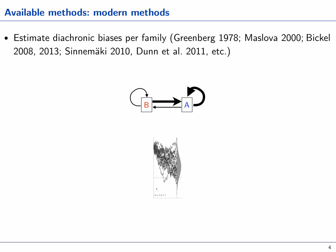
Available methods: modern methods
• Estimate diachronic biases per family (Greenberg 1978; Maslova 2000; Bickel 2008, 2013; Sinnemäki 2010, Dunn et al. 2011, etc.)
4
Model-Based Comparative Analysis 685
Figure 1: Effect of varying j in a Brownian motion (BM) process. Plottedare random walks through time for a continuous character with phe-notypic value along the Y-axis and time along the X-axis. At each smallstep in time, the phenotype has an equal and independent probabilityof increasing or decreasing in value. Increasing j results in strongerrandom drift and a broader distribution of final states. Because Ornstein-Uhlenbeck (OU) processes contain a drift component, increasing j alsobroadens the distribution of final states in OU processes. Each paneldisplays 30 realizations of the stochastic process and the distribution offinal states (the Gaussian curves to the right of the random walks). Theprocess is simulated from to , with each realization havingt p 0 t p 1the same initial state. An animation of this process is provided in theonline edition of the American Naturalist.
Figure 2: Influence of the selection-strength parameter a and optimumtrait value v on a trait evolving under an Ornstein-Uhlenbeck (OU)process. Larger values of a imply stronger selection and hence a morerapid approach to the optimum value v (dotted line) as well as a tighterdistribution of phenotypes around the optimum. Each panel displays 20realizations of the OU process and the distribution of final trait values.The process is simulated from to , with each realization havingt p 0 t p 1the same initial state and value of v. See figure 1 for explanation of axes.
This term is linear in X, so it is as simple as it mightpossibly be. It contains two additional parameters: a mea-sures the strength of selection, and v gives the optimumtrait value. The force of selection is proportional to thedistance, , of the current trait value from the op-v ! X(t)timum. Thus, if the phenotype has drifted far from theoptimum, the “pull” toward the optimum will be verystrong, whereas if the phenotype is currently at the opti-mum, selection will have no effect until the stochasticitymoves the phenotype away from the optimum again orthere is a change in the optimum, v, itself. Because of itsdependence on the distance from the optimum, the OUprocess can be used to model stabilizing selection. Theeffect of varying a can be seen in figure 2.
Because the OU model reduces to BM when , ita p 0can be viewed as an elaboration of the BM model. As astatistical model, its primary justification is to be soughtin the fact that it represents a step beyond BM in thedirection of realism while yet remaining mathematicallytractable. As a model of evolution, the OU process is con-
sistent with a variety of evolutionary interpretations, twoof which we mention here.
Lande (1976) showed that under certain assumptions,evolution of the species’ mean phenotype can take theform of an OU process. In Lande’s formulation, both nat-ural selection and random genetic drift are assumed to acton the phenotypic character; the OU process’s optimum
denotes the location of a local maximum in a fitnessvlandscape. Felsenstein (1988) pointed out that in the eventthat this optimum itself moves randomly, the correct de-scription of the phenotypic evolution is no longer exactlyan OU process, but an OU process remains a goodapproximation.
Hansen (1997) raised questions concerning the time-scale of the approach of a species’ mean phenotype to itsoptimal value relative to that of macroevolution. Specifi-cally, he suggested that the macroevolutionary OU processhe proposed could only operate on far too slow a timescaleto be identical with the Landean OU process (cf. Lande1980). He proposed a different interpretation based on thesupposition that at any point in its history, a given phe-notypic character is subject to a large number of conflictingselective demands (genetic and environmental) so that itspresent value is the outcome of a compromise among
B A
*B
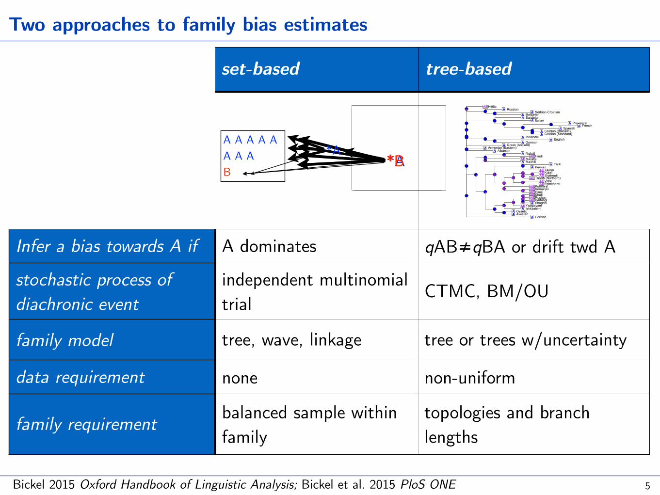
set-based tree-based
Infer a bias towards A if A dominates qAB≠qBA or drift twd A
stochastic process of diachronic event
independent multinomial trial CTMC, BM/OU
family model tree, wave, linkage tree or trees w/uncertainty
data requirement none non-uniform
family requirement balanced sample within family
topologies and branch lengths
Bickel 2015 Oxford Handbook of Linguistic Analysis; Bickel et al. 2015 PloS ONE
Two approaches to family bias estimates
5
glottolog.org (Hammarström & Nordhoff 2014)
The Family Bias Method: Indo-European
Set-based: P(E≻A) > P(A≻E), p<.001
32
Albanian
AvestanOssetic
IshkashimiYazgulyam
BartangiShughni
KhufiRushan
DimiliKirmanjki
EshtehardiVafsi
Talysh (Northern)ShahrudiKajaliTarom
Kurmanjî
PersianTajik
HindiNahali
MaithiliMarathi
BulgarianSerbian-Croatian
Russian
Catalan (Balearic)Catalan (Standard)
SpanishFrench (colloquial)
ProvencalItalian
Sardinian
Cornish
GermanEnglish
Icelandic
Greek (Ancient)
Hittite
Armenian (Eastern)A
AA
AAE
AEA
AEAEAEAE
AEAE
AEAEAEAE
AE
AA
AEA
AAE
AA
A
AA
AA
AA
A
A
AA
A
A
AE
A
Tree-based, P(E≻A) ≈ P(A≻E) ML logBF=.08 (p=.77)
(Topology and branch lengths based on nodes in Glottolog)
A A A A A A A A B
*A*B *A
*B

Witzlack-Makarevich, Zakharko, Bierkandt, Zúñiga & Bickel 2016 Linguistics
Continuous variables: trends in paradigms
• Case study on referential scales shaping agreement paradigms
6
2 ≻ 1 2 ≻ 3
→
→
• How many slots show such competition, and when they do, who wins? • Any diachronic trends, drifts?

Witzlack-Makarevich, Zakharko, Bierkandt, Zúñiga & Bickel 2016 Linguistics
Continuous variables: trends in paradigms
A. Set-based family bias test: • data-point = binomial test of rankings per paradigm
• family bias if a given ranking is significant for the majority of paradigms • Results:
• Algonquain slightly biased towards 1≻3 and 2≻3 (63%) • Kiranti is not biased towards any ranking ever
7
19
Language TAM 1≻2 2≻1 1≻3 3≻1 2≻3 3≻2Athpare IND 0 4 2 1 4 0
BahingNPST.IND 4 0 8 0 2 0PST.IND 4 0 8 0 2 0
Bantawa IND 0 0 1 0 1 0
Belhare IND 8 2 0 0 1 0
Camling IND 2 1 8 0 13 0
Chintang NPST.IND 9 6 14 0 3 0
Dumi NPST.IND 5 0 0 0 2 0
Jero IND 3 0 1 0 4 0
KõicNPST.IND 4 4 5 4 4 3PST.IND 7 4 5 4 3 4
KoyiNPST.IND 8 0 17 0 4 0PST.IND 8 0 14 3 4 0
KulungNPST.IND 3 1 4 0 4 0PST.IND 3 3 4 0 4 0
LimbuNPST.IND 0 0 0 0 6 6PST.IND 0 0 0 0 6 6
LohorungNPST.IND 0 0 4 6 0 1PST.IND 0 0 4 6 0 1
PumaNPST.IND 2 6 7 2 12 1PST.IND 2 6 7 2 12 1
Wambule IND 1 3 5 0 3 0
Yamphu IND 3 3 1 3 2 1
Table 6: Pairwise ranking of person values in the Kiranti languages
Language 1>2 2>1 1>3 3>1 2>3 3>2
Arapaho 0 6 21 9 20 0
Blackfoot 2 8 4 0 0 0
Cheyenne 2 12 28 2 16 2
Eastern Ojibwa 2 8 28 0 16 0
Micmac 10 2 56 30 48 6
Munsee 2 8 28 6 16 6
Passamaquoddy 0 8 24 12 16 12
Plains Cree 4 10 48 12 27 10
Table 7: Pairwise ranking of person values in the Algonquian languages
DRAFT – February 17, 2015
1≻3 because 21 out of 30 is significant under a binomial test
Witzlack-Makarevich, Zakharko, Bierkandt, Zúñiga & Bickel 2016 Linguistics
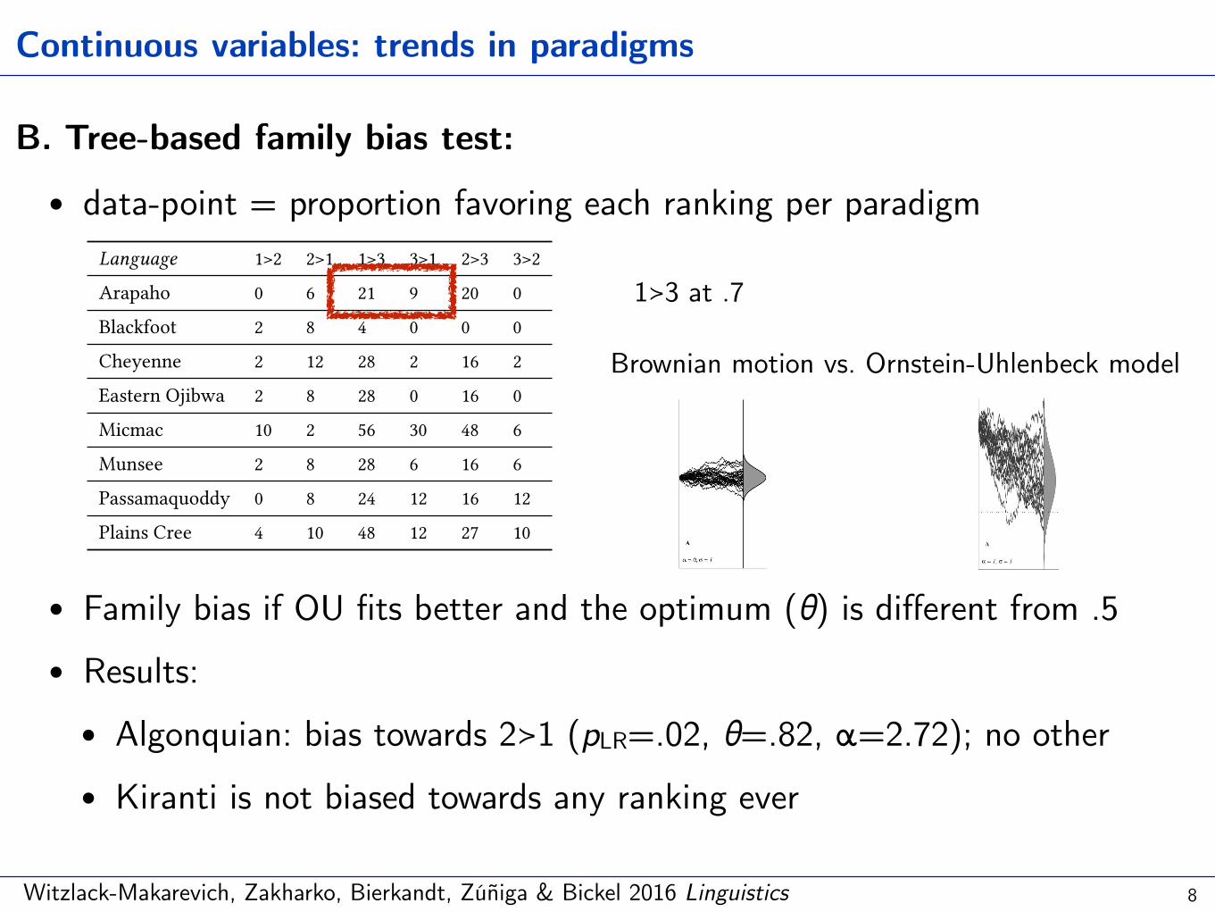
Continuous variables: trends in paradigms
B. Tree-based family bias test: • data-point = proportion favoring each ranking per paradigm
• Family bias if OU fits better and the optimum (θ) is different from .5 • Results:
• Algonquian: bias towards 2≻1 (pLR=.02, θ=.82, α=2.72); no other • Kiranti is not biased towards any ranking ever
8
19
Language TAM 1≻2 2≻1 1≻3 3≻1 2≻3 3≻2Athpare IND 0 4 2 1 4 0
BahingNPST.IND 4 0 8 0 2 0PST.IND 4 0 8 0 2 0
Bantawa IND 0 0 1 0 1 0
Belhare IND 8 2 0 0 1 0
Camling IND 2 1 8 0 13 0
Chintang NPST.IND 9 6 14 0 3 0
Dumi NPST.IND 5 0 0 0 2 0
Jero IND 3 0 1 0 4 0
KõicNPST.IND 4 4 5 4 4 3PST.IND 7 4 5 4 3 4
KoyiNPST.IND 8 0 17 0 4 0PST.IND 8 0 14 3 4 0
KulungNPST.IND 3 1 4 0 4 0PST.IND 3 3 4 0 4 0
LimbuNPST.IND 0 0 0 0 6 6PST.IND 0 0 0 0 6 6
LohorungNPST.IND 0 0 4 6 0 1PST.IND 0 0 4 6 0 1
PumaNPST.IND 2 6 7 2 12 1PST.IND 2 6 7 2 12 1
Wambule IND 1 3 5 0 3 0
Yamphu IND 3 3 1 3 2 1
Table 6: Pairwise ranking of person values in the Kiranti languages
Language 1>2 2>1 1>3 3>1 2>3 3>2
Arapaho 0 6 21 9 20 0
Blackfoot 2 8 4 0 0 0
Cheyenne 2 12 28 2 16 2
Eastern Ojibwa 2 8 28 0 16 0
Micmac 10 2 56 30 48 6
Munsee 2 8 28 6 16 6
Passamaquoddy 0 8 24 12 16 12
Plains Cree 4 10 48 12 27 10
Table 7: Pairwise ranking of person values in the Algonquian languages
DRAFT – February 17, 2015
Brownian motion vs. Ornstein-Uhlenbeck model
Model-Based Comparative Analysis 685
Figure 1: Effect of varying j in a Brownian motion (BM) process. Plottedare random walks through time for a continuous character with phe-notypic value along the Y-axis and time along the X-axis. At each smallstep in time, the phenotype has an equal and independent probabilityof increasing or decreasing in value. Increasing j results in strongerrandom drift and a broader distribution of final states. Because Ornstein-Uhlenbeck (OU) processes contain a drift component, increasing j alsobroadens the distribution of final states in OU processes. Each paneldisplays 30 realizations of the stochastic process and the distribution offinal states (the Gaussian curves to the right of the random walks). Theprocess is simulated from to , with each realization havingt p 0 t p 1the same initial state. An animation of this process is provided in theonline edition of the American Naturalist.
Figure 2: Influence of the selection-strength parameter a and optimumtrait value v on a trait evolving under an Ornstein-Uhlenbeck (OU)process. Larger values of a imply stronger selection and hence a morerapid approach to the optimum value v (dotted line) as well as a tighterdistribution of phenotypes around the optimum. Each panel displays 20realizations of the OU process and the distribution of final trait values.The process is simulated from to , with each realization havingt p 0 t p 1the same initial state and value of v. See figure 1 for explanation of axes.
This term is linear in X, so it is as simple as it mightpossibly be. It contains two additional parameters: a mea-sures the strength of selection, and v gives the optimumtrait value. The force of selection is proportional to thedistance, , of the current trait value from the op-v ! X(t)timum. Thus, if the phenotype has drifted far from theoptimum, the “pull” toward the optimum will be verystrong, whereas if the phenotype is currently at the opti-mum, selection will have no effect until the stochasticitymoves the phenotype away from the optimum again orthere is a change in the optimum, v, itself. Because of itsdependence on the distance from the optimum, the OUprocess can be used to model stabilizing selection. Theeffect of varying a can be seen in figure 2.
Because the OU model reduces to BM when , ita p 0can be viewed as an elaboration of the BM model. As astatistical model, its primary justification is to be soughtin the fact that it represents a step beyond BM in thedirection of realism while yet remaining mathematicallytractable. As a model of evolution, the OU process is con-
sistent with a variety of evolutionary interpretations, twoof which we mention here.
Lande (1976) showed that under certain assumptions,evolution of the species’ mean phenotype can take theform of an OU process. In Lande’s formulation, both nat-ural selection and random genetic drift are assumed to acton the phenotypic character; the OU process’s optimum
denotes the location of a local maximum in a fitnessvlandscape. Felsenstein (1988) pointed out that in the eventthat this optimum itself moves randomly, the correct de-scription of the phenotypic evolution is no longer exactlyan OU process, but an OU process remains a goodapproximation.
Hansen (1997) raised questions concerning the time-scale of the approach of a species’ mean phenotype to itsoptimal value relative to that of macroevolution. Specifi-cally, he suggested that the macroevolutionary OU processhe proposed could only operate on far too slow a timescaleto be identical with the Landean OU process (cf. Lande1980). He proposed a different interpretation based on thesupposition that at any point in its history, a given phe-notypic character is subject to a large number of conflictingselective demands (genetic and environmental) so that itspresent value is the outcome of a compromise among
1≻3 at .7

Performance of the two methods
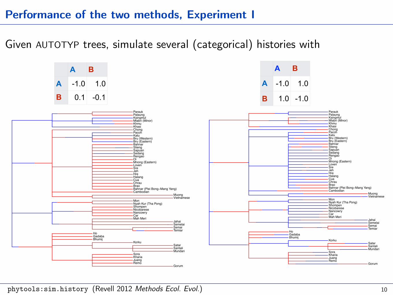
phytools:sim.history (Revell 2012 Methods Ecol. Evol.)
Performance of the two methods, Experiment I
Given AUTOTYP trees, simulate several (categorical) histories with
10
Gorum
Temiar
Car
Vietnamese
KhasiKhmu
Mundari
Semelai
Cambodian
Santali
Bahnar (Plei Bong−Mang Yang)
Remo
Brao
Bru (Eastern)Bru (Western)
Nyah Kur (Tha Pong)
ChrauCua
Bhumij
Nancowry
Gadaba
Halang
Ho
HreJeh
Jahai
Juang
Korku
Kharia
Sre
Katu
Loven
Mah Meri
Mnong (Eastern)
Mon
Mlabri (Minor)
Muong
Nicobarese
Oi
Pacoh
PalaungParauk
Ksingmul
Rengao
Semai
SedangSapuan
Sora
StiengBahnar
Satar
Shompen
Chong
A B
A -1.0 1.0
B 0.1 -0.1
A B
A -1.0 1.0
B 1.0 -1.0
Gorum
Temiar
Car
Vietnamese
KhasiKhmu
Mundari
Semelai
Cambodian
Santali
Bahnar (Plei Bong−Mang Yang)
Remo
Brao
Bru (Eastern)Bru (Western)
Nyah Kur (Tha Pong)
ChrauCua
Bhumij
Nancowry
Gadaba
Halang
Ho
HreJeh
Jahai
Juang
Korku
Kharia
Sre
Katu
Loven
Mah Meri
Mnong (Eastern)
Mon
Mlabri (Minor)
Muong
Nicobarese
Oi
Pacoh
PalaungParauk
Ksingmul
Rengao
Semai
SedangSapuan
Sora
StiengBahnar
Satar
Shompen
Chong
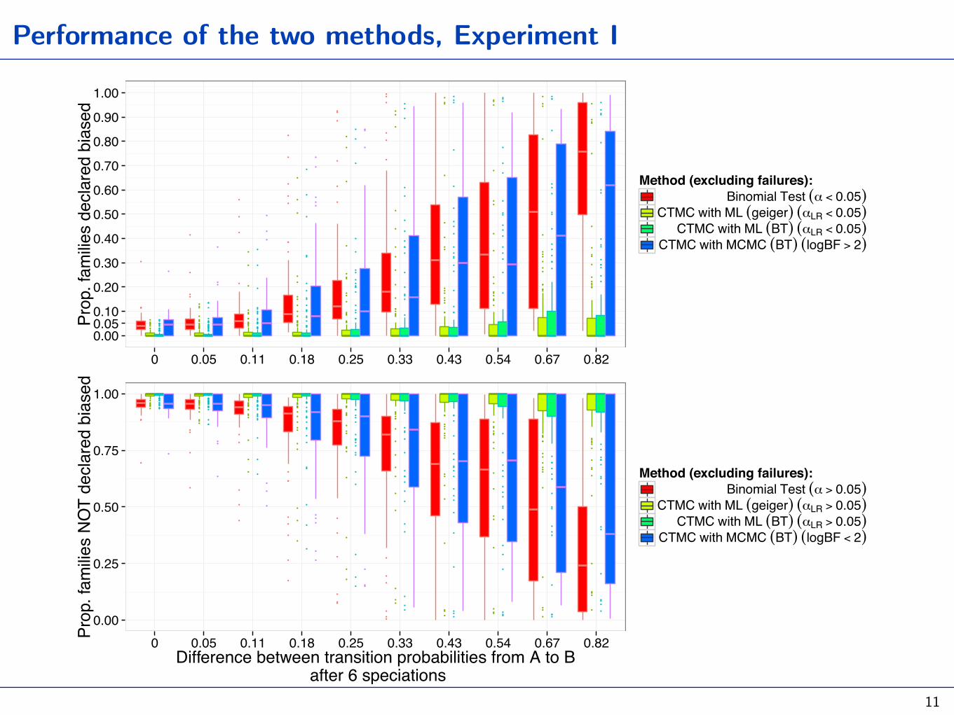
Performance of the two methods, Experiment I
11
●
●
●●
●
●●●●●
●
●
●●●●
●
●
●●
●
●●●
●
●
●
●
●
●
●
●
●●
●●
●●
●
●●
●
●●
●
●●
●
●
●●
●
●
●
●●●●
●
●●●●
●
●
●
●
●●
●●
●
●
●
●
●
●
●
●
●
●
●
●
●
●
●
●
●●
●
●
●
●
●
●
●
●
●
●
●
●
●
●
●
●●
●
●
●
●●
●
●
●
●
●
●
●
●
●
●
●
●
●
●
●●
●
●
●
●
●
●
●
●●
●
●
●
●
●
●
●●
●
●
●
●
●
●
●
●
●
●
●
●
●
●
●
●
●
●
●
●
●
●
●
●
●
●
●
●●
●
●
●
●
●
●
●
●
●
●
●
●
●
●
●
●
●
●
●
●
●
●
●
●
●
●●
●
●●
●
●
●
●
●
●
●
●
●
●
●
●
●
●
●
●
●
●
●
●●
●●
●
●
●
●
●
●
●
●
●
●
●
●
●
●
●
●
●
●
●
●
●
●
●
●
●
●
●
●
●
●
●●
●
●
●
●
●
●
●
●
●
●
●
●
●
●
●
●
●
●
●
●
●
●
●
●
●
●
●
●
●
●
●
●
●
●
●
●
●
●
●
●
●
●
●
●
●
●
●
●
●
●
●
●●●
●
●
●
●
●
●●
●
●
●
●
●
●
●
●
●
●
●
●
●
●
●
●●
●
●
●
●
●
●
●
●
●
●
●
●
●
●
●
●
●
●
●
●
●
●
●
●
●
●
●
●
●
●
●
●
●
●
●
●●
●
0.000.050.10
0.20
0.30
0.40
0.50
0.60
0.70
0.80
0.90
1.00
0 0.05 0.11 0.18 0.25 0.33 0.43 0.54 0.67 0.82
Prop
. fam
ilies
decl
ared
bia
sed
Method (excluding failures):Binomial Test (α < 0.05)
CTMC with ML (geiger) (αLR < 0.05)CTMC with ML (BT) (αLR < 0.05)
CTMC with MCMC (BT) (logBF > 2)
●
●
●●
●
●●●●●
●
●
●●●●
●
●
●●
●
●●●
●
●
●
●
●
●
●
●
●●
●●
●●
●
●●
●
●●
●
●●
●
●
●●
●
●
●
●●●●
●
●●●●
●
●
●
●
●●
●●
●
●
●
●
●
●
●
●
●
●
●
●
●
●
●
●
●
●●
●
●
●
●
●
●
●
●
●
●
●
●
●
●
●
●●
●
●
●
●●
●
●
●
●
●
●
●
●
●
●
●
●
●
●
●●
●
●
●
●
●
●
●
●●
●
●
●
●
●
●
●●
●
●
●
●
●
●
●
●
●
●
●
●
●
●
●
●
●
●
●
●
●
●
●
●
●
●
●
●●
●
●
●
●
●
●
●
●
●
●
●
●
●
●
●
●
●
●
●
●
●
●
●
●
●
●●
●
●●
●
●
●
●
●
●
●
●
●
●
●
●
●
●
●
●
●
●
●
●●
●●
●
●
●
●
●
●
●
●
●
●
●
●
●
●
●
●
●
●
●
●
●
●
●
●
●
●
●
●
●
●
●●
●
●
●
●
●
●
●
●
●
●
●
●
●
●
●
●
●
●
●
●
●
●
●
●
●
●
●
●
●
●
●
●
●
●
●
●
●
●
●
●
●
●
●
●
●
●
●
●
●
●
●
●●●
●
●
●
●
●
●●
●
●
●
●
●
●
●
●
●
●
●
●
●
●
●
●●
●
●
●
●
●
●
●
●
●
●
●
●
●
●
●
●
●
●
●
●
●
●
●
●
●
●
●
●
●
●
●
●
●
●
●
●●
●
0.00
0.25
0.50
0.75
1.00
0 0.05 0.11 0.18 0.25 0.33 0.43 0.54 0.67 0.82Difference between transition probabilities from A to B
after 6 speciations
Prop
. fam
ilies
NO
T de
clar
ed b
iase
d
Method (excluding failures):Binomial Test (α > 0.05)
CTMC with ML (geiger) (αLR > 0.05)CTMC with ML (BT) (αLR > 0.05)
CTMC with MCMC (BT) (logBF < 2)
Joint work in progress with Taras Zakharko
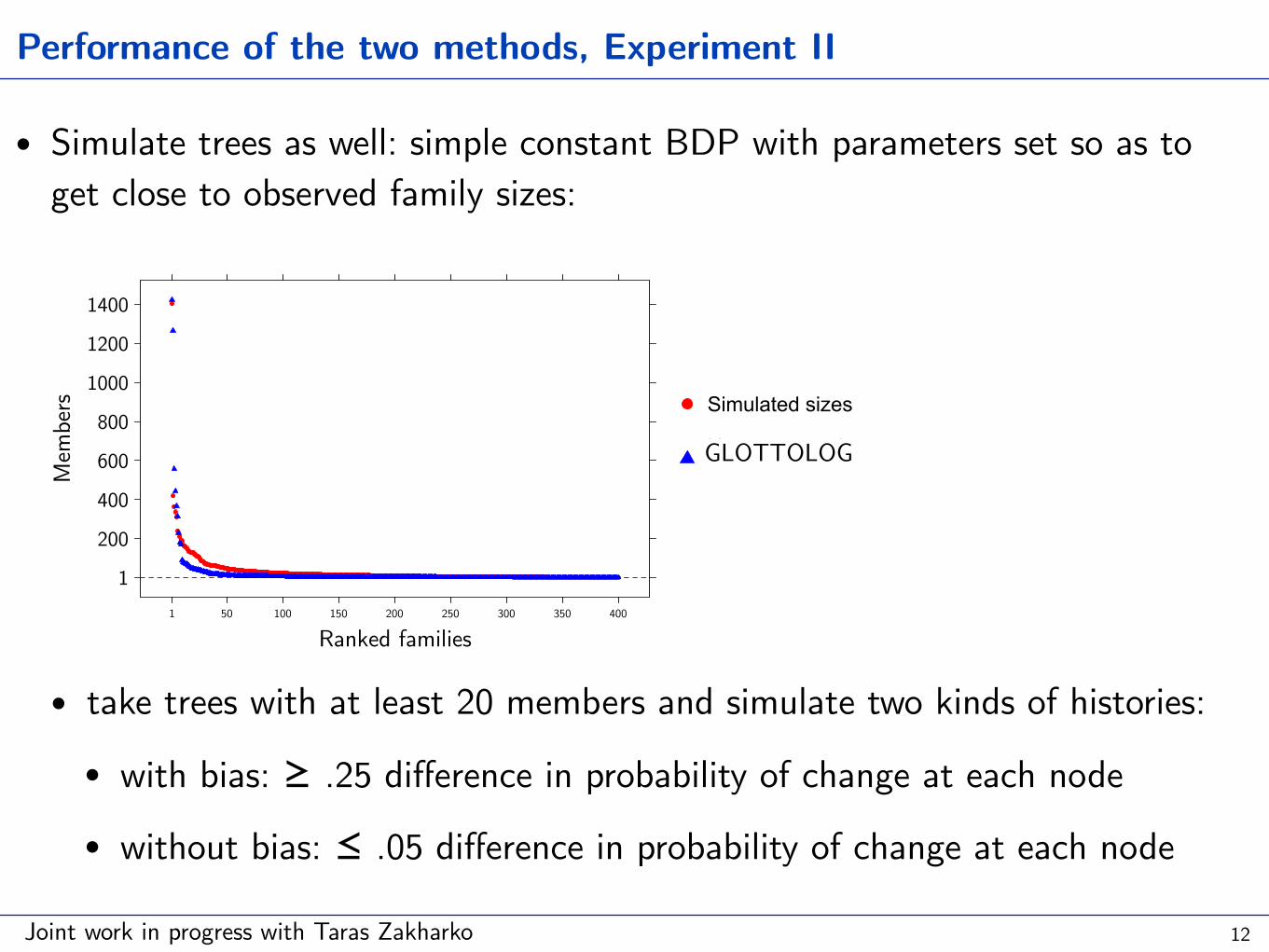
Performance of the two methods, Experiment II
• Simulate trees as well: simple constant BDP with parameters set so as to get close to observed family sizes:
• take trees with at least 20 members and simulate two kinds of histories:
• with bias: ≥ .25 difference in probability of change at each node
• without bias: ≤ .05 difference in probability of change at each node
12
Ranked families
Members
1200400600800100012001400
1 50 100 150 200 250 300 350 400
Simulated sizes
Hammarström'sclassificationGLOTTOLOG

Joint work in progress with Taras Zakharko
Performance of the two methods, Experiment II
13
0.0 0.2 0.4 0.6 0.8 1.0
01
23
45
Resulting proportion of languages per family with the same type
Density
10 steps (ca. 1000y)30 steps (ca. 3000y)50 steps (ca. 5000y)
0.0 0.2 0.4 0.6 0.8 1.0
01
23
Resulting proportion of languages per family with the same type
Density
10 steps (ca. 1000y)30 steps (ca. 3000y)50 steps (ca. 5000y)
without bias
with bias
Binomial tests
no bias detected bias detected
0.87 0.13
no bias detected bias detected
0.19 0.81
Bickel 2016 in Language Dispersals
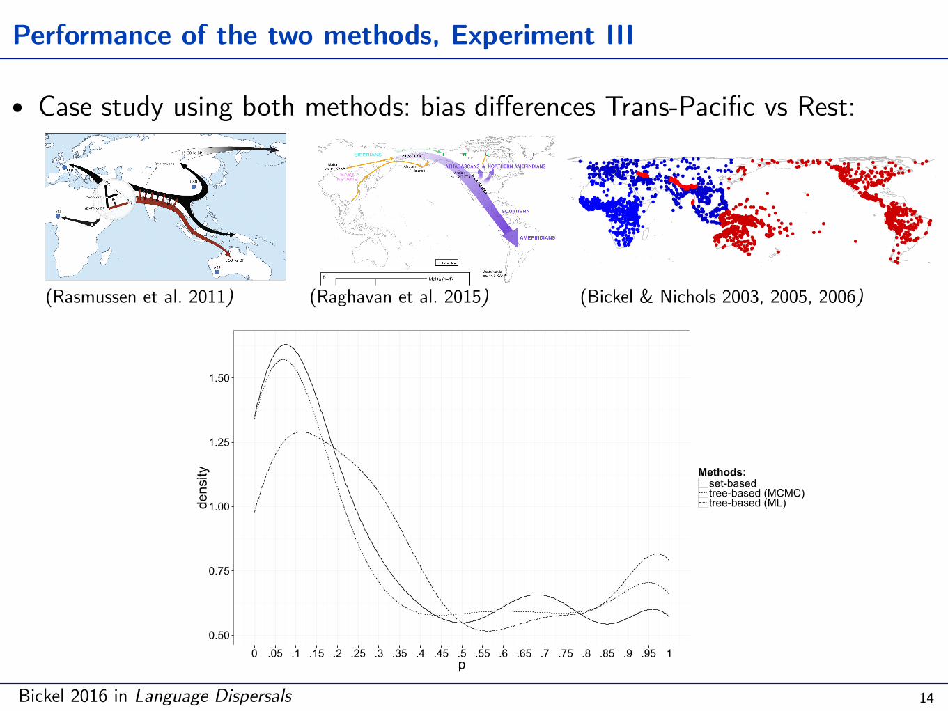
Performance of the two methods, Experiment III
• Case study using both methods: bias differences Trans-Pacific vs Rest:
14
0.50
0.75
1.00
1.25
1.50
0 .05 .1 .15 .2 .25 .3 .35 .4 .45 .5 .55 .6 .65 .7 .75 .8 .85 .9 .95 1p
density Methods:
set-basedtree-based (MCMC)tree-based (ML)
(Rasmussen et al. 2011)
had been genetically isolated from other pop-ulations (except possibly each other) since at least15,000 to 30,000 years B.P. (24).
To identify which model of human dispersalbest explains the data, we sequenced three HanChinese genomes to an average depth of 23 to24× (4) and used a test comparing the patterns ofsimilarity between these or the Aboriginal Aus-tralian to African and European individuals (4).This test, which we call D4P, is closely related totheD test (22, 23) but is far more robust to errorsand can detect subtle demographic signals in thedata that may be masked by large amounts ofsecondary gene flow (4).
Taking those sites where the Aboriginal Aus-tralian (ABR) differs from a Han Chinese repre-senting eastern Asia (ASN), and comparing ABRand ASN with the Centre d’Etude du Polymor-phisme Humain (CEPH) European sample (CEU)representing Europe and the Yoruba represent-ing Africa (YRI), the single-dispersal model (Fig.1A, top) predicts an equal number of sites sup-porting group 1 [(YRI, ASN), (CEU, ABR)] andgroup 2 [(YRI, ABR), (CEU, ASN)]. In contrast,the multiple-dispersal model (Fig. 1A, bottom)predicts an excess of group 2. Indeed, we founda statistically significant excess of sites (51.4%)grouping the Yoruba and Australian genomestogether (group 2) relative to the Yoruba and EastAsian genomes together (group 1, 48.6%, P <0.001), consistent with a basal divergence of Ab-original Australians in relation to East Asians andEuropeans (Table 2). Another possible explana-tion of our findings is that gene flow betweenmodern European and East Asian populationscaused these two populations to appear more sim-ilar to each other, generating an excess of sitesshowing group 2, even under the single-dispersal
model. However, simulations under such amodelshow that the amount of gene flow between Eu-ropeans and East Asians (5) cannot generate theexcess of sites showing group 2 unless Aborig-inal Australian, East Asian, and European ances-tral populations all split from each other aroundthe same time, with no subsequent migration be-tween aboriginal Australasians and East Asians(4). Such a model, however, would be incon-sistent with our results from D test, PCA, anddiscriminant analysis of principal components(DAPC) (4), given that the Aboriginal Australianis found to be genetically closer to East Asiansthan to Europeans (Table 1 and Fig. 1B). Thus,our findings suggest that a model in which Ab-original Australians are directly derived from an-cestral Asian populations, as proposed by thesingle-dispersal model, is not compatible withthe genomic data. Instead, our results favor themultiple-dispersal model in which the ancestorsof Aboriginal Australian and related popula-tions split from the Eurasian population beforeAsian and European populations split from eachother (4).
To estimate the times of divergence, we de-veloped a population genetic method for esti-mating demographic parameters from diploidwhole-genome data. The method uses patterns ofallele frequencies and linkage disequilibrium toobtain joint estimates of migration rates and di-vergence times between pairs of populations (4).Using this method, we estimate that aboriginalAustralasians split from the ancestral Eurasianpopulation 62,000 to 75,000 years B.P. This es-timate fits well with the mtDNA-based coales-cent estimates of 45,000 to 75,000 years B.P. ofthe non-African founder lineages (4, 15, 25, 26).Furthermore, we find that the European andAsian
populations split from each other only 25,000 to38,000 years B.P., in agreement with previousestimates (5, 6). All three populations, however,have a divergence time similar to the representa-tive African sequence. Additionally, our esti-mated split time between aboriginal Australasiansand the ancestral Eurasian population predicts theobserved excess of sites showing group 2 dis-cussed above (Table 2). To obtain confidenceintervals and test hypotheses, we used a blockbootstrap approach. In 100 bootstrap samples, wealways obtained a longer divergence time be-tween East Asians and the Aboriginal Australianthan between East Asians and Europeans, show-ing that we can reject the null hypothesis of atrichotomy in the population phylogeny with sta-tistical significance of approximately P < 0.01. Inthese analyses we have taken changes in popu-lation sizes and the effect of gene flow afterdivergence between populations into account.However, our models are still relatively simple,and the models we consider are only a subset ofall the possible models of human demography. Inaddition, we have not attempted directly tomodelthe combined effects of demography and selec-tion. The true history of human diversification islikely to be more complex than the simple de-mographic models considered here.
We used two approaches to test for admixturein the genomic sequence of the Aboriginal Aus-tralian with archaic humans [Neandertals andDenisovans (22, 23)]. We asked whether previ-ously identified high-confidence Neandertal ad-mixture segments in Europeans and Asians (22)could also be found in the Aboriginal Australian.We found that the proportion of such segmentsin the Aboriginal Australian closely matched thatobserved in European and Asian sequences (4).In the case of the Denisovans, we used a D test(22, 23) to search for evidence of admixture with-in the Aboriginal Australian genome. This testcompares the proportion of shared derived al-leles between an outgroup sequence (Denisovan)and two ingroup sequences. This test showed arelative increase in allele sharing between theDenisovan and the Aboriginal Australian genomes,compared to other Eurasians andAfricans includ-ing Andaman Islanders (4), but slightly less allelesharing than observed for Papuans. However, wefound that the D test is highly sensitive to errorsin the ingroup sequences (4), and shared errorsare of particular concern when the comparisonsinvolve both an ingroup and outgroup ancientDNA sequence. Althoughwe cannot exclude theseresults being influenced by such errors, the latterresult is consistent with the hypothesis of in-creased admixture betweenDenisovans or relatedgroups and the ancestors of the modern inhab-itants of Melanesia (23). This admixture mayhave occurred in Melanesia or, alternatively, inEurasia during the early migration wave.
The degree to which a single individual isrepresentative of the evolutionary history of Ab-original Australians more generally is unclear.Nonetheless, we conclude that the ancestors of
Fig. 2. Reconstruction of early spread of modern humans outside Africa. The tree shows the divergence ofthe Aboriginal Australian (ABR) relative to the CEPH European (CEU) and the Han Chinese (HAN) withgene flow between aboriginal Australasians and Asian ancestors. Purple arrow shows early spread of theancestors of Aboriginal Australians into eastern Asia ~62,000 to 75,000 years B.P. (ka BP), exchanginggenes with Denisovans, and reaching Australia ~50,000 years B.P. Black arrow shows spread of East Asians~25,000 to 38,000 years B.P. and admixing with remnants of the early dispersal (red arrow) some timebefore the split between Asians and Native American ancestors ~15,000 to 30,000 years B.P. YRI, Yoruba.
www.sciencemag.org SCIENCE VOL 334 7 OCTOBER 2011 97
REPORTS
on
Oct
ober
7, 2
011
www.
scie
ncem
ag.o
rgDo
wnlo
aded
from
Fig. 1. Origins and population history of Native Americans. (A) Our results show that the ancestors of all present-day Native Americans, including Amerindians and Athabascans, derived from a single migration wave into the Americas (purple), separate from the Inuit (green). This migration from East Asia occurred no later than 23 KYA and is in agreement with archaeological evidence from sites such as Monte Verde (50). A split between the northern and southern branches of Native Americans occurred ca. 13 KYA, with the former comprising Athabascans and northern Amerindians and the latter consisting of Amerindians in northern North America and Central and South America including the Anzick-1 individual (5). There is an admixture signal between Inuit and Athabascans and some northern Amerindians (yellow line); however, the gene flow direction is unresolved due to the complexity of the admixture events (28). Additionally, we see a weak signal related to Australo-Melanesians in some Native Americans, which may have been mediated through East Asians and Aleutian Islanders (yellow arrows). Also shown is the Mal’ta gene flow into Native American ancestors some 23 KYA (yellow arrow) (4). It is currently not possible for us to ascertain the exact geographical locations of the depicted events; hence, the positioning of the arrows should not be considered a reflection of these. B. Admixture plot created on the basis of TreeMix results (fig. S5) shows that all Native Americans form a clade, separate from the Inuit, with gene flow between some Native Americans and the North American Arctic. The number of genome-sequenced individuals included in the analysis is shown in brackets.
/ sciencemag.org/content/early/recent / 23 July 2015 / Page 15 / 10.1126/science.aab3884
(Raghavan et al. 2015) (Bickel & Nichols 2003, 2005, 2006)
Performance of the two methods: summary
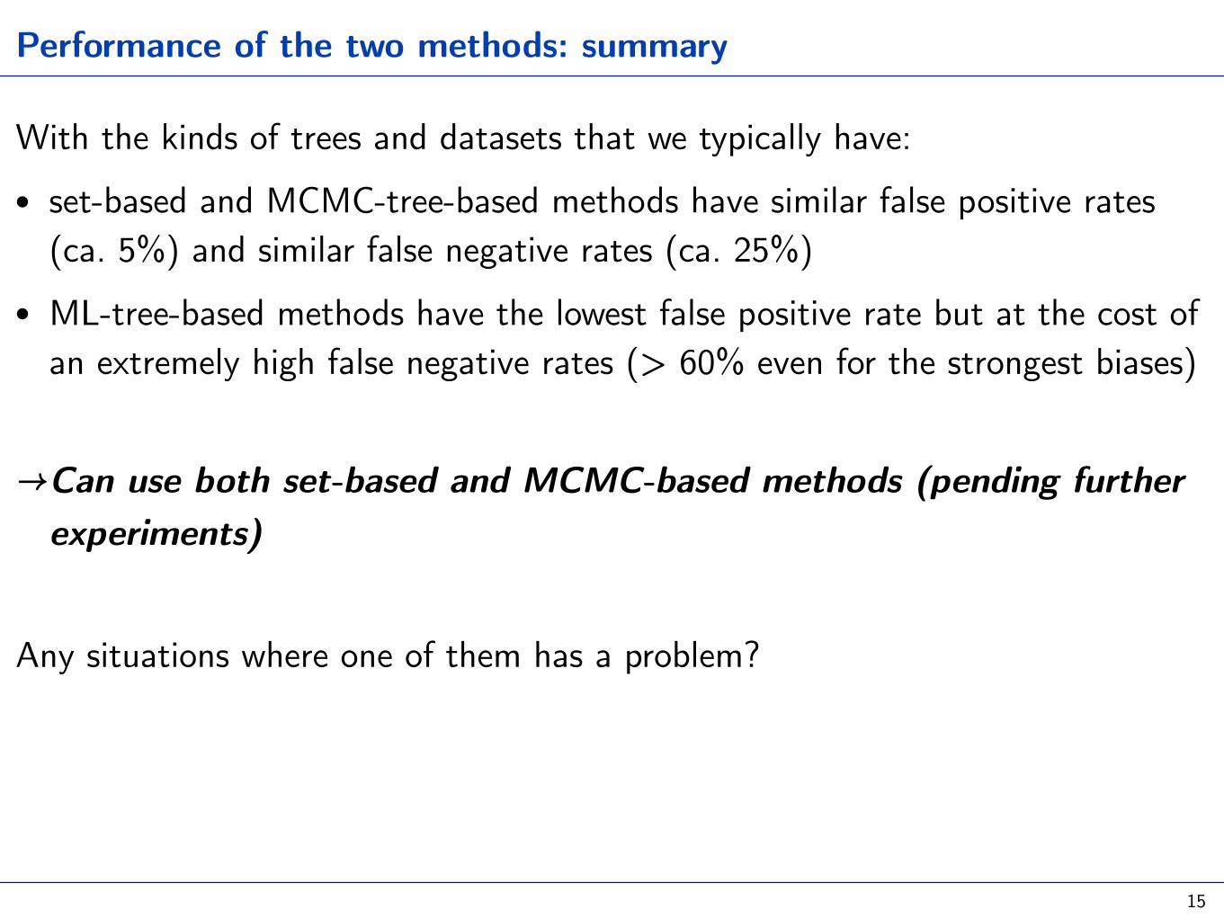
With the kinds of trees and datasets that we typically have: • set-based and MCMC-tree-based methods have similar false positive rates
(ca. 5%) and similar false negative rates (ca. 25%) • ML-tree-based methods have the lowest false positive rate but at the cost of
an extremely high false negative rates (> 60% even for the strongest biases)
→Can use both set-based and MCMC-based methods (pending further experiments)
Any situations where one of them has a problem?
15

Challenges for set-based methods: continuous data

Continuous variables
• Many numerical variables underlyingly discrete, e.g.
• Segment or tone inventories: add or loose an element or feature at a time
• Synthesis: add or loose a category at a time (e.g. grammaticalize an evidential, reanalyze a suffix as part of the stem)
• And in many cases, there are alternatives, e.g. trends in systems as continuous or discrete: Witzlack-Makarevich et al 2016 (cf before)
• but not always…
17
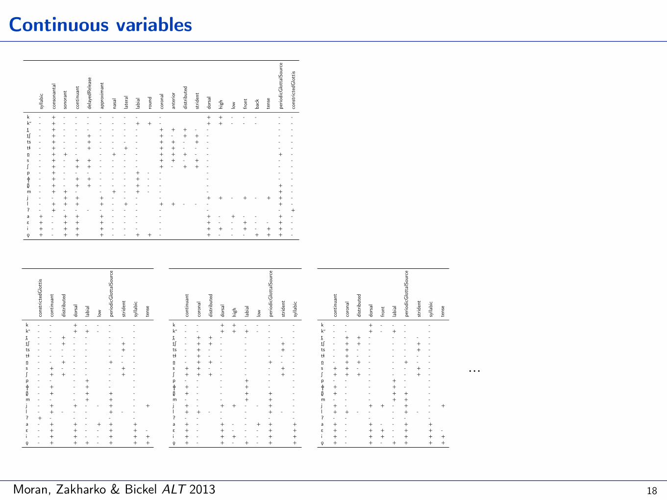
Moran, Zakharko & Bickel ALT 2013
Continuous variables
18
…

Continuous variables
A. set-based: presence of a given feature in all or any analyses? … not nice!
B. tree-based: prop. of analyses with a given feature → e.g. [coronal]:
19
●
●●
●
●●
●
●
●
●
●
●
●
●
●●
●
●
●
●
●
●
●
●
●
0.00
0.25
0.50
0.75
1.00
Aust
roas
iatic
Benu
e−Co
ngo
Chad
icCu
shitic
Drav
idia
n
East
ern
Cent
ral S
udan
icEa
ster
n Hi
ghla
nds
Eskim
o−Al
eut
Gur
Indo−E
urop
ean
Kwa
Mac
ro−G
eM
ande
Nilo
ticO
tom
angu
ean
Pano−T
acan
anQ
uech
uan
Salis
han
Sem
iticSe
pik
Sino−T
ibet
anTo
rrice
lliTu
pian
Turk
icUt
o−Az
teca
n
θ
OU fits better than BM:●
●
FALSETRUE
α●
●12

Challenges for tree-based methods: uniform data
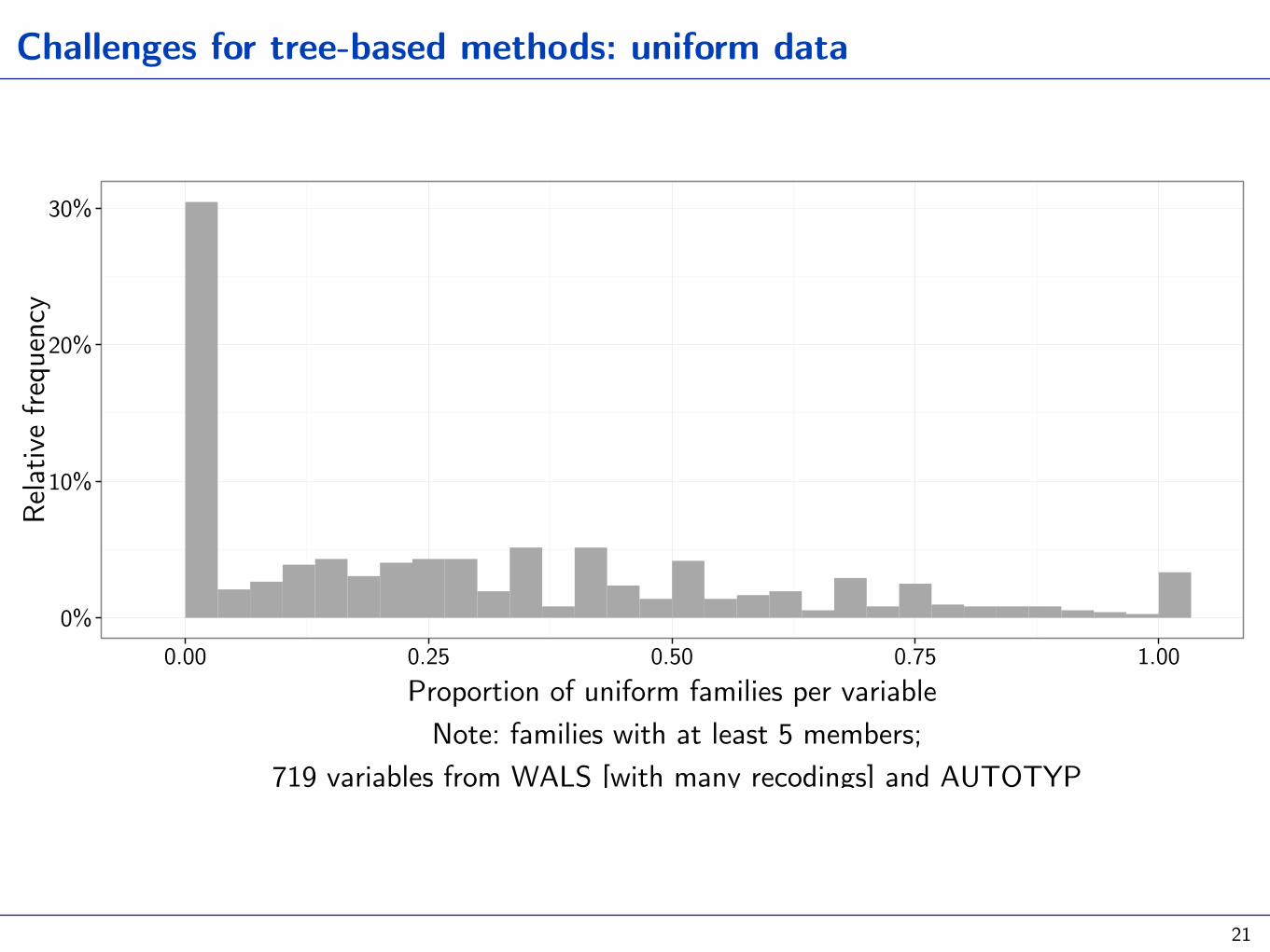
Challenges for tree-based methods: uniform data
21
0%
10%
20%
30%
0.00 0.25 0.50 0.75 1.00Proportion of uniform families per variable Note: families with at least 5 members;
719 variables from WALS [with many recodings] and AUTOTYP
Relat
ive fr
eque
ncy
Challenges for tree-based methods: split data

Bickel 2007 Ling Typ
Challenges for tree-based methods: split data (`multi-state’)
• Many typological data are problematic to aggregate at the language level, i.e. each language has multiple datapoints that are not just polymorphisms, dialect variants and the like (pace WALS)
• How do available methods handle this?
• A few examples first…
23

Multiple datapoint example I: grammatical relations
• Equivalence sets: S=A≠P, S≠A=P, S=P≠A etc. • Well-known splits:
• tense formation basis, e.g. ±based on participle; or ±PAST • aspect, e.g. ±perfective • main clause vs. dependent clause • person, e.g. S≠A in the first but S=A in the second and first person • lexical classes • co-arguments • etc.
24

Bickel 2015 Oxford Handbook of Ling Analysis, Witzlack-Makarevich & Bickel in prep
Multiple datapoint example I: grammatical relations
• Lexical classes, e.g. Hindi:
25
S
A P
A P
S
A P
A P
S
S
A P
A P
S
A P
A P
S

Witzlack-Makarevich & Bickel in prep
Multiple datapoint example I: grammatical relations
2626
participle-based
main
S=Atr=P
S=P≠Atr
S≠Atr=P
S≠Atr≠P
S=Atr≠P
not participle-based
S=Atr=P
S=P≠Atr
S≠Atr=PS≠Atr≠P
S=Atr≠P
depe
nden
t
S≠Atr≠P
S=Atr≠P
S≠Atr≠P
S=Atr≠P
Bickel 2015 Oxford Handbook of Ling Analysis, Witzlack-Makarevich & Bickel in prep
Multiple datapoint example I: grammatical relations
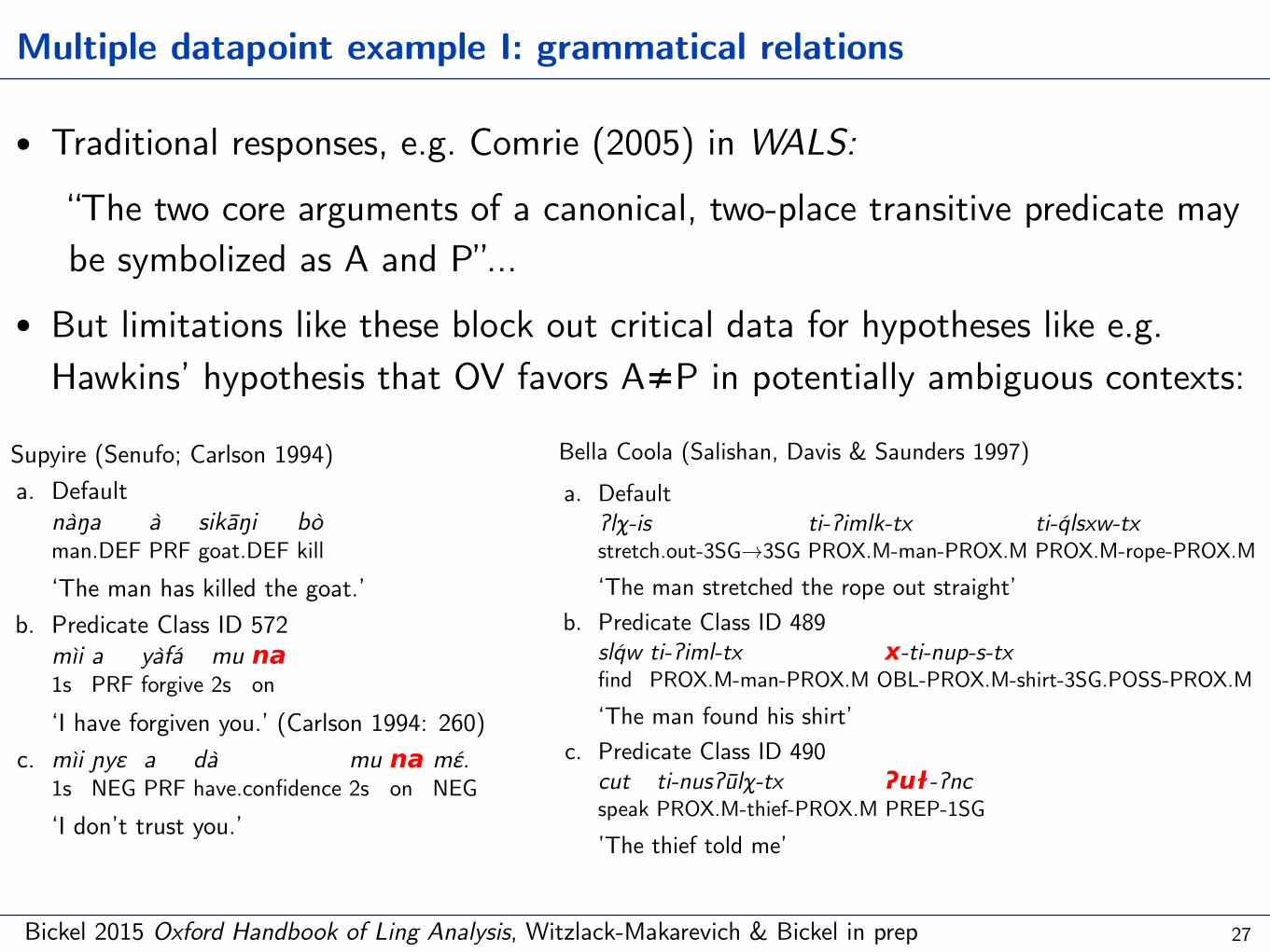
• Traditional responses, e.g. Comrie (2005) in WALS: “The two core arguments of a canonical, two-place transitive predicate may be symbolized as A and P”…
• But limitations like these block out critical data for hypotheses like e.g. Hawkins’ hypothesis that OV favors A≠P in potentially ambiguous contexts:
27
QD
QD
[
ɖXȭ
QD
QD
[
ɖXȭ

Witzlack-Makarevich, Zakharko, Bierkandt, Zúñiga & Bickel 2016 Linguistics
Multiple datapoint example I: grammatical relations
• Co-argument sensitivity, e.g. Ik:
28
7
co-occurs with all persons and in all roles. What occasionally blocks - i is two specific personfeature constellations: (i) if a first or third person acts on a second person, as in (8e) and (8f),dual number is not marked for the A argument, though it is marked for P arguments in thesame constellation, e.g. (8d); (ii) if an A argument acts on a third person i.e. if the third personis a P and not an S argument, as in (8g) and (8h), dual is not marked for P arguments, though itis marked for A arguments, cf. (8c).
e presence of dual marking in Belhare can only be captured by appeal to the referentialfeatures of two arguments at once; the pa ern cannot be analyzed in terms of a referentialhierarchy: condition (i) cannot be re-cast as a statement like ‘all A arguments lower than thesecond person on a 1/2 ≻ 3 hierarchy’ because in other scenarios low-ranking persons do allowdual marking in A role, e.g. the third person in (8c). Condition (ii) does amount to a constrainton what can be thought of as the lowest segment of the hierarchy, i.e. all third persons. But itonly holds of P arguments, and does not generalize across all third persons. is is differentfrom hierarchical agreement of the kind that is known from the Emerillon or Plains Cree prefixmarking pa erns discussed above.
Co-argument sensitivity that is not based on a hierarchy is also found with case marking.is can be illustrated by the following examples from Ik. In Ik, the P argument can be either
in the nominative, as in (9a) and (9b), or in the accusative case, as in (9c) and (9d):
(9) Ik (Kuliak, Uganda; König 2009)
a. en-í-asee-1s-A
nk-aI-NOM
wík-a.children-NOM
‘I see the children.’
b. en-es-íd-asee-IRR-2s-A
bi-ayou-NOM
wík-a.children-NOM
‘You (sg) will see the children.’
c. en-es-uɠot-asee-IRR-AND-A
wík-áchildren-NOM
njíní-ka.1pINCL-ACC
‘ e children will see us (incl.).’
d. en-es-át-asee-IRR-3p-A
ńt-athey-NOM
ceki-ka.woman-ACC
‘ ey will see the woman.’
What determines the distribution of the case markers on the P argument is the nature of theA arguments: the P argument is in the accusative case only if the A argument is third person,otherwise the P argument is in the nominative case. is is made explicit in Table 1, wheresubscripted numbers indicate person (e.g. S1 refers to the first person S argument).
Similar to Belhare and in contrast to the Emerillon or Tagalog examples, it is impossibleto account for differential P marking here by formulating a referential hierarchy of any kind,whereas the reference to the nature of co-arguments is unavoidable. For example, one couldconsider an analysis of Ik based on a hierarchy that ranks first and second person above thirdperson (1/2 ≻ 3). en, if the P argument is higher or equal to the A argument on this hierar-chy, it is in the accusative case. is hierarchy would correctly predict the distribution of theaccusative and nominative cases in the scenarios involving third persons, but it would overgen-erate in that the analysis would also predict the accusative P argument in scenarios involvingonly first and second person (‘local’ scenarios).
e examples from Belhare and Ik show that for some systems of case and agreement mark-ing it is unavoidable to make reference to specific constellations of person features. In principle,however, it seems that reference to such constellations is not fundamentally different from ref-erence to single referential properties. Reference to single referential properties is something
DRAFT – February 17, 2015
10
Comparative triads Alignment
S argument A argument withits co-argument
P argument withits co-argument
S1 A1 [with P2] P1 [with A2] neutral
S1 A1 [with P2] P1 [with A3] accusative
S1 A1 [with P3] P1 [with A2] neutral
S1 A1 [with P3] P1 [with A3] accusative
S2 A2 [with P1] P2 [with A1] neutral
S2 A2 [with P1] P2 [with A3] accusative
S2 A2 [with P3] P2 [with A1] neutral
S2 A2 [with P3] P2 [with A3] accusative
S3 A3 [with P1] P3 [with A1] neutral
S3 A3 [with P1] P3 [with A2] neutral
S3 A3 [with P1] P3 [with A3] accusative
S3 A3 [with P2] P3 [with A1] neutral
S3 A3 [with P2] P3 [with A2] neutral
S3 A3 [with P2] P3 [with A3] accusative
S3 A3 [with P3] P3 [with A1] neutral
S3 A3 [with P3] P3 [with A2] neutral
S3 A3 [with P3] P3 [with A3] accusative
Table 2: Comparison triads for determining alignment of Ik case marking
DRAFT – February 17, 2015
Multiple datapoint example I: grammatical relations
29
A=P
A≠P
A=P
A≠P
A=P
A≠P
A=P
A=P
A=P
A≠P
A=P

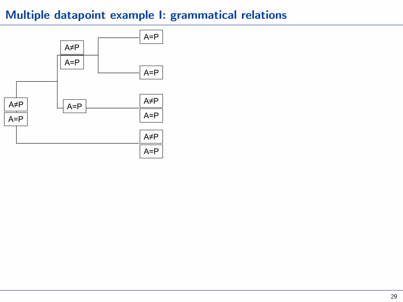
Multiple datapoint example I: grammatical relations
A. Set-based method: the distribution among tips as the result of many binomial trials (gain vs loose a predicate class with case)
30
A=P
A≠P
A=P
A≠P
A=P
A≠P
A=P
A=P
A=P
A≠P
A=P
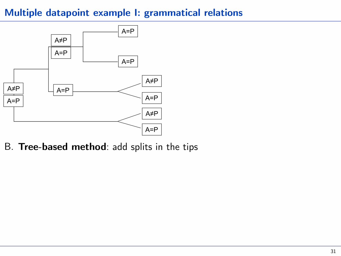
Multiple datapoint example I: grammatical relations
B. Tree-based method: add splits in the tips
31
A=P
A≠P
A=P
A≠P
A=P
A≠P
A=P
A=P
A=P
A≠P
A=P
Bickel, Choudhary, Witzlack-Makarevich, Schlesewsky & Bornkessel-Schlesewsky 2015 PLOS ONE
How can we work with such data?
32
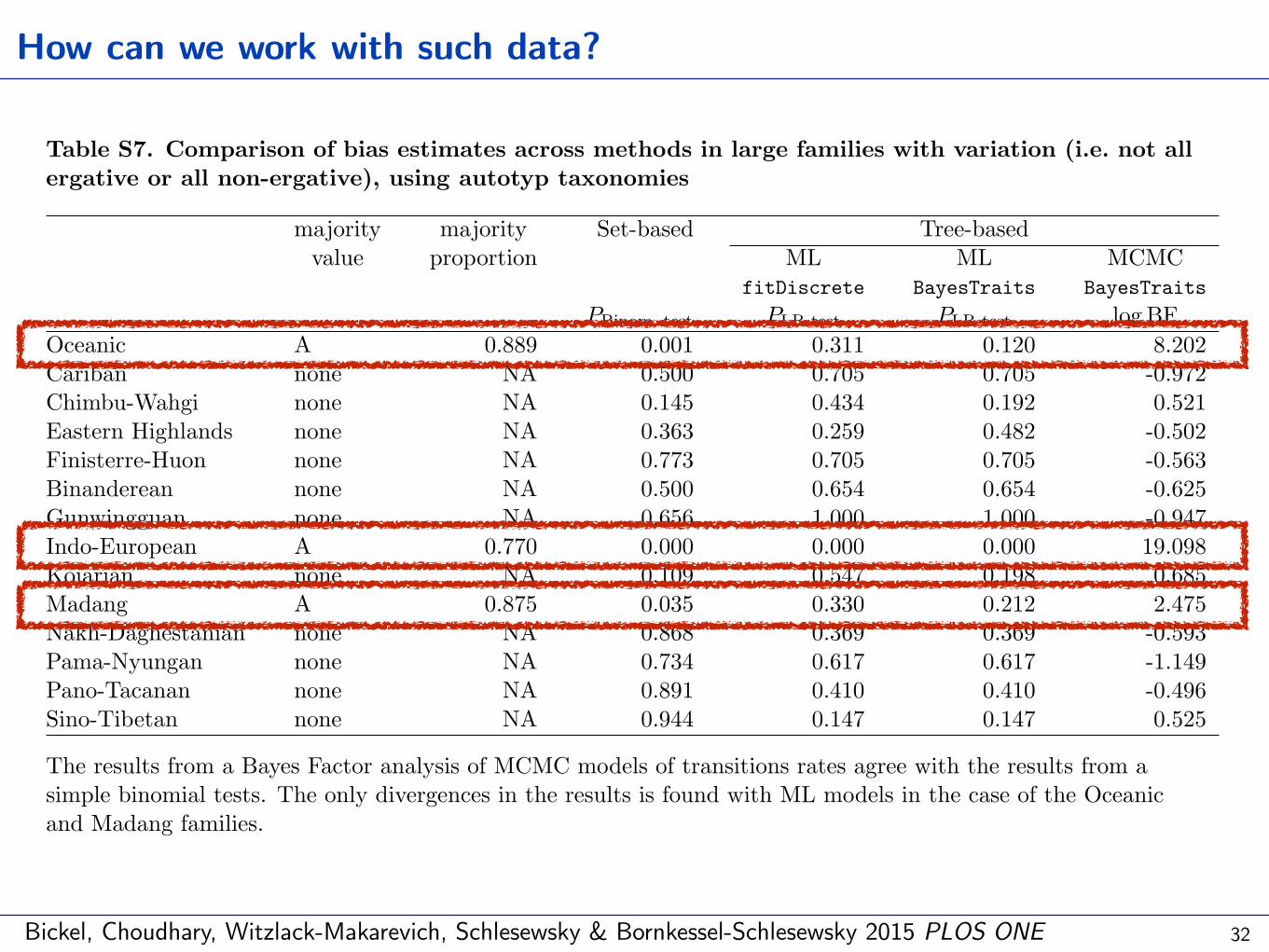
Table S7. Comparison of bias estimates across methods in large families with variation (i.e. not allergative or all non-ergative), using autotyp taxonomies
majority majority Set-based Tree-basedvalue proportion ML ML MCMC
fitDiscrete BayesTraits BayesTraits
PBinom. test PLR test PLR test log BFOceanic A 0.889 0.001 0.311 0.120 8.202Cariban none NA 0.500 0.705 0.705 -0.972Chimbu-Wahgi none NA 0.145 0.434 0.192 0.521Eastern Highlands none NA 0.363 0.259 0.482 -0.502Finisterre-Huon none NA 0.773 0.705 0.705 -0.563Binanderean none NA 0.500 0.654 0.654 -0.625Gunwingguan none NA 0.656 1.000 1.000 -0.947Indo-European A 0.770 0.000 0.000 0.000 19.098Koiarian none NA 0.109 0.547 0.198 0.685Madang A 0.875 0.035 0.330 0.212 2.475Nakh-Daghestanian none NA 0.868 0.369 0.369 -0.593Pama-Nyungan none NA 0.734 0.617 0.617 -1.149Pano-Tacanan none NA 0.891 0.410 0.410 -0.496Sino-Tibetan none NA 0.944 0.147 0.147 0.525
The results from a Bayes Factor analysis of MCMC models of transitions rates agree with the results from asimple binomial tests. The only divergences in the results is found with ML models in the case of the Oceanicand Madang families.
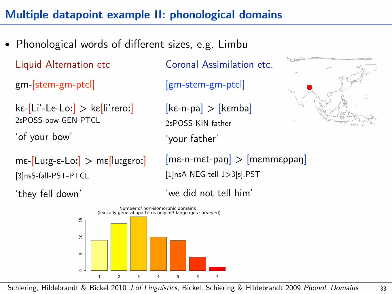
1 2 3 4 5 6 7
Number of non-isomorphic domains (lexically general ppatterns only, 63 languages surveyed)
05
10
15
Schiering, Hildebrandt & Bickel 2010 J of Linguistics; Bickel, Schiering & Hildebrandt 2009 Phonol. Domains
Multiple datapoint example II: phonological domains
• Phonological words of different sizes, e.g. Limbu
33
Liquid Alternation etc
gm-[stem-gm-ptcl]
kɛ-[Li’-Le-Loː] > kɛ[li’reroː] 2sPOSS-bow-GEN-PTCL
‘of your bow’
mɛ-[Luːg-ɛ-Loː] > mɛ[luːgɛroː] [3]nsS-fall-PST-PTCL
‘they fell down’
Coronal Assimilation etc.
[gm-stem-gm-ptcl]
[kɛ-n-pa] > [kɛmba] 2sPOSS-KIN-father
‘your father’
[mɛ-n-mɛt-paŋ] > [mɛmmɛppaŋ] [1]nsA-NEG-tell-1>3[s].PST
‘we did not tell him’
Bickel, Schiering & Hildebrandt 2009 in Phonol. Domains
Multiple datapoint example II: phonological domains
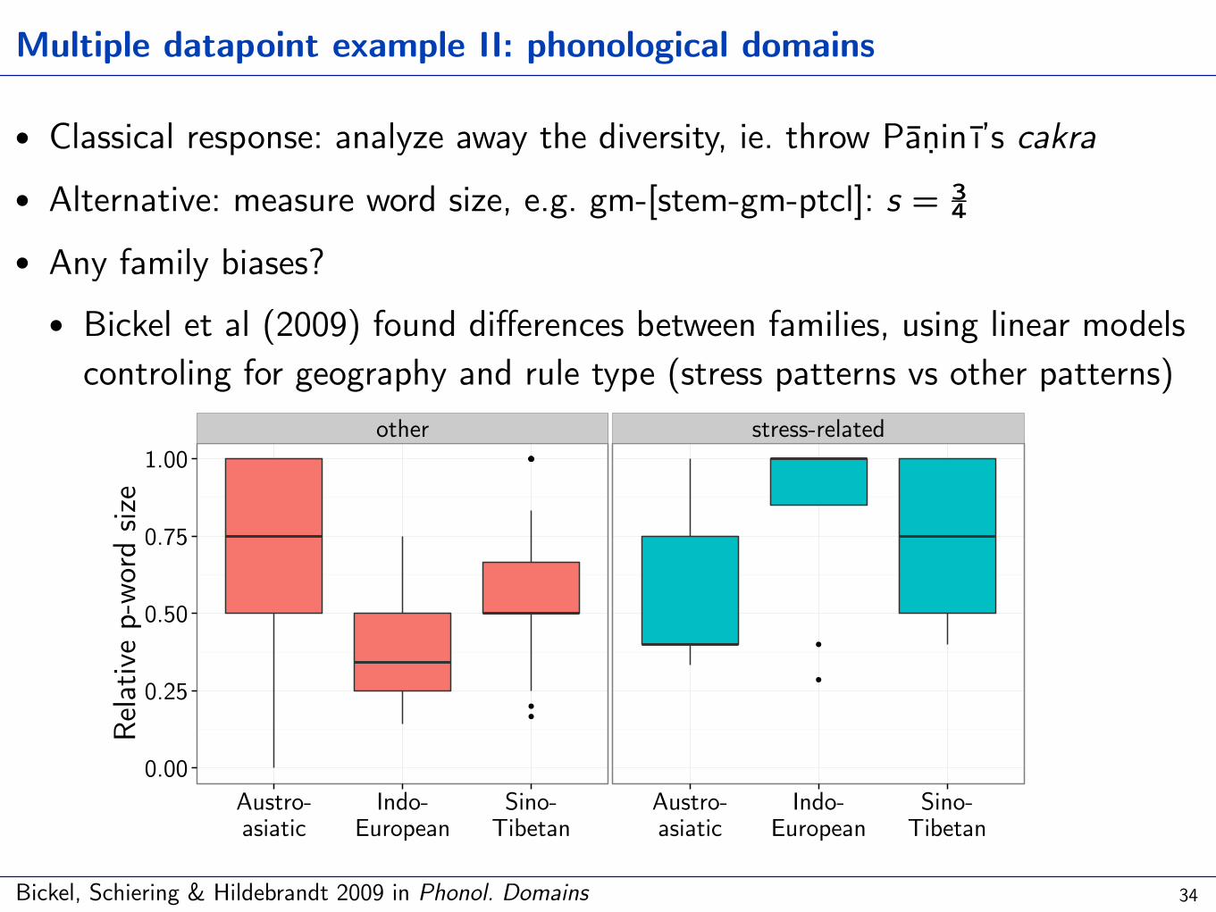
• Classical response: analyze away the diversity, ie. throw Pāṇinī’s cakra • Alternative: measure word size, e.g. gm-[stem-gm-ptcl]: s = ¾ • Any family biases?
• Bickel et al (2009) found differences between families, using linear models controling for geography and rule type (stress patterns vs other patterns)
34
other stress-related
0.00
0.25
0.50
0.75
1.00
Austro-asiatic
Indo-European
Sino-Tibetan
Austro-asiatic
Indo-European
Sino-Tibetan
Relat
ive p
-wor
d siz
e

Multiple datapoint example II: phonological domains
• But individual biases? — no easy way with set-based methods • Tree-based method: compare Brownian Motion vs. Ornstein-Uhlenbeck m.
35
Car
Vietnamese
Khasi
Khmu
Semelai
Cambodian
Santali
Chrau
Jahai
Kharia
Mon
Pacoh
Armenian (Eastern)
French (colloquial)
German
HindiNepali
Irish
Persian
Greek (modern)
Spanish
Armenian (Western)
Swedish
Romani (Sepecides)
Czech
Dutch
LithuanianPolish
Belhare
Mandarin
BurmeseNewar (Dolakha)
MeitheiGaro
Kayah LiKinnauri
Hayu
ApataniKham
Limbu
ManangeTibetan (Lhasa)Tibetan (Kyirong)
QiangTibetan (Dege)
WuCantonese
Rabha
Austroasiatic Indo-European Sino-Tibetan
No evidence for bias pLR = .22
Evidence for bias pLR < .001 θ = .39 α = .81
Evidence for bias pLR < .001 θ = .57 α = .71

Challenges for all methods: isolates and small families
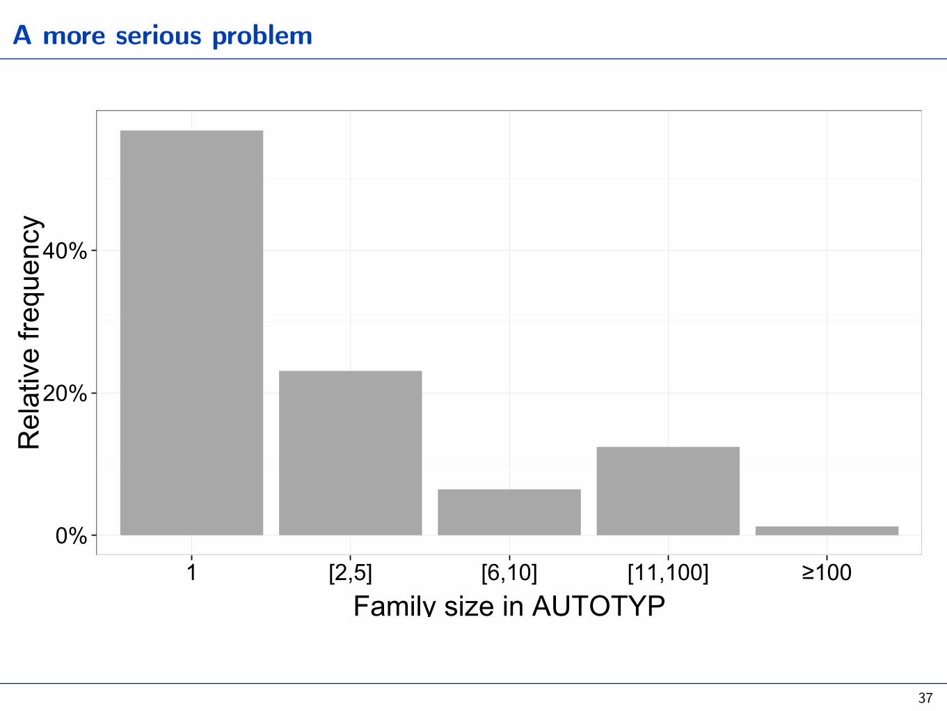
A more serious problem
37
0%
20%
40%
1 [2,5] [6,10] [11,100] ≥100Family size in AUTOTYP
Rel
ativ
e fre
quen
cy
Bickel 2011 Ling Typ, 2013 Lang Typ and Hist Cont
Estimate bias probabilities behind small families and isolates
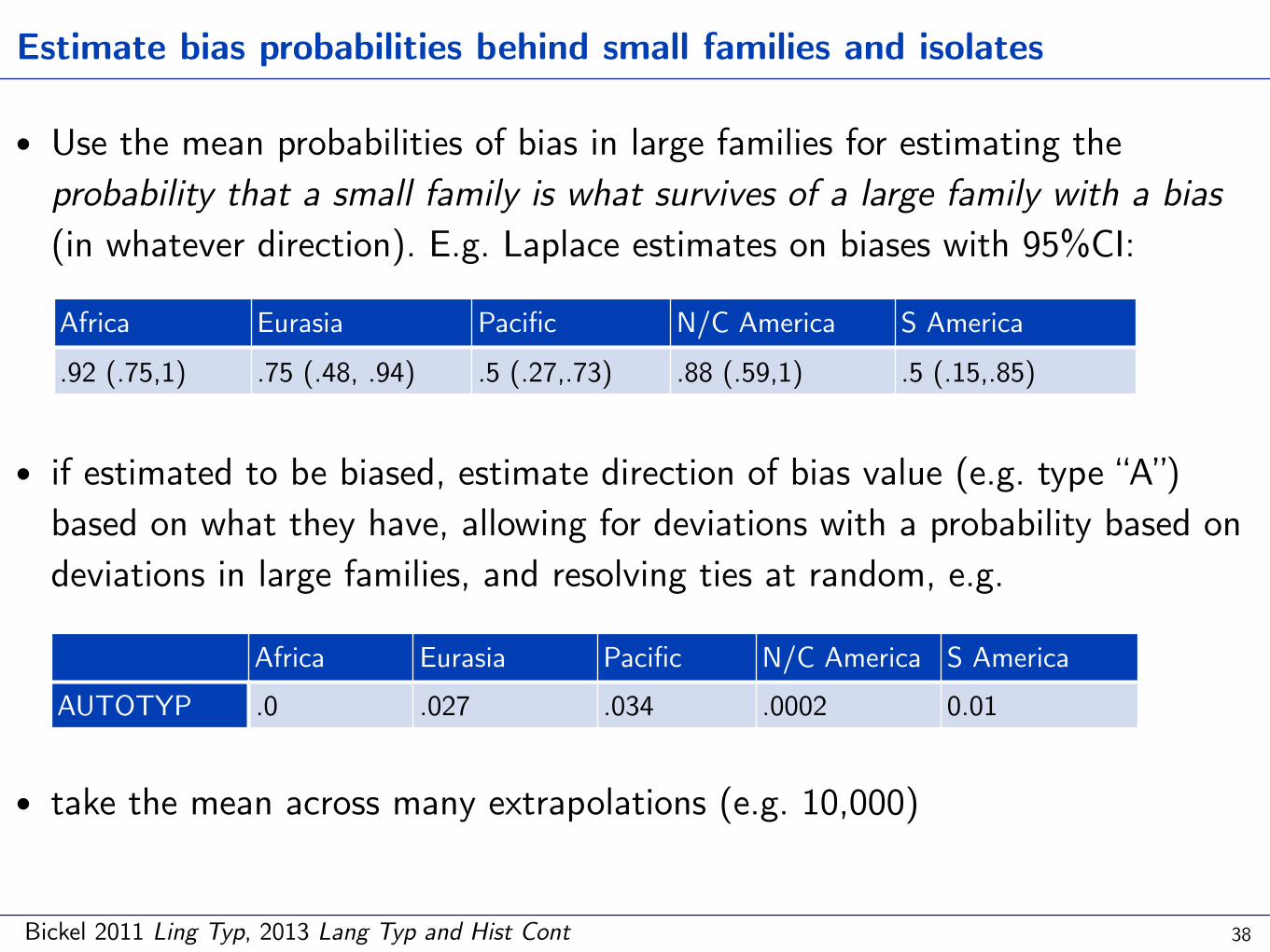
• Use the mean probabilities of bias in large families for estimating the probability that a small family is what survives of a large family with a bias (in whatever direction). E.g. Laplace estimates on biases with 95%CI:
• if estimated to be biased, estimate direction of bias value (e.g. type “A”) based on what they have, allowing for deviations with a probability based on deviations in large families, and resolving ties at random, e.g.
• take the mean across many extrapolations (e.g. 10,000)
38
Africa Eurasia Pacific N/C America S America.92 (.75,1) .75 (.48, .94) .5 (.27,.73) .88 (.59,1) .5 (.15,.85)
Africa Eurasia Pacific N/C America S AmericaAUTOTYP .0 .027 .034 .0002 0.01
Joint work in progress with Taras Zakharko
Estimate bias probabilities behind small families and isolates
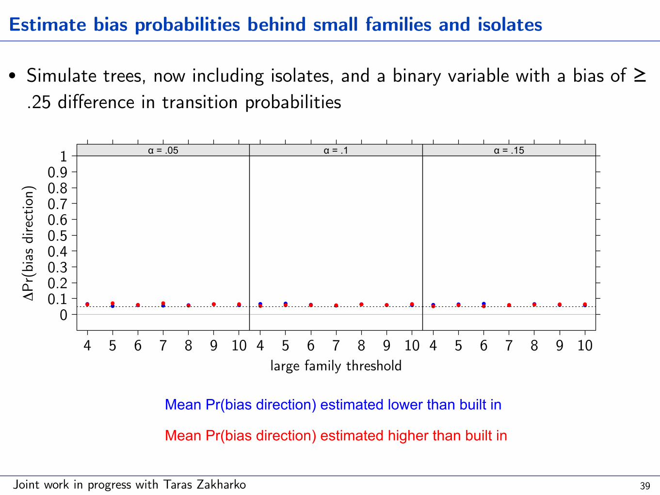
• Simulate trees, now including isolates, and a binary variable with a bias of ≥ .25 difference in transition probabilities
39
large family threshold
ΔPr
(bias
dire
ction
)
00.10.20.30.40.50.60.70.80.91
4 5 6 7 8 9 10
α = .05
4 5 6 7 8 9 10
α = .1
4 5 6 7 8 9 10
α = .15
Mean Pr(bias direction) estimated lower than built in
Mean Pr(bias direction) estimated higher than built in

Conclusions
• Family biases can be reasonably well estimated with set-based methods,
• except for continuous traits
• Family biases can be reasonably well estimated with MCMC tree-based methods,
• except when data is uniform (and for 70% variables, some families are uniform!)
• except when data is split (but the methods seem relatively robust here)
• The biggest challenge for all methods: isolates and small families (ca. 70% of families!)
‣ extrapolation method in https://github.com/IVS-UZH/familybias
40


![[Edu.joshuatly.com] Pahang JUJ SPM 2011 Chemistry](https://static.documents.pub/doc/80x56/577cc1071a28aba711920196/edujoshuatlycom-pahang-juj-spm-2011-chemistry.jpg)

![Physics JUJ 2009 [Edu.joshuatly.com]](https://static.documents.pub/doc/80x56/563dbfa0550346aa9ab0c1b2/physics-juj-2009-edujoshuatlycom.jpg)
