

Draft version September 12, 2021Typeset using LATEX twocolumn style in AASTeX63
Molecules with ALMA at Planet-forming Scales. XX. The Massive Disk Around GM Aurigae
Kamber R. Schwarz ,1, 2, ∗ Jenny K. Calahan ,3 Ke Zhang ,4, 3, † Felipe Alarcon ,3 Yuri Aikawa ,5
Sean M. Andrews ,6 Jaehan Bae ,7, 8, ∗ Edwin A. Bergin ,3 Alice S. Booth ,9, 10 Arthur D. Bosman ,3
Gianni Cataldi ,11, 5 L. Ilsedore Cleeves ,12 Ian Czekala ,13, 14, 15, 16, 17 Jane Huang ,3, ∗ John D. Ilee ,18
Charles J. Law ,6 Romane Le Gal ,6, 19, 20, 21 Yao Liu ,22 Feng Long ,6 Ryan A. Loomis ,23
Enrique Macıas ,24, 25 Melissa McClure ,9 Francois Menard ,26 Karin I. Oberg ,6 Richard Teague ,6
Ewine van Dishoeck ,9 Catherine Walsh ,10 and David J. Wilner 6
1Lunar and Planetary Laboratory, University of Arizona, 1629 E. University Blvd, Tucson, AZ 85721, USA2Max-Planck-Institut fur Astronomie, Konigstuhl 17, 69117 Heidel- berg, Germany
3Department of Astronomy, University of Michigan, 323 West Hall, 1085 South University Avenue, Ann Arbor, MI 48109, USA4Department of Astronomy, University of Wisconsin-Madison, 475 N Charter St, Madison, WI 53706
5Department of Astronomy, Graduate School of Science, The University of Tokyo, Tokyo 113-0033, Japan6Center for Astrophysics | Harvard & Smithsonian, 60 Garden St., Cambridge, MA 02138, USA
7Earth and Planets Laboratory, Carnegie Institution for Science, 5241 Broad Branch Road NW, Washington, DC 20015, USA8Department of Astronomy, University of Florida, Gainesville, FL 32611, USA
9Leiden Observatory, Leiden University, 2300 RA Leiden, the Netherlands10School of Physics and Astronomy, University of Leeds, Leeds, UK, LS2 9JT
11National Astronomical Observatory of Japan, Osawa 2-21-1, Mitaka, Tokyo 181-8588, Japan12Department of Astronomy, University of Virginia, 530 McCormick Rd, Charlottesville, VA 22904
13Department of Astronomy and Astrophysics, 525 Davey Laboratory, The Pennsylvania State University, University Park, PA 16802,USA
14Center for Exoplanets and Habitable Worlds, 525 Davey Laboratory, The Pennsylvania State University, University Park, PA 16802,USA
15Center for Astrostatistics, 525 Davey Laboratory, The Pennsylvania State University, University Park, PA 16802, USA16Institute for Computational & Data Sciences, The Pennsylvania State University, University Park, PA 16802, USA
17Department of Astronomy, 501 Campbell Hall, University of California, Berkeley, CA 94720-3411, USA∗
18School of Physics & Astronomy, University of Leeds, Leeds LS2 9JT, UK19IRAP, Universite de Toulouse, CNRS, CNES, UT3, Toulouse, France
20IPAG, Universite Grenoble Alpes, CNRS, IPAG, F-38000 Grenoble, France21IRAM, 300 rue de la piscine, F-38406 Saint-Martin d’Heres, France
22Purple Mountain Observatory & Key Laboratory for Radio Astronomy, Chinese Academy of Sciences, Nanjing 210023, China23National Radio Astronomy Observatory, 520 Edgemont Rd., Charlottesville, VA 22903, USA
24Joint ALMA Observatory, Avenida Alonso de Cordova 3107, Vitacura, Santiago, Chile25European Southern Observatory, Avenida Alonso de Cordova 3107, Vitacura, Santiago, Chile
26Univ. Grenoble Alpes, CNRS, IPAG, F-38000 Grenoble, France
(Received; Revised September 12, 2021; Accepted)
Submitted to AJ
ABSTRACT
Gas mass remains one of the most difficult protoplanetary disk properties to constrain. With much
of the protoplanetary disk too cold for the main gas constituent, H2, to emit, alternative tracers such
as dust, CO, or the H2 isotopolog HD are used. However, relying on disk mass measurements from any
single tracer requires assumptions about the tracer’s abundance relative to H2 and the disk temperature
structure. Using new Atacama Large Millimeter/submillimeter Array (ALMA) observations from the
Molecules with ALMA at Planet-forming Scales (MAPS) ALMA Large Program as well as archival
Corresponding author: Kamber R. Schwarz

2 Schwarz et al.
ALMA observations, we construct a disk physical/chemical model of the protoplanetary disk GM
Aur. Our model is in good agreement with the spatially resolved CO isotopolog emission from eleven
rotational transitions with spatial resolution ranging from 0.15′′ to 0.46′′(24-73 au at 159 pc) and
the spatially unresolved HD J = 1 − 0 detection from Herschel. Our best-fit model favors a cold
protoplanetary disk with a total gas mass of approximately 0.2 M, a factor of 10 reduction in CO gas
inside roughly 100 au and a factor of 100 reduction outside of 100 au. Despite its large mass, the disk
appears to be on the whole gravitationally stable based on the derived Toomre Q parameter. However,
the region between 70 and 100 au, corresponding to one of the millimeter dust rings, is close to being
unstable based on the calculated Toomre Q of < 1.7. This paper is part of the MAPS special issue of
the Astrophysical Journal Supplement.
Keywords: Astrochemistry
1. INTRODUCTION
Protoplanetary disk mass is a fundamental property
influencing virtually all aspects of the disk’s evolution
and the resulting planetary system. It sets a limit on
the mass available to forming planets and determines
the mechanisms that shape the final system architec-
ture. Gravitational instability (GI) in a protoplanetary
disk can result in the formation of massive companions
at separations of hundreds of astronomical units from
the central star (Boss 1997). Gravitational collapse at
early stages results in the formation of close multiple-
star systems (Tobin et al. 2018). In other cases, GI can
result in the formation of massive planets at wide sep-
aration, such as the giant planets proposed to exist in
the HD 163296 disk (Isella et al. 2016; Liu et al. 2018;
Pinte et al. 2018; Teague et al. 2018).
In a recent study of the HD 163296 system, Booth
et al. (2019) found a total disk mass of 0.31 M based on
observations of the optically thin CO isotopolog 13C17O.
They further found that the disk currently is stable
against gravitational collapse, though they noted the
disk may have been more massive, and thus unstable,
in the past, having had ample time to accrete mass onto
the central star. Analysis of the HL Tau disk using the
same 13C17O transition indicates this much younger sys-
tem surrounded by a residual envelope has a lower total
disk mass of 0.2 M but is likely unstable at radii from
50-110 au (Booth & Ilee 2020), spanning several of the
rings and dark bands observed in the millimeter contin-
uum (ALMA Partnership et al. 2015).
Disk gas mass remains one of the most difficult pa-
rameters to constrain. This is because the dominant
gas component, H2, does not readily emit throughout
most of the disk due to its lack of a permanent dipole
moment. Instead, trace species such as CO and dust are
∗ NASA Hubble Fellowship Program Sagan Fellow† NASA Hubble Fellow
used to extrapolate to a total gas mass. However, each
tracer relies on assumptions that may not be applicable
to protoplanetary disks (see Bergin & Williams (2017)
for a review).
Converting dust continuum emission to a total dust
mass requires assumptions about the grain size distri-
bution, dust composition, scattering, and dust temper-
ature. The dust mass is often then converted to a gas
mass assuming a gas-to-dust mass ratio of 100, as mea-
sured for the interstellar medium (ISM). However, sev-
eral processes can change the derived ratio, including
differential radial drift for grains of different sizes, dust
growth beyond the observable range, accretion onto the
central star, and photoevaporative winds. Additionally,
observations show that the gas disk often extends far
beyond the millimeter dust grains (Guilloteau & Dutrey
1998; Najita & Bergin 2018; Facchini et al. 2019; Trap-
man et al. 2019).
CO column densities derived from optically thin emis-
sion can be converted into a total gas mass assuming a
CO/H2 ratio of ∼ 10−4 based on ISM values and cor-
recting for the effects of CO freeze-out in the cold diskmidplane and CO photodissociation in the surface layers
(Miotello et al. 2014; Williams & Best 2014). However,
surveys of protoplanetary disks consistently find a dis-
crepancy between dust-derived and CO-derived disk gas
masses, with the CO-based measurements generally in-
dicating a lower mass (Ansdell et al. 2016; Long et al.
2017). One potential explanation is that gas-phase CO
abundance has been further reduced by processes be-
yond freeze-out and photodissociation, resulting in an
underestimation of the total gas. These processes could
be physical, such as vertical mixing, which preferentially
traps CO in the cold disk midplane (Xu et al. 2017; Krijt
et al. 2018), or chemical, with CO processed into other,
less emissive species in either the gas or ice (Yu et al.
2016; Bosman et al. 2018; Eistrup et al. 2018; Schwarz
et al. 2018).
MAPS XX 3
Alternative tracers are needed to determine the true
gas mass in protoplanetary disks. One approach is to
use the outer radius of dust emission at different wave-
lengths to constrain the rate of radial drift (Powell et al.
2017). Masses derived using this technique are signifi-
cantly larger than those derived from dust or CO line
emission (Powell et al. 2019). However, as this analysis
does not yet consider disk substructure, which would im-
pact drift timescales, these values are likely upper limits
to the true gas mass.
Another approach is to derive the H2 mass from ob-
servations of the H2 isotopolog HD. The HD/H2 ratio of
3× 10⁻⁵ is not subject to the same processes that can
change the CO/H2 and gas-to-dust mass ratios (Lin-
sky 1998). The HD J = 1 − 0 transition was detected
in three protoplanetary disks using the Herschel Space
Observatory, including MAPS target GM Aur (Bergin
et al. 2013; McClure et al. 2016). Upper limits exist
for an additional nineteen systems (McClure et al. 2016;
Kama et al. 2020).
Initial analysis of the HD detections has yielded large
disk gas masses, more in line with those derived from
dust than with those derived from CO (McClure et al.
2016; Trapman et al. 2017). However, the range of
disk masses consistent with the observed HD emission
strength can be quite large, in some cases spanning more
than an order of magnitude. This is due to the strong
degeneracy between HD abundance and gas temperature
in contributing to the observed HD emission strength.
Further, due to the high J = 1 upper state energy, the
ground state transition of HD does not emit at tem-
peratures lower than roughly 20 K (Bergin et al. 2013).
Knowledge of the gas temperature structure in the disk
from, e.g., spatially resolved CO observations, can re-
duce the uncertainty on the HD derived gas mass from
over an order of magnitude to approximately a factor of
two (Trapman et al. 2017).
Subsequent analysis of the HD toward one source, TW
Hya, has used observations of CO isotopologs to con-
strain the gas temperature and, when combined with
HD, the gas mass (Favre et al. 2013; Schwarz et al. 2016;
Zhang et al. 2017). Key results include the fact that
HD emits primarily within the inner 20 au of the TW
Hya disk, with a gas-to-dust mass ratio of 140 in this
region, and a CO/H2 abundance ranging from < 10−6
in the outer disk to greater than 10−5 inside the CO
snowline, indicating an overall depletion of gas-phase
CO in TW Hya as compared to ISM values. Addition-
ally, Calahan et al. (2021) demonstrated a wide range of
CO abundance and total gas mass are able to reproduce
the observed CO emission profiles, while the additional
constraint of the HD line provides a way to break this
degeneracy.
In this paper we focus on the disk around GM Aur.
GM Aur is a 1.1 M star hosting a well-known transition
disk at a distance of 159 pc (Calvet et al. 2005; Hughes
et al. 2009; Gaia Collaboration et al. 2018; Macıas et al.
2018). We use the CO isotoplogue observations of GM
Aur from the Atacama Large Millimeter/submillimeter
Array (ALMA) Large Program MAPS, along with the
HD detection from Herschel, archival ALMA CO ob-
servations, and data on the spectral energy distribution
(SED) to construct a 2D thermochemical model of the
gas density, temperature, and CO abundance in the GM
Aur disk. The observations and data reduction process
are summarized in Section 2. Section 3 describes the
modeling framework used to fit the data. In Section 4
we present the results of our modeling study. In Sec-
tion 5 we discuss what our results reveal about the gas
mass, temperature, and CO abundance in the GM Aur
disk. Finally, our conclusions are summarized in Sec-
tion 6.
2. OBSERVATIONS AND DATA REDUCTION
This study uses the CO isotopolog emission toward
GM Aur as part of the MAPS Large Program, covering
the 13CO, C18O, and C17O J = 1-0 transitions in Band
3 and the 12CO, 13CO, and C18O J = 2-1 transitions in
Band 6. The full details of the calibration and imaging
processes are described in Oberg & MAPS Team (2021)
and Czekala & MAPS Team (2021) respectively. Addi-
tionally, we augment these data with CO isotopologs in
Band 7 and Band 9 from the ALMA Cycle 4 program
2016.1.00565.S (PI K. Schwarz), targeting the 13CO and
C18O J = 3-2 and 13CO, C18O and C17O J = 6-5 tran-
sitions. Observations were obtained in Band 7 on 11
November 2016 with 42 antennas. Observations were
obtained in Band 9 on 18 August 2018 with 48 anten-
nas. The continuum data associated with the Band 7
observations was previously analyzed by Macıas et al.
(2018).
Initial calibration of the archival Band 7 and Band
9 data was carried out by ALMA/NAASC staff using
standard procedures. Additionally, phase and ampli-
tude self-calibration were performed in each band using
the continuum visibilities. The fixvis task was used to
correct the phase center of each data set. Imaging was
performed in CASA 5.4 using the imaging scripts devel-
oped by Czekala & MAPS Team (2021). The channel
widths used in the imaging are 0.2 km s−1 in Band 7 and
0.3 km s−1 in Band 9. The properties of the final CLEAN
images, with a robust weighting of 0.5, are given in Ta-
ble 1, and the moment 0 maps are shown in Figure 1.

4 Schwarz et al.
All lines are detected, including the C17O J = 6-5 tran-
sition, the first time this transition has been detected
toward a protoplanetary disk. To help in constraining
the disk gas mass we also consider the spatially unre-
solved HD J = 1− 0 detection from Herschel. McClure
et al. (2016) reported a 5σ detection toward GM Aur
with a total integrated flux of 2.5± 0.5× 10⁻¹⁸ W m−2.
3. METHODS
3.1. Physical Model
Our physical disk model is based on an axisymmet-
ric viscously evolving disk (Lynden-Bell & Pringle 1974;
Andrews et al. 2011). The surface densities of both gas
and dust are described by
Σ(R) = Σc
(R
Rc
)−γexp
[−(R
Rc
)2−γ], (1)
where Σc/e is the surface density at a characteristic ra-
dius Rc. The 2D density distribution is then
ρ(R,Z) =Σ√
2πRhexp
[−1
2
(Z
h
)2]. (2)
The scale height h varies as a function of radius such
that
h(R) = href
(R
Rref
)ψ(3)
where href is the characteristic scale height at a radius
Rref and ψ is the power-law index characterizing disk
flaring. Our disk includes three populations of matter:
gas, small grains, and large grains. The small grains are
well mixed with the gas, i.e, have the same scale height,
and follow the same surface density profile. The scale
height for the large grains is smaller than that of the
gas and small grains to mimic vertical settling. Further,
while the gas and small grains vary smoothly, the large
grain surface density includes several depleted regions
corresponding to the gaps seen in continuum emission
(Huang et al. 2020). For our large grain model we start
with the surface density profile from the model of Macıas
et al. (2018). This model includes rings and gaps and
was able to reproduce both the millimeter and centime-
ter continuum emission. The initial large grain distri-
bution is then adjusted as described by Zhang & MAPS
Team (2021).
3.2. SED Fitting
Our initial values for the disk model were determined
by fitting the SED. The general procedure for modeling
the SEDs of all MAPS sources is described in detail by
Zhang & MAPS Team (2021) and we use the same dust
surface density models for GM Aur as in that work.
Briefly, data is fit using RADMC-3D (Dullemond et al.
2012). The large grains range in size from 0.005 µm to
1 mm with an MRN distribution n(a) ∝ a−3.5 (Mathis
et al. 1977) and use the standard dust opacities from
Birnstiel et al. (2018), who assumed a dust composed of
20% H2O ice, 32.9% astronomical silicates, 7.4% troilite,
and 39.7% refractory organics by mass. This differs from
38% graphite and 62% silicate composition used in pre-
vious SED modeling of GM Aur (Espaillat et al. 2011),
necessitating some modification of the dust surface den-
sity profile from Macıas et al. (2018). The small grains
have a size range of 0.005 µm to 1 µm with an MRN
distribution and are assumed to be composed of equal
parts silicates and refractory organics by mass. At large
scale heights, where most of the dust mass is in small
grains, models suggest water is removed from grains via
photodesorption (Hogerheijde et al. 2011). For a given
large and small grain distribution, we used RADMC-3D
to compare our model to the observed SED and ALMA
continuum image.
3.3. Thermochemical models
After using the SED to constrain the dust distribution
we pass our disk density model to the 2D thermochem-
ical modeling code RAC2D to model the molecular line
emission. RAC2D self-consistently computes the chem-
istry as well as the evolving balance between heating
and cooling in the disk. The modeling framework is
described in detail by Du & Bergin (2014). For each
model run RAC2D first calculates the dust thermal struc-
ture, cosmic-ray attenuation, and the radiation field,
taking into account photon scatter and absorption. We
assume a cosmic-ray ionization rate at the disk sur-
face of 1.38× 10⁻¹⁸ s−1 per H2, consistent with cosmic-
ray modulation by stellar winds (Cleeves et al. 2013).
Chemical evolution and gas temperature structure are
then solved simultaneously.
The chemical network is based on the gas-phase net-
work from the UMIST 2006 database (Woodall et al.
2007) and the grain surface network of Hasegawa et al.
(1992). We consider a total of 5830 reactions among
484 species. The chemical network includes two body
gas-phase reactions, photodissociation, including Ly-
α dissociation of H2O and OH, adsorption of species
onto grain surfaces, thermal desorption, UV photo-
desorption, and cosmic-ray induced desorption, as well
as a limited network of two body grain surface reactions.
The default initial chemical composition is given in Ta-
ble 2.
The chemistry is run for 1 Myr. The main conse-
quence of changing the run time is the amount of chem-
MAPS XX 5
Table 1. GM Aur image parameters
Molecular Transition Beam rms Channel spacing
(′′ × ′′, ) (mJy beam−1) (km s−1) Program ID
C18O J=1-0 (0.30 × 0.30, 75.0) 0.514 0.5 2018.1.01055.L13CO J=1-0 (0.30 × 0.30, 81.1) 0.498 0.5 2018.1.01055.L
C17O J=1 − 0 F= 32− 5
2, (0.30 × 0.30,−29.8) 0.629 0.5 2018.1.01055.L
C17O J=1 − 0 F= 72− 5
2, (0.30 × 0.30,−29.8) 0.629 0.5 2018.1.01055.L
C17O J=1 − 0 F= 52− 5
2, (0.30 × 0.30,−29.8) 0.629 0.5 2018.1.01055.L
C18O J=2-1 (0.15 × 0.15, 54.8) 0.484 0.2 2018.1.01055.L13CO J=2-1 (0.15 × 0.15, 72.4) 0.660 0.2 2018.1.01055.L
CO J=2-1 (0.15 × 0.15, 66.3) 0.730 0.2 2018.1.01055.L
C18O J=3-2 (0.37 × 0.27, 6.7) 9.2 0.2 2016.1.00565.S13CO J=3-2 (0.38 × 0.27, 7.5) 8.3 0.2 2016.1.00565.S
C18O J=6-5 (0.46 × 0.26, 3.8) 48.7 0.3 2016.1.00565.S13CO J=6-5 (0.46 × 0.26, 3.7) 56.1 0.3 2016.1.00565.S
C17O J=6-5 (0.45 × 0.26, 4.7) 57.1 0.3 2016.1.00565.S
Table 2. Standard Initial Chem-ical Abundances
Abundance Relative
to Total H
H2 5 × 10⁻¹
He 0.09
CO 1.4 × 10⁻⁴
N 7.5 × 10⁻⁵
H2O ice 1.8 × 10⁻⁴
S 8 × 10⁻⁸
Si+ 8 × 10⁻⁹
Na+ 2 × 10⁻⁸
Mg+ 7 × 10⁻⁹
Fe+ 3 × 10⁻⁹
P 3 × 10⁻⁹
F 2 × 10⁻⁸
Cl 4 × 10⁻⁹
ical processing of CO that takes place, as the gas and
dust temperatures converge on much shorter timescales.
However, we adjust our initial CO abundance in order
to match the observed CO line emission profiles, as de-
scribed in Section 3.4. Thus, the decision on how long
to run the chemistry does not impact our final results.
Line radiative transfer calculations assuming local
thermal equilibrium are also carried out using RAC2D.
Line and continuum emission are modeled together us-
Table 3. Source Properties
Value Reference
distance (pc) 159 Gaia Collaboration et al. (2018)
i () 53.2 Huang et al. (2020)
PA () 57.2 Huang et al. (2020)
Teff (K) 4350 Espaillat et al. (2011)
M∗ (M) 1.1 Macıas et al. (2018)
R∗ (R) 1.9 Macıas et al. (2018)
ing the source properties in Table 3. The resulting im-
age cubes are then continuum subtracted and convolved
with an elliptical Gaussian beam with the same size and
orientation as the corresponding observation before com-
parison to the observations. By treating the dust con-
tinuum and line emission simultaneously, we account for
any extinction of the line emission by the dust. Our
chemical network is not fractionated to include species
such as 13C, 18O, and deuterium. Instead, isotopolog
emission profiles are generated assuming 13C/12C = 69,16O/18O = 557, 18O/17O = 3.6, and D/H = 1.5× 10⁻⁵
as measured in the local ISM (Linsky 1998; Wilson
1999).
3.4. Parameter study
The mass in dust is constrained by the continuum
imaging and the SED. In attempting to fit the line emis-
sion we limit our parameter study to the total gas mass
and the variables that determine the gas and dust den-

6 Schwarz et al.
Figure 1. Integrated intensity maps with a logarithmic color stretch for the 11 CO isotopolog rotational transitions consideredin this work. The C17O J = 1 − 0 map is a sum of the three hyperfine components. The J = 1 − 0 and J = 2 − 1 transitionswere observed as part of MAPS. The J = 3 − 2 and 6-5 transitions were observed as part of ALMA program 2016.1.00565.S.
Table 4. Range of parameter values considered
Gas Small Dust Large Dust
Mass (M) 0.02-0.41 1.03 × 10⁻⁴ 5.94 × 10⁻⁴
ψa 1-2 1-2 1-2
γ 0.3-1.5 0.3-1.5 · · ·Rc (au) 100-176 100-176 · · ·href (au) 5-12 5-12 0.75-12
Rin (au) 0.5-27 · · · · · ·CO/H 7 × 10⁻⁷ − 1.4 × 10⁻³ · · · · · ·aψ for the gas and small grains are varied together, while ψ for the
large grains is changed independently.
sity distribution: γ, Rc, href , and ψ, as well as the ini-
tial CO abundance and the gas temperature in the inner
disk, as discussed in Section 4. In total we generate 145
unique models. The range of parameters considered are
given in Table 4. Due to the long run times required
for each model, it is unrealistic to use a systematic pa-
rameter study using, e.g., a Markov Chain Monte Carlo
method to find the best-fit model. Instead, parameters
are changed one at a time in order to achieve a reason-
able fit.
We modify the CO abundance before modeling the
chemistry, in contrast with the CO abundance study
of Zhang & MAPS Team (2021), who modify the CO
abundance after modeling the chemistry. Because RAC2D
includes line processes when calculating the gas temper-
ature, our choice to remove CO initially impacts the gas
temperature structure and, by extension, the strength of
the HD J = 1 − 0 emission. In constructing our initial
model we use the same disk parameters as the best-fit
model from Zhang & MAPS Team (2021). Initially, we
use the CO depletion profile of Zhang & MAPS Team
(2021). We then run additional thermochemical models

MAPS XX 7
Table 5. Gas and Dust Population Parameters:Initial Model Values
Gas Small Dust Large Dust
Mass (M) 0.2 1.03 × 10⁻⁴ 5.94 × 10⁻⁴
ψ 1.35 1.35 1.35
γ 1.0 1.0 1.0
Rc (au) 176 111 · · ·Rref (au) 100 100 100
href (au) 7.5 7.5 3.75
Rin (au) 1.0 1.0 34
Rout (au) 650 650 310
with the depletion profile multiplied by a constant fac-
tor ranging from 0.1 to 2. To quantify how well a given
model fits the data we calculate the reduced χ2 for the
CO isotopolog emission radial profiles, comparing the
model and observed emission at half beam spacing. We
construct a new initial CO abundance profile taking the
best fit based on the reduced χ2 at each radius. This
model, using an updated CO abundance profile but oth-
erwise using the same parameters as the best-fit model
from Zhang & MAPS Team (2021), serves as our initial
model.
To constrain the model in the vertical direction we
compare the extracted emission surfaces from the ob-
servations and models for the C18O J = 2 − 1, 13CO
J = 2 − 1, 12CO J = 2 − 1, and 13CO J = 3 − 2 lines.
The signal-to-noise ratios of the other transitions are
too low to meaningfully constrain the emission height.
Emission surfaces for both the observations and mod-
els are extracted with the Python package disksurf1,
using the method presented by Pinte et al. (2018). In
regions where the line flux is weak or originating from a
large vertical range, i.e., is optically thin, there is greater
uncertainty in the derived emission surface for both the
models and the observations. For a detailed discussion
of this technique as it applies to the MAPS data see Law
& MAPS Team (2021). Finally, we compare the results
of each model to the total observed HD flux.
4. RESULTS
The parameters for our initial model, based on the
best-fit model of Zhang & MAPS Team (2021), are given
in Tabel 5. This model fits the radial intensity profiles
for the majority of the observed lines within 1σ out-
side of 160 au (1′′) (Figure 2). Inside of 160 au, the
1 https://github.com/richteague/disksurf
model under-predicts the line flux for nearly all transi-
tions. The integrated HD J = 1 − 0 flux in our initial
model is 1.9× 10⁻¹⁸ W m−2 compared to the observed
2.5±0.5× 10⁻¹⁸ W m−2, just below the 1σ uncertainty.
In the outer disk the model emission surfaces for the13CO lines are below the 1σ uncertainty of the surfaces
derived from observations, while for C18O the model
over-predicts the emission surface (Figure 3).
To raise outer disk emission surfaces in our model, we
modify the surface density profile of the gas and small
grains by changing Rc and γ, thus shifting more mass
to larger radii, and the disk flaring by adjusting ψ. We
also consider models with varying total gas mass (see
Table 4) but find that holding the gas mass at 0.2 Mprovides the best fit to the data. After adjusting the
gas surface density, we modify the initial CO depletion
profile as described in Section 3.4 in order to match the
observed radial emission profiles. The resulting model
brings the C18O 2-1, 13CO 2-1, and 13CO 3-2 model
emission surfaces within the 1σ uncertainty of the sur-
faces derived from observations throughout much of the
disk (Figure 3). Further, the model HD flux increases
from 1.9× 10⁻¹⁸ in our initial model to 2.5× 10⁻¹⁸ W
m−2, in excellent agreement with the observed flux of
2.5± 0.5× 10⁻¹⁸ W m−2.
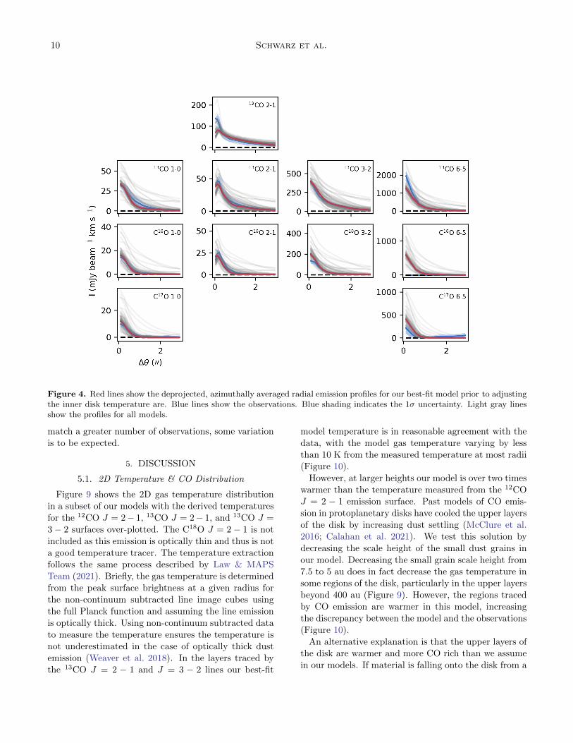
In the inner disk the model under-predicts the
strength of the 12CO 2-1 emission by a factor of 2.6,
while providing a reasonable fit to the emission from
the less abundant CO isotopologs (Figure 4). The emis-
sion surface profiles derived from observations show that12CO emission originates from higher in the disk than
the other lines. To fit the 12CO J = 2−1 emission in the
inner disk we increase the temperature inside of 32 au
and for Z/R > 0.1. Increasing the gas temperature by
a factor of 10 in this region, from several tens of kelvin
to several hundred kelvin, greatly improves the agree-
ment between the model 12CO J = 2 − 1 emission and
the observations without significantly increasing emis-
sion from the other lines (Figure 5). Possible sources
of this extra heating are discussed below. Increasing
the temperature in the inner disk has a negligible effect
on the model HD flux. This model, with an increased
temperature in the inner disk, provides the best fit to
the data. The input values for our best-fit model are
shown in Table 6 and the 2D hydrogen gas distribution,
dust temperature, and gas temperature are shown in
Figure 6. However, because of our sparsely sampled pa-
rameter space we cannot rule out the possibility of other
model solutions fitting the data equally well.
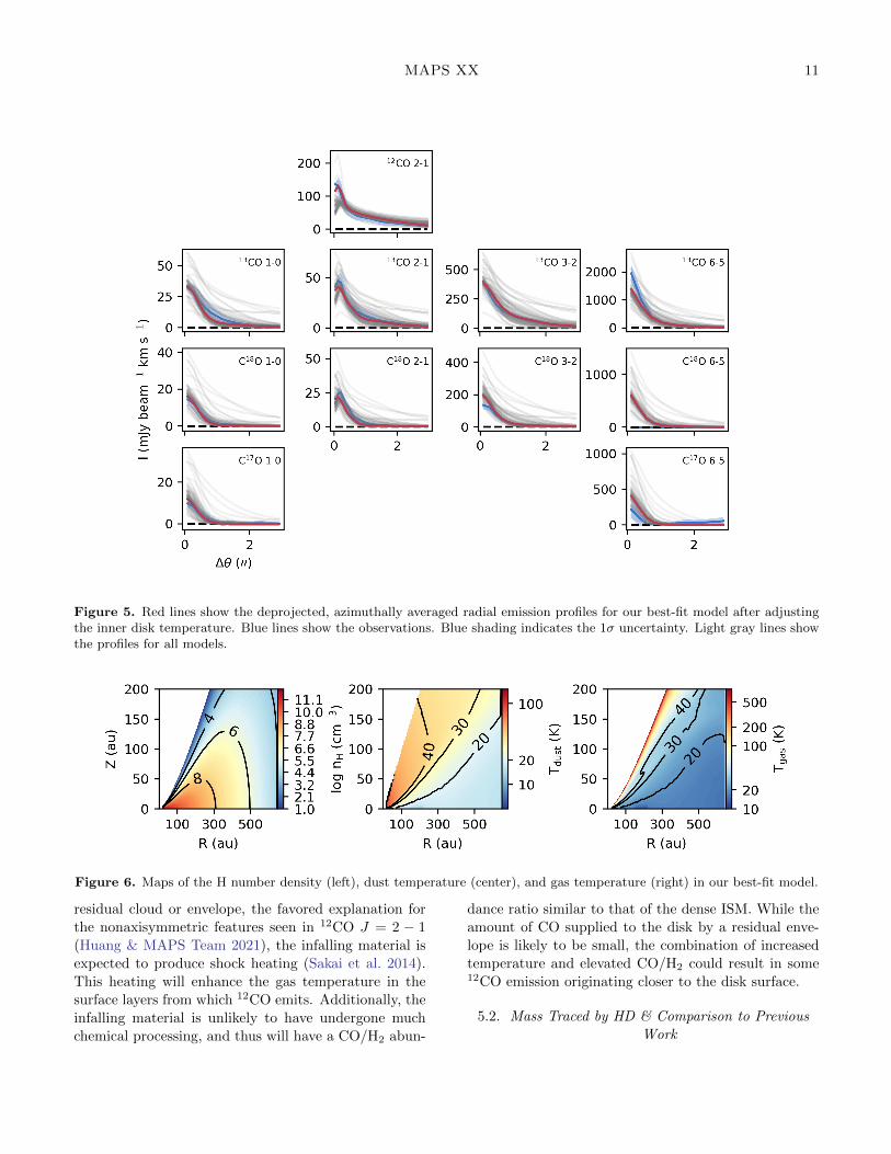
In order to match the 12CO 2-1 flux in the inner disk,
we need to increase the gas temperature in the surface
layers of the inner disk. The primary source of dust

8 Schwarz et al.
Figure 2. Red lines show the deprojected, azimuthally averaged radial emission profiles for our model using the same diskdensity parameters as Zhang & MAPS Team (2021). Blue lines show the observations. Blue shading indicates the 1σ uncertainty.Light gray lines show the profiles for all models.
Table 6. Gas and Dust Population Parameters:best-fit model Values
Gas Small Dust Large Dust
Mass (M) 0.2 1.03 × 10⁻⁴ 5.94 × 10⁻⁴
ψ 1.5 1.5 2.0
γ 0.59 0.59 1.0
Rc (au) 111 111 · · ·Rref (au) 100 100 100
href (au) 7.5 7.5 1.0
Rin (au) 15 1.0 0.45
Rout (au) 650 650 600
heating in RAC2D is radiation from the central star. The
gas temperature is initially assumed to be the same as
the dust temperature and allowed to evolve due to a
number of heating and cooling processes, including pho-
toelectric heating, endothermic and exothermic chemical
reactions, and viscous dissipation (Du & Bergin 2014).
However, in the surface layers of the inner disk pho-
toelectric heating of polycyclic aromatic hydrocarbons
(PAHs) can be an important contributor to the local gas
temperature (Kamp & Dullemond 2004; Woitke et al.2016). While heating by PAHs is included in RAC2D, the
PAH abundance in the disk surface layers is uncertain.
We assume a PAH abundance relative to H of 1.6× 10⁻⁷
(Du & Bergin 2014). A higher PAH abundance could
result in increased photoelectric heating and thus in a
warmer disk surface.
Alternatively, mechanical heating mechanisms such as
stellar winds and accretion onto the central star can raise
the temperature of the inner disk. When including me-
chanical heating, both Glassgold et al. (2004) and Na-
jita & Adamkovics (2017) found temperatures of several
hundred kelvin for vertical column densities equivalent
to those in the region of our model where we artificially
increase the temperature, though these models looked
at full disks without a large central dust cavity as seen
in the GM Aur disk. Calahan & MAPS Team (2021)
also found that their RAC2D model requires additional

MAPS XX 9
Figure 3. Extracted emission surface profiles for the 12CO 2-1, 13CO 3-2, 13CO 2-1, and C18O 2-1 lines in our observations(blue) and three models (red). Shading indicates the uncertainty based on the scatter of points in the extraction before averaging.From left to right the columns show our results for the model using the disk parameters from Zhang & MAPS Team (2021),our best-fit model, and our best-fit model with small grain setteling.
heating to match the observed 12CO J = 2 − 1 flux in
the HD 163296 disk inside of 32 au, further suggesting
that under-predicting emission in the surface layers of
the inner disk is due to limitations in the code.
4.1. CO Abundance
Figure 7 shows the CO abundance relative to H2 as
a function of height and radius in our best-fit model.
CO is effectively frozen out from the gas near the mid-
plane from 75 to 250 au. Outside the millimeter dust
disk, the gas temperature remains below the CO freeze-
out temperature. However, nonthermal desorption by
UV photons allows some CO to remain in the gas (e.g.,
Oberg et al. 2015). In the region directly above the
CO freeze-out layer, gas-phase CO has been converted
into CO2 ice (e.g., Reboussin et al. 2015; Bosman et al.
2018). Closer to the disk surface, where the temperature
exceeds the CO2 freeze-out temperature, CO remains in
the gas.
Figure 8 compares the CO depletion profile after
evolving the chemistry in our best-fit model for 1 Myr
to that found by Zhang & MAPS Team (2021). Both re-
sults follow the general trend of a roughly constant, highlevel of CO depletion outside of roughly 100 au, with the
inner disk less depleted in CO. The location of the mid-
plane CO snowline in our model, here defined as where
the CO gas and ice abundances are equal, is 31 au, con-
sistent with the derived CO snowline of 30± 5 au from
Zhang & MAPS Team (2021). Our model has greater
CO depletion inside 200 au, as well as a more abrupt
return of CO in the inner disk compared to the Zhang
& MAPS Team (2021) results. The abrupt change in
the CO column is due to the conversion of CO gas into
CO2 ice and CH4 ice near the midplane from roughly
90-150 au, which is not seen to the same extent in the
Zhang & MAPS Team (2021) model. Given that the two
approaches remove CO from the disk at different points
in the modeling process, and that this work attempts to
10 Schwarz et al.
Figure 4. Red lines show the deprojected, azimuthally averaged radial emission profiles for our best-fit model prior to adjustingthe inner disk temperature are. Blue lines show the observations. Blue shading indicates the 1σ uncertainty. Light gray linesshow the profiles for all models.
match a greater number of observations, some variation
is to be expected.
5. DISCUSSION
5.1. 2D Temperature & CO Distribution
Figure 9 shows the 2D gas temperature distribution
in a subset of our models with the derived temperatures
for the 12CO J = 2− 1, 13CO J = 2− 1, and 13CO J =
3− 2 surfaces over-plotted. The C18O J = 2− 1 is not
included as this emission is optically thin and thus is not
a good temperature tracer. The temperature extraction
follows the same process described by Law & MAPS
Team (2021). Briefly, the gas temperature is determined
from the peak surface brightness at a given radius for
the non-continuum subtracted line image cubes using
the full Planck function and assuming the line emission
is optically thick. Using non-continuum subtracted data
to measure the temperature ensures the temperature is
not underestimated in the case of optically thick dust
emission (Weaver et al. 2018). In the layers traced by
the 13CO J = 2 − 1 and J = 3 − 2 lines our best-fit
model temperature is in reasonable agreement with the
data, with the model gas temperature varying by less
than 10 K from the measured temperature at most radii
(Figure 10).
However, at larger heights our model is over two times
warmer than the temperature measured from the 12CO
J = 2 − 1 emission surface. Past models of CO emis-
sion in protoplanetary disks have cooled the upper layers
of the disk by increasing dust settling (McClure et al.
2016; Calahan et al. 2021). We test this solution by
decreasing the scale height of the small dust grains in
our model. Decreasing the small grain scale height from
7.5 to 5 au does in fact decrease the gas temperature in
some regions of the disk, particularly in the upper layers
beyond 400 au (Figure 9). However, the regions traced
by CO emission are warmer in this model, increasing
the discrepancy between the model and the observations
(Figure 10).
An alternative explanation is that the upper layers of
the disk are warmer and more CO rich than we assume
in our models. If material is falling onto the disk from a
MAPS XX 11
Figure 5. Red lines show the deprojected, azimuthally averaged radial emission profiles for our best-fit model after adjustingthe inner disk temperature. Blue lines show the observations. Blue shading indicates the 1σ uncertainty. Light gray lines showthe profiles for all models.
Figure 6. Maps of the H number density (left), dust temperature (center), and gas temperature (right) in our best-fit model.
residual cloud or envelope, the favored explanation for
the nonaxisymmetric features seen in 12CO J = 2 − 1
(Huang & MAPS Team 2021), the infalling material is
expected to produce shock heating (Sakai et al. 2014).
This heating will enhance the gas temperature in the
surface layers from which 12CO emits. Additionally, the
infalling material is unlikely to have undergone much
chemical processing, and thus will have a CO/H2 abun-
dance ratio similar to that of the dense ISM. While the
amount of CO supplied to the disk by a residual enve-
lope is likely to be small, the combination of increased
temperature and elevated CO/H2 could result in some12CO emission originating closer to the disk surface.
5.2. Mass Traced by HD & Comparison to Previous
Work

12 Schwarz et al.
Figure 7. Map of CO abundance relative to H2 in our best-fit model.
Figure 11 shows the distribution of the HD emission
in our best-fit model. Seventy-five percent of the HD
emission originates from the inner 100 au. In particular,
the hot, low density gas inside the millimeter dust inner
radius at 32 au contributes a non-negligible amount to
the HD flux. In comparison, only 47% of the total disk
gas mass is inside 100 au. Since HD does not readily
emit at temperatures less than ∼ 20 K, much of the disk
beyond 100 au is not well traced by the HD J = 1 − 0
emission. There may be more mass in the outer disk
than accounted for in our best-fit model. Additional
analysis, e.g., using CS emission (Teague et al. 2018), is
needed to better constrain the gas density in the outer
disk.
Previous analysis of the HD detection by McClure
et al. (2016) in GM Aur constrains the disk gas mass
to 0.025-0.204 M. Based on analysis of the millimeter
and centimeter continuum, Macıas et al. (2018) found a
total dust mass of 2 MJ. Assuming a gas-to-dust mass
ratio of 100, this corresponds to a total gas mass of 0.19M, at the high end of the range given by McClure et al.
(2016). Trapman et al. (2017) reanalyzed the HD detec-
tion in GM Aur by comparing to the HD line flux in a
grid of generic 2D thermochemical models. They con-
strained the mass of the GM Aur disk to be between
0.01 M and a few tenths of a solar mass. Woitke et al.
(2019) have also built a model of the GM Aur disk as
part of the DIANA project. Their model based on the
observed SED has a total disk mass of 0.11 M and also
reasonably reproduces the observed total flux of the 63
µm [OI] line as well as the 12CO 2-1 and HCO+ 3-2
lines. Their final model, independent of the SED fit
and based on Submillimeter Array (SMA) observations
of the 12CO J = 2-1 line, has a disk mass of 3.3× 10⁻²
M.
Our best-fit model has a total gas mass of 0.2 M,
consistent with the upper limits of previous works. This
Figure 8. Top: CO column density profile for our best-fitmodel and for the best-fit model of Zhang & MAPS Team(2021). Bottom: CO depletion factor as a function of radiusfor our best-fit model after evolving the chemistry for 1 Myr,as well as the best-fit model of Zhang & MAPS Team (2021)relative to the initial CO abundance. Vertical gray line inthe midplane CO snowline at 31 au in our model. Horizontaldashed lines indicate depletion factors of 10 and 100.
high value comes in part from our overall low disk tem-
perature, needed to match the gas temperature from CO
observations. Additionally, previous works have set the
outer radius of the disk to 250-300 au. Here we set the
disk outer radius to 650 au based on the observed ex-
tent of the 12CO 2-1 emission, though less than 3% of
the total gas mass is outside of 300 au.
5.3. Disk Stability
The stability of a rotating disk against gravitational
collapse is often characterized using the Toomre Q pa-

MAPS XX 13
Figure 9. Temperatures of the emission surfaces derived from 12CO, and 13CO 2-1 the 13CO 3-2 observations overlaid on thegas temperature map from our best-fit model.
Figure 10. Temperatures of the emission surfaces derived from 12CO 2-1, 13CO 2-1, and 13CO 3-2 observations (blue) comparedto the temperature of the corresponding location in our models (red).
rameter (Toomre 1964):
Q =csΩ
πGΣ(4)
where cs is the gas sound speed assuming the midplane
gas temperature, Ω is the Keplerian angular velocity of
the disk, and Σ is the total gas+dust surface density.
For a geometrically thin disk Q ∼ 1 is needed for den-
sity perturbations to develop. However, numerical sim-
ulations demonstrate that instabilities can develop for
Q < 1.7 in systems not well approximated by a geomet-
rically thin disk (Helled et al. 2014). Figure 12 shows
the Toomre Q radial profile using values from our best
fit disk model.
Our calculated Q value for GM Aur is greater than
1.7 throughout much of the disk. In the outer disk,
where spiral-like features are seen in the 12CO 2-1 emis-
sion, our calculated Q is extremely high, ranging from
∼ 7 at 250 au to ∼ 700 at 500 au. The two values in
our model that determine Q are temperature and sur-
face density. Without changing the surface density, themidplane temperature at 250 au would need to be un-
realistically low, ∼ 1 K, to reach a Q of 1.7.
As discussed in the previous section, the HD detec-
tion does not constrain the gas surface density in the
outer disk. The model surface density would need to
be increased by a factor of four at 250 au to reach Q
of 1.7 while holding the temperature constant. Zhang
& MAPS Team (2021) note that for four out of the five
MAPS sources, including GM Aur, the CO column den-
sity profiles are very shallow, consistent with a viscously
evolving disk. This supports the conclusion of Huang &
MAPS Team (2021), who argue against the nonaxisym-
metric features seen in 12CO J = 2 − 1 being driven
exclusively by disk instability based on the kinematics.
However, Q dips below 1.7 from 70 to 100 au, corre-
sponding to the location of one of the bright rings seen in

14 Schwarz et al.
Figure 11. Top: HD J = 1− 0 emitting region in our best-fit model overlayed on a map of the gas temperature. Thegray contour contains the middle 75% of the HD emission.Middle: Deprojected, azimuthally averaged radial profile forthe HD J = 1− 0 emission. Since the observed HD emissionis spatially unresolved, the model is not convolved with abeam. Bottom: Plot showing the total HD flux (blue) andgas mass (red) interior to a given radius. The HD emissionpreferentially originates from the warm inner disk.
the continuum. The concentration of large dust grains in
this region increases the disk opacity and thus decreases
the temperature of both the gas and the dust. This lower
temperature, in turn, results in a lower sound speed and
thus in a lower Toomre Q value. The presence of dust
rings and gaps can lower the midplane temperature in
a dust ring by several kelvin compared to a disk with a
smoothly varying surface density profile (Facchini et al.
2018; van der Marel et al. 2018; Alarcon et al. 2020;
Calahan & MAPS Team 2021).
The dip in the Toomre Q in our model is due en-
tirely to an over-density of dust. Our model is able to
fit the CO emission profiles in this region without a cor-
responding increase in the gas density. Decreasing the
disk surface density to 88% of our assumed value be-
tween 70 and 100 au would bring the dust ring into a
gravitationally stable regime. Alternatively, a warmer
temperature than assumed would also lead to a higher
Q. Between 70 and 100 au our model midplane tem-
perature is ∼ 12 K. The temperature derived from the
observed 13CO 2-1 line is ∼ 22 K and can be considered
an upper limit on the midplane temperature. We use
the temperature from 13CO because the C18O is opti-
cally thin at these radii and therefore not a good tracer
of temperature. Taking the midplane temperature to be
22 K increases the Q value to 2.0. Interestingly, recent
smoothed particle hydrodynamics modeling shows that
a migrating planet can increase the local disk temper-
ature, suppressing spiral structure and stabilizing the
disk (Rowther et al. 2020).
GI is thought to primarily manifest as nonaxisymmet-
ric features. Previous analysis of the continuum disk
emission at FUV wavelengths does not indicate any
such features in the 70-120 au range (Hornbeck et al.
2016). No nonaxisymmetric substructure is seen in the
CO emission profiles in this region. However, the in-
tensity of the bright continuum ring at 40 au at 7 mm
shows a low signal-to-noise (∼ 2σ) asymmetry (Macıas
et al. 2018). While the ring at 84 au is not detected at
7 mm with high enough sensitivity to enable a similar
analysis, Huang et al. (2020) note that the 84 au ring
is nonaxisymmetric at 1.1 mm. The ring appears wider
along the major axis of the disk, which as Huang et al.
(2020) demonstrate is unlikely to be an imaging arti-
fact; instead the variation can be attributed to either
nonaxisymmetric or vertical structure within the ring.
An interesting point of comparison is the HL Tau disk,
which, though less evolved than GM Aur, has a similar
total gas mass and a region of instability centered on a
dust gap (Booth & Ilee 2020). Spiral structure is also
seen in the HCO+ J = 3-2 emission toward HL Tau (Yen
et al. 2019). While this spiral structure was originally
attributed to the infalling envelope, Booth & Ilee (2020)
note that the feature could also be associated with the
region of instability in the disk. Conversely, observa-
tions of HCO+ J = 3-2 toward GM Aur do not appear
to deviate substantially from Keplerian rotation (Huang

MAPS XX 15
Figure 12. Top: Calculated Toomre Q value. Dotted lineindicates the gravitationally unstable threshold of 1.7 for ageometrically thick disk. Bottom: Midplane temperatureas a function of radius in our best-fit model. Dashed line isthe gas temperature derived from the 13CO 2-1 observations.gray regions indicate the locations of the observed gaps inthe millimeter continuum (Macıas et al. 2018). The dips intemperature, and, by extension, Q, corresponds to brightrings in the continuum.
et al. 2020). It is possible that the GM Aur disk is in the
process of stabilizing after a period of infall or planet
formation. Given the limitations of using Toomre Q
to determine the stability of the non-geometrically thin
disk, a more detailed study of the kinematics is required
to determine the stability of the GM Aur disk from 70
to 100 au.
6. SUMMARY AND CONCLUSIONS
In this work we use observations of CO isotopologs in
the GM Aur disk taken as part of the MAPS ALMA
Large Program along with archival observations of CO
from ALMA and HD from Herschel to build a model of
the disk gas density and temperature structure. Based
on our results we conclude the following:
• Much of the disk (32% by mass) is cooler than
20 K. As such the HD emission only traces the
inner 200 au, while the gas disk extends to 650 au
based on observations of 12CO.
• We constrain the gas mass of the GM Aur disk to
be ∼ 0.2 M. While the total mass in the outer
disk remains somewhat uncertain, only 15% of the
mass in our best-fit model is beyond 200 au. Any
variation in mass in the outer disk will likely have
only a small aefect on the total disk mass.
• The CO gas abundance relative to H2 is reduced
by approximately one order of magnitude with re-
spect to the ISM values inside 100 au and by two
orders of magnitude outside 100 au. This is con-
sistent with the analysis of Zhang & MAPS Team
(2021). Our model also shows CO gas returning
to the midplane outside of the millimeter dust disk
due to nonthermal desorption.
• Based on the calculated Toomre Q parameter, the
outer disk appears stable against gravitational col-
lapse. However, Q dips into the unstable regime
between 70 and 100 au, corresponding to the sec-
ond bright ring seen in millimeter dust emission.
While there is some evidence for nonaxisymmetric
features in the dust continuum at these radii, a
more detailed study is needed to determine if the
GM Aur disk is gravitationally unstable.
ACKNOWLEDGMENTS
This paper makes use of the following ALMA
data: ADS/JAO.ALMA#2016.1.00565.S and
ADS/JAO.ALMA#2018.1.01055.L. ALMA is a part-
nership of ESO (representing its member states),
NSF (USA) and NINS (Japan), together with NRC
(Canada), MOST and ASIAA (Taiwan), and KASI
(Republic of Korea), in cooperation with the Republic
of Chile. The Joint ALMA Observatory is operated
by ESO, AUI/NRAO and NAOJ. The National Radio
Astronomy Observatory is a facility of the National Sci-
ence Foundation operated under cooperative agreement
by Associated Universities, Inc. This work is based on
observations made with Herschel, a European Space
Agency Cornerstone Mission with significant participa-
tion by NASA.

16 Schwarz et al.
K.R.S., K.Z., J.B., J.H., and I.C. acknowledge the
support of NASA through Hubble Fellowship Program
grants HST-HF2-51419.001, HST-HF2-51401.001, HST-
HF2-51427.001-A, HST-HF2-51460.001-A, and HST-
HF2-51405.001-A awarded by the Space Telescope Sci-
ence Institute, which is operated by the Associa-
tion of Universities for Research in Astronomy, Inc.,
for NASA, under contract NAS5-26555. J.K.C. ac-
knowledges support from the National Aeronautics and
Space Administration FINESST grant, under Grant no.
80NSSC19K1534. C.J.L. and J.K.C. acknowledge fund-
ing from the National Science Foundation Graduate Re-
search Fellowship under Grant No. DGE1745303 and
DGE1256260. K.Z. acknowledges the support of the
Office of the Vice Chancellor for Research and Grad-
uate Education at the University of Wisconsin – Madi-
son with funding from the Wisconsin Alumni Research
Foundation. Y.A. acknowledges support by NAOJ
ALMA Scientific Research Grant Code 2019-13B, and
Grant-in-Aid for Scientific Research Nos. 18H05222
and 20H05847. S.A. and J.H. acknowledge funding sup-
port from the National Aeronautics and Space Admin-
istration under Grant No. 17-XRP17 2-0012 issued
through the Exoplanets Research Program. E.A.B.,
A.D.B., and F.A. acknowledge support from NSF AAG
Grant #1907653. A.S.B. acknowledges the studentship
funded by the Science and Technology Facilities Council
of the United Kingdom (STFC). G.C. is supported by
NAOJ ALMA Scientific Research grant Code 2019-13B.
L.I.C. gratefully acknowledges support from the David
and Lucille Packard Foundation and Johnson & John-
son’s WiSTEM2D Program. J.D.I. acknowledges sup-
port from the Science and Technology Facilities Council
of the United Kingdom (STFC) under ST/T000287/1.
R.L.G. acknowledges support from a CNES research fel-
lowship. F.L. and R.T. acknowledge support from the
Smithsonian Institution as Submillimeter Array (SMA)
Fellows. Y.L. acknowledges the financial support by
the Natural Science Foundation of China (Grant No.
11973090). F.M. acknowledges support from ANR
of France under contract ANR-16-CE31-0013 (Planet-
Forming-Disks) and ANR-15-IDEX-02 (through CDP
“Origins of Life”). K.I.O. acknowledges support from
the Simons Foundation (SCOL #321183) and an NSF
AAG Grant (#1907653). C.W. acknowledges finan-
cial support from the University of Leeds, STFC and
UKRI (grant numbers ST/R000549/1, ST/T000287/1,
MR/T040726/1).
Facilities: ALMA, Herschel
Software: analysisUtils (https://casaguides.
nrao.edu/index.php/Analysis Utilities), astropy (As-
tropy Collaboration et al. 2013), CASA (McMullin
et al. 2007), diskprojection(https://github.com/
richteague/disksurf), matplotlib (Hunter 2007), numpy
(van der Walt et al. 2011), RAC2D (Du & Bergin 2014),
RADMC-3D, (Dullemond et al. 2012), SciPy (Jones
et al. 2001–),

MAPS XX 17
REFERENCES
Alarcon, F., Teague, R., Zhang, K., Bergin, E. A., &
Barraza-Alfaro, M. 2020, ApJ, 905, 68,
doi: 10.3847/1538-4357/abc1d6
ALMA Partnership, Brogan, C. L., Perez, L. M., et al.
2015, ApJL, 808, L3, doi: 10.1088/2041-8205/808/1/L3
Andrews, S. M., Wilner, D. J., Espaillat, C., et al. 2011,
ApJ, 732, 42, doi: 10.1088/0004-637X/732/1/42
Ansdell, M., Williams, J. P., van der Marel, N., et al. 2016,
ApJ, 828, 46, doi: 10.3847/0004-637X/828/1/46
Astropy Collaboration, Robitaille, T. P., Tollerud, E. J.,
et al. 2013, A&A, 558, A33,
doi: 10.1051/0004-6361/201322068
Bergin, E. A., & Williams, J. P. 2017, The Determination
of Protoplanetary Disk Masses, ed. M. Pessah &
O. Gressel, Vol. 445, 1, doi: 10.1007/978-3-319-60609-5 1
Bergin, E. A., Cleeves, L. I., Gorti, U., et al. 2013, Nature,
493, 644, doi: 10.1038/nature11805
Birnstiel, T., Dullemond, C. P., Zhu, Z., et al. 2018, ApJL,
869, L45, doi: 10.3847/2041-8213/aaf743
Booth, A. S., & Ilee, J. D. 2020, MNRAS, 493, L108,
doi: 10.1093/mnrasl/slaa014
Booth, A. S., Walsh, C., Ilee, J. D., et al. 2019, ApJL, 882,
L31, doi: 10.3847/2041-8213/ab3645
Bosman, A. D., Walsh, C., & van Dishoeck, E. F. 2018,
A&A, 618, A182, doi: 10.1051/0004-6361/201833497
Boss, A. P. 1997, Science, 276, 1836,
doi: 10.1126/science.276.5320.1836
Calahan, J., & MAPS Team. 2021, ApJ, 0, 0, doi: 0
Calahan, J. K., Bergin, E., Zhang, K., et al. 2021, ApJ,
908, 8, doi: 10.3847/1538-4357/abd255
Calvet, N., D’Alessio, P., Watson, D. M., et al. 2005, ApJL,
630, L185, doi: 10.1086/491652
Cleeves, L. I., Adams, F. C., & Bergin, E. A. 2013, ApJ,
772, 5, doi: 10.1088/0004-637X/772/1/5
Czekala, I., & MAPS Team, A. 2021, ApJ, 0, 0, doi: 0
Du, F., & Bergin, E. A. 2014, ApJ, 792, 2,
doi: 10.1088/0004-637X/792/1/2
Dullemond, C. P., Juhasz, A., Pohl, A., et al. 2012,
RADMC-3D: A multi-purpose radiative transfer tool.
http://ascl.net/1202.015
Eistrup, C., Walsh, C., & van Dishoeck, E. F. 2018, A&A,
613, A14, doi: 10.1051/0004-6361/201731302
Espaillat, C., Furlan, E., D’Alessio, P., et al. 2011, ApJ,
728, 49, doi: 10.1088/0004-637X/728/1/49
Facchini, S., Pinilla, P., van Dishoeck, E. F., & de Juan
Ovelar, M. 2018, A&A, 612, A104,
doi: 10.1051/0004-6361/201731390
Facchini, S., van Dishoeck, E. F., Manara, C. F., et al.
2019, A&A, 626, L2, doi: 10.1051/0004-6361/201935496
Favre, C., Cleeves, L. I., Bergin, E. A., Qi, C., & Blake,
G. A. 2013, ApJL, 776, L38,
doi: 10.1088/2041-8205/776/2/L38
Gaia Collaboration, Brown, A. G. A., Vallenari, A., et al.
2018, A&A, 616, A1, doi: 10.1051/0004-6361/201833051
Glassgold, A. E., Najita, J., & Igea, J. 2004, ApJ, 615, 972,
doi: 10.1086/424509
Guilloteau, S., & Dutrey, A. 1998, A&A, 339, 467
Hasegawa, T. I., Herbst, E., & Leung, C. M. 1992, ApJS,
82, 167, doi: 10.1086/191713
Helled, R., Bodenheimer, P., Podolak, M., et al. 2014, in
Protostars and Planets VI, ed. H. Beuther, R. S. Klessen,
C. P. Dullemond, & T. Henning, 643,
doi: 10.2458/azu uapress 9780816531240-ch028
Hogerheijde, M. R., Bergin, E. A., Brinch, C., et al. 2011,
Science, 334, 338, doi: 10.1126/science.1208931
Hornbeck, J. B., Swearingen, J. R., Grady, C. A., et al.
2016, ApJ, 829, 65, doi: 10.3847/0004-637X/829/2/65
Huang, J., & MAPS Team. 2021, ApJ, 0, 0, doi: 0
Huang, J., Andrews, S. M., Dullemond, C. P., et al. 2020,
ApJ, 891, 48, doi: 10.3847/1538-4357/ab711e
Hughes, A. M., Andrews, S. M., Espaillat, C., et al. 2009,
ApJ, 698, 131, doi: 10.1088/0004-637X/698/1/131
Hunter, J. D. 2007, Computing in Science and Engineering,
9, 90, doi: 10.1109/MCSE.2007.55
Isella, A., Guidi, G., Testi, L., et al. 2016, PhRvL, 117,
251101, doi: 10.1103/PhysRevLett.117.251101
Jones, E., Oliphant, T., Peterson, P., et al. 2001–, SciPy:
Open source scientific tools for Python.
http://www.scipy.org/
Kama, M., Trapman, L., Fedele, D., et al. 2020, A&A, 634,
A88, doi: 10.1051/0004-6361/201937124
Kamp, I., & Dullemond, C. P. 2004, ApJ, 615, 991,
doi: 10.1086/424703
Krijt, S., Schwarz, K. R., Bergin, E. A., & Ciesla, F. J.
2018, ApJ, 864, 78, doi: 10.3847/1538-4357/aad69b
Law, C., & MAPS Team. 2021, ApJ, 0, 0, doi: 0
Linsky, J. L. 1998, SSRv, 84, 285
Liu, S.-F., Jin, S., Li, S., Isella, A., & Li, H. 2018, ApJ,
857, 87, doi: 10.3847/1538-4357/aab718
Long, F., Herczeg, G. J., Pascucci, I., et al. 2017, ApJ, 844,
99, doi: 10.3847/1538-4357/aa78fc
Lynden-Bell, D., & Pringle, J. E. 1974, MNRAS, 168, 603,
doi: 10.1093/mnras/168.3.603
Macıas, E., Espaillat, C. C., Ribas, A., et al. 2018, ApJ,
865, 37, doi: 10.3847/1538-4357/aad811
Mathis, J. S., Rumpl, W., & Nordsieck, K. H. 1977, ApJ,
217, 425, doi: 10.1086/155591

18 Schwarz et al.
McClure, M. K., Bergin, E. A., Cleeves, L. I., et al. 2016,
ApJ, 831, 167, doi: 10.3847/0004-637X/831/2/167
McMullin, J. P., Waters, B., Schiebel, D., Young, W., &
Golap, K. 2007, in Astronomical Society of the Pacific
Conference Series, Vol. 376, Astronomical Data Analysis
Software and Systems XVI, ed. R. A. Shaw, F. Hill, &
D. J. Bell, 127
Miotello, A., Bruderer, S., & van Dishoeck, E. F. 2014,
A&A, 572, A96, doi: 10.1051/0004-6361/201424712
Najita, J. R., & Adamkovics, M. 2017, ApJ, 847, 6,
doi: 10.3847/1538-4357/aa8632
Najita, J. R., & Bergin, E. A. 2018, ApJ, 864, 168,
doi: 10.3847/1538-4357/aad80c
Oberg, K. I., Furuya, K., Loomis, R., et al. 2015, ApJ, 810,
112, doi: 10.1088/0004-637X/810/2/112
Oberg, K. I., & MAPS Team. 2021, ApJ, 0, 0, doi: 0
Pinte, C., Price, D. J., Menard, F., et al. 2018, ApJ, 860,
L13, doi: 10.3847/2041-8213/aac6dc
Powell, D., Murray-Clay, R., Perez, L. M., Schlichting,
H. E., & Rosenthal, M. 2019, ApJ, 878, 116,
doi: 10.3847/1538-4357/ab20ce
Powell, D., Murray-Clay, R., & Schlichting, H. E. 2017,
ApJ, 840, 93, doi: 10.3847/1538-4357/aa6d7c
Reboussin, L., Wakelam, V., Guilloteau, S., Hersant, F., &
Dutrey, A. 2015, A&A, 579, A82,
doi: 10.1051/0004-6361/201525885
Rowther, S., Meru, F., Kennedy, G. M., Nealon, R., &
Pinte, C. 2020, ApJL, 904, L18,
doi: 10.3847/2041-8213/abc704
Sakai, N., Oya, Y., Sakai, T., et al. 2014, ApJL, 791, L38,
doi: 10.1088/2041-8205/791/2/L38
Schwarz, K. R., Bergin, E. A., Cleeves, L. I., et al. 2016,
ApJ, 823, 91, doi: 10.3847/0004-637X/823/2/91
—. 2018, ApJ, 856, 85, doi: 10.3847/1538-4357/aaae08
Teague, R., Bae, J., Bergin, E. A., Birnstiel, T., &
Foreman-Mackey, D. 2018, ApJ, 860, L12,
doi: 10.3847/2041-8213/aac6d7
Tobin, J. J., Looney, L. W., Li, Z.-Y., et al. 2018, ApJ, 867,
43, doi: 10.3847/1538-4357/aae1f7
Toomre, A. 1964, ApJ, 139, 1217, doi: 10.1086/147861
Trapman, L., Facchini, S., Hogerheijde, M. R., van
Dishoeck, E. F., & Bruderer, S. 2019, A&A, 629, A79,
doi: 10.1051/0004-6361/201834723
Trapman, L., Miotello, A., Kama, M., van Dishoeck, E. F.,
& Bruderer, S. 2017, A&A, 605, A69,
doi: 10.1051/0004-6361/201630308
van der Marel, N., Williams, J. P., Ansdell, M., et al. 2018,
ApJ, 854, 177, doi: 10.3847/1538-4357/aaaa6b
van der Walt, S., Colbert, S. C., & Varoquaux, G. 2011,
Computing in Science and Engineering, 13, 22,
doi: 10.1109/MCSE.2011.37
Weaver, E., Isella, A., & Boehler, Y. 2018, ApJ, 853, 113,
doi: 10.3847/1538-4357/aaa481
Williams, J. P., & Best, W. M. J. 2014, ApJ, 788, 59,
doi: 10.1088/0004-637X/788/1/59
Wilson, T. L. 1999, Reports on Progress in Physics, 62,
143, doi: 10.1088/0034-4885/62/2/002
Woitke, P., Min, M., Pinte, C., et al. 2016, A&A, 586,
A103, doi: 10.1051/0004-6361/201526538
Woitke, P., Kamp, I., Antonellini, S., et al. 2019, PASP,
131, 064301, doi: 10.1088/1538-3873/aaf4e5
Woodall, J., Agundez, M., Markwick-Kemper, A. J., &
Millar, T. J. 2007, A&A, 466, 1197,
doi: 10.1051/0004-6361:20064981
Xu, R., Bai, X.-N., & Oberg, K. 2017, ApJ, 835, 162,
doi: 10.3847/1538-4357/835/2/162
Yen, H.-W., Gu, P.-G., Hirano, N., et al. 2019, ApJ, 880,
69, doi: 10.3847/1538-4357/ab29f8
Yu, M., Willacy, K., Dodson-Robinson, S. E., Turner, N. J.,
& Evans, II, N. J. 2016, ApJ, 822, 53,
doi: 10.3847/0004-637X/822/1/53
Zhang, & MAPS Team. 2021, ApJ, 0, 0, doi: 0
Zhang, K., Bergin, E. A., Blake, G. A., Cleeves, L. I., &
Schwarz, K. R. 2017, Nature Astronomy, 1, 0130,
doi: 10.1038/s41550-017-0130


